Fusion of CMONOC and ERA5 PWV Products Based on Backpropagation Neural Network

Abstract

Data fusion is an effective method to obtain high-precision and high-spatiotemporal-resolution precipitable water vapor (PWV) products, which play an important role in understanding climate change and meteorological monitoring. However, existing fusion methods have some shortcomings, such as ignoring the applicability of the model space or the high complexity of model operation. In this study, the high-precision and high-temporal-resolution Global Navigation Satellite System (GNSS) PWV was used to calibrate and optimize the ERA5 PWV product of the European Center for Medium-Range Weather Forecasts Reanalysis 5 (ERA5) with high spatial resolution to improve its accuracy, and its applicability was verified at the spatiotemporal scale. First, this study obtained accurate GNSS PWV from meteorological data from stations and used it as the true value to analyze the distribution of the ERA5 PWV in mainland China. The results showed that the ERA5 PWV showed significant spatial and temporal differences. Then, a backpropagation neural network (BPNN) fusion correction model with additional constraints was established. The correction results showed that the bias of the ERA5 PWV mainly fluctuated near 0, the correlation between the ERA5 PWV and GNSS PWV was increased to 0.99, and the positive improvement rate of the root-mean-square error (RMSE) was 95%. In the temporal scale validation, the RMSE of the ERA5 PWV decreased from 2.05 mm to 1.67 mm, an improvement of 18.54%. In the spatial scale validation, the RMSE of the four seasons decreased by 0.26–80% (spring), 0.28–70.71% (summer), 0.28–45.23% (autumn), and 0.30–40.75% (winter). Especially in the summer and plateau mountainous areas where the ERA5 PWV performance was poor, the model showed suitable stability. Finally, the fusion model was used to generate a new PWV product, which improved the accuracy of ERA5 PWV on the basis of ensuring the spatial resolution.

1. Introduction

Precipitable water vapor (PWV) not only plays an important role in climate change, but is also one of the main error sources of errors of satellite geodesy [1,2,3,4]. Reliable PWV information can play an important role in numerical weather prediction, catastrophic weather monitoring, and satellite geodesy corrections [5,6]. Therefore, the demand for high-precision PWV data with high spatial and temporal resolutions is increasingly urgent.

Existing methods for obtaining PWV data include radiosonde, satellite remote sensing, global positioning system inversion, and numerical weather prediction models [7,8,9]. Sounding PWV has the highest accuracy, but its spatiotemporal resolution is low [10]. Satellite remote sensing PWV is greatly affected by weather and surface conditions, but its spatial resolution is high [11,12,13]. GNSS PWV is a popular method for obtaining high-precision PWV products that has high temporal resolution, but its spatial resolution is still limited [14,15,16]. Numerical weather forecast models can provide PWV products with uniform temporal and spatial distributions, especially the newly released ERA5 PWV with a spatial resolution of 31 km and a temporal resolution of 1 h, but it shows obvious systematic deviations in some areas, and its accuracy needs to be verified when used [17,18,19]. Therefore, differences in the spatiotemporal resolution and accuracy of a single data source may lead to different results in the same experimental analysis.

To solve the problems of spatial and temporal resolution mismatch and precision difference among PWV products, many scholars have proposed data fusion methods, i.e., integrating the advantages of multisource data to obtain high-spatiotemporal-resolution and high-precision PWV products. Popular data fusion methods use the advantages of the high precision and high temporal resolution of GNSS PWV to fuse or calibrate it with PWV products with high spatial resolution [20,21]. For example, Xiong et al. and Zhang et al. used a general regression neural network (GRNN) to fuse GNSS PWV and ERA5 PWV from mainland China and North America; the deviation between them was well calibrated, and high-precision PWV products were obtained [22,23]. Liu et al. and Bai et al. used a linear fitting method to correct MODIS PWV and obtained higher-accuracy PWV products on the basis of ensuring high resolution [24,25]. In addition, Alshawaf et al. carried out related work using the kriging interpolation method to generate high-precision PWV products [26,27]. Li and Long fused MODIS PWV with ERA5 PWV in the upper reaches of Brahmaputra, and the results were in good agreement with GNSS PWV [28].

However, the above data fusion methods have some disadvantages. Fusion methods based on GRNN have high computational complexity. Limited by the quality of the source data itself, the error of MODISPWV corrected using GNSS PWV is still high. Fusion methods based on interpolation are limited by the imperfect assumption of interpolation, which leads to inevitable errors. In addition, some of the above methods lack an effective discussion of the applicability of the model at the spatial scale. Therefore, when conducting PWV data fusion, we should not only consider the difficulty of the fusion method operation but also carefully consider the idea of modeling and the selection of source data.

Considering the above problems comprehensively, GNSS PWV and ERA5 PWV with high-accuracy source data were selected for data fusion. The fusion method was a backpropagation neural network (BPNN), which was verified by Ma et al. for the Tibetan Plateau [29]. However, different from this method, the applicability of the model was discussed at temporal and spatial scales, and the differences in PWV in different periods, positions, and climate types were taken into account. The purpose of this research was to generate PWV products with more applicability, high precision, and high temporal and spatial resolution, which can not only meet the requirements for multiscale climate change analysis, but also provide services for tropospheric delay correction and numerical weather prediction. The organization of this paper is as follows: the research area, research data, and research methods are presented in Section 2. Section 3 discusses the spatiotemporal distribution of PWV in mainland China and the error distribution between ERA5 PWV and GNSS PWV. Section 4 details the PWV fusion models based on temporal and spatial scales. Section 5 generates the ERA5 correction products in mainland China. Section 6 provides the summary.

2. Research Area, Data, and Methods

2.1. Research Area

Due to the complex climate environment in mainland China and obvious geographical differences, the overall modeling workload of PWV is large, and the application of the model is inconvenient. Some research results showed that the error distribution of ERA5 PWV and GNSS PWV in China is not only related to geographical location and climate type, but also different in different seasons [30,31]. Therefore, while ensuring a sufficient modeling sample size, GNSS stations were divided into four regions according to their distribution, corresponding to the points of different colors in Figure 1.

2.2. GNSS PWV

GNSS-derived PWV can be obtained from CMONOC using the GAMIT high-precision data processing software. The processing is achieved with a GNSS observation sampling rate of 30 s, and the final ephemeris, RELAX mode, cutoff angle of 10°, and GMF mapping functions are adopted [32]. The zenith tropospheric delay (ZTD) corrections are estimated every 1 h, and the GAMIT default horizontal gradients are used. The obtained ZTD consists of the ZHD and ZWD, where the ZHD can be obtained from the following formula [21]:

$$\mathrm{ZHD}=\left(2.2779\pm 0.0024\right)\times \frac{\mathrm{Ps}}{1-0.00266\times \cos 2\mathsf{\theta }+0.00028\times \mathrm{H}},$$

(1)

where Ps is the atmospheric pressure (unit: hPa) obtained from ground weather stations collocated with GNSS stations, θ is the latitude of the GNSS station (unit: °), and H is the height of the GNSS station (unit: km).

The ZWD can be obtained from ZTD minus ZHD, and the PWV can be obtained using Equation (2).

$$\mathrm{PWV}= \mathsf{\Pi } \times \mathrm{ZWD}.$$

(2)

The conversion coefficient Π is calculated using Equation (3).

$$\mathsf{\Pi }=\frac{{10}^6}{\left[\left({\mathrm{k}}_3\times {\mathrm{T}}_{\mathrm{m}}^{-1}+{ \mathrm{k}}_2^{\prime } \right)\times { \mathrm{R}}_{\mathrm{v}}\right]},$$

(3)

where ${\mathrm{k}}_2^{\prime }$ (22.1 ± 2.2 K/hPa) and k₃ (3.735 × 10⁵ ± 0.012 × 10⁵ K²/hPa) are atmospheric refractivity constants, and R_v (4.613 × 10⁶ erg/g) is the gas constant of water vapor. Tm is the weighted mean temperature (unit: K), which is calculated using an empirical linear model derived by Bevis et al. from global radiosonde data [33].

$$\mathrm{Tm} =70.2+0.72\times \mathrm{Ts},$$

(4)

where Ts is the surface temperature (unit: K) obtained from ground weather stations collocated with GNSS stations.

To avoid introducing extra errors, the atmospheric pressure and temperature values measured by meteorological stations are used in this study. Compared with the sounding PWV, the GNSS PWV obtained by this method has an RMSE of approximately 2 mm, which meets the application requirements and can be used to evaluate and calibrate the ERA5 PWV [15,21,25]. Due to a large number of data missing from some stations, approximately 220 GNSS stations were selected for research and analysis after screening, and the obvious outliers existing in the GNSS PWV time series were deleted. The results in this paper are based on this; hence, there is no further description.

2.3. ERA5 PWV

ERA5 is the latest ECMWF reanalysis product of the fifth generation of the global atmosphere. Compared with ERA-Interim, ERA5 can provide higher-horizontal-resolution data products. Meanwhile, thanks to the development of model physics, core dynamics, and data assimilation in the past decade, it better captures the details of atmospheric phenomena and provides data with a spatial resolution of 0.25° × 0.25° and a temporal resolution of 1 h [34,35,36]. The PWV of the four grid points around the GPS station was calculated, and then the corresponding ERA5 PWV was interpolated to the corresponding GPS station using bilinear interpolation [37].

2.4. Data Matching

Since the PWV data quality of the samples affects the model performance, quality control is performed. First, the biases of the differences between the GNSS PWV and ERA5 PWV were calculated. Then, the standard deviation (STD) of the differences was calculated, and its threefold values were used as the threshold for the removal of outliers. Finally, 705,092 pairs were selected to construct the model.

2.5. Backpropagation Neural Network Model

A BPNN is an artificial neural network (ANN) with self-organizing, self-learning, and nonlinear ability [38,39,40]. The learning process of BPNN is the repeated process of information forward propagation and error backpropagation [29]. In the forward transmission process of the input signal, an initial weight is assigned to each neuron in the input layer and the hidden layer; then, the weight is transmitted to the output layer for output calculation, and compared with the expected target. If the error between the output and the target exceeds the threshold after the forward transmission, the backpropagation function is activated to adjust the function to reduce the error, and the weight and threshold are repeatedly corrected until the error value reaches the minimum. Theoretically, BPNN has the ability to approximate any complex nonlinear function [29]. Because the change in PWV is affected by many factors, in addition to being nonlinear and unstable. Therefore, this paper used the BPNN to establish a fusion model to correct ERA5 PWV. 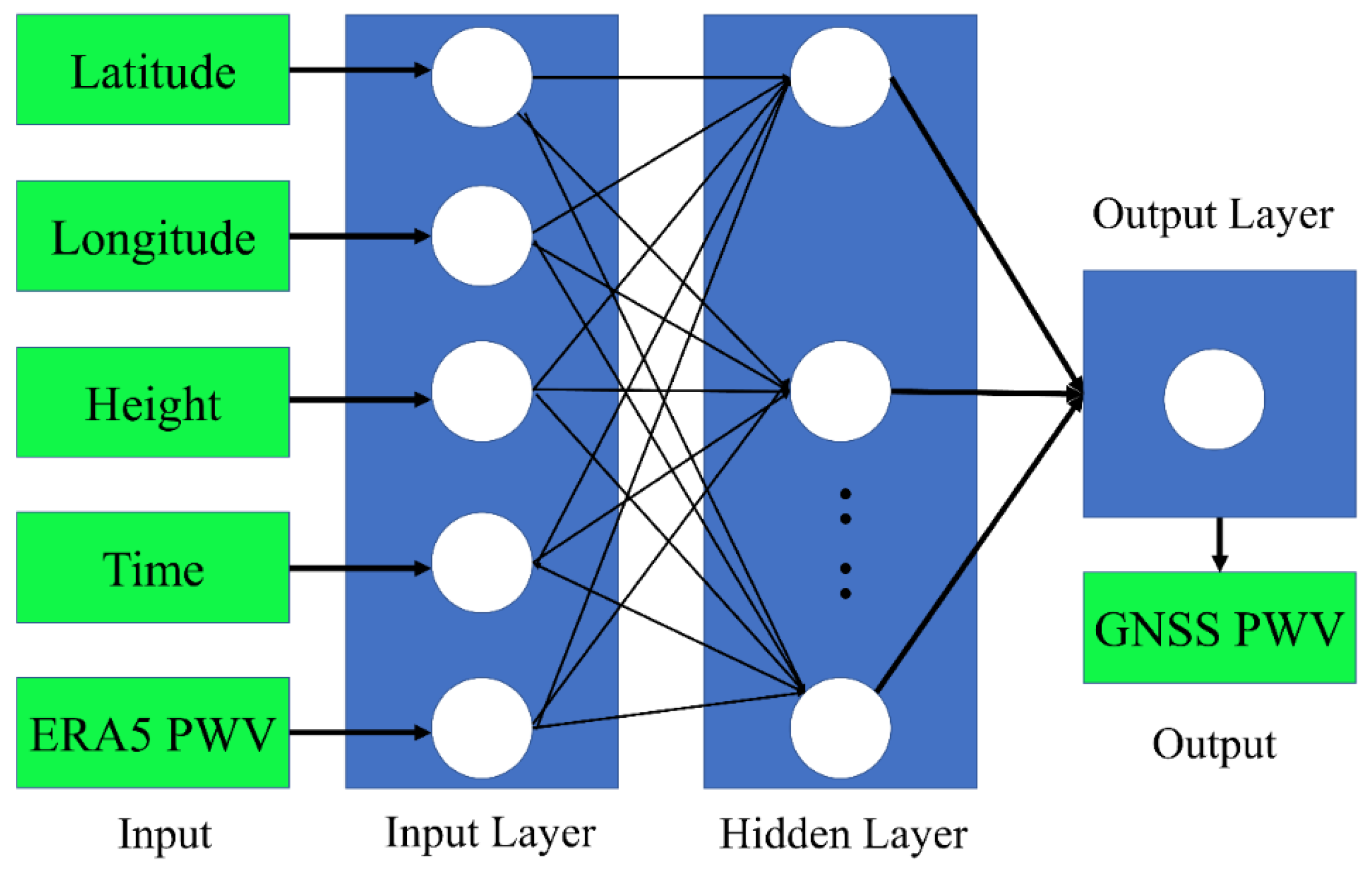Figure 2 shows the BPNN design structure adopted in this study. The input layer had five neurons corresponding to longitude, latitude, height, time, and ERA5 PWV. The output layer had only one GNSS PWV neuron.

3. PWV Distribution and ERA5 PWV Error Distribution

To discuss the temporal and spatial distribution of PWV in mainland China, this study calculated the annual average value of water vapor at GNSS stations in each climate region from 2017 to 2019. The results are shown in Figure 3a. The bias, RMSE, and correlation between the GNSS PWV and ERA5 PWV are shown in Figure 3b,c, and the overall statistics are shown in

Table 1. Bias, RMSE, and correlation between the ERA5 PWV and GNSS PWV.

Region	Average PWV (mm)	Bias (mm)	RMSE (mm)	R
SMC	28.57	0.66	2.98	0.96
TMC	16.74	−0.28	2.32	0.98
TCC	11.18	0.42	2.07	0.97
AC	10.85	1.36	2.55	0.92

Notes: bias = GNSS PWV − ERA5 PWV.

(The indicators for evaluating the difference between ERA5 PWV and GNSS PWV can be found in Appendix A).

As shown in Figure 3a, the GNSS PWV had different distribution patterns in different climatic zones in China. In the four regions, the SMC region had the highest PWV with an average value of over 28 mm, while the AC region had the lowest PWV with an average value of less than 11 mm. The average PWV values of the TMC region and TCC region were 16.74 mm and 11.18 mm, respectively. At the same latitude, the SMC region was higher than the AC region, and the TMC region was higher than the TCC region. This difference was mainly determined by the location, height, and climate type of the station. Detailed statistics are shown in Table 1.

As shown in Figure 3b and

Table 2. Bias, RMSE, and correlation between the ERA5 PWV and GNSS PWV.

Region	Season	Average PWV (mm)	Bias (mm)	RMSE (mm)	Correlation
SMC	Spring	25.49	0.45	2.55	0.96
	Summer	45.07	1.49	3.56	0.92
	Autumn	28.66	0.58	3.61	0.98
	Winter	14.01	−0.18	1.81	0.93
TMC	Spring	12.04	−0.38	1.71	0.98
	Summer	32.96	0.22	3.14	0.97
	Autumn	14.17	−0.61	2.67	0.98
	Winter	4.5	−0.36	0.87	0.94
TCC	Spring	8.59	0.23	1.65	0.96
	Summer	22.36	1.27	3.07	0.92
	Autumn	9.49	0.19	1.95	0.97
	Winter	3.48	−0.03	0.79	0.88
AC	Spring	8.72	1.23	2.12	0.92
	Summer	19.79	2.66	3.64	0.91
	Autumn	10.19	1.15	2.42	0.95
	Winter	3.93	0.32	1.23	0.80

, the ERA5 PWV values in the SMC, TCC, and AC regions were underestimated as a whole, especially in the SMC and AC regions, where individual stations could reach up to 4 mm, while, in the TMC region, it was overall overestimated, which is consistent with previous studies [7,31]. As shown in Figure 3c and Table 2, there were spatial differences in the RMSE of ERA5 PWV and GNSS PWV. The RMSE in the SMC area was highest at 2.98 mm, related to the high PWV content in the area itself, followed by the AC area, which has a complex geographical environment and high altitude, resulting in a large error of the ERA5 PWV in this area. Under the same latitude, the SMC and TMC regions had higher RMSEs. Figure 3d and Table 2 also show the correlation between the ERA5 PWV and GNSS PWV in different regions, with mean values above 0.95. The correlation between the ERA5 PWV and GNSS PWV was highest in the TMC region and lowest in the AC region. The above analysis shows that the error distribution of the ERA5 PWV was also related to its geographical location, altitude, and climate type.

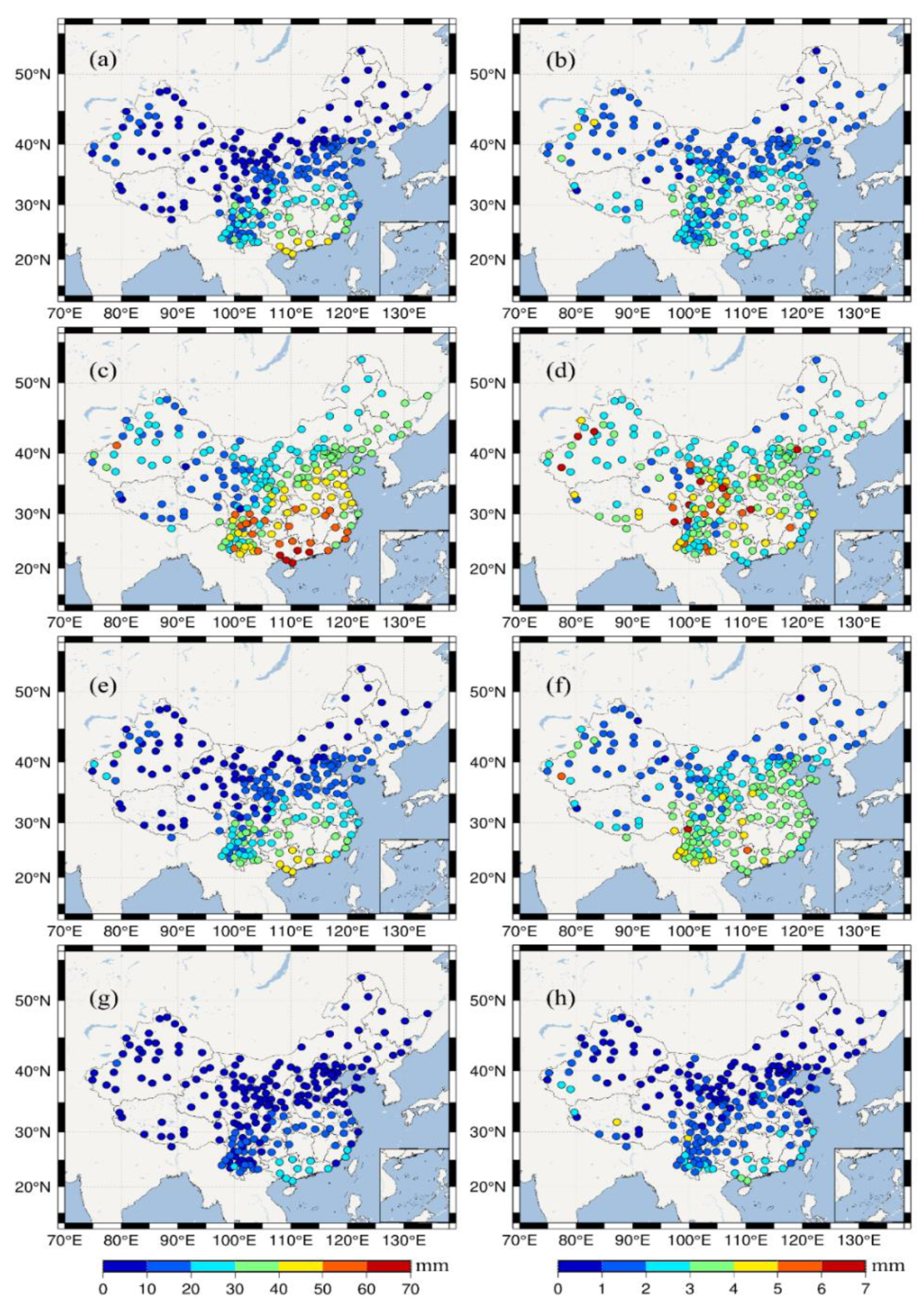
Moreover, the PWV performance in different time periods is also discussed. The PWV time series was divided into different seasons: spring (March to May), summer (June to August), autumn (September to November), and winter (December to February). Comparative analysis was also conducted in the four different climate regions, and the results are shown in Table 2. Figure 4a–h visually shows the average PWV distribution in different seasons and the RMSE of the ERA5 PWV in different seasons.

As shown in Table 2, except for the TMC region, the bias had a maximum value in summer and a minimum value in winter. The maximum value of the regional correlation appeared in autumn, and the minimum value appeared in winter. Combined with Figure 4, the PWV content was higher in summer and autumn, and the RMSE corresponding to the ERA5 PWV was larger, while it was the opposite in spring and winter. The difference in the above distribution law corresponded to the seasonal difference. The PWV content was high in summer, the precipitation was greater, and the PWV changed rapidly, resulting in a large bias and RMSE, but the opposite occurred in spring and winter, which was also the reason for the low correlation between the two in summer. The reason for the low correlation in winter was related to its PWV content, whereby even small changes would interfere with the correlation results.

The above analysis showed that the errors between the ERA5 PWV and GNSS PWV were not only affected by geographical factors, but also had different error distributions in different time periods and under different climate types. Therefore, a fusion model should be based on the temporal and spatial distributions of PWV and take the error distribution of the ERA5 PWV into account.

4. ERA5 PWV and GNSS PWV Fusion Model

To verify the applicability of the BPNN fusion model and meet the needs of different types of research, this study established two different types of fusion models. One fused the ERA5 PWV and GNSS PWV of all stations in each region from 2017 to 2018 and used the PWV product of 2019 as the model validation. This model can supplement the GNSS PWV series to meet the needs of time series analysis and compensate for possible missing values. In the other model, 80% of the stations in each region were randomly selected from 2017 to 2019 for model building, and the other 20% of the stations were selected for accuracy verification. This model can calibrate grid PWV products in the region to reduce their errors and obtain high-precision and high-temporal-resolution model products.

4.1. Parameter Determination of the BPNN Model

The number of neurons in the hidden layer is an important parameter of a BPNN model [41]. Improper selection increases the model training time or increases the error. Therefore, it is necessary to determine the value at the beginning of modeling. The number of input layers m and output layers n determines the range of the optimal value of hidden layer neurons: $2\sqrt{m}+n$ to $2m+1$. 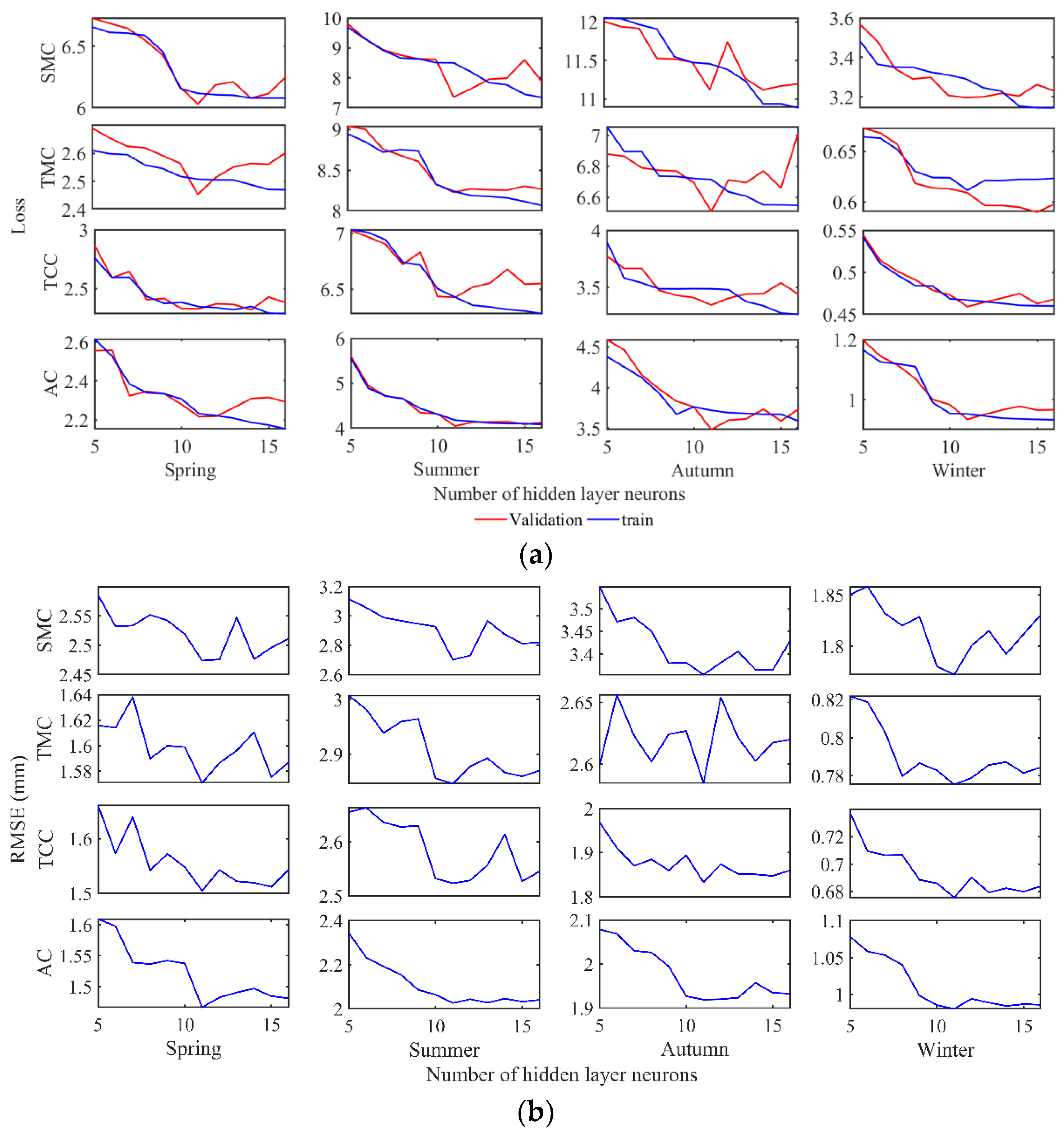In this study, m and n were set to 5 and 1, respectively; therefore, it can be determined that the optimal value of the hidden layer neurons was in the range of 5–11, which could be confirmed using an enumeration method [42]. At the same time, in order to avoid overfitting of model parameters, MSE was selected as the loss function to measure BPNN, and the range of hidden layer neurons was extended to 5–16 for verification. In addition, this paper used the trained model to correct the same external verification data, and further optimized the number of neurons in the hidden layer using the RMSEs. Since mainland China was divided according to climate types and seasons at the beginning of modeling, this could have led to differences in the number of neurons in the hidden layer of different models. Therefore, different models were built for testing in different regions and seasons. Here, 70% of the data were used for model training, 15% of the data were used for internal validation precision, and the remaining 15% of the data were used for outside precision verification.

As shown in Figure 5a, with the increase in the number of hidden layer neurons, the loss of the training set of all models decreased, while the loss of the validation set decreased first and then increased. This is because the increase in the number of hidden layer neurons gradually improved the fitting ability of the model for samples of the training set, but had side-effects on the prediction of unknown data due to overfitting. Statistics show that most models had the smallest loss in the validation set when the number of neurons in the hidden layer was 11. In the summer of the TCC region and spring of the AC region, when the number of neurons in the hidden layer was 11 or 12, the verification set loss was the smallest.

Figure 5b is the result of external test data correction using the trained models of different hidden layer neurons. Figure 6 is the result of external test data correction using the trained models of different hidden layer neurons. The RMSE corrected by the seasonal models for external data decreased first and then increased, and the minimum value was obtained when the number of neurons in the hidden layer was 11. Combined with the above verification by the loss function, the optimal number of neurons in the hidden layer was determined to be 11.

4.2. BPNN Model Based at Temporal Scale

The temporal scale-based BPNN model used the GNSS PWV provided by CMONOC from 2017–2018 and the corresponding ERA5 PWV to establish a fusion model and used the data from 2019 to test the model. The results are shown in

Table 3. Comparison of the ERA5 PWV and GNSS PWV before and after model fusion.

Climate Type	Season	Bias (mm)		RMSE (mm)		Correlation
		Before	After	Before	After	Before	After
SMC	Spring	0.35	−0.13	2.30	2.01	0.96	0.99
	Summer	1.27	0.09	3.27	2.72	0.92	0.99
	Autumn	0.86	0.25	2.62	2.28	0.98	0.99
	Winter	0.09	0.10	1.52	1.41	0.93	0.99
TMC	Spring	0.46	0.13	1.59	1.39	0.98	0.99
	Summer	−0.09	−0.24	2.95	2.60	0.97	0.99
	Autumn	−0.52	−0.07	1.79	1.57	0.98	0.99
	Winter	−0.38	0.01	0.87	0.69	0.94	0.99
TCC	Spring	−0.17	0.12	1.65	1.32	0.96	0.99
	Summer	1.35	0.04	2.92	2.25	0.92	0.99
	Autumn	0.24	0.11	1.77	1.49	0.97	0.99
	Winter	0.02	0.02	0.84	0.72	0.88	0.99
AC	Spring	1.12	0.15	2.02	1.36	0.92	0.99
	Summer	2.39	0.35	3.39	1.97	0.91	0.99
	Autumn	1.25	0.24	2.22	1.44	0.95	0.99
	Winter	0.31	0.03	1.12	0.89	0.8	0.99

and Figure 6 and Figure 7.

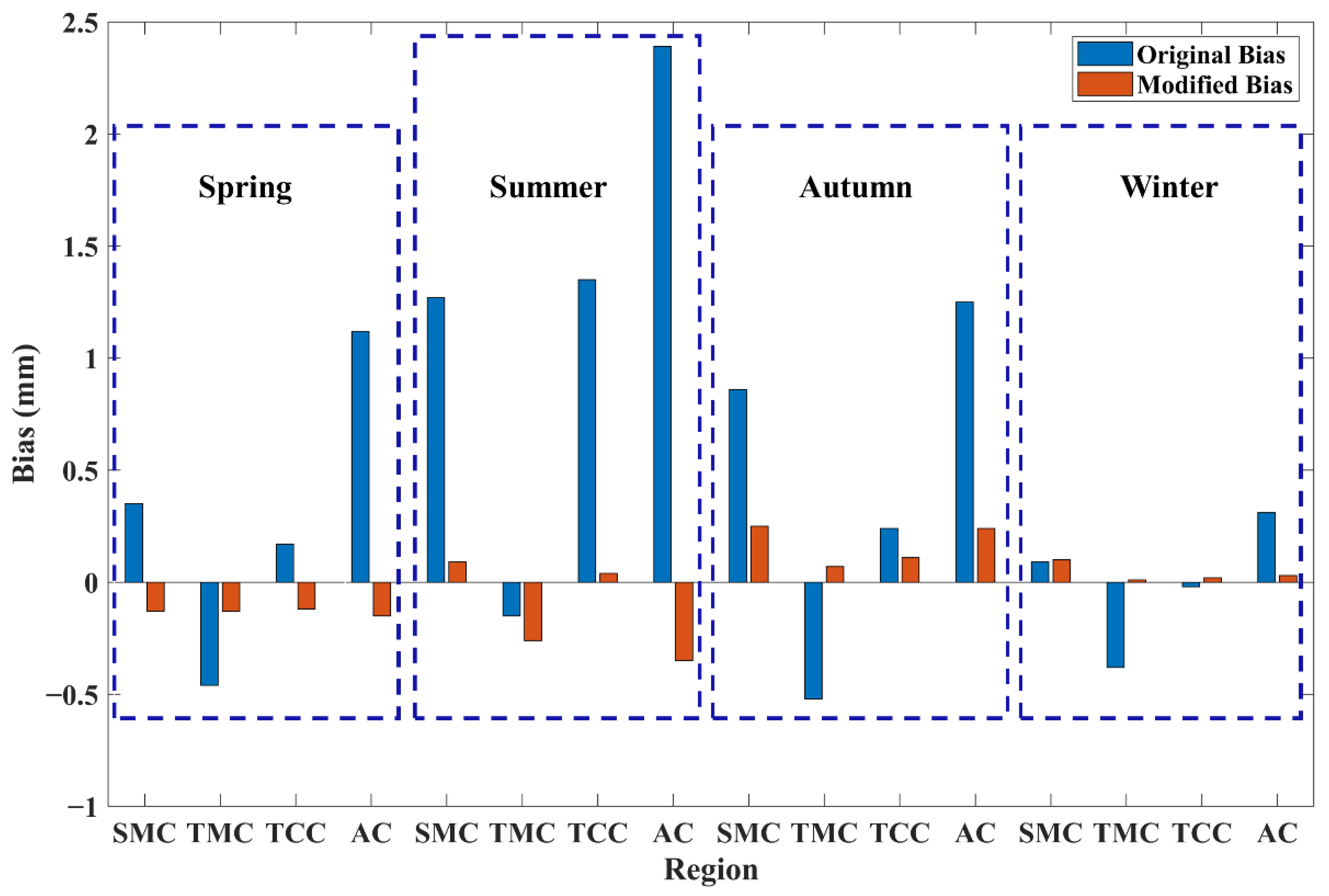
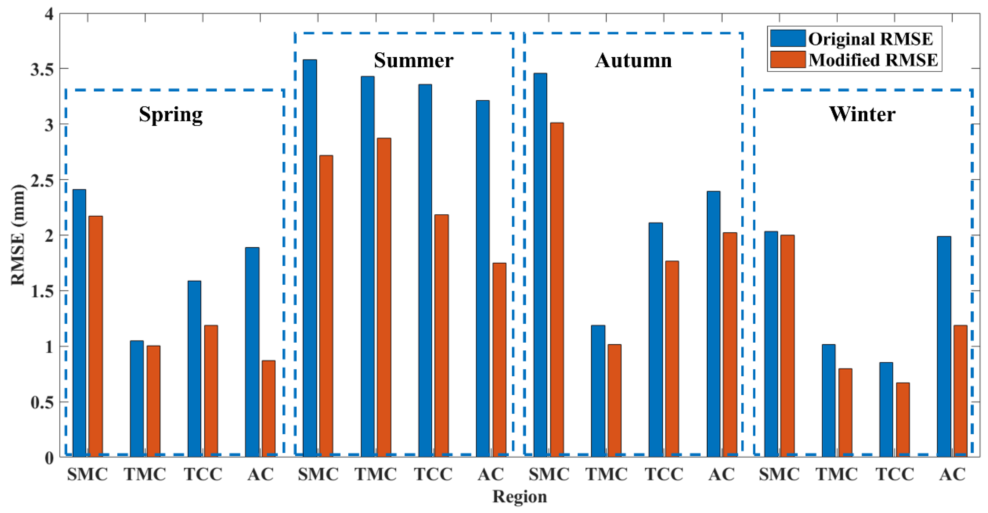
As shown in Table 2 and Figure 6, after the correction of the fusion model, the absolute bias of the ERA5 PWV in each period was less than 0.4 mm, which mainly fluctuated near 0. Figure 7 shows the RMSE of different regions in all time periods before and after the model calibration. Overall, the RMSE of the ERA5 PWV decreased from 2.05 mm to 1.67 mm, an improvement of 18.54%. The average overall RMSE decline in each season was 0.37 mm (spring), 0.74 mm (summer), 0.41 mm (autumn), and 0.16 mm (winter), and the corresponding improvement rates were 10.62%, 18.76%, 15.68%, and 13.49%, respectively. The RMSE of each region decreased by 0.33 mm (SMC), 0.23 mm (TMC), 0.35 mm (TCC), and 0.78 mm (AC), and the corresponding improvement rates were 10.62%, 12.19%, 13.57%, and 27.33%, respectively. At the same time, the correlation coefficient between the corrected ERA5 PWV and GNSS PWV increased to 0.99. The above statistical data show the applicability of the model at the temporal scale, especially for the summer with a larger RMSE and the AC area with poor accuracy. 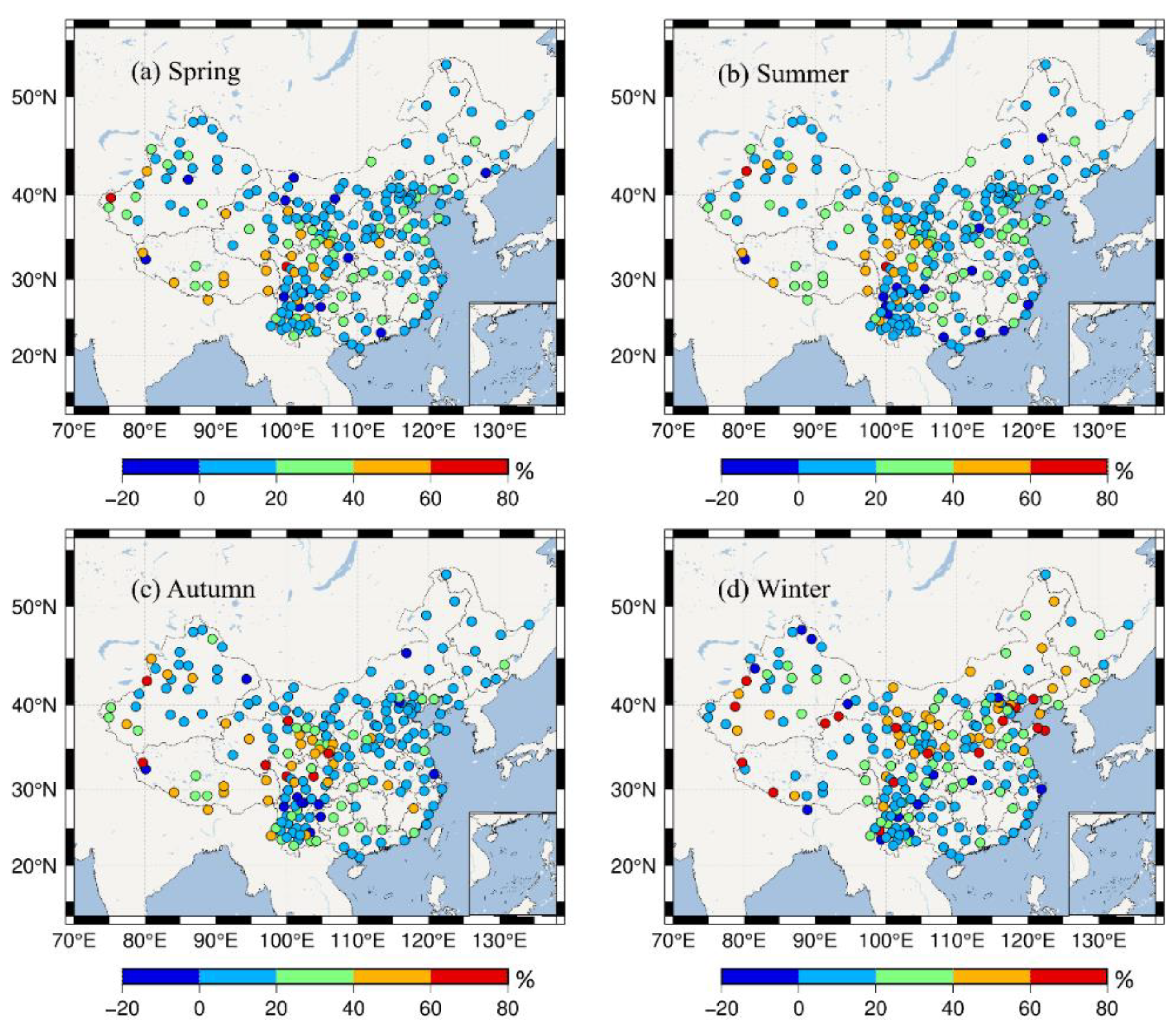Figure 8 also shows the correction rate of the ERA5 PWV after correction at each station.

As shown in Figure 8, the RMSE of the corrected ERA5 PWV and GNSS PWV was well corrected at most stations. The positive improvement rates in each season were 95% (spring), 94% (summer), 95% (autumn), and 94% (winter), with an average of 95%. The improvement rate was mainly concentrated in the 0–40% range, and the stations with an improvement rate of more than 40% were mainly concentrated in the central region of mainland China. The stations in this region were dense and could provide more mapping relationships between input and output, thus obtaining better improvement. A few stations showed worse results, accounting for approximately 5%, concentrated in mountainous areas with complex borders and geographical conditions in mainland China, but the average reduction rate was less than 7%. The above data show that the fusion model could effectively improve the ERA5 PWV at a temporal scale.

4.3. BPNN Model Based on Spatial Scale

From the above experiments, it can be seen that the model effectively improved the ERA5 PWV at a temporal scale, but this was based on the mapping input of the GNSS PWV and ERA5 PWV at all verification stations. In practice, the uneven distribution of GNSS stations leads to a lack of corresponding mapping input in some regions. Whether a regional model established at this time is still applicable at a spatial scale has not been verified, and some previous studies also lacked such a discussion. Therefore, 80% of the stations in the four regions were randomly selected for modeling, and the remaining 20% of the stations were selected for accuracy verification. The station selection is shown in Figure 9.

Figure 10 shows the biases of the original ERA5 PWV and the modified ERA5 PWV. The BPNN model significantly reduced the bias between the ERA5 PWV and the GNSS PWV of each validation station.

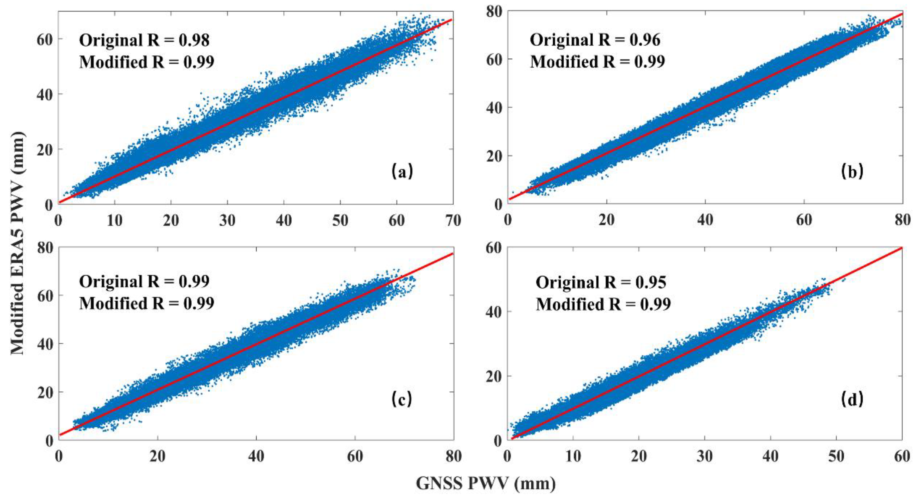
Figure 11 shows the scatterplot distribution of the ERA5 PWV and GNSS PWV in different seasons after the modification of the SMC regional verification station (only the SMC area is shown to reduce space). Compared with the ERA5 PWV before the correction, the correlation between the two was increased to 0.99.

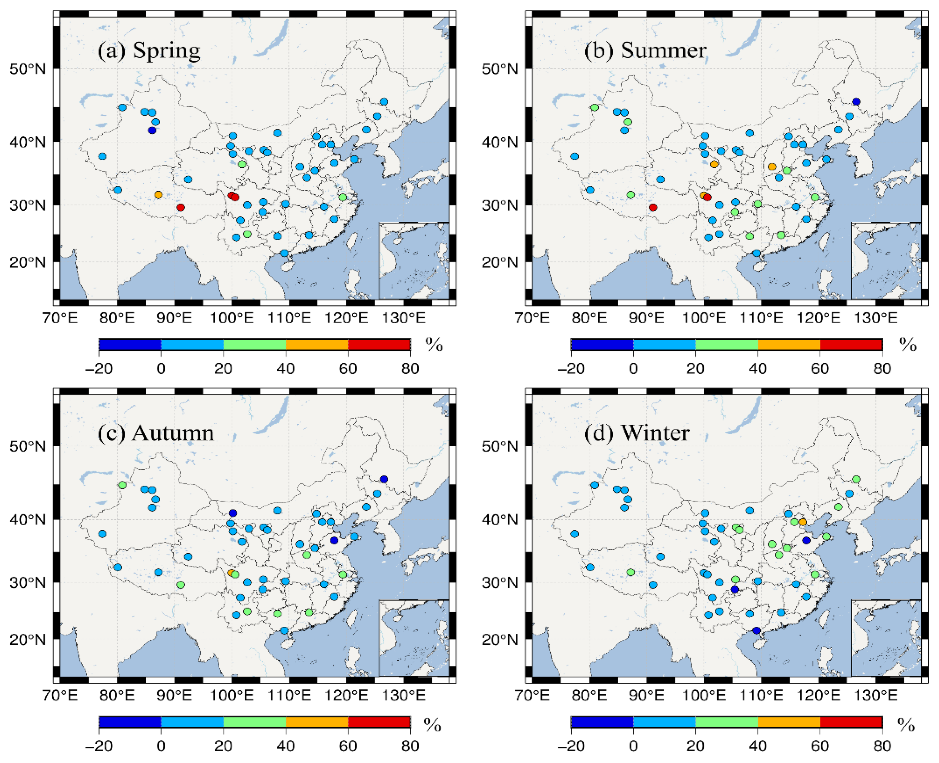
Figure 12 shows the improvement rate of the RMSE of the modified ERA5 PWV. From the regional perspective, the proportion of positive improvement in each region was 96% (SMC), 91% (TMC), 96% (TCC), and 100% (AC). The average improvement rate was more than 95%, and the corresponding RMSEs could be reduced by 0.26–38.65%, 0.49–42.31%, 0.28–46.87%, and 0.51–80%. Among the four regions, the BPNN model had the best correction for the AC region, which is not only a complex terrain with high altitude and less distribution of GNSS stations, but also a hot area for scientific research, which is conducive to further exploration of this region. From the perspective of the season, the proportions of positive improvement were as follows: 98% (spring), 98% (summer), 93% (autumn), and 93% (winter). The average improvement rate was more than 95%, and the corresponding RMSEs were reduced by 0.26–80%, 0.28–70.71%, 0.28–45.23%, and 0.30–40.75%. Among the four seasons, the BPNN model had the best correction effect in summer, while the previous research results showed that the ERA5 PWV had the worst performance in summer, which is a good improvement of the modified model. In addition, a few stations showed negative correction, but these stations were distributed along the edge of mainland China or in mountainous areas with complex topography and altitude, and the average negative correction rate was less than 5%. These statistics further illustrate the good applicability of the BPNN model at the spatial scale.

5. Generation of Modified ERA5 PWV Products

The construction and reliability of the above modified models were based on single-site data without taking advantage of the high spatial resolution of the ERA5 PWV data. Therefore, in this section, the correction model was applied to the correction of the ERA5 PWV as a whole to improve its accuracy on the basis of ensuring its high resolution. The regional climate fusion model was established using all station data from 2017 to 2019, and it was applied to the ERA5 PWV correction as a whole to obtain the corrected ERA5 PWV products. Due to space constraints, the modified ERA5 PWV distribution is shown only at 6:00 p.m. (UTC) on 23 January, 23 April, 29 August, and 23 October (Figure 13). To verify the accuracy of the products, we extracted ERA5 PWV using the same coordinates as the GNSS stations. Taking the above four timepoints as an example, the RMSE before and after calibration was calculated, as shown in Figure 14.

It can be seen from Figure 13 to Figure 14 that, after model correction, the RMSE of each region decreased to varying degrees. The calibration effect of the model was most obvious in summer, because the RMSE between the original ERA5 PWV and GNSS PWV was larger in this season, and it was easier to obtain good calibration results. The model also showed good applicability in the areas with large RMSE of AC and SMC, which effectively reduced the RMSE between them.

In addition, we evaluated the correction effect of the fusion model on ERA5 PWV at different elevations.

As shown in Figure 15, in the height range of 2600–2800 m, the maximum improvement of RMSE occurred in four seasons, which was related to the low accuracy of ERA5 PWV in the height range, and the error was well corrected by the fusion model. In spring and winter, the RMSE of ERA5 PWV was no more than 0.6 mm (except in spring in the elevation range of 2600–2800 m), which was related to the low PWV content in this time period. In summer, when the height was 1600–3000 m, the improvement of RMSE was significantly improved. On the one hand, the PWV content in summer was large, and the precipitation increased, leading to the rapid change of PWV. On the other hand, these stations were concentrated in the AC area where the height changes greatly; thus, the performance of ERA5 PWV in this area was poor. Therefore, the RMSE was greatly improved by model calibration. When the height was more than 3000 m, the improvement of RMSE began to weaken, because the temperature decreased rapidly with the increase in height, resulting in a decrease in PWV content. In autumn, the correction of the fusion model improved when the height exceeded 2000 m. The reason is that the PWV content was still high in this season, but the precipitation events were reduced, and the accuracy of ERA5 PWV in this height range was mainly related to the topographic fluctuations. Therefore, its improvement on RMSE in the height range larger than 3000 m was still significant.

6. Conclusions

Data fusion methods are the main method used to obtain high-precision and high-spatiotemporal-resolution PWV products. Most existing studies have some shortcomings while realizing their functions. Some methods ignore the error distribution law of in the overall modeling, some methods have high operation complexity, which is not conducive to their promotion, and most methods lack effective discussion on the spatial applicability of the model. Therefore, this study established a BPNN fusion model based on the distribution law of the PWV error and discussed the applicability of the model at the temporal and spatial scales.

This study first analyzed the distribution of the PWV in mainland China and the error distribution of the ERA5 PWV. The results showed that the distribution of the PWV in mainland China was mainly related to geographical location and climatic factors. The PWV content was the highest in the SMC area, followed by the TMC, TCC, and AC areas. There were also differences in the performance of the ERA5 PWV in mainland China. It was underestimated in the SMC, TCC, and AC areas, but overestimated in the TMC area. The RMSE was the largest in the SMC region and the smallest in the TCC region, related to the content of the PWV. The average correlation performance between the ERA5 PWV and GNSS PWV was above 0.9, with the highest in the TMC region and the lowest in the AC region. At the same time, the maximum RMSEs of ERA5 PWV and GNSS PWV in different seasons both appeared in summer, and the minimum appeared in winter.

On the basis of the temporal and spatial distribution of the PWV and the distribution law of the ERA5 PWV error, this study constrained the PWV, established a BPNN fusion model based on climate types and different seasons, and verified its applicability at temporal and spatial scales. The results showed that, compared with the original ERA5 PWV, the bias of PWV products generated using the fusion model decreased as a whole, and the correlation with the GNSS PWV increased to 0.99. The positive improvement rate of the RMSE reached 95%. At the temporal scale, the RMSE of the ERA5 PWV decreased from 2.05 mm to 1.67 mm, increasing by 18.54%. At the spatial scale, the RMSE decreased by 0.26–80% (spring), 0.28–70.71% (summer), 0.28–45.23% (autumn), and 0.30–40.75% (winter) in the four seasons. It is worth mentioning that the model had a 100% positive improvement in station verification in the AC area, and the model also exhibited suitable stability for the summer with the largest RMSE of the ERA5 PWV. In addition, the overall application of the model to the ERA5 PWV could improve the accuracy of ERA5 PWV products with guaranteed spatial resolution.

Furthermore, the fusion model reduces the workload required for establishing the model, is less time-consuming, and is simple to operate, which is beneficial for researchers to carry out additional related research.

Although the accuracy of ERA5 PWV in each region was well corrected by the BPNN fusion model, a large amount of data was needed as support, because the neural network needs sufficient training data to avoid the model falling into overfitting. We will explore a simpler method to calibrate ERA5 PWV products in a future study [43].

References

- Chen, B.; Liu, Z. Global water vapor variability and trend from the latest 36year (1979 to 2014) data of ECMWF and NCEP Reanalysis, radiosonde, GPS, and microwave satellite. J. Geophys. Res. Atmos. 2016, 121, 11442–11462. [Google Scholar] [CrossRef]
- Held, I.M.; Soden, B.J. Water vapor feedback and global warming. Annu. Rev. Energy Environ. 2000, 25, 441–475. [Google Scholar] [CrossRef] [Green Version]
- Dessler, A.E.; Sherwood, S.C. A matter of humidity. Science 2009, 323, 1020–1021. [Google Scholar] [CrossRef] [PubMed]
- Yao, Y.; Shan, L.; Zhao, Q. Establishing a method of short-term rainfall forecasting based on GNSS-derived PWV and its application. Sci. Rep. 2017, 7, 12465. [Google Scholar] [CrossRef]
- Chahine, M.T. The hydrological cycle and its influence on climate. Nature 1992, 359, 373–380. [Google Scholar] [CrossRef]
- Lee, S.W.; Kouba, J.; Schutz, B.; Kim, D.H.; Lee, Y.J. Monitoring precipitable water vapor in real-time using global navigation satellite systems. J. Geod. 2013, 87, 923. [Google Scholar] [CrossRef]
- Wang, S.; Xu, T.; Nie, W.; Jiang, C.; Yang, Y.; Fang, Z.; Li, M.; Zhang, Z. Evaluation of precipitable water vapor from five reanalysis products with ground-based GNSS observations. Remote Sens. 2020, 12, 1817. [Google Scholar] [CrossRef]
- Rocken, C.; Ware, R.; Van Hove, T.; Solheim, F.; Alber, C.; Johnson, J.; Bevis, M.; Businger, S. Sensing atmospheric water vapor with the global positioning system. Geophys. Res. Lett. 1993, 20, 2631–2634. [Google Scholar] [CrossRef] [Green Version]
- Chen, B.; Dai, W.; Liu, Z.; Wu, L.; Xia, P. Assessments of GMI-derived precipitable water vapor products over the south and east China seas using radiosonde and GNSS. Adv. Meteorol. 2018, 2018, 7161328. [Google Scholar] [CrossRef]
- Zhang, Q.; Ye, J.; Zhang, S.; Han, F. Precipitable Water Vapor Retrieval and Analysis by Multiple Data Sources: Ground-Based GNSS, Radio Occultation, Radiosonde, Microwave Satellite, and NWP Reanalysis Data. J. Sens. 2018, 2018, 3428303. [Google Scholar] [CrossRef]
- He, J.; Liu, Z. Comparison of satellite-derived precipitable water vapor through near-infrared remote sensing channels. IEEE Trans. Geosci. Remote Sens. 2019, 57, 10252–10262. [Google Scholar] [CrossRef]
- Sobrino, J.A.; Romaguera, M. Water-vapor retrieval from Meteosat 8/SEVIRI observations. Int. J. Remote Sens. 2008, 29, 741–754. [Google Scholar] [CrossRef]
- Gao, B.C.; Chan, P.K.; Li, R.R. A global water vapor data set obtained by merging the SSMI and MODIS data. Geophys. Res. Lett. 2004, 31, L18103. [Google Scholar] [CrossRef]
- Shi, F.; Xin, J.; Yang, L.; Cong, Z.; Liu, R.; Ma, Y.; Wang, Y.; Lu, X.; Zhao, L. The first validation of the precipitable water vapor of multisensor satellites over the typical regions in China. Remote Sens. Environ. 2018, 206, 107–122. [Google Scholar] [CrossRef]
- Shi, H.; Zhang, R.; Nie, Z.; Li, Y.; Chen, Z.; Wang, T. Research on variety characteristics of mainland China troposphere based on CMONOC. Geod. Geodyn. 2018, 9, 411–417. [Google Scholar] [CrossRef]
- Braun, J.; Rocken, C.; Ware, R. Validation of line-of-sight water vapor measurements with GPS. Radio Sci. 2016, 36, 459–472. [Google Scholar] [CrossRef] [Green Version]
- Zhao, Q.; Du, Z.; Yao, W.; Yao, Y. Hybrid precipitable water vapor fusion model in China. J. Atmos. Sol.-Terr. Phys. 2020, 208, 105387. [Google Scholar] [CrossRef]
- Zhang, Y.; Cai, C.; Chen, B.; Dai, W. Consistency evaluation of precipitable water vapor derived from ERA5, ERA-Interim, GNSS, and radiosondes over China. Radio Sci. 2019, 54, 561–571. [Google Scholar] [CrossRef]
- Wang, Y.; Yang, K.; Pan, Z.; Qin, J.; Chen, D.; Lin, C.; Chen, Y.; Tang, W.; Han, M. Evaluation of precipitable water vapor from four satellite products and four reanalysis datasets against GPS measurements on the southern Tibetan Plateau. J. Clim. 2017, 30, 5699–5713. [Google Scholar] [CrossRef]
- Zhao, Q.; Du, Z.; Li, Z.; Yao, W.; Yao, Y. Two-Step Precipitable Water Vapor Fusion Method. IEEE Trans. Geosci. Remote Sens. 2021, 60, 5801510. [Google Scholar] [CrossRef]
- Liu, X.; Wang, Y.; Huang, J.; Yu, T.; Jiang, N.; Yang, J.; Zhan, W. Assessment and calibration of FY-4A AGRI total precipitable water products based on CMONOC. Atmos. Res. 2022, 271, 106096. [Google Scholar] [CrossRef]
- Xiong, Z.; Zhang, B.; Sang, J.; Sun, X.; Wei, X. Fusing Precipitable Water Vapor Data in China at Different Timescales Using an Artificial Neural Network. Remote Sens. 2021, 13, 1720. [Google Scholar] [CrossRef]
- Zhang, B.; Yao, Y. Precipitable water vapor fusion based on a generalized regression neural network. J. Geod. 2021, 95, 1–14. [Google Scholar] [CrossRef]
- Bai, J.; Lou, Y.; Zhang, W.; Zhou, Y.; Zhang, Z.; Shi, C. Assessment and calibration of MODIS precipitable water products based on GPS network over China. Atmos. Res. 2021, 254, 105504. [Google Scholar] [CrossRef]
- Bei, L.I.U.; Yong, W.A.N.G.; Zesheng, L.O.U.; Wei, Z.H.A.N. The MODIS PWV correction based on CMONOC in Chinese mainland. Acta Geod. Et Cartogr. Sin. 2019, 48, 1207. [Google Scholar] [CrossRef]
- Alshawaf, F.; Fersch, B.; Hinz, S.; Kunstmann, H.; Mayer, M.; Meyer, F.J. Water vapor mapping by fusing InSAR and GNSS remote sensing data and atmospheric simulations. Hydrol. Earth Syst. Sci. 2015, 19, 4747–4764. [Google Scholar] [CrossRef] [Green Version]
- Alshawaf, F.; Hinz, S.; Mayer, M.; Meyer, F.J. Constructing accurate maps of atmospheric water vapor by combining interferometric synthetic aperture radar and GNSS observations. J. Geophys. Res. Atmos. 2015, 120, 1391–1403. [Google Scholar] [CrossRef]
- Li, X.; Long, D. An improvement in accuracy and spatiotemporal continuity of the MODIS precipitable water vapor product based on a data fusion approach. Remote Sens. Environ. 2020, 248, 11966. [Google Scholar] [CrossRef]
- Ma, X.; Yao, Y.; Zhang, B.; Yang, M.; Liu, H. Improving the accuracy spatial resolution of precipitable water vapor dataset using a neural network-based downscaling method. Atmos. Environ. 2022, 269, 118850. [Google Scholar] [CrossRef]
- Wu, M.; Jin, S.; Li, Z.; Cao, Y.; Ping, F.; Tang, X. High-precision GNSS PWV and Its variation characteristics in China based on individual station meteorological data. Remote Sens. 2021, 13, 1296. [Google Scholar] [CrossRef]
- Zhao, Q.; Yao, Y.; Yao, W.; Zhang, S. GNSS-derived PWV and comparison with radiosonde and ECMWF ERA-Interim data over mainland China. J. Atmos. Sol.-Terr. Phys. 2019, 182, 85–92. [Google Scholar] [CrossRef]
- Xu, J.; Meng, L.; Ren, C.; Xu, J. Analysis of mapping function in troposphere delay correction. J. Geod. Geodyn. 2008, 28, 120–124. [Google Scholar] [CrossRef]
- Bevis, M.; Businger, S.; Herring, T.A.; Rocken, C.; Anthes, R.A.; Ware, R.H. GPS meteorology: Remote sensing of atmospheric water vapor using the global positioning system. J. Geophys. Res. Atmos. 1992, 97, 15787–15801. [Google Scholar] [CrossRef]
- Hersbach, H.; Bell, B.; Berrisford, P.; Hirahara, S.; Horányi, A.; Muñoz-Sabater, J.; Nicolas, J.; Peubey, C.; Radu, R.; Schepers, D.; et al. The ERA5 global reanalysis. Q. J. R. Meteorol. Soc. 2020, 146, 1999–2049. [Google Scholar] [CrossRef]
- Hoffmann, L.; Günther, G.; Li, D.; Stein, O.; Wu, X.; Griessbach, S.; Heng, Y.; Konopka, P.; Müller, R.; Vogel, B.; et al. From ERA-Interim to ERA5: The considerable impact of ECMWF’s next-generation reanalysis on Lagrangian transport simulations. Atmos. Chem. Phys. 2019, 19, 3097–3124. [Google Scholar] [CrossRef] [Green Version]
- Dee, D.P.; Uppala, S.M.; Simmons, A.J.; Berrisford, P.; Poli, P.; Kobayashi, S.; Andrae, U.; Balmaseda, M.A.; Balsamo, G.; Bauer, D.P.; et al. The ERA-Interim reanalysis: Configuration and performance of the data assimilation system. Q. J. R. Meteorol. Soc. 2011, 137, 553–597. [Google Scholar] [CrossRef]
- Jiang, C.; Xu, T.; Wang, S.; Nie, W.; Sun, Z. Evaluation of Zenith Tropospheric Delay Derived from ERA5 Data over China Using GNSS Observations. Remote Sens. 2020, 12, 663. [Google Scholar] [CrossRef] [Green Version]
- Gardner, M.W.; Dorling, S. Artificial neural networks (the multilayer perceptron)—a review of applications in the atmospheric sciences. Atmos. Environ. 1998, 32, 2627–2636. [Google Scholar] [CrossRef]
- Reich, S.L.; Gomez, D.R.; Dawidowski, L.E. Artificial neural network for the identification of unknown air pollution sources. Atmos. Environ. 1999, 33, 3045–3052. [Google Scholar] [CrossRef]
- Sun, Z.; Zhang, B.; Yao, Y. Improving the estimation of weighted mean temperature in China using machine learning methods. Remote Sens. 2021, 13, 1016. [Google Scholar] [CrossRef]
- Wang, L.; Zeng, Y.; Chen, T. Back propagation neural network with adaptive differential evolution algorithm for time series forecasting. Expert Syst. Appl. 2015, 42, 855–863. [Google Scholar] [CrossRef]
- Cui, Y.; Long, D.; Hong, Y.; Zeng, C.; Han, Z. Validation and reconstruction of FY-3B/MWRI soil moisture using an artificial neural network based on reconstructed MODIS optical products over the Tibetan Plateau. J. Hydrol. 2016, 543, 242–254. [Google Scholar] [CrossRef]
- Zador, A.M. A critique of pure learning and what artificial neural networks can learn from animal brains. Nat. Commun. 2019, 10, 3770. [Google Scholar] [CrossRef] [PubMed] [Green Version]
Figure 1.
Geographical distribution of Crustal Movement Observation Network of China (CMONOC) GNSS stations in different climate types. SMC represents the subtropical monsoon climate region, TMC represents the temperate monsoon climate region, TCC represents the temperate continental climate region, and AC represents the plateau mountain climate region.
Figure 2.
Structure of the BPNN model.
Figure 3.
(a) Annual average PWV value at GNSS stations. (b–d) Bias, RMSE, and correlation between the GNSS PWV and ERA5 PWV, respectively.
Figure 4.
Distribution of the average PWV in different seasons and the RMSE distribution of the ERA5 PWV. (a,c,e,g) represent the average PWV in spring, summer, autumn and winter respectively, (b,d,f,h) are the corresponding RMSE distributions.
Figure 5.
(a). Model training and validation loss of the BPNN model under different numbers of hidden layer neurons. (b). RMSE of the BPNN model under different numbers of hidden layer neurons.
Figure 6.
Comparison of the bias between the original ERA5 PWV and modified ERA5 PWV.
Figure 7.
Comparison of the RMSE between the original ERA5 PWV and modified ERA5 PWV.
Figure 8.
Distribution of the improvement rates of all verification stations in different seasons at time scales.
Figure 9.
Distribution of modeling and verification stations. Blue spots were used for modeling, while red spots were used for external validation.
Figure 10.
PWV biases at verification stations of the original ERA5 PWV and the modified ERA5 PWV.
Figure 11.
SMC regional validation station ERA5 PWV and GNSS PWV scatter plots. (a–d) Spring, summer, autumn, and winter, respectively.
Figure 12.
Distribution of the improvement rates of all verification stations in different seasons at spatial scales.
Figure 13.
The distribution of PWV before (a,c,e,h) and after (b,d,f,g) calibration at 6:00 p.m. (UTC) on 23 January, 23 April, 29 August, and 23 October.
Figure 14.
Comparison of RMSE between ERA5 PWV and GNSS PWV before and after calibration.
Figure 15.
RMSE improvement at different heights.