Performance Evaluation of Interest Point Detectors for Heterologous Image Matching

Abstract

In point-based heterologous image matching algorithms, high-quality interest point detection directly affects the final image matching quality. In this paper, starting from the detection mechanism of each interest point detector, optical images and SAR images with different resolutions and covering different areas are selected as experimental data. The five state-of-the-art SAR-Harris, UND-Harris, Har-DoG, Harris-Laplace and DoG interest point detectors are analyzed in terms of scale difference adaptability, nonlinear intensity difference adaptability, distribution uniformity, image registration alignment performance and detection efficiency. Then, we performed registration experiments on images from different sensors, at different times, and at different resolutions to further validate our evaluation results. Finally, the applicable image types of each detector are summarized. The experimental results show that SAR-Harris has the best performance in scale difference adaptability, and UND-Harris has the weakest performance. In terms of nonlinear intensity difference adaptability, SAR-Harris and UND-Harris are comparable, and DoG performance is the weakest. The distribution uniformity of UND-Harris is significantly better than other detectors. Although Har-DoG is weaker than Har-Lap and DoG in repeatability, it is better than both in final image alignment performance. DoG is superior in detection efficiency, followed by SAR-Harris. A comprehensive evaluation and a large amount of experimental data are used to evaluate and summarize each detector in detail. This paper provides a useful guide for the selection of interest point detectors during heterologous image matching.

1. Introduction

With the continuous development of synthetic aperture radar (SAR) imaging technology towards high resolution and wide swath, the application potential of SAR image data in many fields has gradually been reflected. Using high-precision heterogenous images as a reference, registering SAR images is a hot spot in the field of remote sensing image matching. Image matching is the geometric alignment of two or more images from the same area; usually, these images are obtained under different imaging conditions (different sensors, different imaging times, etc.). Matching methods are mainly divided into two types: intensity-based methods and feature-based methods [1]. Intensity-based methods usually adopt the idea of template matching. This involves selecting a template window on the reference image, and then searching within a certain search area on the image to be matched. The similarity measure (such as cross-correlation, mutual information, sum of squared differences, etc.) is calculated between the template window and the pixel intensity corresponding to the search area window on the image to be matched to obtain the peak value of the similarity measure function, and finally the matching position is determined. Feature-based methods consist of three steps: feature extraction, feature description, and feature matching. In the feature extraction stage, the common features between the two images should be detected as much as possible, and the types of these common features include point features, line features, and area features. Feature description is to generate feature descriptors (that is, feature vectors with a certain length) for the extracted features. The final feature matching is to find the same features by calculating the similarity measure (such as Euclidean distance) between the descriptors based on the feature descriptors, and estimate the image transformation matrix.

The advantage of the intensity-based method is that only the corresponding simi-larity measure needs to be selected, and additional feature detection and description are not required. However its disadvantage is also obvious; it needs to calculate the similarity measure of all pixels in the template window, which is very time-consuming. Due to the strong nonlinear intensity difference between heterologous images, the search surface becomes non-smooth, and it is easy to fall into the local optimal value during the search process. Therefore, it is not suitable for the matching of heterologous images. Compared with the former pixel-by-pixel calculation, the feature-based method only needs to detect some salient features in the image, so it can achieve higher efficiency than the former, and this method can easily achieve scale and rotation invariance. The disadvantage is that different feature extraction methods will have a greater impact on the final matching result, so for a specific application, choosing an appropriate feature extraction method is particularly important. In the feature-based method, the point feature is easier to locate accurately on the image than the line feature and the area feature, and its detection complexity is also lower than the latter. Therefore, the point-based matching method is currently the most widely used [1,2]. Point features include corner points and blob points, which correspond to different interest point detectors. In recent years, quite a few scholars have evaluated the performance of interest point detectors in different application fields.

In the field of computer vision, Zukal, M. et al., explored the influence of Harris, Hessian and DoG interest point detectors by illumination and histogram equalization [3]. Cordes, K. et al., analyzed the localization accuracy of alternative interest point detector (ALP) and DoG interest point detector, and the results show that ALP is better than DoG [4]. To verify the combined performance of different interest point detectors, Ehsan, S. et al., proposed an evaluation metric based on the spatial distribution of interest points, and extended it to provide a measure of complementarity of pairwise detectors. Experimental results show that the scale-invariant feature detectors dominate whether used alone or in combination with other detectors [5]. Ruby, P.D. et al., used the survival rate as the evaluation indicator to explore the detection performance of four classical interest point detectors under a series of image sequences such as rotation, scaling and blurring [6]. In addition to the repeatability, Barandiarán, I. et al., introduced two indicators, the number of interest points and the detection efficiency, and conducted a comprehensive evaluation of nine classical interest point detectors [7]. For specific applications, in order to explore the performance of interest point detectors in real-time visual tracking, Steffen, G. et al., designed a video sequence dataset containing various geometric changes, lighting changes and motion blur. Taking this dataset as a benchmark, they comprehensively analyze all relevant factors affecting real-time visual tracking by combining interest point detectors and feature descriptors [8]. In a simultaneous localization and mapping (SLAM) application, Gil, A. et al., evaluated the repeatability of interest point detectors and the invariance and saliency of descriptors on different 3D scene image sequences [9]. Prˇibyl et al., studied the performance of interest point detectors on high dynamic range (HDR) images, using interest point distribution and repeatability as indicators, and the results showed that current interest point detectors cannot handle HDR images well [10]. For HDR image processing, Melo, W.A. et al., proposed an improved interest point detector and tested with a large number of HDR images, finally verifying the effectiveness of the proposed algorithm [11]. Gunashekhar, P.K. et al., applied the contrast stretching technique to the multi-scale Harris and multi-scale Hessian detectors, and proved through experiments that the improved detectors have improved repeatability in terms of illumination, viewing angle, and scale [12]. Kazmi et al., conducted an experimental study on the performance of interest point detectors applied to image retrieval and classification. By combining detectors with descriptors, it was concluded that interest point detectors can achieve high accuracy in building recognition [13]. Molina et al., studied the performance of interest point detectors applied to infrared image and visible image face analysis. The experimental results show that compared with SIFT, ORB and BRISK, SURF shows better performance in terms of repeatability and accuracy [14].

Although a large number of researchers in the field of computer vision have evaluated the performance of many mainstream interest point detectors, the data used in their research are mainly close-range images or ordinary data camera images, and the main influencing factors are scale, viewing angle, lighting, and additive noise. In contrast to close-range images, heterologous remote sensing images are usually taken at high altitude, and the types of ground objects they cover are more complex. Due to the different imaging modes and imaging conditions of heterologous images, there are obvious geometric distortions and grayscale differences between images. This puts forward higher requirements on the performance of interest point detectors, which must be able to reflect the common features between images to the greatest extent. In the field of remote sensing image matching, Wang et al., used SSIM (Structural Similarity Image Measurement) and PSNR (Peak Signal to Noise, PSNR) as image quality metrics. The relationship between image quality and repeatability of interest point detector applied to remote sensing images is studied. The results show that the repeatability decreases as the image quality decreases, and under certain conditions this relationship can be modeled with some simple functions [15]. The following year, Ye et al., used remote sensing images as experimental data to evaluate the performance of mainstream interest point detectors in the computer vision field [16].

To the author’s knowledge, the comparative research on the performance of interest point detectors used in heterogeneous remote sensing image matching is relatively limited. In the existing research, the detector scope of its research does not include the latest research progress, and the evaluation indicators used are relatively single.

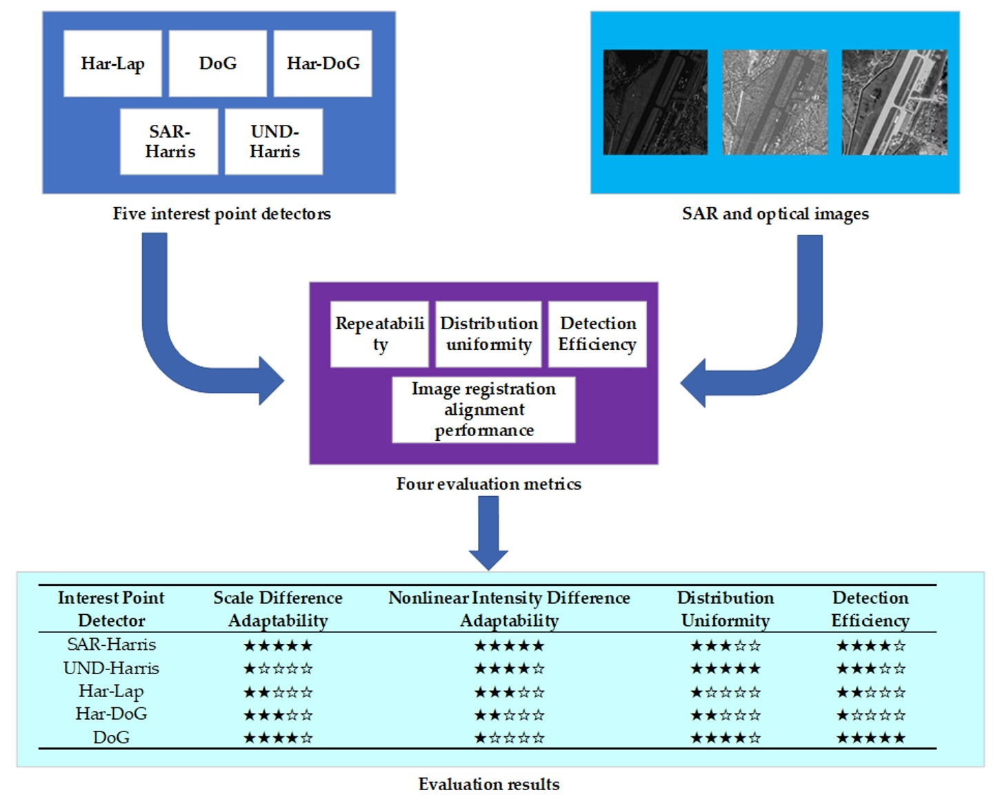
In this paper, optical images and SAR images are used as experimental data to evaluate the performance of interest point detectors in five aspects: scale difference adaptability, nonlinear intensity difference adaptability, distribution uniformity, image registration alignment performance and detection efficiency. Finally, we conduct comprehensive image registration experiments to further validate our evaluation results. Considering that SAR-Harris, UND-Harris and Har-DoG show good detection performance in the field of remote sensing image matching, as well as Harris-Laplace and DoG are widely used detectors in the field of computer vision [17]. Therefore, this paper will evaluate the performance of these five detectors.

2. Methodology

2.1. Interest Point Detectors

2.1.1. Harris-Laplace Detector

Harris-Laplace (Har-Lap) combines scale space theory and Harris corner detection detector to make scale invariant [18]. It uses the Harris function to detect corners in the scale space and uses the LoG operator [19] for scale localization. The interest point detection process is shown in Figure 1.

Firstly, Gaussian kernels of different scales (that is, different standard deviations) are used to continuously smooth the input image to obtain a Gaussian scale space. Then, the Harris function response is calculated in the image space of each layer scale image, as shown in the following equation:

$$\mathrm{h}=\det \left(M\left(\mathit{x},{\mathbf{\sigma }}_I,{\mathbf{\sigma }}_D\right)\right)-d\cdot tr{\left(M\left(\mathit{x},{\mathbf{\sigma }}_I,{\mathbf{\sigma }}_D\right)\right)}^2$$

(1)

Among them, M is the scale-adaptive second-order moment matrix of the image, that is

$$M\left(\mathit{x},{\mathbf{\sigma }}_I,{\mathbf{\sigma }}_D\right)={\mathbf{\sigma }}_D^2{G}_{{\sigma }_I}\ast \left[\begin{array}{cc}{L}_x^2\left(\mathit{x},{\mathbf{\sigma }}_D\right)& L_x{L}_y\left(\mathit{x},{\mathbf{\sigma }}_D\right)\\ L_x{L}_y\left(\mathit{x},{\mathbf{\sigma }}_D\right)& L_y^2\left(\mathit{x},{\mathbf{\sigma }}_D\right)\end{array}\right]$$

(2)

σ_D and σ_I are the differential and integral scales, respectively, and satisfy σ_D = 0.7σ_I. x represents the pixel coordinate vector of the image. L_x (x, σ_D) and L_x (x, σ_I) represent the first-order difference horizontal and vertical gradients of the pixel at the position in the Gaussian kernel blurred image with standard deviation σ_D, respectively. G_σI represents the Gaussian kernel with standard deviation σ_I, and ∗ is the convolution operation. Several corner points can be extracted by setting the Harris function response threshold. Finally, in order to obtain the scale attributes of the corner points, one needs to calculate the Laplacian-of-Gaussian (LoG) values of all scale layer images, and judge whether the LoG value of the scale where each corner point located is larger than the LoG values of the scales of the upper and lower layers; if the condition is met, the point is retained. The filtered corner points have the scale attribute. The corner points extracted by the Har-Lap detector are shown in Figure 2a.

2.1.2. DoG Detector

Differently from Har-Lap, DoG additionally performs corresponding down-sampling operations on the basis of smoothing with Gaussian kernels in order to satisfy the continuity of scale changes. The schematic diagram of the construction of DoG scale space is shown in Figure 3.

The Gaussian pyramid is divided into several octaves, and each octave contains several layers. Within each octave, Gaussian kernels with different standard deviations were used for blurring. Between different octaves, corresponding down-sampling operations are performed, and the first layer of the next octave is obtained by twice down-sampling the third-to-last layer of the previous octave. The difference of Gaussian scale (DoG) scale space is obtained by subtracting the Gaussian blurred images of two adjacent scales in the same octave. The extreme point detection is performed in the DoG space to obtain Blob points. The schematic diagram of extreme point detection is shown in Figure 4 [20].

Compare the pixel value of the extreme point to be detected with its current 8 neighbors on the DoG layer and the 18 neighbor pixel values of its upper and lower DoG layers (26 neighbors in total); if the point is a local extreme point (maximum or minimum), it is used as a candidate interest point for the next stage. Since DoG will generate a strong edge response, it is necessary to remove low-contrast extreme points and unstable edge response points on the basis of the previous step to obtain the final interest points. The interest points extracted by DoG are shown in Figure 2b.

2.1.3. Har-DoG Detector

Har-DoG is proposed by Ye, Y. on the basis of Har-Lap and DoG [21], which combines Har-Lap corner points and DoG Blob points. According to the condition that DoG is an approximation of LoG, DoG is used instead of LoG to complete the scale positioning in the process of corner detection, and Blob point detection can also be performed in DoG space. The overall detection process is divided into the following three steps:

Step 1: Construct Gaussian scale space and DoG scale space.

Step 2: Harris corner points detection is performed in the Gaussian scale space, and the scale of the corner is determined by the DoG response.

Step 3: Blob points detection in DoG space.

The interest points extracted by Har-DoG are shown in Figure 2c.

2.1.4. SAR-Harris Detector

SAR-Harris was proposed in the SAR-SIFT [22] algorithm. Aiming at the problem that the differential gradient operator is easily interfered by the multiplicative speckle noise when applied to the SAR image, the ROEWA operator is introduced to calculate the horizontal and vertical gradient.

$$G{R}_{x,{\alpha }_n}=\log \left(R_{x,{\alpha }_n}\right)$$

(3)

$$G{R}_{y,{\alpha }_n}=\log \left(R_{y,{\alpha }_n}\right)$$

(4)

where R_x,α and R_y,α are calculated by:

$$R_{x,{\alpha }_n}=\frac{{\displaystyle \sum _{i=-M/2}^{M/2}}{\displaystyle \sum _{j=1}^{N/2}}I(x+i,y+j)e^{-\frac{\left|i\right|+\left|j\right|}{{\alpha }_n}}}{{\displaystyle \sum _{i=-M/2}^{M/2}}{\displaystyle \sum _{j=-N/2}^{-1}}I(x+i,y+j)e^{-\frac{\left|i\right|+\left|j\right|}{{\alpha }_n}}}$$

(5)

$$R_{y,{\alpha }_n}=\frac{{\displaystyle \sum _{i=1}^{M/2}}{\displaystyle \sum _{j=-N/2}^{N/2}}I(x+i,y+j)e^{-\frac{|i+|\left|j\right|}{{\alpha }_n}}}{{\displaystyle \sum _{i=-M/2}}{\displaystyle \sum _{j=-N/2}^{N/2}}I(x+i,y+j)e^{-\frac{|i++|j\mid }{{\alpha }_n}}}$$

(6)

In the equation above, α_n is the corresponding scale factor, (x, y) represents the coordinate of the image pixel whose gradient needs to be calculated, M and N are the calculation window size of ROEWA operator, which are related to the scale factor α_n; the larger the α_n, the larger the window. Similar to Har-Lap, the first-order differential gradient is replaced by the ROEWA gradient to obtain the SAR-Harris function, which can be calculated by:

$$C_{\mathrm{SH}}(x,y,{\alpha }_n)=G_{\sqrt{2}\cdot {\alpha }_n}\ast \left[\begin{array}{cc}{\left(G{R}_{x,{\alpha }_n}\right)}^2& \left(G{R}_{x,{\alpha }_n}\right)\cdot \left(G{R}_{y,{\alpha }_n}\right)\\ \left(G{R}_{x,{\alpha }_n}\right)\cdot \left(G{R}_{y,{\alpha }_n}\right)& {\left(G{R}_{y,{\alpha }_n}\right)}^2\end{array}\right]$$

(7)

$$R_{\mathrm{SH}}(x,y,{\alpha }_n)=\det \left(C_{\mathrm{SH}}(x,y,{\alpha }_n)\right)-d\cdot tr{\left(C_{\mathrm{SH}}(x,y,{\alpha }_n)\right)}^2$$

(8)

In the above equation, $G_{\sqrt{2}{\alpha }_n}$ is a Gaussian kernel with a standard deviation of $\sqrt{2}$α_n. The interest points extracted by SAR-Harris are shown in Figure 2d.

2.1.5. UND-Harris Detector

The traditional multi-scale Harris detector relies on Gaussian blur, which suffers from two key drawbacks: (1) The Gaussian kernel used is isotropic, and different image geometric structures are blurred to the same degree. This may lead to a situation where some interest points that can be correctly matched cannot be extracted in the feature detection stage. (2) The extracted interest points cannot be evenly distributed in the image space. For images with local geometric distortion, the uneven distribution of interest points will reduce the quality of image matching.

The Harris interest point detector based on uniform nonlinear diffusion (UND-Harris) [23] uses nonlinear diffusion filtering instead of Gaussian filtering to better preserve the edge and detail information of the image while suppressing noise. The comparison between nonlinear diffusion filtering and Gaussian filtering is shown in Figure 5 below.

In order to make the extracted interest points evenly distributed in scale space and image space, feature scale and block strategy are introduced. The number of interest points for each scale layer is determined using the following equation:

$$N_m=N_{\mathrm{total}}·F_m,\sum _{m=1}^M{F}_m=1$$

(9)

Among them, N_total is the total number of interest points to be extracted, N_m is the number of interest points to be extracted for the m-th scale layer, and F_m is the ratio of m-th layer interest points number to the total number of interest points. F_m can be calculated by

$$\left\{\begin{array}{c}{F}_m=\frac{{\alpha }_1}{{\alpha }_m}{f}_1\hfill \\ f_1=1/{\displaystyle \sum _{m=0}^{M-1}}{c}^{-m},m=1,\dots ,M\hfill \\ {\alpha }_m={\alpha }_0·c^m\hfill \end{array}\right.$$

(10)

α₀ and α_m represent the initial scale and the scale corresponding to the m-th scale layer, respectively. C represents the ratio between the two scale layers. In order to make the interest points extracted in each scale layer evenly distributed in the image space, each scale layer is divided into n × n non-overlapping sub-blocks. The number of interest points to be extracted for each sub-block in the m-th scale layer is

$$h=\frac{N_m}{n^2}$$

(11)

In the actual extraction of interest points, the calculation of the corner response function and the setting of the threshold are consistent with the multi-scale Harris detector. The Harris response of each sub-block in the image of each scale layer is calculated separately, and h points with larger response intensities are selected as the interest points extracted in the sub-block.

2.2. Evaluation Metrics

2.2.1. Repeatability

For image matching applications, if the interest points detected in the reference image can also be detected in the sensed image, this is very beneficial for the subsequent matching process. Therefore, the repeatability of interest points is introduced as the performance indicator of interest point detectors. The higher the repeatability, the greater the possibility that the interest points can be correctly matched later [24,25]. The equation for calculating the interest point repeatability is as follows:

$$R=\frac{K}{\min (M,N)}$$

(12)

In the equation above, R is the repeatability, K represents the number of corresponding point pairs between two images. M and N are the number of interest points detected on the reference image and the sensed image, respectively, and these points must be located in the same area of two images. min (∙) represents the minimum operation. The equation for calculating M and N is:

$$M=\left\{num(P_i)|T\cdot P_i\in I_1\right\}$$

(13)

$$N=\left\{num(P_j)|T^{-1}\cdot P_j\in I_2\right\}$$

(14)

T represents the transformation matrix from the reference image to the sensed image. P_i and P_j represent the interest points in the reference image and the sensed image, respectively. min (∙) represents the number of interest points. I₁ and I₂ are the pixel coordinate ranges of the reference image and the sensed image, respectively.

For the discrimination of corresponding point pairs, it is necessary to restrict from the two criteria of position and scale.

(1) Location criteria

$$dist(P_j,T\cdot P_i)\le r$$

(15)

where r is the distance threshold, generally set to 1.5 pixels, dist (∙) represents the distance operator between two points.

(2) Scale criteria

When multi-scale interest point detection is performed in the scale space, the scale attribute of the corresponding point pairs should also be considered, and the scale difference between the corresponding point pairs in two images satisfies ε_s < 0.4, and

$${\epsilon }_s=\left|1-S^2\frac{\min ({\sigma }_i{}^2,{\sigma }_j{}^2)}{\max ({\sigma }_i{}^2,{\sigma }_j{}^2)}\right|$$

(16)

In the above equation, σ_i and σ_j are the scales corresponding to the two interest points respectively. S is the scale ratio of the two images (S ≥ 1).

2.2.2. Distribution Uniformity

Due to the local geometric distortion in the remote sensing image, if the corresponding point pairs are not uniformly distributed on the images (concentrated in some areas), the quality of the final image matching tends to be degraded [26]. Therefore, in the feature detection stage, the distribution uniformity of interest points is also an important indicator to evaluate the performance of interest point detectors. In this paper, the distribution uniformity [27] is introduced as a criterion for evaluating the spatial distribution of interest points on the image.

This criterion needs to complete three steps: (1). Image sub-region division; (2). Count the number of interest points in each sub-region, and calculate the variance of the number of interest points in ten sub-regions; (3). Calculate the distribution uniformity.

First, the image area is divided in five directions to obtain ten sub-areas, as shown in Figure 6 below, and the two sub-areas obtained by each division are equal in area.

Then, count the number of interest points in each sub-region N_{region_i}, i = 1, 2, …, 10. Normalize N_{region_i} and compute the standard deviation N_std as an indicator of distribution uniformity, The smaller N_std is, the more evenly the interest points are distributed.

2.2.3. Image Registration Alignment Performance

This is a subjective evaluation metric that matches heterologous images by com-bining interest point detectors with feature descriptors. The two registered images are superimposed to display the corresponding mosaic map, and the alignment performance at the junction of the images in the mosaic map is observed and qualitatively scored.

2.2.4. Detection Efficiency

Under the premise of detecting the same number of interest points, the less the detection time consumed by the detector, the higher the detection efficiency. By adjusting the detection threshold, the number of interest points detected by each detector is the same, and the time consumption of the detectors is calculated for comparison.

3. Experiments

3.1. Scale Difference Adaptation

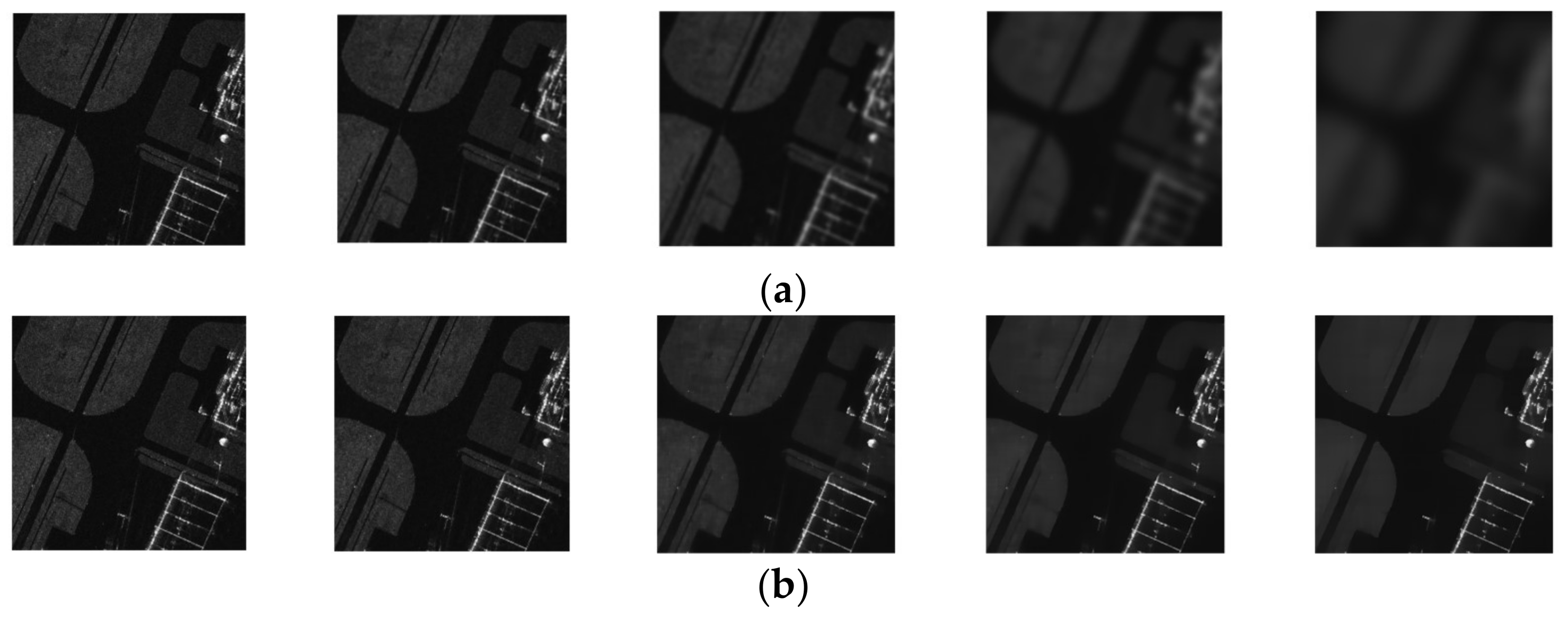
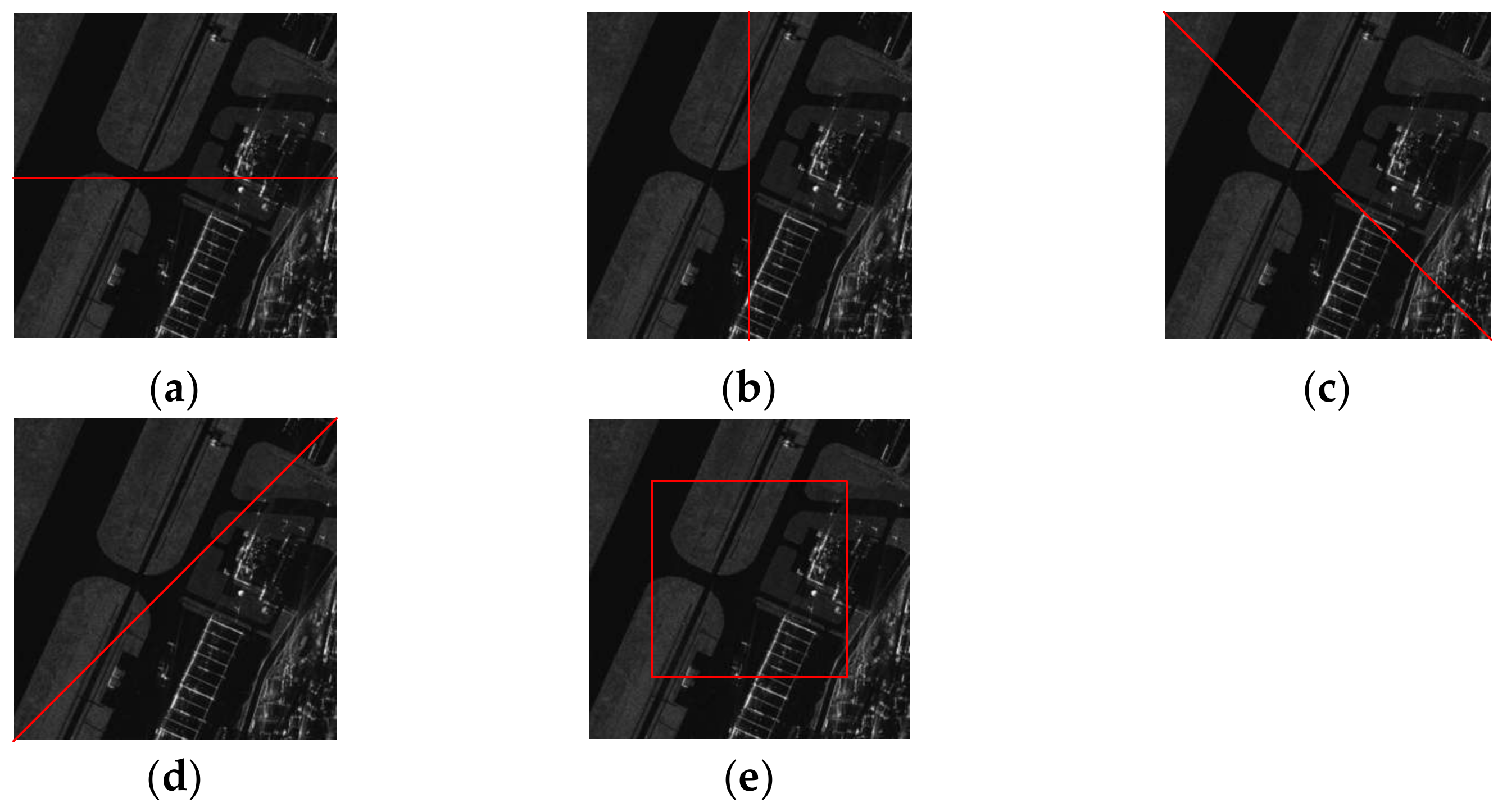
This group of experiments tests the adaptability of the interest point detector to the difference in image scale. Airborne high-resolution SAR images and spaceborne medium-resolution SAR images were selected, respectively. The images of both resolutions are located in an airport area; the high-resolution image has a resolution of 0.2 m and a size of 1300 × 1300. Medium resolution images have a resolution of 10 m and a size of 600 × 600. Each set of data contains five images, where the scale difference is achieved by manual scaling, taking 1.5, 2, 2.5, and 3 times the scale difference, respectively. The experimental data are shown in Figure 7 below.

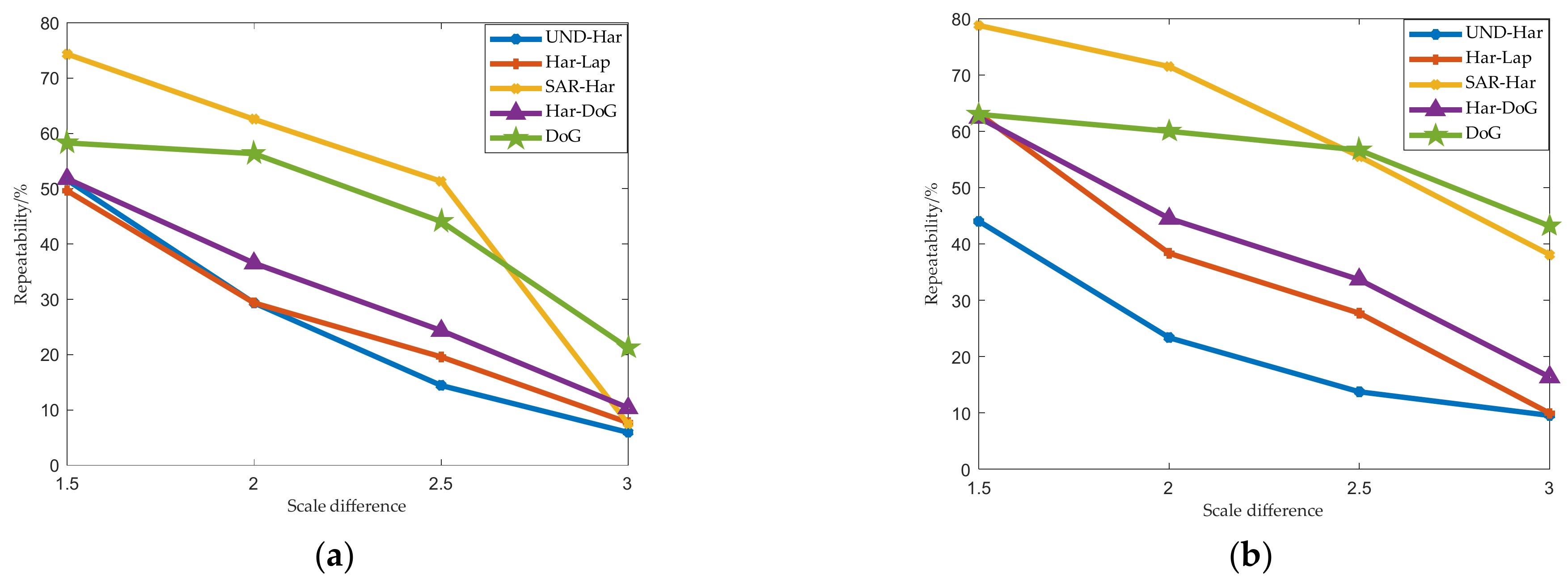
Figure 8 shows the repeatability of each interest point detector on the above data. As the scale difference increases, the repeatability of all detectors shows a monotonically decreasing trend. For images of two resolutions, among the five detectors, the repeatability of SAR-Harris is the highest compared with other detectors (when the scale difference is between 1.5 and 2.5). UND-Harris is the lowest. In addition, the repeatability of DoG is higher, followed by Har-DoG and Har-Lap.

3.2. Nonlinear Intensity Difference Adaptation

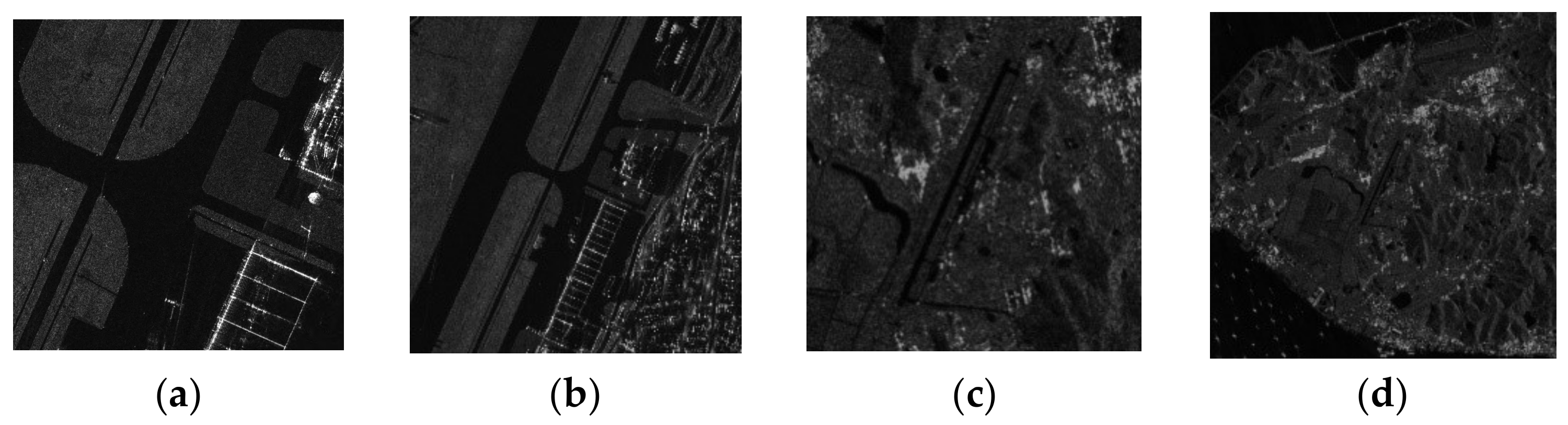
Due to the different imaging modes, there is a large nonlinear intensity difference between heterogeneous images. This group of experiments studies the adaptability of the interest point detector to this difference. The selected image data information is shown in

Table 1. Image pairs with Nonlinear intensity difference.

Area	Dataset Description
	Reference Image	Sensed Image	Image Characteristic
1	Sensor: GF-3	Sensor: Airborne SAR	The imagery covers an airport and its surrounding area. There is a significant intensity inversion between the optical image and the SAR image.
	GSD: 3 m	GSD: 3 m
	Size: 600 × 600	Size: 600 × 600
	Sensor: Google Earth	Sensor: Airborne SAR
	GSD: 1 m	GSD: 1 m
	Size: 1744 × 1541	Size: 1744 × 1541
	Sensor: Google Earth	Sensor: Airborne SAR
	GSD: 3 m	GSD: 3 m
	Size: 600 × 600	Size: 600 × 600
2	Sensor: GF-3	Sensor: Airborne SAR	The imagery covers an area of ponds, and all three types of images have a significant aggregate structure in this area.
	GSD: 3 m	GSD: 3 m
	Size: 600 × 600	Size: 600 × 600
	Sensor: Google Earth	Sensor: Airborne SAR
	GSD: 1 m	GSD: 1 m
	Size: 1495 × 1535	Size: 1495 × 1535
	Sensor: Google Earth	Sensor: Airborne SAR
	GSD: 3 m	GSD: 3 m
	Size: 600 × 600	Size: 600 × 600
3	Sensor: GF-3	Sensor: Airborne SAR	The imagery covers the river and surrounding farmland. There is a certain temporal difference between the three types of images, and the farmland boundaries are not obvious on the SAR images.
	GSD: 3 m	GSD: 3 m
	Size: 1466 × 1466	Size: 1466 × 1466
	Sensor: Google Earth	Sensor: Airborne SAR
	GSD: 1 m	GSD: 1 m
	Size: 3720 × 3720	Size: 3720 × 3720
	Sensor: Google Earth	Sensor: Airborne SAR
	GSD: 3 m	GSD: 3 m
	Size: 1466 × 1466	Size: 1466 × 1466
4	Sensor: GF-3	Sensor: Airborne SAR	The imagery covers an area of seaside buildings, about half of the imagery is the sea surface, and there are different boats on the sea surface on the three images.
	GSD: 3 m	GSD: 3 m
	Size: 1375 × 1375	Size: 1375 × 1375
	Sensor: Google Earth	Sensor: Airborne SAR
	GSD: 1 m	GSD: 1 m
	Size: 3474 × 3474	Size: 3474 × 3474
	Sensor: Google Earth	Sensor: Airborne SAR
	GSD: 3 m	GSD: 3 m
	Size: 1375 × 1375	Size: 1375 × 1375

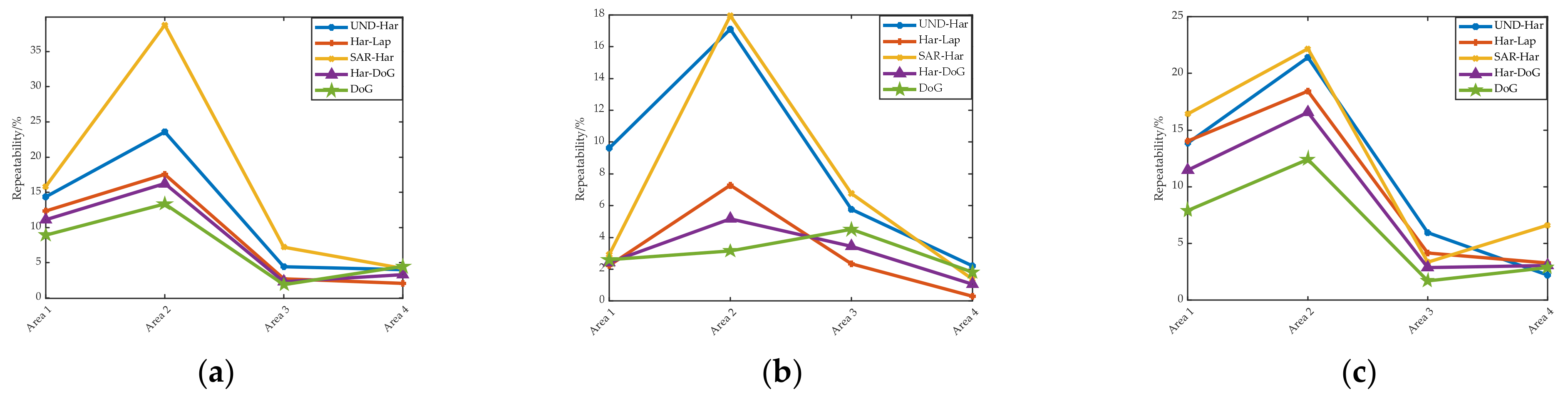
. GSD in Table 1 stands for ground truth spacing and there are no scale and rotation differences between each pair of images. All images are shown in Figure 9. The experimental results of the three sets of data are shown in Figure 10.

For each detector, we count the average of its repeatability across 12 image pairs obtained from four different regions and three different sensors as the final measurement indicator. The statistical results are shown in

Table 2. Average repeatability of five detectors.

Interest Point Detector	Average Repeatability/%
UND-Harris	10.375%
Har-Lap	7.2277%
SAR-Harris	11.9614%
Har-DoG	6.5823%
DoG	5.4669%

.

It can be seen from Table 2 that the average repeatability of SAR-Harris is the highest, followed by UND-Harris and Har-Lap. DoG is the lowest, and Har-DoG is between Har-Lap and DoG. From the results of the three sets of experimental data in Figure 10 alone, the five detectors have higher repeatability on area 2 and lower repeatability on area 3 and 4.

The three types of images in area 2 have prominent geometric structures and clear edge structures, which is conducive to the extraction of interest points. In area 3 and 4, there is a temporal difference between the images, and the texture information is weaker than the other three areas. It is not difficult to see that SAR-Harris has better repeatability than other operators on airborne SAR image and spaceborne SAR image data (SAR-Harris was proposed to solve the problem of heterogeneous SAR image matching), while in the other two sets of data It is comparable to the repeatability exhibited by UND-Harris. Since DoG detects Blob points, and speckle noise on SAR images can easily be mistakenly detected as Blob points, the repeatability of DoG is the lowest among the five detectors. The repeatability of Har-DoG in each pair of images is between Har-Lap and DoG, because Har-DoG is essentially a combination of the two.

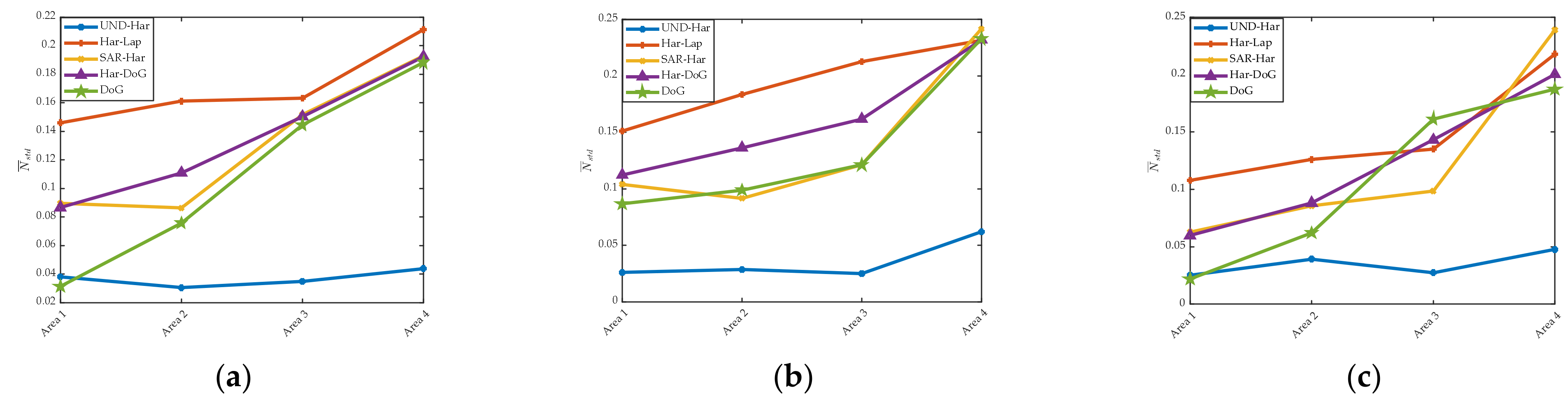
3.3. Distribution Uniformity

For image matching application, the uniformity of the location distribution of interest points on the image will affect the final image matching accuracy. Therefore, the interest point detector is required to detect relatively uniformly distributed interest points on both the reference image and the sensed image. This group of experiments uses three sets of image data in the nonlinear intensity difference adaptability experiment. For each sensor and different areas, the distribution uniformity N_std corresponding to the reference image and the sensed image are calculated, respectively. The average value of $N(—)$_std from two images is used as the final distribution uniformity indicator on this image pair. 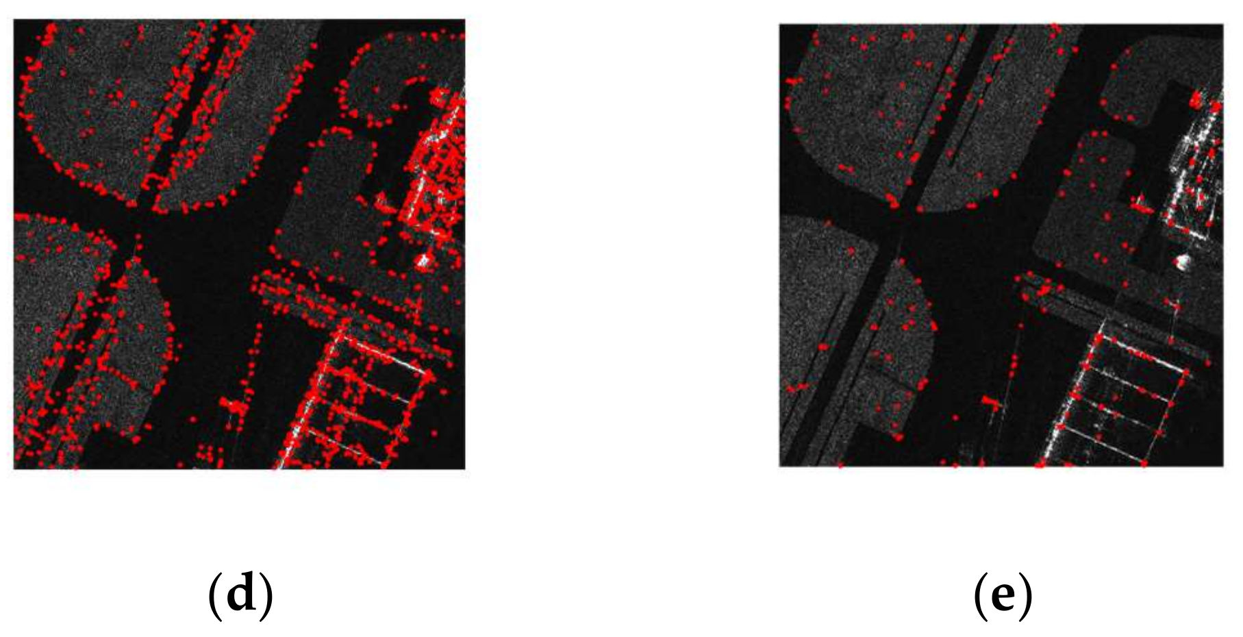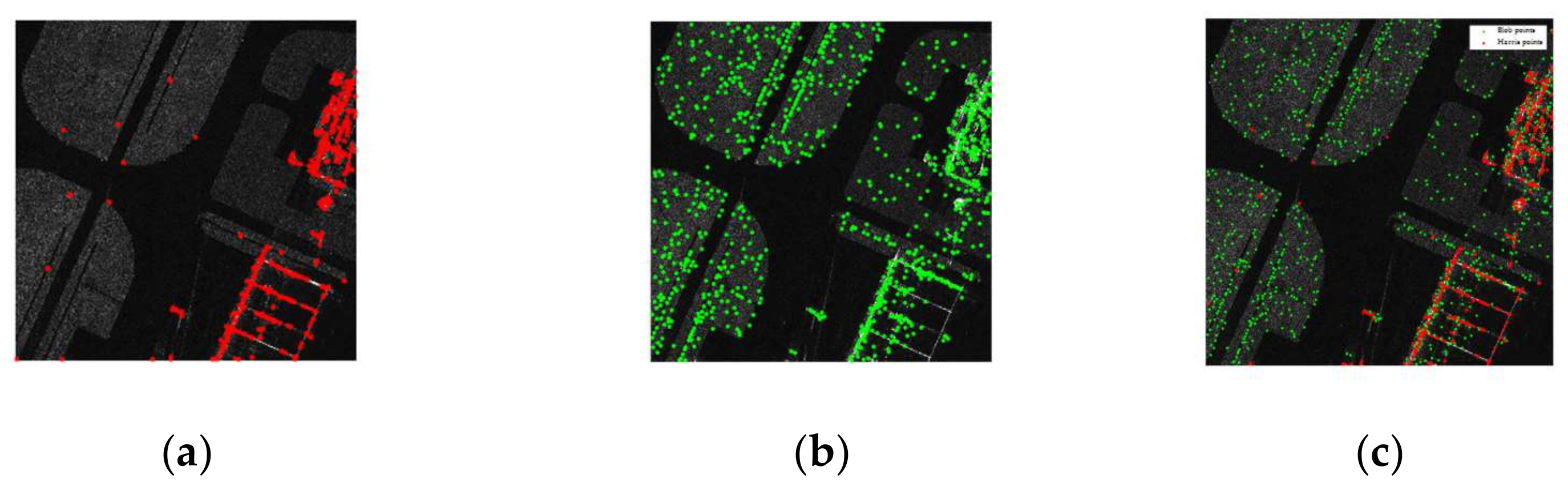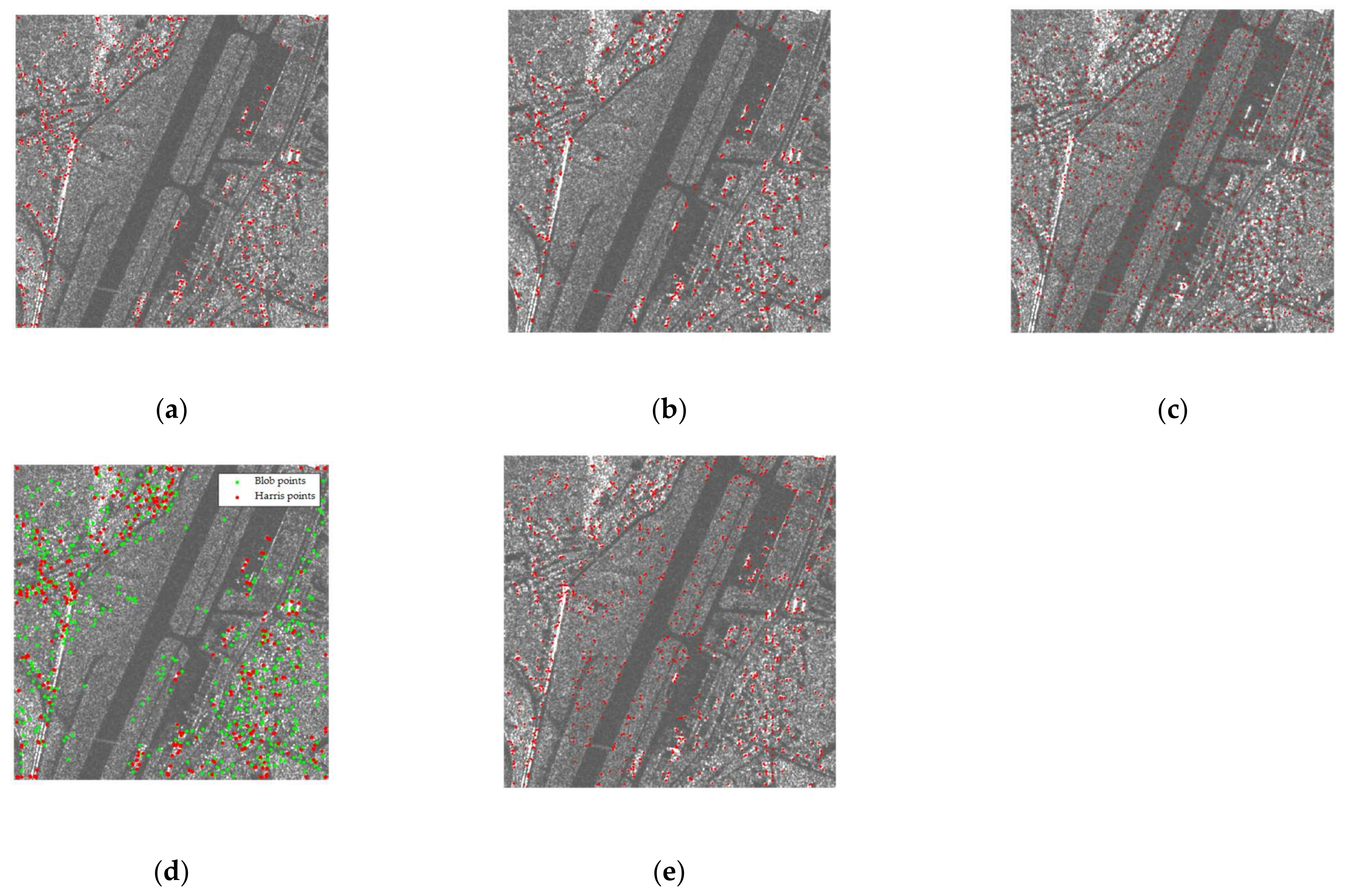The experimental results of three sets of data are shown in Figure 11. Taking the spaceborne SAR image as an example, the detection results of the five detectors are shown in Figure 12.

In general, it is not difficult to see that UND-Harris has the best distribution uniformity, followed by DOG and SAR-Harris, and the worst is Har-Lap. Har-DoG is between Har-Lap and DoG.

As mentioned in scale differences adaptability, although UND-Harris performs poorly on scale differences, due to its use of block strategy and feature scale to constrain the spatial position of interest points, the distribution uniformity of interest points is obviously better than the other four detectors. Har-Lap and SAR-Harris achieve corner extraction by thresholding the response function, with the result that when they are applied to SAR images, corners are mostly concentrated in areas with strong scattering targets (corresponding to very bright areas on the image, as shown in Figure 12a,b). Therefore, the distribution uniformity of both is not good. Among them, SAR-Harris uses ROEWA to suppress speckle noise, so that it can detect some corners with obvious geometric structures but weaker intensity than speckle noise. Therefore, the distribution uniformity of SAR-Harris is better than Har-Lap.

Since speckle noise is distributed evenly on SAR images, it is easily mistaken by DoG as Blob points (as shown in Figure 12c). The distribution uniformity of DoG is second only to UND-Harris in Figure 11a,c containing spaceborne SAR images (the signal-to-noise ratio of spaceborne SAR image is lower than that of airborne SAR image). Since Har-DoG integrates DoG and Har-Lap, its distribution uniformity is also between two detectors.

3.4. Image Alignment Performance Evaluation

Based on the experiments in Section 3.2, we use five different detectors for the image data in Table 1, and combine feature descriptor for image registration to further display the mosaic map. 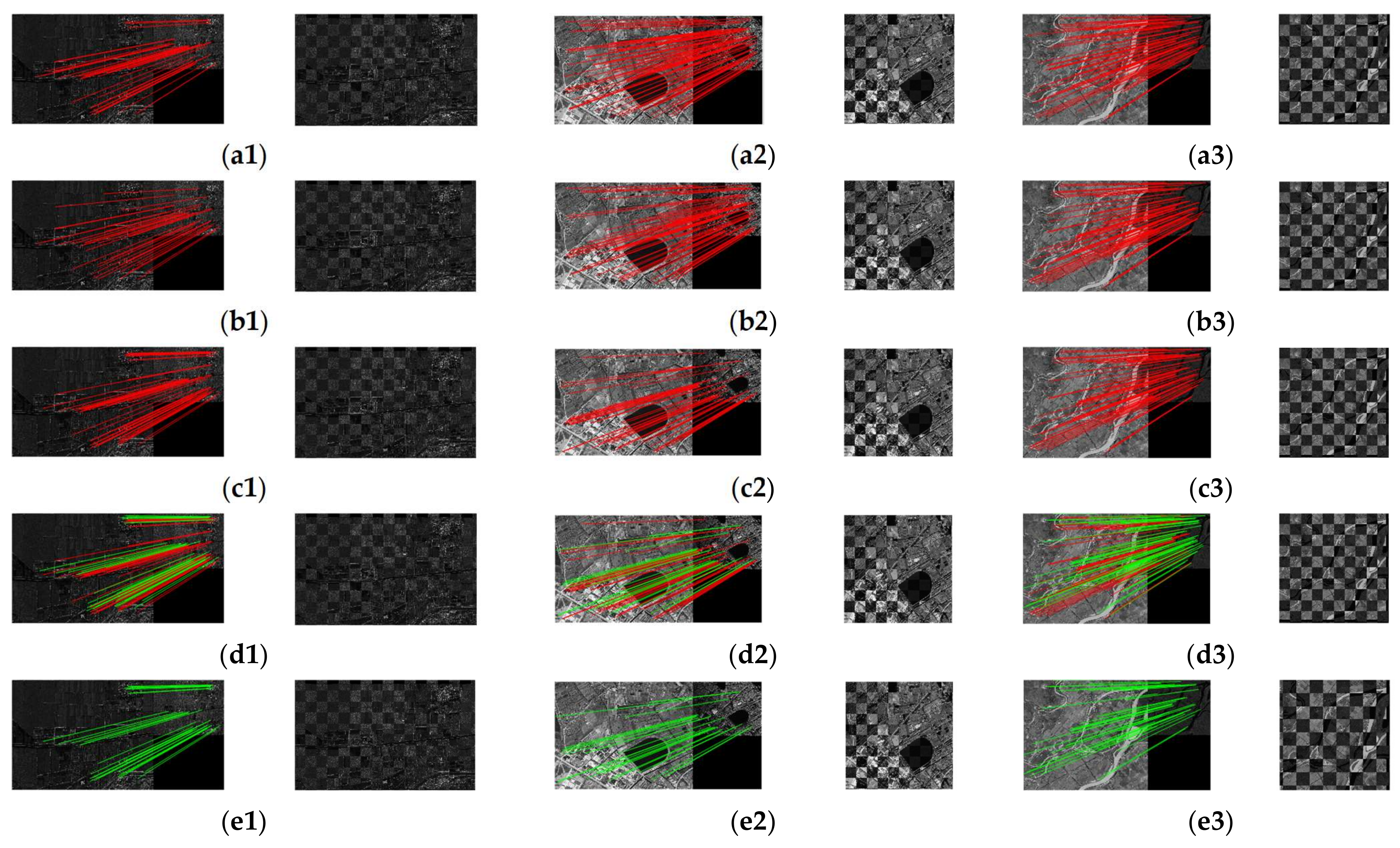Since the SIFT feature descriptor has poor performance when applied to heterogenous images, and the phase consistency (PC) is more robust to non-linear intensity differences between images, here we adopt the PCSD feature descriptor in [23] for feature description. Limited to the length of the article, we select a pair of images from the three sets of spaceborne SAR-to-airborne SAR, optical–to-airborne SAR and optical-to-spaceborne SAR data, respectively. The mosaic map is displayed after the final registration is completed. The results of the experiment are shown in Figure 13.

We scored the five detectors according to the alignment effect of the area marked by the red circle in the figure, and the obtained results are shown in

Table 3. Image Alignment Performance Score.

Interest Point Detector	Spaceborne SAR-to-Airborne SAR	Optical-to-Airborne SAR	Optical-to-Spaceborne SAR
SAR-Harris	★★★★★	★★★★☆	★★★★★
UND-Harris	★★★★☆	★★★★☆	★★★★☆
Har-DoG	★★★☆☆	★★★☆☆	★★★☆☆
Har-Lap	★★☆☆☆	★★☆☆☆	★★☆☆☆
DoG	★☆☆☆☆	★☆☆☆☆	★☆☆☆☆

“★” only represents the qualitative relationship, and does not quantitatively describe the performance of the detector.

below.

In Figure 13, the misalignment at the image junction corresponding to the mosaic image from the far left to the far right is increasing, which indicates that the quality of image alignment is deteriorating. As can be seen from Table 3, among the three types of image matching, SAR-Harris and UND-Harris are better aligned. Among them, SAR-Harris is comparable to UND-Harris in Optical-to-Airborne SAR data, and both types of images are better than the latter. Unexpectedly, Har-DoG, after being compared with the experimental results in Section 3.2, is finally better than the other two in image alignment quality, although Har-DoG is lower than Har-Lap and DoG in repeatability.

In the image alignment performance evaluation experiments, except for Har-DoG, the rest of the detectors’ performance rankings are consistent with the experimental results in Section 3.2. Because blob points are seriously disturbed by speckle noise in SAR images, its repeatability is lower than that of corner point, and the repeatability of Har-DoG combining the two is inevitably lower than that of Har-Lap. However, for the image matching application, the addition of blob point detection introduces more information to some extent (although it will further reduce the computational efficiency). Therefore, the performance comparison of interest point detectors cannot be based on repeatability alone.

3.5. Detection Efficiency

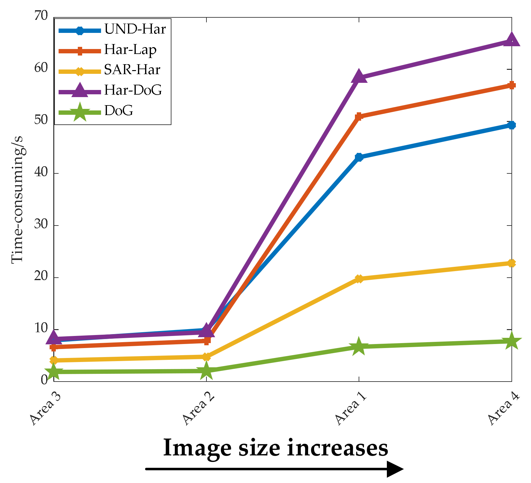
In this section, we study the feature detection efficiency of five detectors, select the airborne SAR and optical image sequences in Table 1, and manually adjust the detection threshold of each detector to control the detection of 1000 interest points on the reference image and the sensed image. The time consumption of each detector is shown in Figure 14.

As can be seen from the figure, as the image size increases, the differences in time-consuming of the five detectors are also greater. The detection efficiency of DoG is the highest, followed by SAR-Harris, and Har-DoG is the lowest. When the image size is small, Har-Lap outperforms UND-Harris, but when the image size is large, the two are opposite.

Although DoG performs poorly in adaptability to nonlinear intensity difference, it is significantly better than the other four operators in terms of detection efficiency. All five detectors need to establish a scale space. Since DoG down-samples the image when constructing the scale space and uses DoG instead of LoG when performing scale space localization, its detection time is shorter than other detectors. Although SAR-Harris is similar to Har-Lap, it needs to construct a SAR-Harris scale space, but it has obtained the scale attribute of interest points while completing the extreme value detection, so its detection efficiency is better than that of Har-Lap. Because the number of layers in the scale space constructed by Har-Lap is positively correlated with the image size, the detection efficiency of Har-Lap shows different pros and cons compared to UND-Harris when the image sizes are different. Har-DoG needs to detect corner points and Blob points at the same time, so its feature detection time takes the longest and has the lowest efficiency.

3.6. Comprehensive Evaluation

In order to more intuitively reflect the performance of the five detectors in above experiments, the performance evaluation table shown in

Table 4. Comprehensive performance evaluation of five detectors.

Interest Point Detector	Scale Difference Adaptability	Nonlinear Intensity Difference Adaptability	Distribution Uniformity	Detection Efficiency
SAR-Harris	★★★★★	★★★★★	★★★☆☆	★★★★☆
UND-Harris	★☆☆☆☆	★★★★☆	★★★★★	★★★☆☆
Har-Lap	★★☆☆☆	★★★☆☆	★☆☆☆☆	★★☆☆☆
Har-DoG	★★★☆☆	★★☆☆☆	★★☆☆☆	★☆☆☆☆
DoG	★★★★☆	★☆☆☆☆	★★★★☆	★★★★★

“★” only represents the qualitative relationship, and does not quantitatively describe the performance of the detector.

is made. As can be seen from the table, SAR-Harris shows the best repeatability under scale changes and nonlinear intensity difference between images. Although it was originally proposed to solve the multiplicative speckle noise in SAR image matching, it can still show good performance when applied to optical image and SAR image matching. This can also be derived from the score of image alignment performance. UND-Harris is proposed for matching optical images and SAR images. Although its repeatability is comparable to SAR-Harris on images with nonlinear intensity difference, the detector is sensitive to scale changes. The distribution uniformity of the interest points detected by UND-Harris is the highest among the five detectors, so when there is a large geometric distortion in the heterologous image, this detector is used to improve the final image matching quality.

Har-DoG combines Har-Lap and DoG to detect complementary corner points and blob points in an image, so it improves the density of interest points. Moreover, Har-DoG is better than Har-Lap and DoG in image alignment performance. However, the nonlinear intensity difference and speckle noise between optical image and SAR image are not fully considered in Har-DoG. Although DoG has poor adaptability to nonlinear intensity difference of heterologous images, it has high detection efficiency, good scale difference adaptability and distribution uniformity. Therefore, DoG is suitable for the coarse matching step in the two-stage matching strategy.

4. Discussion

Since the ground responses from different sensors and at different times are different, we show the performances of the co-registration of images with different scales and different sensors. In this section, we also combine PCSD feature descriptor and interest point detectors to register images and compare the impact of five different detectors on the final registration accuracy. The experiment uses images from different sensors, time and scales, and the image data information used is shown in

Table 5. Image registration experimental data.

Dataset Description
	Reference Image	Sensed Image	Image Characteristic
Test 1	Sensor: GF-3	Sensor: Airborne SAR	The imagery covers the suburban farmland, the overall texture information is weak, and there is strong speckle noise on the spaceborne SAR image. There is a 3× scale difference and a time difference of nearly two years between the two images.
	GSD: 1.5 m	GSD: 4.5 m
	Size: 2248 × 1391	Size: 983 × 856
	Date: November 2021	Date: 2020.03
Test 2	Sensor: Google Earth	Sensor: Airborne SAR	The imagery coverage area is relatively complex, including buildings, ponds, roads, etc., and the texture information is relatively rich. There is a 2× scale difference and a time difference of nearly two years between the two images.
	GSD: 1 m	GSD: 2 m
	Size: 1500 × 1500	Size: 731 × 769
	Date: May 2019	Date: 2021.04
Test 3	Sensor: Google Earth	Sensor: GF-3	The imagery coverage area contains a large number of rivers, and there is a clear intensity inversion between the optical image and the SAR image. There is a 2× scale difference and a time difference of more than a year between the two images.
	GSD: 10 m	GSD: 20 m
	Size: 1000 × 1000	Size: 487 × 512
	Date: May 2020	Date: 2021.09

.

The registration results of the three pairs of images are shown in Figure 15 below. In order to quantitatively compare the final performance of the five detectors, we calculated the root-mean-square error (RMSE) and the number of correct matching points (NCM) of the registration, respectively. The results are shown in

Table 6. Registration accuracy of five detectors.

Interest Point Detector	Test 1		Test 2		Test 3
	NCM	RMSE	NCM	RMSE	NCM	RMSE
UND-Harris	20	2.0967	61	1.6798	48	1.7084
Har-Lap	21	2.5621	38	2.7128	27	2.8641
SAR-Harris	19	1.6854	47	1.7009	49	1.7451
Har-DoG	25	2.4073	40	2.5188	33	2.7826
DoG	12	3.3828	23	2.9839	18	3.3743

.

In Figure 15, it can be seen that all detectors can finally complete the image regis-tration, and the matching points detected by UND-Harris and DoG are more uniform. As can be seen from Table 6, the RMSE of both UND-Harris and SAR-Harris is better than the other three detectors on the three pairs of images. Furthermore, in test 1, the RMSE of SAR-Harris is better than that of UND-Harris, while in test 2 and test 3, the accuracy of the two is comparable. Among the latter three detectors, Har-DoG has the highest accuracy and DoG has the lowest accuracy. It can be seen that the NCM of Har-DoG is larger than the other two.

From the final registration experimental results, compared with the previous experiments, the experimental results are consistent with the experimental results in 3.5. For Har-DoG, although its repeatability is between Har-Lap and DoG, both RMSE and NCM are better than the other two in registration experiments. This further shows that using both corner points and blob points for detection can indeed improve the registration accuracy of the final image and the density of matching point pairs. Comprehensive registration experiments further demonstrate that repeatability alone is not comprehensive enough as a criterion for evaluating detector performance.

5. Conclusions

Interest points, as key features on images, have been widely used in image matching. In order to select the most suitable interest point detector for specific applications, this paper starts from the application requirements of heterogeneous image matching, and integrates fives factors (scale difference adaptability, nonlinear intensity difference adaptability, interest point distribution uniformity, image registration alignment performance and detection efficiency), to evaluate the performance of five detectors: Har-Lap, DoG, Har-DoG, SAR-Harris, and UND-Harris. Experimental results show that the performance of interest point detectors varies for different evaluation aspects. In terms of scale difference and nonlinear intensity difference adaptability, SAR-Harris outperforms other detectors, among which DoG is second in scale difference adaptability, and UND-Harris is the weakest. UND-Harris is second only to SAR-Harris in adaptability to nonlinear intensity differences. In terms of distribution uniformity, UND-Harris showed the best performance, followed by DoG and SAR-Harris, and Har-Lap was the weakest. In terms of feature detection efficiency, DoG is the highest, followed by SAR-Harris. Har-DoG has the lowest efficiency due to the detection of two types of interest points. In terms of image alignment performance, Har-DoG is better than Har-Lap and DoG. In the other three aspects, the performance of Har-DoG is between Har-Lap and DoG. Regarding the image alignment performance as well as the final comprehensive registration results, only Har-DoG showed different results than adopting the repeatability metric. Therefore, SAR-Harris is optimal considering the five aspects of scale difference adaptability, nonlinear intensity difference adaptability, distribution uniformity, image registration alignment performance and detection efficiency. Although UND-Harris is weaker than SAR-Harris in detection efficiency and scale difference adaptability, its uniformity of interest point distribution makes it suitable for heterogeneous images with large local geometric distortion. In addition, when the sensed image contains a large number of textureless areas (such as water surfaces), the effect of using UND-Harris is not as good as SAR-Harris (UND-Harris will extract a large number of unreliable interest points in these areas of the image). Therefore, SAR-Harris is suitable for images with fewer effective texture areas, while UND-Harris is suitable for images with many effective texture areas. The excellent detection efficiency of DoG makes it more suitable for the coarse matching process in the two-stage matching method. Har-DoG is suitable for complementary detection when there are few corner points or blob points in the image to improve the density of interest points.

Choosing an optimal detector to carry out one’s own research cannot just rely on a single criterion. It is difficult to use a quantitative index to evaluate all detectors. Therefore, in actual research, we need to combine several evaluation indexes to select detectors according to our actual research needs. This paper also provides a reference for the selection of interest point detectors in the process of heterologous image matching.

References

1. Zitová, B.; Flusser, J. Image Registration Methods: A Survey. Image Vis. Comput. 2003, 21, 977–1000. [Google Scholar] [CrossRef] [Green Version]
2. Ye, Y.; Shan, J. A local descriptor based registration method for multispectral remote sensing images with non-linear intensity differences. ISPRS J. Photogramm. Remote Sens. 2014, 90, 83–95. [Google Scholar] [CrossRef]
3. Zukal, M.; Cika, P.; Burget, R. Evaluation of interest point detectors for scenes with changing lightening conditions. In Proceedings of the 2011 34th International Conference on Telecommunications and Signal Processing (TSP), Budapest, Hungary, 18–20 August 2011. [Google Scholar]
4. Cordes, K.; Rosenhahn, B.; Ostermann, J. Localization accuracy of interest point detectors with different scale space representations. In Proceedings of the 2014 11th IEEE International Conference on Advanced Video and Signal Based Surveillance (AVSS), Seoul, Korea, 26–29 August 2014. [Google Scholar]
5. Ehsan, S.; Kanwal, N.; Ostermann, J.; Clark, A.F.; McDonald-Maier, K.D. Measuring the Coverage of Interest Point Detectors. In Proceedings of the 8th International Conference on Image Analysis and Recognition (ICIAR)/International Conference on Autonomous and Intelligent Systems (AIS), Burnaby, BC, Canada, 22–24 June 2011. [Google Scholar]
6. Ruby, P.D.; Enrique, E.H.; Mariko, N.M.; Manuel, P.M.; Perez, G.S. Interest Points Image Detectors: Performance Evaluation. In Proceedings of the 2011 IEEE Electronics, Robotics and Automotive Mechanics Conference, Morelos, Mexico, 15–18 November 2011. [Google Scholar]
7. Barandiarán, I.; Graa, M.; Nieto, M. An empirical evaluation of interest point detectors. Cybern. Syst. 2013, 44, 98–117. [Google Scholar] [CrossRef]
8. Steffen, G.; Tobias, H.; Matthew, T. Evaluation of Interest Point Detectors and Feature Descriptors for Visual Tracking. Int. J. Comput. Vis. 2011, 94, 335–360. [Google Scholar] [CrossRef]
9. Gil, A.; Mozos, O.M.; Ballesta, M.; Oscar, R. A comparative evaluation of interest point detectors and local descriptors for visual SLAM. Mach. Vis. Appl. 2010, 21, 905–920. [Google Scholar] [CrossRef] [Green Version]
10. Pribyl, B.; Chalmers, A.; Zemci’k, P.; Hooberman, L.; Cadi’k, M. Evaluation of feature point detection in high dynamic range imagery. J. Vis. Commun. Image Represent. 2016, 38, 141–160. [Google Scholar] [CrossRef]
11. Melo, W.A.; Tavares, J.A.; Dantas, D.O.; Andrade, B.T. Improving Feature Point Detection in High Dynamic Range Images. In Proceedings of the 2018 IEEE Symposium on Computers and Communications (ISCC), Natal, Brazil, 25–28 June 2018. [Google Scholar]
12. Gunashekhar, P.K.; Gunturk, B.K. Improving the Performance of Interest Point Detectors with Contrast Stretching Functions. In Proceedings of the SPIE Conference on Image Processing: Machine Vision Applications, Burlingame, CA, USA, 6–9 March 2013. [Google Scholar]
13. Kazmi, W.; Andersen, H.J. A comparison of interest point and region detectors on structured, range and texture images. J. Vis. Commun. Image Represent. 2015, 32, 156–169. [Google Scholar] [CrossRef]
14. Molina, A.; Ramírez, T.; Díaz, G.M. Robustness of interest point detectors in near infrared, far infrared and visible spectral images. In Proceedings of the 2016 XXI Symposium on Signal Processing, Images and Artificial Vision (STSIVA), Bucaramanga, Colombia, 31 August–1 September 2018. [Google Scholar]
15. Wang, J.; Ye, Y.; Shen, L.; Li, Z.; Wu, S. Research on relationship between remote sensing image quality and performance of interest point detection. In Proceedings of the 2015 IEEE International Geoscience and Remote Sensing Symposium (IGARSS), Milan, Italy, 26–31 July 2015. [Google Scholar]
16. Ye, Y.; Shen, L. Performance Evaluation of Interest Point Detectors for Remote Sensing Image Matching. J. Southwest Jiaotong Univ. 2016, 51, 1170–1176. [Google Scholar] [CrossRef]
17. Schmid, C.; Mohr, R.; Bauckhage, C. Evaluation of Interest Point Detectors. Int. J. Comput. Vis. 2000, 37, 151–172. [Google Scholar] [CrossRef] [Green Version]
18. Mikolajczyk, K.; Schmid, C. Scale & affine invariant interest point detectors. Int. J. Comput. Vis. 2004, 60, 63–86. [Google Scholar] [CrossRef]
19. Lindeberg, T. Feature detection with automatic scale selection. Int. J. Comput. Vis. 1998, 30, 79–116. [Google Scholar] [CrossRef]
20. Lowe, D.G. Distinctive image features from scale-invariant keypoints. Int. J. Comput. Vis. 2004, 60, 91–110. [Google Scholar] [CrossRef]
21. Ye, Y.; Wang, M.; Hao, S.; Zhu, Q. A novel keypoint detector combining corners and blobs for remote sensing image registration. IEEE Geosci. Remote Sens. Lett. 2020, 18, 451–455. [Google Scholar] [CrossRef]
22. Dellinger, F.; Delon, J.; Gousseau, Y. SAR-SIFT: A SIFT-like algorithm for SAR images. IEEE Trans. Geosci. Remote Sens. 2014, 53, 453–466. [Google Scholar] [CrossRef] [Green Version]
23. Fan, J.; Wu, Y.; Li, M. SAR and optical image registration using nonlinear diffusion and phase congruency structural descriptor. IEEE Trans. Geosci. Remote Sens. 2018, 56, 5368–5379. [Google Scholar] [CrossRef]
24. Mikolajczyk, K.; Tuytelaars, T.; Schmid, C. A comparison of affine region detectors. Int. J. Comput. Vis. 2005, 65, 43–72. [Google Scholar] [CrossRef] [Green Version]
25. Aanæs, H.; Dahl, A.L.; Steenstrup, P.K. Interesting interest points. Int. J. Comput. Vis. 2012, 97, 18–35. [Google Scholar] [CrossRef]
26. Zhu, Q.; Wu, B.; Wan, N.; Steenstrup, P.K. An Interest Point Detect Method to Stereo Images with Good Repeatability and Information Content. Acta Electron. Sin. 2006, 34, 205–209. [Google Scholar] [CrossRef] [Green Version]
27. Zhu, H.; Zhao, C. Evaluation of the distribution uniformity of image feature points. J. Daqing Norm. Univ. 2010, 30, 9–12. [Google Scholar] [CrossRef]
Figure 1. Har-Lap detection process.
Remotesensing 14 03724 g001
Figure 2. Schematic diagram of interest points corresponding to five detectors: (a) Har-Lap. (b) DoG. (c) Har-DoG. (d) SAR-Harris. (e) UND-Harris.
Remotesensing 14 03724 g002aRemotesensing 14 03724 g002b
Figure 3. Schematic diagram of DoG scale space construction.
Remotesensing 14 03724 g003
Figure 4. Schematic diagram of extreme point detection of DoG detector.
Remotesensing 14 03724 g004
Figure 5. Results of nonlinear diffusion filtering and Gaussian filtering: (a) Gaussian filtering. (b) Nonlinear diffusion filtering.
Remotesensing 14 03724 g005
Figure 6. Schematic diagram of sub-region division: (a) Vertical direction. (b) Horizontal direction. (c) 45° direction. (d) 135° direction. (e) Center and periphery.
Remotesensing 14 03724 g006
Figure 7. SAR image with scale difference: (a) Airborne SAR reference image. (b) Airborne SAR 3× scale image. (c) Spaceborne SAR reference image. (d) Spaceborne SAR 3× scale image.
Remotesensing 14 03724 g007
Figure 8. The effect of scale difference on repeatability: (a) Airborne SAR images. (b) Spaceborne SAR images.
Remotesensing 14 03724 g008
Figure 9. Image pairs with nonlinear intensity difference: (a1a4) Airborne SAR images. (b1b4) Spaceborne SAR images. (c1c4) Optical images.
Remotesensing 14 03724 g009
Figure 10. Influence of nonlinear intensity difference on repeatability: (a) Spaceborne SAR-to-Airborne SAR. (b) Optical-to-Airborne SAR. (c) Optical-to-Spaceborne SAR.
Remotesensing 14 03724 g010
Figure 11. Distribution uniformity of interest points: (a) Spaceborne SAR-to-Airborne SAR. (b) Optical-to-Airborne SAR. (c) Optical-to-Spaceborne SAR.
Remotesensing 14 03724 g011
Figure 12. Detection results of five detectors on spaceborne SAR images: (a) Har-Lap. (b) SAR-Harris. (c) DoG. (d) Har-DoG. (e) UND-Harris.
Remotesensing 14 03724 g012
Figure 13. Mosaic map of registration results: (a1a3) SAR-Harris. (b1b3) UND-Harris. (c1c3) Har-DoG. (d1d3) Har-Lap. (e1e3) DoG. The red circle in the figure represents the stitching details of the image.
Remotesensing 14 03724 g013
Figure 14. Time-consuming of five detectors.
Remotesensing 14 03724 g014
Figure 15. Registration result and mosaic diagram: (a1a3) UND-Harris. (b1b3) SAR-Harris. (c1c3) Har-Lap. (d1d3) Har-DoG. (e1e3) DoG. Where the red lines denote the corners, and the green lines denote the blobs.
Remotesensing 14 03724 g015