Article

Inversion and Driving Force Analysis of Nutrient Concentrations in the Ecosystem of the Shenzhen-Hong Kong Bay Area

1
Institute of Space Science and Applied Technology, Harbin Institute of Technology at Shenzhen, Shenzhen 518055, China
2
Institute of Space Science, Shandong University at Weihai, Weihai 264209, China
*
Author to whom correspondence should be addressed.
Remote Sens. 2022, 14(15), 3694; https://doi.org/10.3390/rs14153694
Submission received: 19 June 2022 / Revised: 20 July 2022 / Accepted: 27 July 2022 / Published: 2 August 2022
(This article belongs to the Section Ocean Remote Sensing)

Abstract

:
Although satellite remote sensing technology is intensively used for the monitoring of water quality, the inversion of coastal water bodies and non-optically active parameters is still a challenging issue. Few ongoing studies use remote sensing technology to analyze the driving forces of changes in water quality from multiple aspects based on inversion results. By the use of Landsat 5/8 imagery and measured in situ data of the total nitrogen (TN) and total phosphorus (TP) in the Shenzhen-Hong Kong Bay area from 1986 to 2020, this study evaluated the modeling effects of four machine learning methods named Tree Embedding (TE), Support Vector Regression (SVR), Gaussian Process Regression (GPR), and Back-propagation Neural Network (BPNN). The results show that the BPNN creates the most reliable and robust results. The values of the obtained correlation coefficients (r) are 0.83, 0.92, 0.84, and 0.90, and that of the coefficients of determination (R2) are 0.70, 0.84, 0.70, and 0.81. The calculated mean absolute errors (MAEs) are 0.41, 0.16, 0.06, and 0.02, while the root mean square errors (RMSEs) are 0.78, 0.29, 0.12, and 0.03. The concentrations of TN and TP (CTN, CTP) in the Shenzhen Bay, the Starling Inlet, and the Tolo Harbor were relatively high, fluctuated from 1986 to 2010, and decreased significantly after 2010. The CTN and CTP in the Mirs Bay kept continuously at a low level. We found that urbanization and polluted river discharges were the main drivers of spatial and inter-annual differences of CTN and CTP. Temperature, precipitation, and wind are further factors that influenced the intra-annual changes of CTN and CTP in the Shenzhen Bay, whilethe expansion of oyster rafts and mangroves had little effect. Our research confirms that machine learning algorithms are well suited for the inversion of non-optical activity parameters of coastal water bodies, and also shows the potential of remote sensing for large-scale, long-term monitoring of water quality and the subsequent comprehensive analysis of the driving forces.

Graphical Abstract

1. Introduction

Water is an elemental natural resource necessary for functioning ecosystems and essential for human life. Globally, coastal areas have significantly higher population densities than non-coastal areas [1]. The ecosystems of coastal areas are relatively fragile, and any changes caused by human activities may endanger its stability. Therefore, the survival and development of human beings requires a continuous monitoring of existing water resources and their trophic state. It is estimated that 6 to 16 billion US dollars are lost [2] and more than 3 million people die [3] worldwide every year because of water pollution and eutrophication.
Traditional methods use on-site sample collection and laboratory analysis to ascertain the value of each water quality parameter. Main advantage is the accuracy, but the costs are also high and the procedure is time-consuming. Using the traditional point sampling method, it is difficult to realize the spatial and temporal changes of the water quality, as it is not conducive to the copious valuation and management of water bodies. Due to further limitations such as the topography, it may not be possible to monitor and manage larger water bodies [4]. In recent decades, with a rapid development of space science and computing power, remote sensing technology plays an increasingly important role in monitoring the quality of water bodies. It allows the synoptic assessment on a large-scale and over a long period efficiently and in a fast manner [5]. Different sensors operating from satellite and aircraft platforms measure the radiation of distinct wavelengths reflected or emitted from the top water volume. Based on various approaches, these signals are then used to retrieve the relevant water quality parameters.
The retrieval of water quality parameters by means of remote sensing techniques can be divided into empirical methods [6], semi-empirical methods [7], analytical methods [8], and semi-analytical methods [9]. The empirical and semi-empirical methods mainly involve statistical analyses, while the analytical and semi-analytic methods require a theoretical analysis of the spectral information [10]. Since the 1970s, with the availability of Landsat MSS, Landsat TM, Landsat ETM+, SPOT, MODIS, Sentinel-2, and further multi-spectral sensors, we see a continuously increasing number of scientific papers concerned with the assessment of water-quality parameters. Scholars pay more attention to optically active parameters such as chlorophyll-a (Chl-a), suspended particulate matter (SPM), colored dissolved organic matter (CDOM), and transparency (Secchi depth) than to non-optically active parameters such as total nitrogen (TN) and total phosphorus (TP). Estimating non-optically active parameters directly from spectral characteristics using a physical model is difficult, as they do not show distinct diagnostic spectral features measurable by multispectral satellite sensors [11,12]. There are relatively few inversion studies on remote sensing of non-optically active parameters [13]. However, these non-optically active water quality parameters are related to water eutrophication, and are important to environmental assessment and human health [14,15]. Fortunately, scientists found that non-optically active parameters are highly correlated with optically active parameters [16] and thus, can be estimated empirically and indirectly [17,18].
Previous studies confirmed that empirical models are feasible to retrieve the respective parameters when a statistical relationship between, e.g., TN and TP concentrations (CTN, CTP) and the respective reflectance values is established. Most of these models are based on linear, exponential, or logarithmic regressions [19,20,21], while machine learning algorithms excelled in improved performance [22,23,24]. Qiao et al. [25] and Jiang et al. [26] established the model of TN and TP in the Miyun Reservoir using twelve different machine learning algorithms. Niu et al. [14] developed and investigated two regression models based on deep learning to estimate seven optically inactive water quality parameters. However, the objects they studied were all inland water bodies. The coastal water body belongs to the so-called Case-II waters and is easily affected by tides and ocean currents, so its parameter inversion is more complicated.
With the establishment of the special economic zone in 1980, Shenzhen had developed rapidly, while the development of Hong Kong began after the World War II. They are closely connected, and the integrity and closeness of the ecosystem has formed the concept of the Shenzhen-Hong Kong ecosystem community. At present, there are only few studies focused on the boundary area between Shenzhen and Hong Kong, especially on the eastern sea area. Existing studies mostly concentrate on the Pearl River Estuary and Hong Kong, but there are few studies concerned with long time series and the assessment of non-optically active water parameters. Huang et al. [27] analyzed the changes of nutrients in the Shenzhen Bay on long time scales (more than 30 years) as one of the first. Wang et al. [28] found and confirmed the change law and trend of total suspended solid concentrations in the Pearl River Estuary. Nazeer et al. [29] evaluated empirical prediction models and neural network algorithms using the data of Landsat TM/ETM+ and HJ-1 A/B to estimate Chl-a and suspended solids concentrations in the coastal areas of Hong Kong.
Although previous studies have focused on the construction and application of water quality inversion models, they rarely combined multi-source data to further analyze the inversion results by remote sensing technology. Thus, our goal is not only to invert CTN and CTP, but to further analyze the driving factors for the changes from multiple perspectives.
Hence, this study aims at three essential issues. (1) Compare four machine learning methods (Tree Embedding, Support Vector Regression, Gaussian Process Regression, and Back-propagation Neural Network) and construct the most precise model for CTN and CTP at the border between Shenzhen and Hong Kong based on data of Landsat-5/8 and available monitoring stations. (2) Invert and compare the changes and their spatial variations over a long period of time (1986–2021). (3) Identify and analyze factors affecting water quality, including urbanization, river discharge, climate, oyster-farming, and mangrove forests.
In summary, this study provides a methodological reference to the inversion of non-optically active water quality parameters in coastal waters. It points out a comprehensive understanding of the issue in the study area at temporal and spatial scales, providing theoretical support for further improvement of the water quality and interregional cooperation. Finally, we demonstrate the potential of remote sensing methods for water quality monitoring and a comprehensive analysis of the driving forces.

2. Materials and Methods

2.1. Study Area

Shenzhen belongs to the Guangdong Province in China. It is adjacent to the Pearl River Estuary in the west and the Daya Bay and the Mirs Bay in the east. Hong Kong is located in the south of Shenzhen and adjacent to the South China Sea. The land area of Shenzhen and Hong Kong amounts to 1997 km2 and 1106 km2, the sea area to 1145 km2 and 1648.7 km2 respectively. The coastlines average to 260 km and 360 km, and the total population sums up to 13 million and 7.5 million respectively [30].
The boundary area between Shenzhen and Hong Kong chosen for the study, mainly includes the Shenzhen Bay, Mirs Bay, Starling Inlet, Tolo Harbor, and the Tolo Channel. The northern part of the Shenzhen Bay is connected with the Nanshan and Futian Districts of Shenzhen, and the southern part is connected to the Yuen Long District and the Tuen Mun District of Hong Kong. The northwest of the Dapeng Bay is the Yantian District of Shenzhen, the northeast and east are the Dapeng New Area of Shenzhen, and the west is the Northern District and the Sai Kung District of Hong Kong. The Tolo Harbor and the Tolo channel are surrounded by the Tai Po District of Hong Kong, connecting the Mirs Bay. For the analyses and the consecutive comparison of results, we established six monitoring areas (A–F) displayed in Figure 1 that also shows the map of the study area and the monitoring stations.

2.2. Data Sources

Measured water quality data from 1986 to 2020 are available from the Hong Kong Environmental Protection Department (HKEPD). The department has implemented a comprehensive seawater quality monitoring program since 1986 and conducts monitoring at 76 open water stations every month. Of these 76 monitoring stations, 22 are located within the study area and have been marked with red dots in Figure 1.
Satellite data used to build the CTN and CTP inversion models are recorded by Landsat-5 TM and Landsat-8 OLI sensors. The Landsat project was initiated by NASA and has the advantage of 50 years archived historical data. Landsat-5 TM data are available from 1984 to 2013 comprising seven bands with a ground sampling distance (GSD) of 30 m, providing three bands in the visible range, one band in the near-infrared, two bands covering the short-wave infrared, and one thermal band. The time range of used Landsat-8 OLI data reaches from 2013 to the present. Landsat-8 OLI has eight bands covering similar wavelength ranges as Landsat-5 TM, plus one band each for coastal applications and cirrus correction with 30 m GSD and one additional panchromatic band with 15 m GSD. The surface reflectance datasets of Landsat are available on the Google Earth Engine (GEE).
For the analysis of urbanization processes, we used the global impervious surface area (GISA) dataset created by Huang et al. [31]. In the climate analysis section, we used MOD11A1 version 006 data to obtain surface temperatures. Precipitation was achieved using data from the Climate Hazards Group InfraRed Precipitation with Station (CHIRPS) [32]. Information about the meridional and zonal components of wind based on a 10 m grid was derived from monthly averaged Reanalysis v5 (ERA5) data of the European Centre for Medium-Range Climate Forecasts (ECMWF) [33].

2.3. Method of Model Building

2.3.1. Preprocessing

The surface reflectance dataset of Landsat on GEE has already been preprocessed. So, we masked the clouds on the images and then extracted the spectral data of the sampling points. In order to maximize the number of combinations, we screened the spectral data according to the cloud coverage of the sampling points, rather than requiring the entire study area to be cloud-free. We then compared the acquisition dates of the spectral data with the measured data of TN and TP and extracted combinations where the spectral and the measured data did not differ more than three days per point. For the Landsat-5 TM sensor, six bands (Band 1–5 and 7) were extracted, and seven bands (Band 1–7) were selected for the Landsat-8 OLI sensor. This combination was then used for model building. To improve the modeling efficiency, the data were standardized, except when using the Tree Embedding method.
Before applying the model, the object was determined. When analyzing the inter-annual changes of CTN and CTP, the cloud-free images from October to December in 1986–2021 were selected to calculate the mean value by each year. If there were no images that meet the requirements, we decided for images in September of the same year or for January of the following year. This is because there are more cloud-free images in the study area from October to December, and the continuity of the results should be maintained as good as possible. When analyzing the inter-monthly changes, the cloud-free images from 2013 to 2021 were selected to calculate the mean per month.
Next, water extraction was performed. The modified normalized difference water index (MNDWI) [34], which uses the green and the SWIR I band for the enhancement of open water features, was calculated, and the Otsu method [35] was used for automatic threshold segmentation.

2.3.2. Tree Embedding (TE)

The classification and regression tree (CART) model was proposed by Breiman et al. [36]. For a given dataset x 1 , y 1 , x 2 , y 2 , , x m , y m , we recursively divide each region of the input space into two sub regions and decide the output value on each sub region.
First, select the splitting variable j and splitting point s at the following condition:
min j , s min c 1 x i R 1 ( j , s ) ( y i c 1 ) 2 + min c 2 x i R 2 ( j , s ) ( y i c 2 ) 2
where R 1 ( j , s ) = { x | x ( j ) s } and R 2 ( j , s ) = { x | x ( j ) > s } .
The division of space and output values are determined by the splitting variable and splitting point:
c ^ m = 1 N m x i R m ( j , s ) y i , m = 1 , 2
The above steps are repeated until the stop condition is satisfied. Then the decision tree is generated:
f ( x ) = m = 1 M c ^ m I , x R m
When dealing with specific practical problems, we can use the boosting and bagging methods in ensemble learning to improve and upgrade the regression tree [37].

2.3.3. Support Vector Regression (SVR)

The SVR regression tries to find a hyperplane in a high-dimensional space such that all the data in the set are closest to that plane [38]. An insensitive cost function (ε) was introduced by Vapnik [39] to form an ε-SV regression where we ignore errors as long as they are less than ε.
Suppose a given training dataset ( x 1 , y 1 ) , ( x 2 , y 2 ) , , ( x m , y m ) 𝒳 × , where 𝒳 denotes the space of the input patterns (e.g., 𝒳 = d ), then, for a given linear case, SVR is used to find a decision function:
f ( x ) = ω , x + b   with   ω 𝒳 , b
where , represents the dot product, ω is a normal vector of the hyperplane, and b is the bias parameter.
For a nonlinear case, we obtain a nonlinear SVR model using a nonlinear kernel function which can be introduced as [40]:
K ( x , x ) = ϕ ( x ) , ϕ ( x )
where ϕ ( x ) is a map from the sample space to the feature space. The kernel function makes non-linear separable cases linearly separable or approximate linear separability [41].

2.3.4. Gaussian Process Regression (GPR)

GPR is a probabilistic algorithm based on a nonparametric kernel [42]. If f ( x ) , x d is a Gaussian Process (GP), the joint distribution of the random variables f ( x 1 ) , f ( x 2 ) , f ( x n ) is also Gaussian. Using the independent likelihood and Bayes posterior inference, the joint posterior over f and f * could be given as:
p ( f , f * | y ) = p ( f , f * ) p ( y | f ) p ( y )
Since p ( y ) is a normalizing factor and the posterior p ( f , f * | y ) is Gaussian, we can assume that p ( f * | y ) shows also a Gaussian distribution [43]:
p ( f * | y ) N ( u * , σ * 2 )
u * = K f * , f ( K f , f + σ n 2 I ) 1 y
σ * 2 = K f * , f * K f * , f ( K f , f + σ n 2 I ) 1 K f , f *
where u * is the mean, σ * 2 is the variance, K is the covariance matrix, and I is the identity matrix.

2.3.5. Back-Propagation Neural Network (BPNN)

BPNN is an artificial neural network based on an error back-propagation algorithm [44]. It consists of three layers, namely the input layer, the hidden layer, and the output layer. Each layer contains at least one node which has a nonlinear activation function. Nodes are connected by links, each link represents a numerical weight. The modus operandi of the BPNN is divided into a feed forward of the input signals and a back propagation of the errors [45].
In the feed forward, the input layer receives external input information and passes it to the hidden layer. The task of the hidden layer is the processing of the internal information. The output layer accepts the processing result of the hidden layer and moves it to the output. The calculation formula can be found as:
x j l + 1 = f ( i w i j l x i l + w b j l + 1 )
E = 1 2 j ( x j l + 1 f ( x i ) ) 2
where x i l is the input at layer l , w i j l is the connection weight from neuron i at layer l to neuron j at layer l + 1 , w b j l + 1 is the bias of neuron j at layer l + 1 , and f ( ) is a nonlinear activation function. E is the output error and f ( x i ) is the actual output.
When the output error is unsatisfactory, back-propagation of the error is performed. Starting from the output layer, the error is back-propagated layer by layer to the hidden and input layers, and each weight is corrected according to the gradient descent of the error. Feedforward and backpropagation are repeated until the output error is reduced to an acceptable range or the predetermined learning time is reached.

2.3.6. Accuracy Assessment

Pearson’s linear correlation coefficient (r), the coefficient of determination (R2), the mean absolute error (MAE), and the root mean square error (RMSE) were used to evaluate the respective accuracy of the selected models. r shows the strength of the linear association between two variables. R2 is a measure of the proportion of the explained variance present in the data. The MAE is an arithmetic average of the absolute errors and reflects the magnitude of the actual prediction errors. The RMSE is the standard deviation of the prediction errors and measures how concentrated the data are around the line of best fit. Therefore, the closer the absolute values of r and R2 are to 1, and the smaller the values of the MAE and the RMSE, the higher the prediction accuracy of the model. They are defined as follows:
r = i = 1 N ( y ^ i y ^ ¯ ) ( y i y ¯ ) i = 1 N ( y ^ i y ^ ¯ ) 2 i = 1 N ( y i y ¯ ) 2
R 2 = i = 1 N ( y ^ i y ¯ ) 2 i = 1 N ( y i y ¯ ) 2
M A E = 1 N i = 1 N y ^ i y i
R M S E = 1 N i = 1 N ( y ^ i y i ) 2
where y i , y ¯ , y ^ i , y ^ ¯ are the measured, the mean measured, the estimated, and the mean estimated value, respectively; N is the number of samples.
To prevent overfitting and to improve model generalization, a five-fold cross validation is performed. For each cross validation, the entire data of the training set is randomly divided into 80% for training and 20% for validation. The RMSE of cross-validations are the average values of the validation sets [46].

2.3.7. Hyperparameter Optimization

There are generally two types of parameters in machine learning models. One needs to be learned and estimated from the data, called model parameters. Another type are the tuning parameters which need to be set manually in machine learning algorithms, called hyperparameters. Hyperparameters directly control the behavior and have a significant impact on the performance of machine learning models [47]. To determine the best combination of hyperparameters for the models, we used the Bayesian optimization procedure [48]. The optimal combination of hyperparameters minimizes the RMSE of cross-validations.
Bayesian optimization first generates an initial set of candidate points, and then calculates the mean and variance of the function value at each point according to the Gaussian process regression. The acquisition function is constructed from the mean and variance to represent the probability that it may be the optimal point. Sampling is performed at the position where the acquisition function is maximal, and then this point is also added to the set of candidate points. The above steps are repeated until the iteration is terminated. Finally, the point with the smallest value is selected as the solution to the problem. It is more efficient than grid search and random search because the information of previously searched points is used.

3. Results

3.1. Comparison of the Methods Accuracy

Combining the data of 22 water quality monitoring stations, we obtained 1553 combinations of Landsat-5 and TN, 411 combinations of Landsat-8 and TN, 1237 combinations of Landsat-5 and TP, 416 combinations of Landsat-8 and TP. Further, 80% of the data were selected as training sets and 20% were selected as test sets. The inversion models of TP and TN were established for the Landsat-5 and Landsat-8 data, named ‘TN-L5’, ‘TN-L8’, ‘TP-L5’, and ‘TP-L8’.
The best hyperparameter combinations found using an Bayesian optimization are shown in Table 1, and the corresponding RMSE of a five-fold cross-validation is shown in Table 2. When using the best hyperparameter combination, the RMSE obtained by the five-fold cross-validation of the training set is the smallest among the various hyperparameter combinations, thus, representing the best generalization ability. The best hyperparameter combinations were used to model the entire training sets, and the trained models were applied to the test sets. Thus, the r, R2, MAE and RMSE of the training sets, test sets, and all data sets were calculated and are depicted in Table 2.
(1) For the ‘TN-L5’ model, when using the TE and GPR, the r values of the training set are 1.00 for both, the R2 values are 0.99 and 1.00, the MAE values are 0.07 and 0.00, and the RMSE values are 0.10 and 0.00. There is an overfitting phenomenon, so these two methods are not selected. Comparing the results of the SVR and the BPNN, it can be seen that the BPNN performs better than the SVR for all indicators.
(2) For the ‘TN-L8’ model, the accuracy of each model on the test set is significantly different. The values of the r, R2, MAE, and RMSE of the BPNN reach 0.82, 0.67, 0.24, and 0.51, while that of the TE method amount to 0.57, 0.32, 0.33, and 0.71. The accuracy of the BPNN is also significantly higher when compared to the SVR and the GPR. On the training set, the accuracy of the BPNN is only marginally smaller than that of the GPR, with r values of 0.96 and 0.98, R2 values of 0.93 and 0.96, MAE values of 0.14 and 0.11, and RMSE values of 0.20 and 0.14. After modeling all data, the BPNN and the GPR show a comparable accuracy.
(3) For the ‘TP-L5’ model, when using GPR, the r value of the training set is 1.00, the R2 value is 1.00, the MAE is 0.00, and the RMSE is 0.00. There is a phenomenon of overfitting, so this method is not selected. On the training set, the r value of SVR is 0.61, the R2 value is 0.37, the MAE is 0.09, and the RMSE is 0.15, which is quite lower than that of the TE and BPNN, so this method is also not selected. On the test set, the accuracy of the BPNN method is better than that of TE, with r values of 0.77 and 0.71, R2 values of 0.60 and 0.51, MAE values of 0.08 and 0.09, and RMSE values of 0.17 and 0.19.
(4) Concerning the ‘TP-L8’ model on the test set, the BPNN produces the highest accuracy, slightly better than that of the SVR, with r values of 0.79 and 0.76, R2 values of 0.63 and 0.58, MAE values of 0.02 for both, and RMSE values of 0.04 for both. On the training set, the accuracy of the BPNN method is significantly better than that of the SVR method, with r values of 0.92 and 0.73, R2 values of 0.85 and 0.53, MAE values of 0.02 for both, and RMSE values of 0.03 and 0.05, respectively.
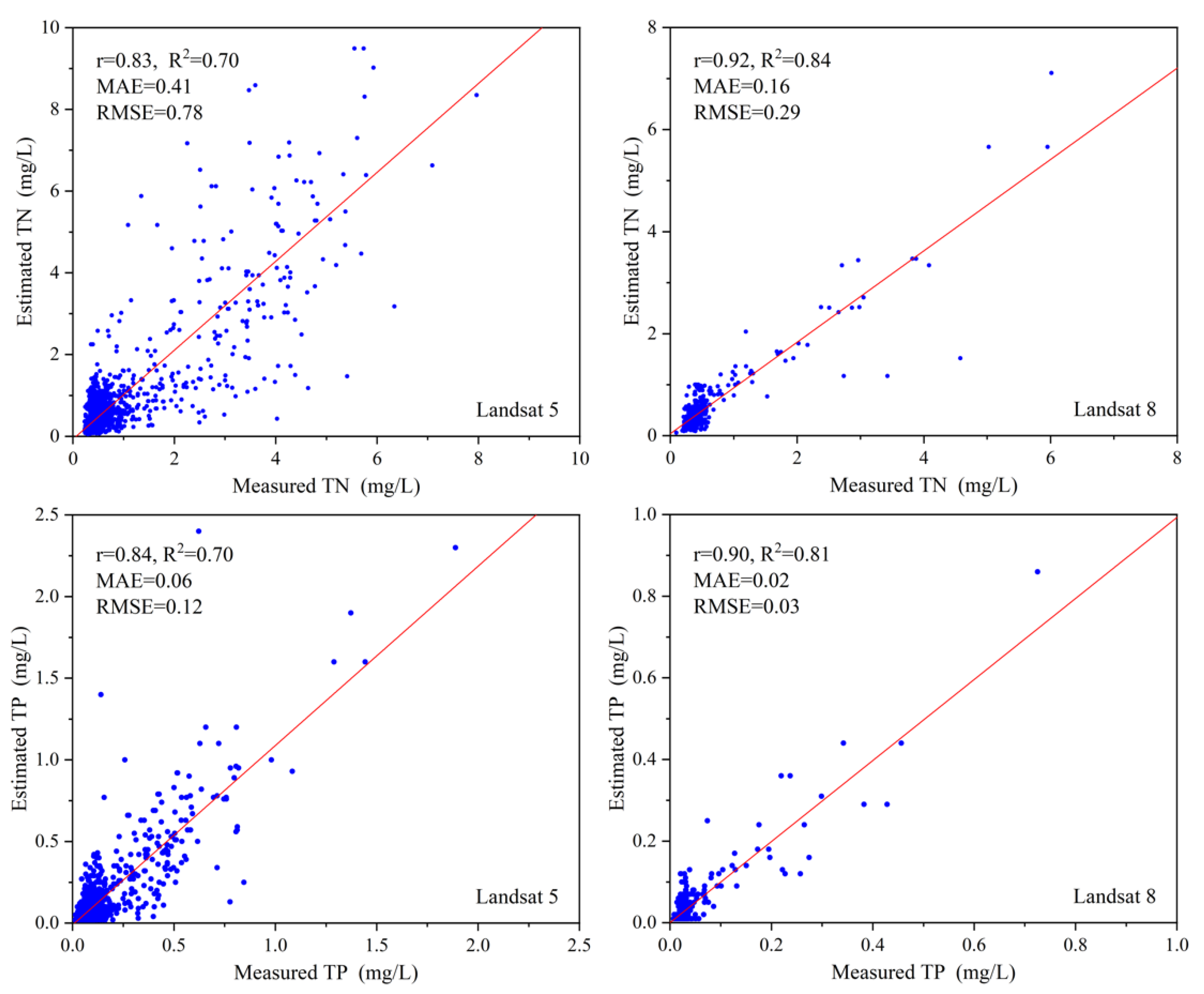
From all values determined above, the BPNN method is selected as the most suitable one for modeling. Hence, we performed the inversion of CTN and CTP using the models built by the BPNN. The modeling effect of the BPNN with all data is shown in Figure 2. It is indicated that there is a good fit between the measured and the estimated data for all four cases, and the inversion accuracy using Landsat 8 is higher than that when utilizing Landsat 5 data. For ‘TN-L5’, ‘TN-L8’, ‘TP-L5’, and ‘TP-L8’, the obtained r values are 0.83, 0.92, 0.84, and 0.90, the R2 values are 0.70, 0.84, 0.70, and 0.81, the MAE values are 0.41, 0.16, 0.06, and 0.02, the RMSE values are 0.78, 0.29, 0.12, and 0.03. The r and R2 values are relatively close to 1 while the values of the MAE and RMSE tend to be low. This indicates that the BPNN method is well suited for the construction of all four models.

3.2. Spatial Distribution

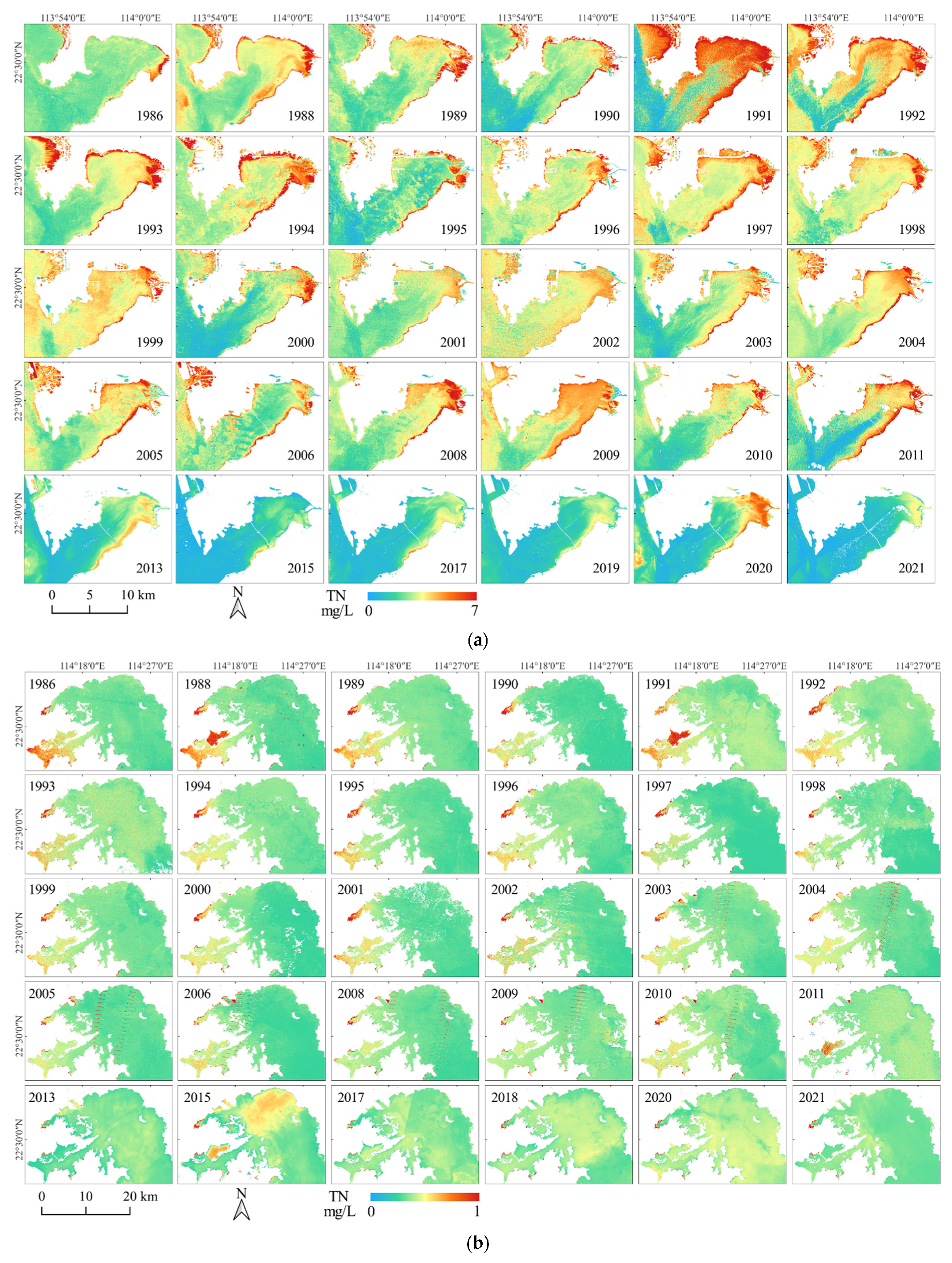
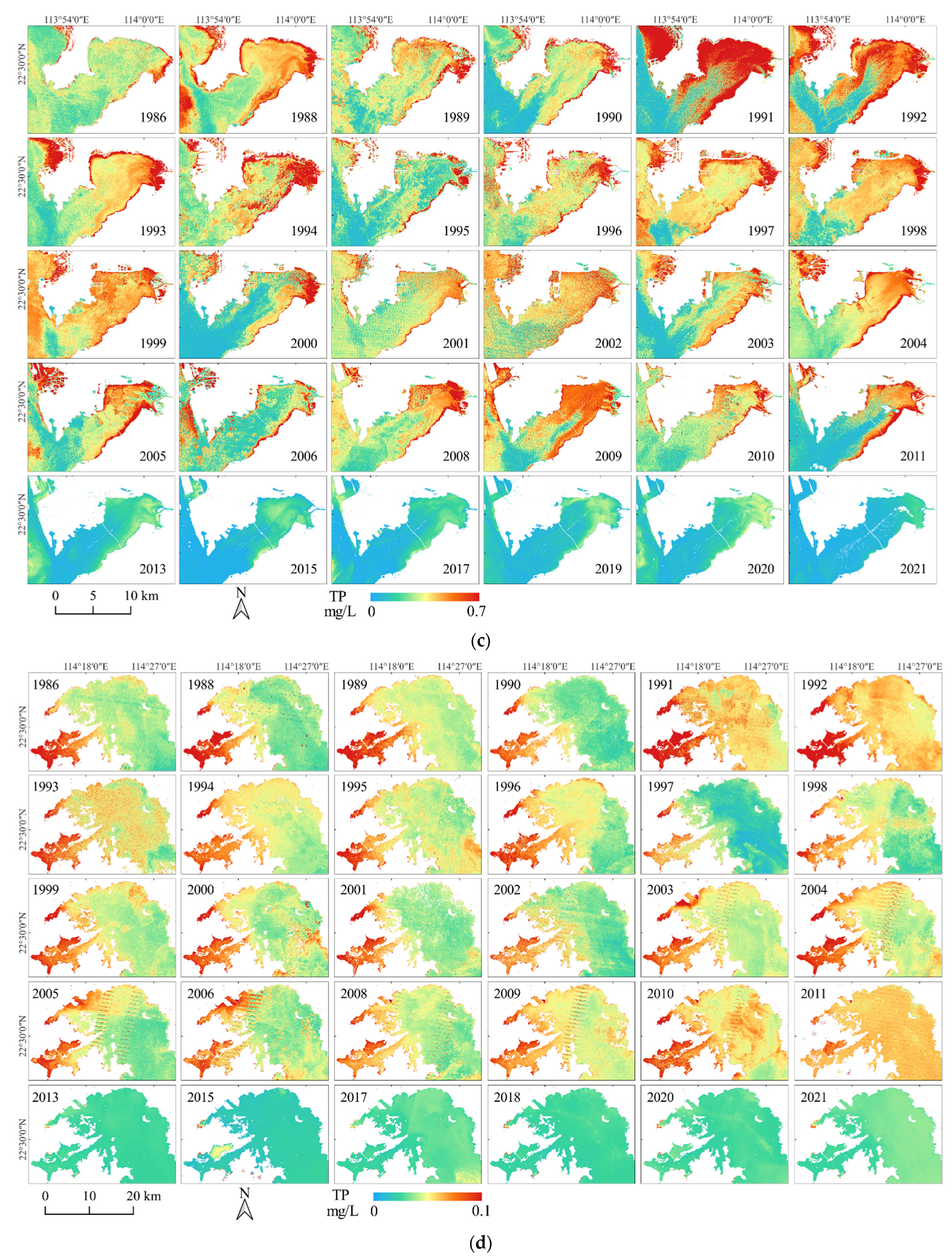
In terms of spatial differences, the situation is similar for TN and TP. Overall, the nutrient concentrations in the western part of the study area were significantly higher than those in the eastern part. The location of the six monitoring areas (A–F) can be seen in Figure 1. In the Shenzhen Bay, CTN and CTP decreased gradually from the inner bay (area A) to the outer bay (area B), and CTN and CTP on the southeast coast were generally higher than on the northwest coast (Figure 3a,c). In the western part of the study area, the nutrient concentrations in the Starling Inlet (area C) and the Tolo Harbor (area D) were higher than those in the inner bay (area E) and the outer bay (area F) of the Mirs Bay. Moreover, CTN and CTP gradually decreased from the Starling Inlet and the Tolo Harbor to the Mirs Bay, and also gradually decreased from the inner area to the outer area of the Mirs Bay, as shown in Figure 3b,d. The average CTN in areas A–F were 3.14, 2.02, 0.70, 0.51, 0.35, 0.33 mg/L and the average CTP were 0.35, 0.21, 0.10, 0.08, 0.04, and 0.04 mg/L.

3.3. Inter-Annual Changes

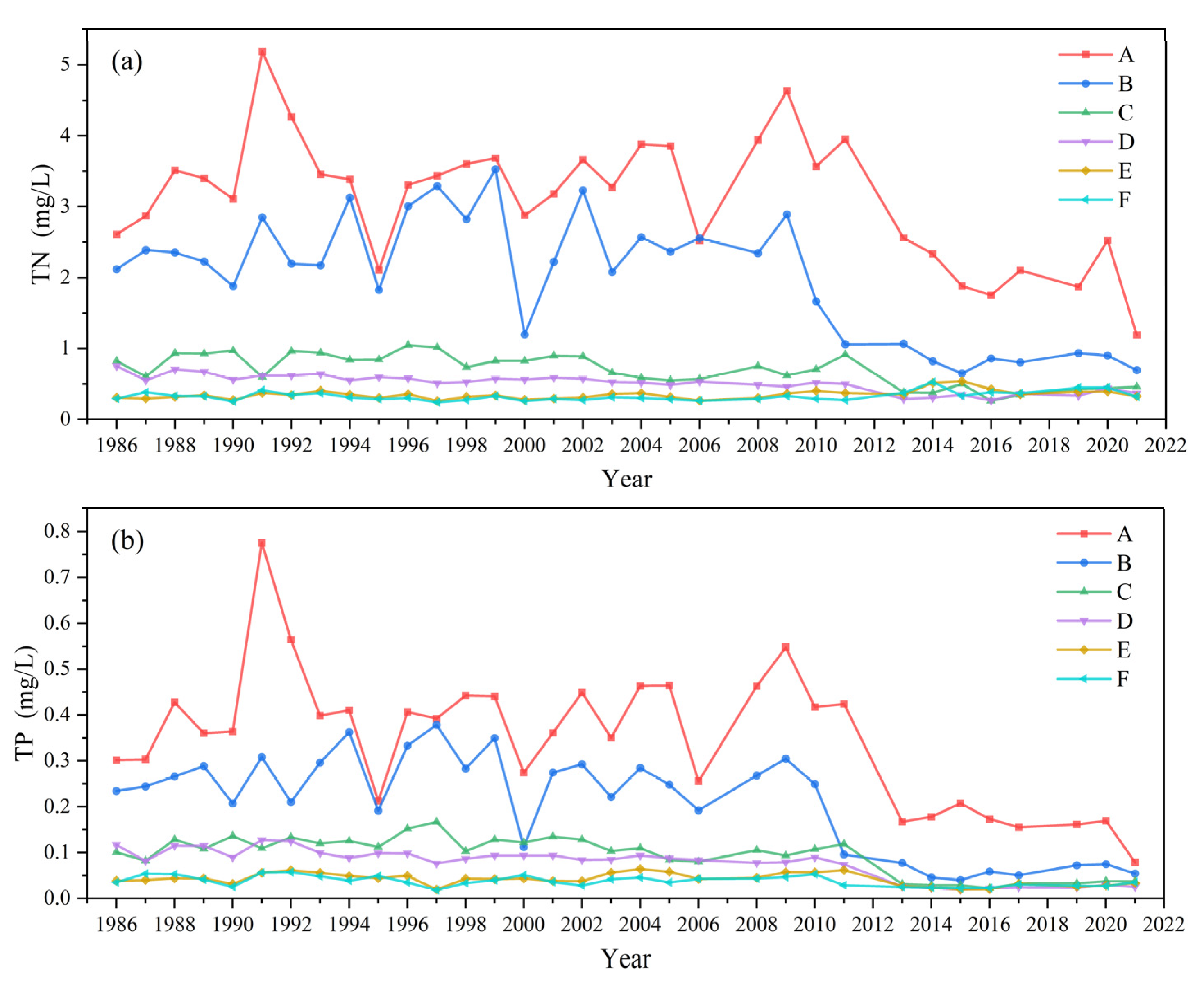
In terms of inter-annual differences, the changes in TN and TP were also similar. The CTN and CTP in areas A and B fluctuated from 1986 to 2010 and decreased significantly after 2010. The ranges of variation of CTN in areas A and B from 1986 to 2010 are 2.11–5.19 mg/L and 1.20–3.53 mg/L, and the ranges after 2010 are 1.19–3.95 mg/L, 0.65–1.07 mg/L respectively. CTP fluctuated in areas A and B from 1986 to 2010 at 0.21–0.78 mg/L, and 0.11–0.38 mg/L and after 2010 at 0.08–0.42 mg/L, and 0.04–0.10 mg/L respectively. The CTN and CTP in areas C and D also decreased after 2010, but this is not obvious because the CTN and CTP were lower than 1 mg/L and 0.2 mg/L before 2010. The CTN and CTP in areas E and F are the lowest, where TN is below 0.6 mg/L, and TP below 0.07 mg/L. Figure 4 shows the inter-annual differences of CTN and CTP.

3.4. Intra-Annual Changes

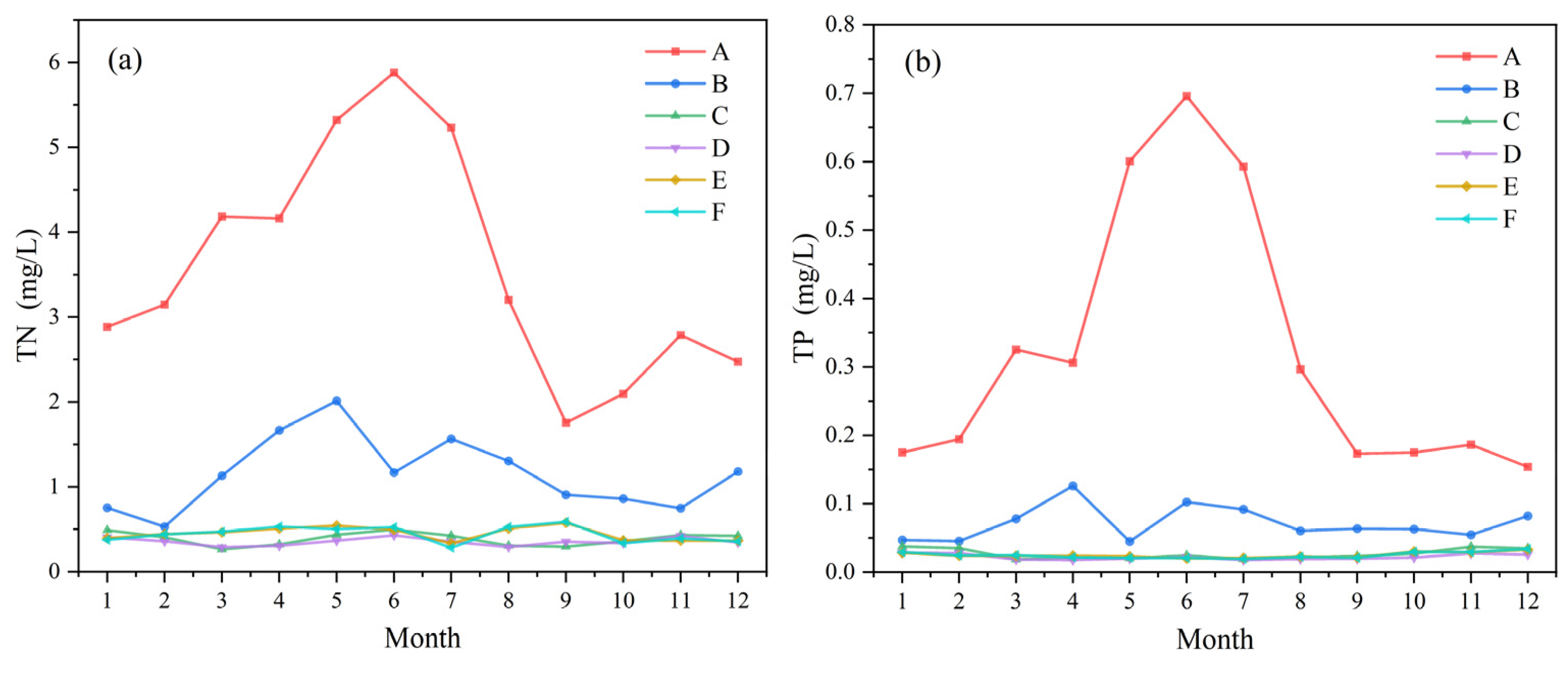
The intra-annual changes of CTN and CTP in the western part of the study area are obvious, while those in the eastern part are stable at low levels throughout the year, as shown in Figure 5. The intra-annual changes of CTN and CTP in area A are the most discernible ones among the six observed areas, peaking from May to July. The maximum values of CTN and CTP in area A appeared in June at 5.88 mg/L and 0.70 mg/L. The minimum values appeared in September and December at 1.76 mg/L and 0.15 mg/L. The maximum values are 3.35 and 4.52 times the minimum value. There are also visible intra-annual changes in area B. Similar to area A, CTN and CTP show small peaks from April to July. The maximum values of CTN and CTP in area B appear in May and April at 2.01 mg/L and 0.13 mg/L. The minimum values appear in February at 0.53 mg/L and 0.05 mg/L. The maximum values are 3.79 and 2.79 times the minimum value.

4. Discussion

4.1. Impact of Urbanization

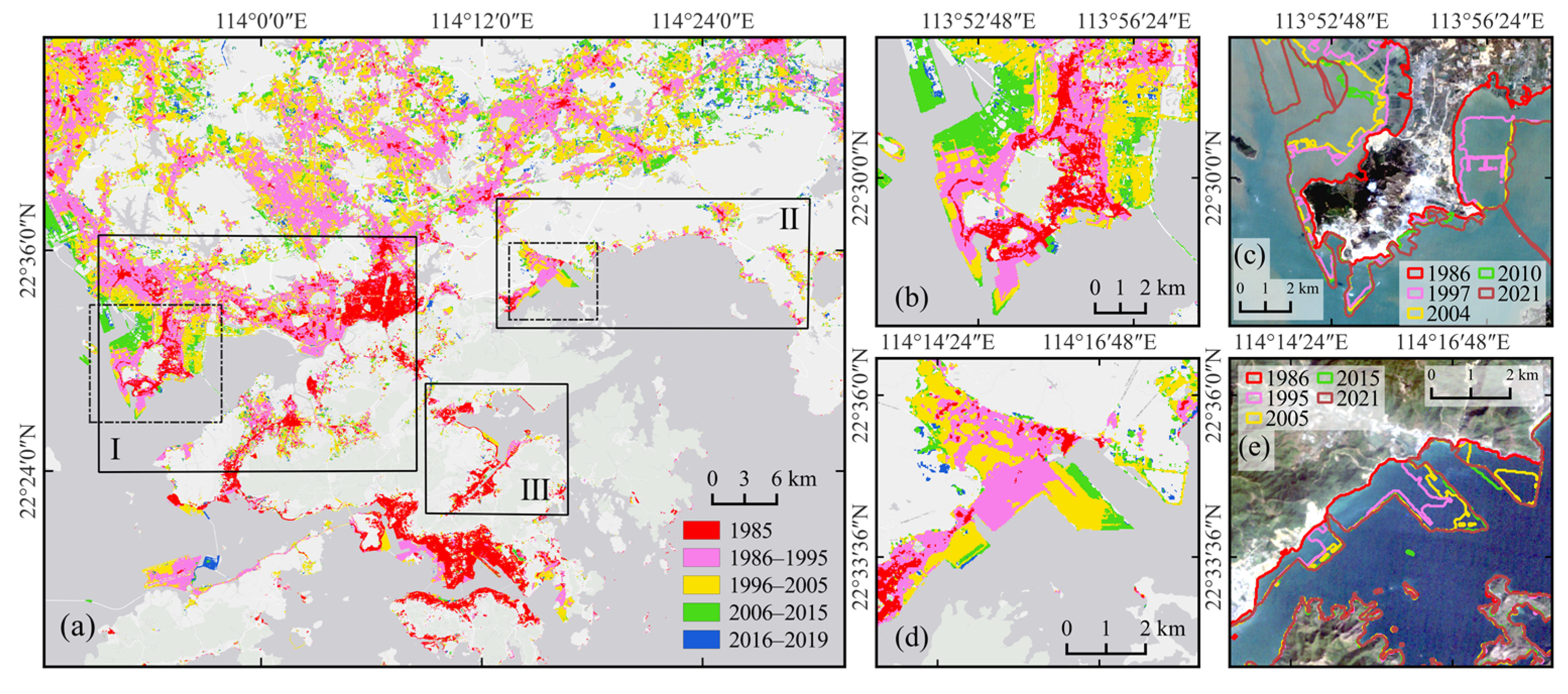
In context with the concentrations of TN and TP, we analyzed the urbanization process at a large scale through the temporal and spatial changes of the impervious surface areas (ISA) and depicted the respective land reclamation by the changes along the coastlines. The ISA is derived from the GISA dataset, and the coastlines are extracted from averaged images of Landsat-5 and Landsat-8 from October to December each year from 1986 to 2021 by the MNDWI and Otsu methods. Figure 6 shows the spatiotemporal changes of the ISA, the coastlines and the location of the monitoring areas (I, II, and III). Figure 7 displays the regional statistical results of the ISA in the respective areas.
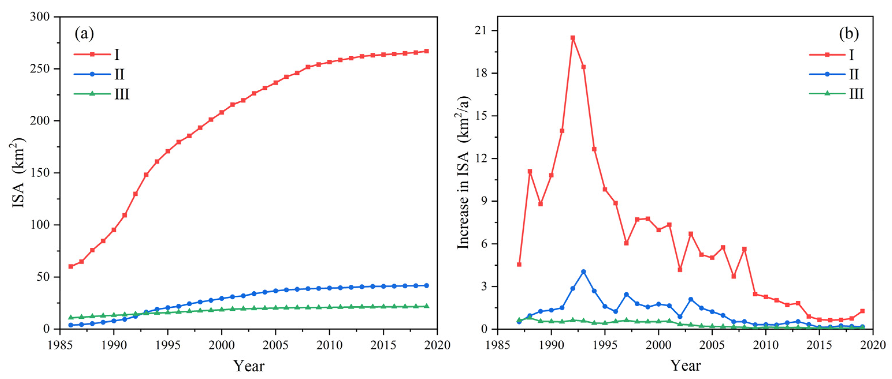
In terms of spatial distribution, the urbanization level in the western part of the study area was higher than that in the eastern part, and that in the northern part developed later than that in the southern part. In terms of inter-annual changes, the conversions in the ISA of areas I and II are similar, with a rapid increase at first, followed by a gradual decline in growth rate, while that in area III remained stable. Specifically, the ISA of area I accelerated in an expansion from 1987 to 1992, from 60.15 km2 to 129.85 km2, and the growth rate increased from 4.55 km2/a to 20.50 km2/a. In 1993–1997, the ISA increased from 148.30 km2 to 185.70 km2, but the growth rate dropped significantly, from 18.45 km2/a to 6.04 km2/a. In 1998–2010, the ISA increased from 193.41 km2 to 256.52 km2, and the growth rate fluctuated down, from 7.72 km2/a to 2.27 km2/a. In 2011–2019, the ISA increased from 258.56 km2 to 266.96 km2, and the growth rate was always lower than 2.04 km2/a in 2011. The trend change of the ISA in area II is similar to that in area I. The peak growth rate appeared in 1993, at 4.05 km2/a. After 2010, the growth rate was always lower than 0.55 km2/a. In 1986–2019, the ISA of area II increased from 3.79 km2 to 41.83 km2. The ISA of area III increased from 10.72 km2 to 21.66 km2 in 1986–2019, and the growth rate was always lower than 0.80 km2/a.
Considering Figure 3 and Figure 6 together, we found that the areas with high concentrations of TN and TP (the inner area of the Shenzhen Bay, Starling Inlet, and Tolo Harbor) are all close to or surrounded by urban areas. Examining Figure 4 and Figure 7 in combination, it is found that the urbanization processes in the study area tends to be slow in the past 10 years, corresponding to the maintenance of CTN and CTP at low levels. Several previous studies also confirmed the nonlinear relationship between impervious surface areas and water quality parameters [49,50]. The increasing construction activities regarding high-rise buildings and extensive reclamation projects in combination with human activities such as aquaculture, farming, and industrial activities all affect the quality of the water. Thus, the decline of urbanization has a corresponding positive effect on the water quality, as well as the fact that both cities, Shenzhen and Hong Kong, devote more attention to the matter.
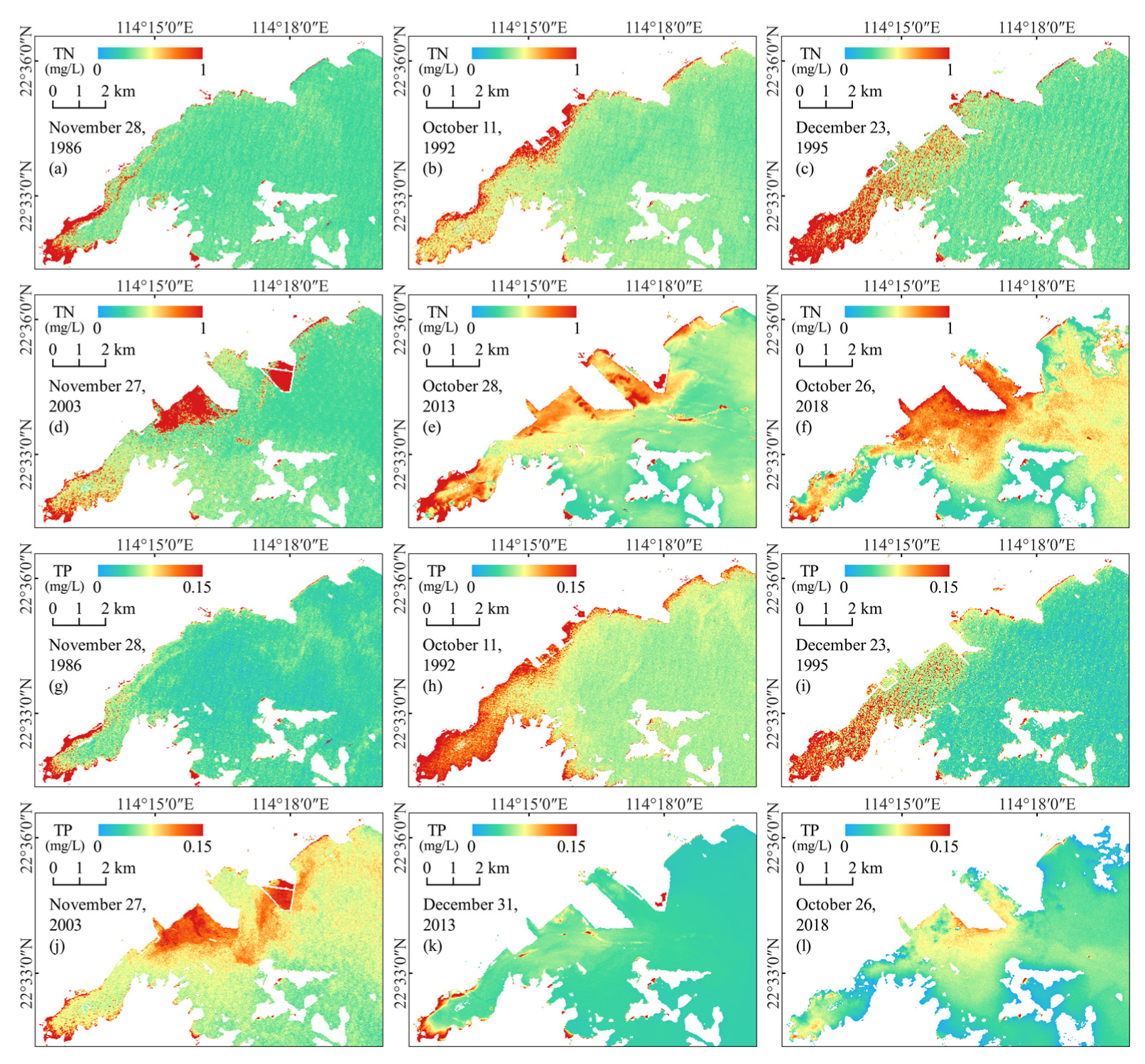
From Figure 6, it can be seen that both, the Shekou Peninsula and the Yantian Port show obvious coastal reclamations. However, the water quality around the Shekou Peninsula is greatly affected by further factors such as ocean currents in the Pearl River Estuary. Therefore, the Yantian Port is used as an example to analyze the impact of reclamation on water quality. The Yantian Port is located in the north of the Mirs Bay and is an important maritime transportation hub in South China. As of 2021, the port is dimensioned for 20 large deep-water berths with a quay length of 8212 m and a coastal water depth of 17.4 m [51]. All cloud-free Landsat-5 and Landsat-8 images of the Yantian Port from 1986 to 2021 were used for inversion of TN and TP. The representative results selected are displayed in Figure 8.
The construction of the Yantian Port led to significant changes in the spatial distribution of CTN and CTP. From Figure 8a,g, one can imagine that there was no significant difference between the seawater in the Yantian Port area and the surrounding area before the construction of the port. The process of port construction brought an abnormal increase in nutrient concentration along the coast (Figure 8b,h). Figure 8c,i shows the blocking of the high-concentration nutrients in the Starling Inlet when flowing into the Mirs Bay and accumulated in the west side of the Yantian Port. Figure 8d–f,j–l depict that the nutrient concentration around the port was significantly higher than in the surrounding sea. This has its cause in the accumulation of nutrient sources or pollutants through discharges from high-intensity port vessel activities, loading and unloading processes, and dredging [52]. It induces the eutrophication of water [53], what ultimately leads to algal blooms [54,55]. Especially in the second half of 2003, we observed abnormal occurrences of CTN and CTP around the Yantian Port on all images.

4.2. Impact of Rivers

The water quality of rivers is another important factor affecting coastal water quality. Pollutants generated by human activities flow into tributaries through surface runoff and underground pipelines, and then converge into the sea, causing direct pollution of coastal waters. Topographical obstacles also affect the assimilative capacity of pollutants [56]. The Shenzhen Bay is a semi-closed shallow bay with an average depth of only about three meters. The Tolo Harbor is surrounded by land and is connected to the Mirs Bay only by the narrow Tolo Channel.
A total of six rivers discharge directly into the Shenzhen Bay. Five of them have their catchment area in the Shenzhen area, namely the Shenzhen River, Fengtang River, Dasha River, Xiaosha River, and Houhai Central River while one, the Shanbei River, has its catchment in the Hong Kong area. Figure 3a,c clearly indicates the high CTN and CTP values in the Shenzhen Bay are concentrated in the northeast and in the estuaries of the Shenzhen River and Shanbei River. In 2000, Shenzhen and Hong Kong jointly formulated the Joint Implementation Plan for Water Pollution Prevention and Control in the Shenzhen Bay, which listed the pollution control measures to be taken at different stages, aiming to expand and improve the sewage treatment infrastructure to reduce the wastewater discharge [57]. From 2005 to 2009, Hong Kong reduced the nutrient pollution in the Shanbei River by voluntarily relinquishing poultry and pig production licenses [31]. During the “Twelfth Five-Year Plan” and “Thirteenth Five-Year Plan” period, Shenzhen’s sewage treatment system focused on rain and sewage diversion and sewage interception treatment was completed and put into operation. At the same time, Shenzhen has strengthened the comprehensive management of drainage, and managed 159 black and odorous water bodies and 1467 small and micro black and odorous water bodies [58].
The main rivers flowing into the Tolo Harbor are the Tai Po River, Lam Tsuen River, Tai Po Kau Stream, and Shing Mun River. The Plover Cove Reservoir was constructed in the 1970s, which cut off the stream that previously flowed directly into the Tolo Harbor, resulting in a significant reduction of drainage into the Tolo Harbor area. The urbanization and industrialization of Tai Po and Sha Tin have increased the burden on the Tolo Harbor ecosystem [59]. Hong Kong designated Tolo Harbor as Hong Kong’s first water control zone in 1982. The Tolo Harbor Action Plan (THAP) and the Tolo Harbor Effluent Export Scheme (THEES) were also implemented in 1987 and 1995 [60]. The government allowed to discharge treated sewage from the Sha Tin Sewage Treatment Works and the Tai Po Sewage Treatment Works through the Kai Tak River to the Victoria Harbor. Implementing sewage discharge control, banning livestock breeding, providing and improving sewage collection and treatment facilities, actively laying sewers for villages, and other measures were also used to improve water quality [61].

4.3. Impact of Climate

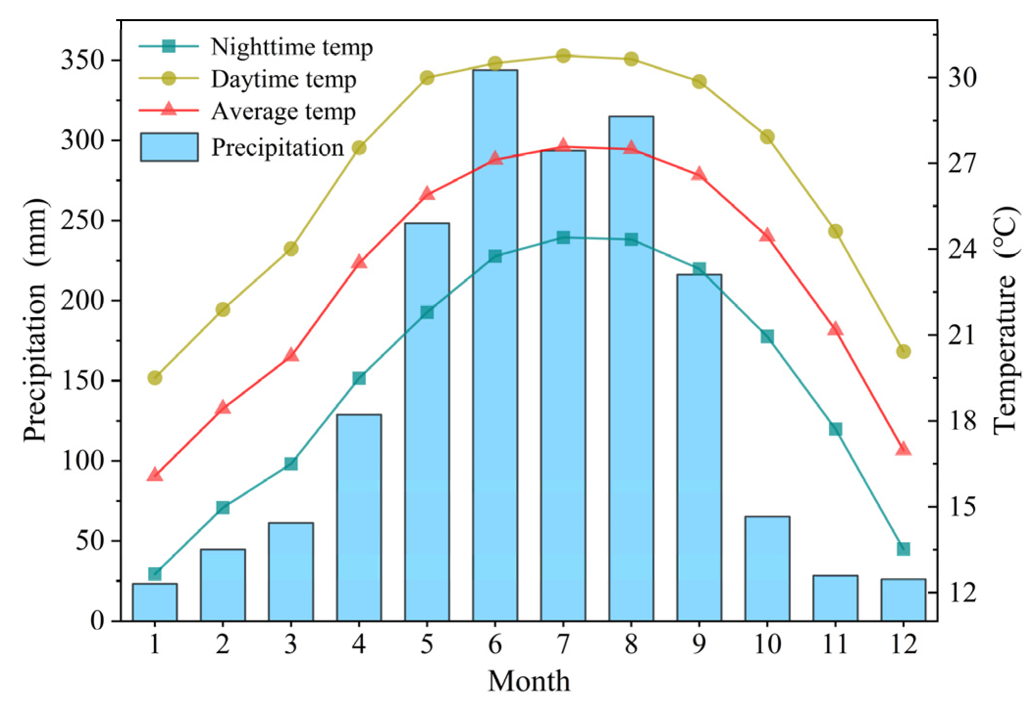
The annual changes of average temperature and precipitation in the study area from 1986 to 2020 were obtained from MOD11A1 version 006 and CHIRPS data, as shown in Figure 9. The study area has an obvious subtropical marine monsoon climate, with high temperature, rainy summers, and warm and humid winters. The highest temperatures occur in July, with an average day and night temperature of 27.59 °C, a daytime temperature of 30.76 °C, and a nighttime temperature of 24.41 °C. The lowest temperatures occurred in January, with an average day and night temperature of 16.08 °C, a daytime temperature of 19.51 °C, and a nighttime temperature of 12.64 °C. The precipitation in the rainy season (from April to September) accounts for 86.12% of the entire year.
A combined inspection of Figure 5 and Figure 9 reveals the intra-annual changes in temperature and precipitation consistent with nutrient concentrations. In the preceding analyses, we have approved that rivers greatly affect the water quality in the Shenzhen Bay. In summer, rising water temperature favors several transformations or actions related to water, such as dissolution, solubilization, complexation, degradation, and evaporation, which lead to changes in the concentration of dissolved substances in water [62]. At the same time, the temperature was positively associated with nitrification processes that increased the phosphatase activity and phosphorus mobilization in soil, and stimulated biological activity to increase nitrogen availability [63]. Thus, high temperatures and frequent droughts increased the mineralization and the release of nitrogen and phosphorus in soil organic matter. After heavy precipitation, these nutrients are washed into the streams and lead to higher nutrient concentrations in the river. Therefore, temperature and precipitation indirectly lead to intra-annual differences in water quality by affecting the water quality of rivers.
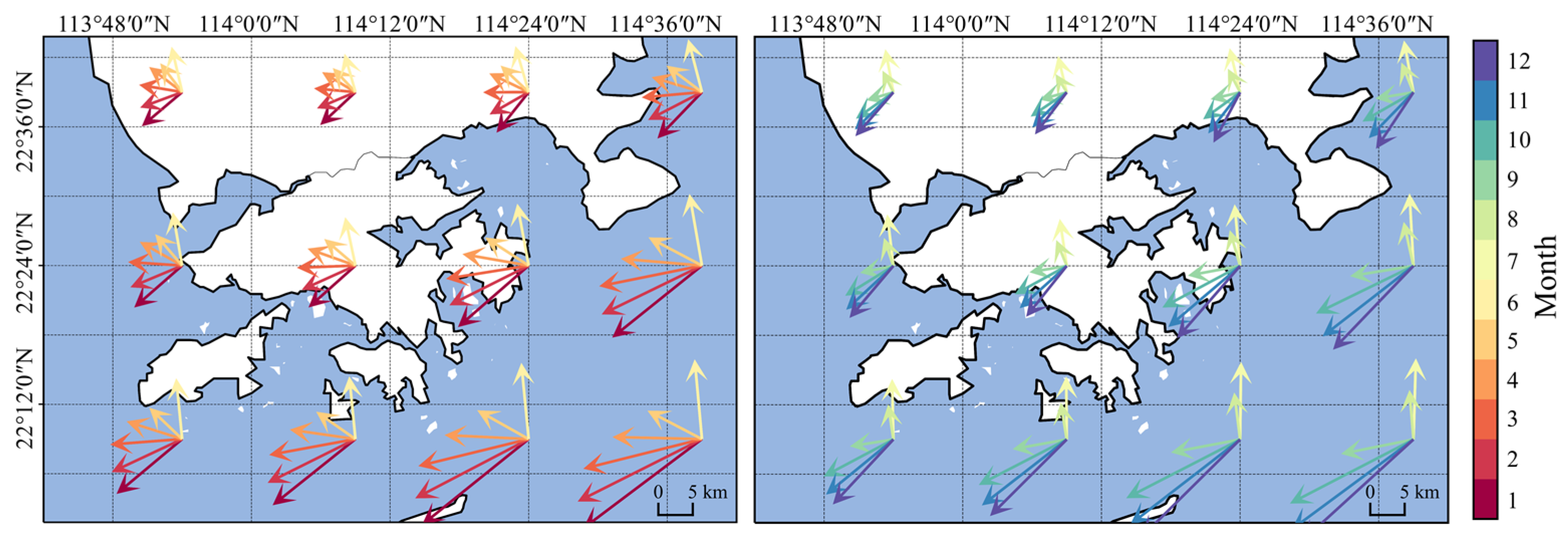
The monthly average direction and intensity information of wind in the study area from 1986 to 2021 was obtained from ERA5, as shown in Figure 10. The wind direction in the study area has a clear seasonality, with southwesterly winds prevailing in summer and northeasterly winds prevailing in winter. Seasonal changes in wind speed and direction are important for the control of the spread of the Pearl River plume [64]. During the dry season with wind speeds of 7–10 m/s, the plume is adverted westwards by northeasterly induced coastal currents, and the horizontal extent of the plume keeps narrow because of the low river flow. During the wet season, where wind speeds are generally less than 6 m/s, upwelling and southerly winds cause the high river discharge to be advected eastward and offshore. With high flow, the plume has a large horizontal extension [65]. The Pearl River Estuary water has been proven to have high nutrient concentrations [66], so the water from the Pearl River Estuary flowing to the vicinity of the Shenzhen Bay Estuary will also increase nutrient concentrations [67,68].

4.4. Impact of Oyster Farming

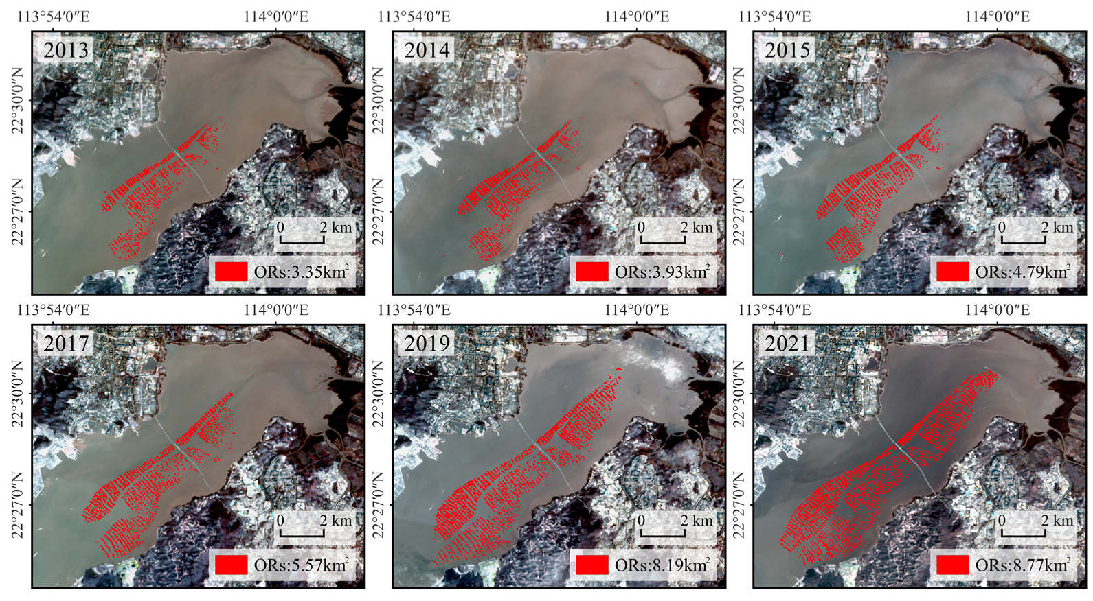
There are many oyster rafts (ORs) on the Hong Kong side of the Shenzhen Bay, especially in the area near Lau Fau Shan where fresh and salt water meet. Breeding methods using oyster rafts were introduced in the past ten years. Oysters remove nitrogen and phosphorus from the water by filtering and converting phytoplankton into shells and tissues, but also continuously expel these nutrients back into the water in the form of inorganic compounds [69]. Huang et al. [27] found that oyster farming in the Shenzhen Bay had little effect on dissolved inorganic nitrogen (DIN) and orthophosphate-phosphorous (PO4_P) concentrations.
We automatically extracted ORs using the MNDWI and Otsu methods using the averaged images of Landsat-8 from October to December in 2013–2021. The extraction results of ORs are shown in Figure 11. The ORs continued to expand to the northeast and southwest, from 3.35 km2 in 2013 to 8.77 km2 in 2021. However, with reference to Figure 3a,c, it was found that there was no abnormality in CTN and CTP around ORs.

4.5. Impact of Mangrove Forests

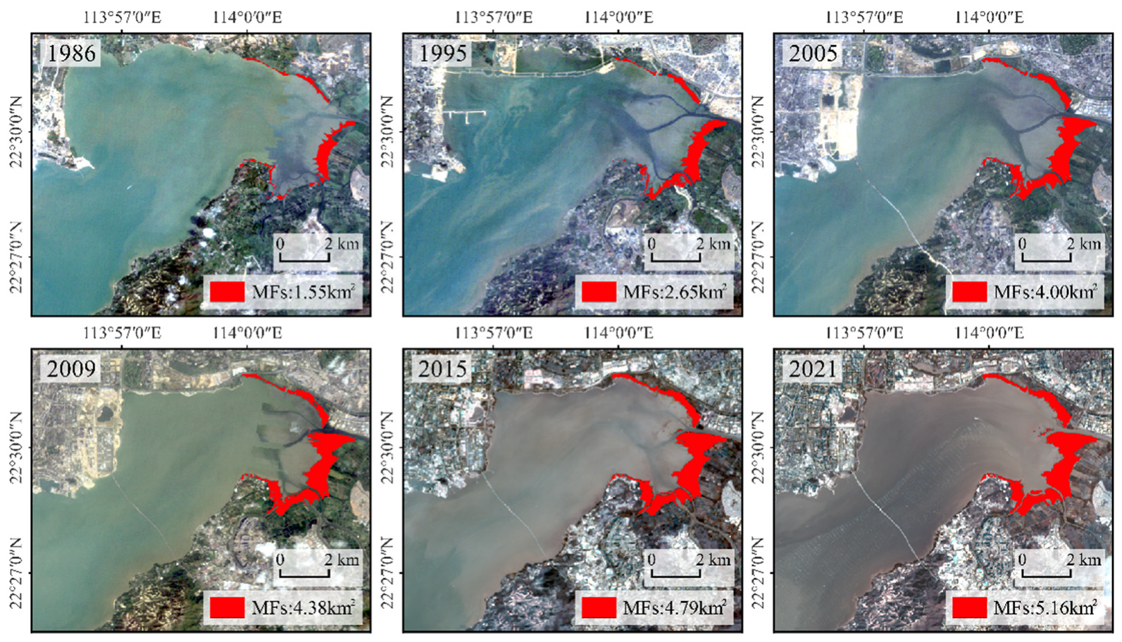
The mangrove forests (MFs) are mainly located in the northeast corner of the Shenzhen Bay and divided into two parts, the Futian Mangrove Reserve and the Mai Po Mangrove Reserve, bounded by the Shenzhen River. The Futian Mangrove Provincial Nature Reserve was established in 1984 and designated as a national nature reserve of China in 1988. In 1995, about 1500 hectares of wetland in Mai Po and Shenzhen Bay were designated as wetlands of international importance under the Ramsar Convention [70]. Due to the absorption of plants and microorganisms and the filtration of soil, mangrove wetlands have a good removal effect of nitrogen and phosphorus, but their growth is threatened when they exceed a certain threshold [71].
We computed the normalized difference vegetation index (NDVI) [72] which uses the red and the NIR band for the enhancement of vegetation canopies using averaged images of Landsat-5 and Landsat-8 from October to December in 1986–2021, and multiplied the NIR band to highlight the vegetation red-edge effects [73]. Then, we used the Otsu method to automatically extract thresholds to obtain MF areas. The results of extraction are shown in Figure 12. Overall, the MFs continue to expand to the ocean, with an area of 1.55 km2 in 1986 reaching 5.16 km2 in 2021. A combined view of Figure 3a,c reveals, even though MFs have a positive effect on the reduction of CTN and CTP, it is not a decisive factor for changes.

5. Conclusions

In this study, we constructed an inversion model of TN and TP for the boundary waters of Shenzhen and Hong Kong using Landsat-5/8 images and measured in situ data from 1986 to 2020. Comparing four different machine learning methods (TE, SVM, GPR, BPNN), it turned out that the BPNN performed best, proven by calculated parameters such as the r, R2, MAE, and RMSE. The inversion results show that the CTN and CTP in the Shenzhen Bay, the Starling Inlet, and the Tolo Harbor were relatively high, fluctuated from 1986 to 2010, and decreased significantly after 2010. The CTN and CTP in the Mirs Bay remained continuously at a low level. The data refer to urbanization processes and polluted river discharges as the main driving factors for both spatial and inter-annual differences of CTN and CTP. Furthermore, temperature, precipitation, and the impact of wind had a great influence on the intra-annual changes of CTN and CTP in the Shenzhen Bay.
Although machine learning methods have improved the accuracy of inversion, there are still some limitations to be mentioned. One of the most influencing factors is the optical complexity of coastal waters due to their varying trophic levels triggered by suspended matter and phytoplankton. Further constraints may be introduced by insufficient atmospheric corrections, BRDF effects due to seasonally varying irradiation angles of the Sun, and the precision of given gain and offset values of the respective datasets. All these parameters directly affect the inversion results, and the regional generalization ability of the model. Future investigations are focused on the use of upcoming hyperspectral satellite data, which should further improve the quality of results, and on a more detailed evaluation of the respective drivers. The importance of such type of investigations based on satellite data and machine learning methods is widely recognized as they are an indispensable tool to synoptically and more precisely monitor and manage the quality of coastal water bodies.
In summary, this study provides a methodological reference for the inversion of non-optical activity parameters of coastal waters, and confirms that remote sensing is a reliable and robust tool for water quality monitoring and comprehensive analysis of driving forces at spatiotemporal scales.

Author Contributions

Conceptualization, H.L. and G.Z.; Data curation, H.L.; Formal analysis, H.L.; Funding acquisition, G.X.; Investigation, H.L. and G.Z.; Methodology, H.L., G.Z. and Y.Z.; Project administration, G.X.; Resources, G.X.; Software, H.L., G.Z. and Y.Z.; Supervision, G.X.; Validation, H.L.; Visualization, H.L. and Y.Z.; Writing—original draft, H.L.; Writing—review & editing, H.K. All authors have read and agreed to the published version of the manuscript.

Funding

This research was funded by the Shenzhen Science and Technology Program (Grant No. KQTD20180410161218820), the Guangdong Basic and Applied Basic Research Foundation (2021A1515012600), the Opening Project of Guangxi Wireless Broadband Communication and Signal Processing Key Laboratory (No. GXKL06200217) and the Open Fund of Key Laboratory of Urban Land Resources Monitoring and Simulation, Ministry of Natural Resources (KF-2021-06-104).

Data Availability Statement

The measured water quality data are available from HKEPD (https://www.epd.gov.hk/epd/sc_chi/environmentinhk/water/hkwqrc/waterquality/marine.html) (accessed on 1 January 2022). The surface reflectance datasets of Landsat, MOD11A1, and CHIRPS are available on GEE (https://earthengine.google.com) (accessed on 1 January 2022). GISA dataset can be accessed via this link (https://zenodo.org/record/5136330#.Yq1o7-hByUk) (accessed on 15 March 2022). ERA5 monthly averaged data can be downloaded through this link (https://cds.climate.copernicus.eu/cdsapp#!/home) (accessed on 10 April 2022).

Acknowledgments

We thank the developers for their tools and the respective agencies that provided the data. We further thank all editors and anonymous reviewers for spending their time working on the manuscript.

Conflicts of Interest

The authors declare no conflict of interest.

References

  1. Neumann, B.; Vafeidis, A.T.; Zimmermann, J.; Nicholls, R.J. Future Coastal Population Growth and Exposure to Sea-Level Rise and Coastal Flooding—A Global Assessment. PLoS ONE 2015, 10, e0118571. [Google Scholar] [CrossRef] [Green Version]
  2. Kitamori, K.; Manders, T.; Dellink, R.; Tabeau, A. OECD Environmental Outlook to 2050: The Consequences of Inaction; 9264122168; OECD: Paris, France, 2012. [Google Scholar]
  3. World Health Organization; UNICEF. Meeting the MDG Drinking Water and Sanitation Target: The Urban and Rural Challenge of the Decade; World Health Organization: Geneva, Switzerland; UNICEF: New York, NY, USA, 2006. [Google Scholar]
  4. Ritchie, J.C.; Zimba, P.V.; Everitt, J.H. Remote sensing techniques to assess water quality. Photogramm. Eng. Remote Sens. 2003, 69, 695–704. [Google Scholar] [CrossRef] [Green Version]
  5. Mouw, C.B.; Greb, S.; Aurin, D.; DiGiacomo, P.M.; Lee, Z.; Twardowski, M.; Binding, C.; Hu, C.; Ma, R.; Moore, T.; et al. Aquatic color radiometry remote sensing of coastal and inland waters: Challenges and recommendations for future satellite missions. Remote Sens. Environ. 2015, 160, 15–30. [Google Scholar] [CrossRef]
  6. Doña, C.; Sánchez, J.M.; Caselles, V.; Domínguez, J.A.; Camacho, A. Empirical relationships for monitoring water quality of lakes and reservoirs through multispectral images. IEEE J. Sel. Top. Appl. Earth Obs. Remote Sens. 2014, 7, 1632–1641. [Google Scholar] [CrossRef]
  7. Härmä, P.; Vepsäläinen, J.; Hannonen, T.; Pyhälahti, T.; Kämäri, J.; Kallio, K.; Eloheimo, K.; Koponen, S. Detection of water quality using simulated satellite data and semi-empirical algorithms in Finland. Sci. Total Environ. 2001, 268, 107–121. [Google Scholar] [CrossRef]
  8. Gordon, H.R.; Brown, O.B.; Jacobs, M.M. Computed Relationships Between the Inherent and Apparent Optical Properties of a Flat Homogeneous Ocean. Appl. Opt. 1975, 14, 417–427. [Google Scholar] [CrossRef]
  9. Dall’Olmo, G.; Gitelson, A.A.; Rundquist, D.C. Towards a unified approach for remote estimation of chlorophyll-a in both terrestrial vegetation and turbid productive waters. Geophys. Res. Lett. 2003, 30, 1938. [Google Scholar] [CrossRef] [Green Version]
  10. Chacon-Torres, A.; Ross, L.G.; Beveridge, M.C.M.; Watson, A.I. The application of SPOT multispectral imagery for the assessment of water quality in Lake Patzcuaro, Mexico. Int. J. Remote Sens. 1992, 13, 587–603. [Google Scholar] [CrossRef]
  11. Lim, J.; Choi, M. Assessment of water quality based on Landsat 8 operational land imager associated with human activities in Korea. Environ. Monit. Assess. 2015, 187, 384. [Google Scholar] [CrossRef]
  12. Gholizadeh, M.H.; Melesse, A.M.; Reddi, L. A Comprehensive Review on Water Quality Parameters Estimation Using Remote Sensing Techniques. Sensors 2016, 16, 1298. [Google Scholar] [CrossRef] [Green Version]
  13. Sagan, V.; Peterson, K.T.; Maimaitijiang, M.; Sidike, P.; Sloan, J.; Greeling, B.A.; Maalouf, S.; Adams, C. Monitoring inland water quality using remote sensing: Potential and limitations of spectral indices, bio-optical simulations, machine learning, and cloud computing. Earth-Sci. Rev. 2020, 205, 103187. [Google Scholar] [CrossRef]
  14. Niu, C.; Tan, K.; Jia, X.; Wang, X. Deep learning based regression for optically inactive inland water quality parameter estimation using airborne hyperspectral imagery. Environ. Pollut. 2021, 286, 117534. [Google Scholar] [CrossRef] [PubMed]
  15. Paerl, H.W.; Otten, T.G. Harmful Cyanobacterial Blooms: Causes, Consequences, and Controls. Microb. Ecol. 2013, 65, 995–1010. [Google Scholar] [CrossRef] [PubMed]
  16. Carlson, R.E. A trophic state index for lakes1. Limnol. Oceanogr. 1977, 22, 361–369. [Google Scholar] [CrossRef] [Green Version]
  17. Li, Y.; Zhang, Y.; Shi, K.; Zhu, G.; Zhou, Y.; Zhang, Y.; Guo, Y. Monitoring spatiotemporal variations in nutrients in a large drinking water reservoir and their relationships with hydrological and meteorological conditions based on Landsat 8 imagery. Sci. Total Environ. 2017, 599–600, 1705–1717. [Google Scholar] [CrossRef] [PubMed]
  18. Sun, X.; Zhang, Y.; Shi, K.; Zhang, Y.; Li, N.; Wang, W.; Huang, X.; Qin, B. Monitoring water quality using proximal remote sensing technology. Sci. Total Environ. 2022, 803, 149805. [Google Scholar] [CrossRef]
  19. Mathew, M.M.; Srinivasa Rao, N.; Mandla, V.R. Development of regression equation to study the Total Nitrogen, Total Phosphorus and Suspended Sediment using remote sensing data in Gujarat and Maharashtra coast of India. J. Coast. Conserv. 2017, 21, 917–927. [Google Scholar] [CrossRef]
  20. Gao, Y.; Gao, J.; Yin, H.; Liu, C.; Xia, T.; Wang, J.; Huang, Q. Remote sensing estimation of the total phosphorus concentration in a large lake using band combinations and regional multivariate statistical modeling techniques. J. Environ. Manag. 2015, 151, 33–43. [Google Scholar] [CrossRef]
  21. Dong, G.; Hu, Z.; Liu, X.; Fu, Y.; Zhang, W. Spatio-Temporal Variation of Total Nitrogen and Ammonia Nitrogen in the Water Source of the Middle Route of the South-To-North Water Diversion Project. Water 2020, 12, 2615. [Google Scholar] [CrossRef]
  22. Vakili, T.; Amanollahi, J. Determination of optically inactive water quality variables using Landsat 8 data: A case study in Geshlagh reservoir affected by agricultural land use. J. Clean. Prod. 2020, 247, 119134. [Google Scholar] [CrossRef]
  23. Xiong, J.; Lin, C.; Cao, Z.; Hu, M.; Xue, K.; Chen, X.; Ma, R. Development of remote sensing algorithm for total phosphorus concentration in eutrophic lakes: Conventional or machine learning? Water Res. 2022, 215, 118213. [Google Scholar] [CrossRef] [PubMed]
  24. Hafeez, S.; Wong, M.S.; Ho, H.C.; Nazeer, M.; Nichol, J.; Abbas, S.; Tang, D.; Lee, K.H.; Pun, L. Comparison of Machine Learning Algorithms for Retrieval of Water Quality Indicators in Case-II Waters: A Case Study of Hong Kong. Remote Sens. 2019, 11, 617. [Google Scholar] [CrossRef] [Green Version]
  25. Qiao, Z.; Sun, S.; Jiang, Q.O.; Xiao, L.; Wang, Y.; Yan, H. Retrieval of Total Phosphorus Concentration in the Surface Water of Miyun Reservoir Based on Remote Sensing Data and Machine Learning Algorithms. Remote Sens. 2021, 13, 4662. [Google Scholar] [CrossRef]
  26. Qun’ou, J.; Lidan, X.; Siyang, S.; Meilin, W.; Huijie, X. Retrieval model for total nitrogen concentration based on UAV hyper spectral remote sensing data and machine learning algorithms—A case study in the Miyun Reservoir, China. Ecol. Indic. 2021, 124, 107356. [Google Scholar] [CrossRef]
  27. Huang, J.; Wang, D.; Gong, F.; Bai, Y.; He, X. Changes in Nutrient Concentrations in Shenzhen Bay Detected Using Landsat Imagery between 1988 and 2020. Remote Sens. 2021, 13, 3469. [Google Scholar] [CrossRef]
  28. Wang, C.; Li, W.; Chen, S.; Li, D.; Wang, D.; Liu, J. The spatial and temporal variation of total suspended solid concentration in Pearl River Estuary during 1987–2015 based on remote sensing. Sci. Total Environ. 2018, 618, 1125–1138. [Google Scholar] [CrossRef]
  29. Nazeer, M.; Nichol, J.E. Combining Landsat TM/ETM+ and HJ-1 A/B CCD Sensors for Monitoring Coastal Water Quality in Hong Kong. IEEE Geosci. Remote Sens. Lett. 2015, 12, 1898–1902. [Google Scholar] [CrossRef]
  30. Feng, T.; Xu, N. Satellite-Based Monitoring of Annual Coastal Reclamation in Shenzhen and Hong Kong since the 21st Century: A Comparative Study. J. Mar. Sci. Eng. 2021, 9, 48. [Google Scholar] [CrossRef]
  31. Huang, X.; Li, J.; Yang, J.; Zhang, Z.; Li, D.; Liu, X. 30 m global impervious surface area dynamics and urban expansion pattern observed by Landsat satellites: From 1972 to 2019. Sci. China Earth Sci. 2021, 64, 1922–1933. [Google Scholar] [CrossRef]
  32. Funk, C.; Peterson, P.; Landsfeld, M.; Pedreros, D.; Verdin, J.; Shukla, S.; Husak, G.; Rowland, J.; Harrison, L.; Hoell, A.; et al. The climate hazards infrared precipitation with stations—A new environmental record for monitoring extremes. Sci. Data 2015, 2, 150066. [Google Scholar] [CrossRef] [Green Version]
  33. Hersbach, H.; Bell, B.; Berrisford, P.; Biavati, G.; Horányi, A.; Muñoz Sabater, J.; Nicolas, J.; Peubey, C.; Radu, R.; Rozum, I.; et al. ERA5 monthly averaged data on single levels from 1959 to present. In Copernicus Climate Change Service (C3S) Climate Data Store (CDS); Available online: https://cds.climate.copernicus.eu/cdsapp#!/dataset/10.24381/cds.f17050d7?tab=overview (accessed on 10 April 2022).
  34. Xu, H. Modification of normalised difference water index (NDWI) to enhance open water features in remotely sensed imagery. Int. J. Remote Sens. 2006, 27, 3025–3033. [Google Scholar] [CrossRef]
  35. Otsu, N. A Threshold Selection Method from Gray-Level Histograms. IEEE Trans. Syst. Man Cybern. 1979, 9, 62–66. [Google Scholar] [CrossRef] [Green Version]
  36. Breiman, L.; Friedman, J.H.; Olshen, R.A.; Stone, C.J. Classification and Regression Trees; Routledge: London, UK, 1984. [Google Scholar]
  37. Sutton, C.D. 11—Classification and Regression Trees, Bagging, and Boosting. In Handbook of Statistics; Rao, C.R., Wegman, E.J., Solka, J.L., Eds.; Elsevier: Amsterdam, The Netherlands, 2005; Volume 24, pp. 303–329. [Google Scholar]
  38. Smola, A.J.; Schölkopf, B. A tutorial on support vector regression. Stat. Comput. 2004, 14, 199–222. [Google Scholar] [CrossRef] [Green Version]
  39. Vapnik, V. The Nature of Statistical Learning Theory; Springer Science & Business Media: Berlin/Heidelberg, Germany, 1999. [Google Scholar]
  40. An, C.; Xie, C.; Meng, Y.; Shi, X.; Yang, C. Large Deformation Modeling of Wing-Like Structures Based on Support Vector Regression. Appl. Sci. 2020, 10, 5995. [Google Scholar] [CrossRef]
  41. Dibike, Y.B.; Velickov, S.; Solomatine, D.; Abbott Michael, B. Model Induction with Support Vector Machines: Introduction and Applications. J. Comput. Civ. Eng. 2001, 15, 208–216. [Google Scholar] [CrossRef]
  42. Verrelst, J.; Muñoz, J.; Alonso, L.; Delegido, J.; Rivera, J.P.; Camps-Valls, G.; Moreno, J. Machine learning regression algorithms for biophysical parameter retrieval: Opportunities for Sentinel-2 and -3. Remote Sens. Environ. 2012, 118, 127–139. [Google Scholar] [CrossRef]
  43. Yuan, J.; Wang, K.; Yu, T.; Fang, M. Reliable multi-objective optimization of high-speed WEDM process based on Gaussian process regression. Int. J. Mach. Tools Manuf. 2008, 48, 47–60. [Google Scholar] [CrossRef]
  44. Rumelhart, D.E.; Hinton, G.E.; Williams, R.J. Learning representations by back-propagating errors. Nature 1986, 323, 533–536. [Google Scholar] [CrossRef]
  45. Widrow, B.; Rumelhart, D.E.; Lehr, M.A. Neural networks: Applications in industry, business and science. Commun. ACM 1994, 37, 93–105. [Google Scholar] [CrossRef]
  46. Refaeilzadeh, P.; Tang, L.; Liu, H. Cross-validation. Encycl. Database Syst. 2009, 5, 532–538. [Google Scholar]
  47. Yang, L.; Shami, A. On hyperparameter optimization of machine learning algorithms: Theory and practice. Neurocomputing 2020, 415, 295–316. [Google Scholar] [CrossRef]
  48. Wu, J.; Chen, X.-Y.; Zhang, H.; Xiong, L.-D.; Lei, H.; Deng, S.-H. Hyperparameter Optimization for Machine Learning Models Based on Bayesian Optimizationb. J. Electron. Sci. Technol. 2019, 17, 26–40. [Google Scholar] [CrossRef]
  49. Liu, Z.; Wang, Y.; Li, Z.; Peng, J. Impervious surface impact on water quality in the process of rapid urbanization in Shenzhen, China. Environ. Earth Sci. 2013, 68, 2365–2373. [Google Scholar] [CrossRef]
  50. Luo, Y.; Zhao, Y.; Yang, K.; Chen, K.; Pan, M.; Zhou, X. Dianchi Lake watershed impervious surface area dynamics and their impact on lake water quality from 1988 to 2017. Environ. Sci. Pollut. Res. 2018, 25, 29643–29653. [Google Scholar] [CrossRef]
  51. He, L.; Wang, J.; Liu, Y.; Zhang, Y.; He, C.; Yu, Q.; Ma, W. Selection of onshore sites based on monitoring possibility evaluation of exhausts from individual ships for Yantian Port, China. Atmos. Environ. 2021, 247, 118187. [Google Scholar] [CrossRef]
  52. Shaikh, S.M.S.; Tagde, J.P.; Singh, P.R.; Dutta, S.; Sangolkar, L.N.; Kumar, M.S. Impact of Port and harbour activities on plankton distribution and dynamics: A multivariate approach. Mar. Pollut. Bull. 2021, 165, 112105. [Google Scholar] [CrossRef]
  53. Le Moal, M.; Gascuel-Odoux, C.; Ménesguen, A.; Souchon, Y.; Étrillard, C.; Levain, A.; Moatar, F.; Pannard, A.; Souchu, P.; Lefebvre, A.; et al. Eutrophication: A new wine in an old bottle? Sci. Total Environ. 2019, 651, 1–11. [Google Scholar] [CrossRef] [Green Version]
  54. Wang, G.; Zhang, B.; Li, J.; Zhang, H.; Shen, Q.; Wu, D.; Song, Y. Study on Monitoring of Red Tide by Multi-Spectral Remote Sensing Based on HJ-CCD and MODIS. Procedia Environ. Sci. 2011, 11, 1561–1565. [Google Scholar] [CrossRef] [Green Version]
  55. Yudhistira, M.H.; Karimah, I.D.; Maghfira, N.R. The effect of port development on coastal water quality: Evidence of eutrophication states in Indonesia. Ecol. Econ. 2022, 196, 107415. [Google Scholar] [CrossRef]
  56. Sin, Y.S.; Chau, K.W. Eutrophication Studies on Tolo Harbour, Hong Kong. Water Sci. Technol. 1992, 26, 2551–2554. [Google Scholar] [CrossRef]
  57. HKEPD. Regional Collaboration with Shenzhen in Deep Bay (Shenzhen Bay). Available online: https://www.epd.gov.hk/epd/english/environmentinhk/water/hkwqrc/regional/deepbay.html (accessed on 5 May 2022).
  58. Bureau, S.M.E.A.E. Annual Environmental Status Bulletin. Available online: http://meeb.sz.gov.cn/xxgk/tjsj/ndhjzkgb (accessed on 5 May 2022).
  59. Deng, T.; Duan, H.-F.; Keramat, A. Spatiotemporal characterization and forecasting of coastal water quality in the semi-enclosed Tolo Harbour based on machine learning and EKC analysis. Eng. Appl. Comput. Fluid Mech. 2022, 16, 694–712. [Google Scholar] [CrossRef]
  60. Deng, T.; Chau, K.-W.; Duan, H.-F. Machine learning based marine water quality prediction for coastal hydro-environment management. J. Environ. Manag. 2021, 284, 112051. [Google Scholar] [CrossRef] [PubMed]
  61. HKEPD. Annual Marine Water Quality Reports. Available online: https://www.epd.gov.hk/epd/english/environmentinhk/water/hkwqrc/waterquality/marine-2.html (accessed on 5 May 2022).
  62. Delpla, I.; Jung, A.V.; Baures, E.; Clement, M.; Thomas, O. Impacts of climate change on surface water quality in relation to drinking water production. Environ. Int. 2009, 35, 1225–1233. [Google Scholar] [CrossRef]
  63. Sardans, J.; Peñuelas, J.; Estiarte, M. Changes in soil enzymes related to C and N cycle and in soil C and N content under prolonged warming and drought in a Mediterranean shrubland. Appl. Soil Ecol. 2008, 39, 223–235. [Google Scholar] [CrossRef]
  64. Dong, L.; Su, J.; Ah Wong, L.; Cao, Z.; Chen, J.-C. Seasonal variation and dynamics of the Pearl River plume. Cont. Shelf Res. 2004, 24, 1761–1777. [Google Scholar] [CrossRef]
  65. Harrison, P.J.; Yin, K.; Lee, J.H.W.; Gan, J.; Liu, H. Physical–biological coupling in the Pearl River Estuary. Cont. Shelf Res. 2008, 28, 1405–1415. [Google Scholar] [CrossRef]
  66. Zhao, Y.; Song, Y.; Cui, J.; Gan, S.; Yang, X.; Wu, R.; Guo, P. Assessment of Water Quality Evolution in the Pearl River Estuary (South Guangzhou) from 2008 to 2017. Water 2020, 12, 59. [Google Scholar]
  67. Ou, S.; Yang, Q.; Luo, X.; Zhu, F.; Luo, K.; Yang, H. The influence of runoff and wind on the dispersion patterns of suspended sediment in the Zhujiang (Pearl) River Estuary based on MODIS data. Acta Oceanol. Sin. 2019, 38, 26–35. [Google Scholar] [CrossRef]
  68. Kedong, Y. Monsoonal influence on seasonal variations in nutrients and phytoplankton biomass in coastal waters of Hong Kong in the vicinity of the Pearl River estuary. Mar. Ecol. Prog. Ser. 2002, 245, 111–122. [Google Scholar]
  69. Ray, N.E.; Li, J.; Kangas, P.C.; Terlizzi, D.E. Water quality upstream and downstream of a commercial oyster aquaculture facility in Chesapeake Bay, USA. Aquac. Eng. 2015, 68, 35–42. [Google Scholar] [CrossRef]
  70. Feng, Z.; Tan, G.; Xia, J.; Shu, C.; Chen, P.; Wu, M.; Wu, X. Dynamics of mangrove forests in Shenzhen Bay in response to natural and anthropogenic factors from 1988 to 2017. J. Hydrol. 2020, 591, 125271. [Google Scholar] [CrossRef]
  71. Lotfinasabasl, S.; Gunale, V.R.; Khosroshahi, M. Applying geographic information systems and remote sensing for water quality assessment of mangrove forest. Acta Ecol. Sin. 2018, 38, 135–143. [Google Scholar] [CrossRef]
  72. Rouse, J.W.; Haas, R.H.; Schell, J.A.; Deering, D.W. Monitoring vegetation systems in the great plains with ERTS. In Proceedings of the Third ERTS Symposium, NASA SP-351, I, Washington, DC, USA, 10–14 December 1973; pp. 309–317. [Google Scholar]
  73. Filella, I.; Penuelas, J. The red edge position and shape as indicators of plant chlorophyll content, biomass and hydric status. Int. J. Remote Sens. 1994, 15, 1459–1470. [Google Scholar] [CrossRef]
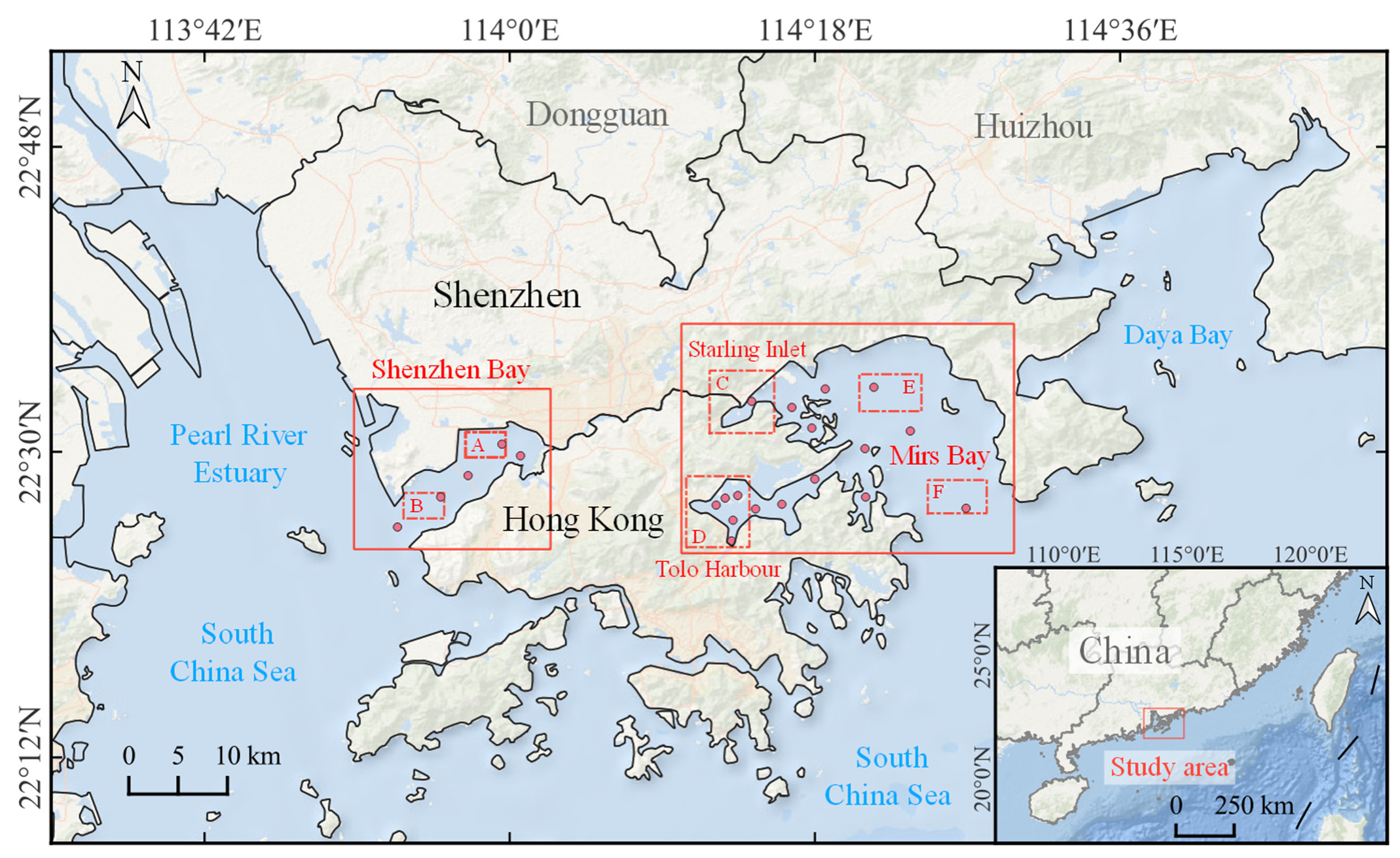
Figure 1. Map of the study area and the monitoring areas (A–F). Red dots = stations.
Remotesensing 14 03694 g001
Figure 2. Performance evaluation of the Back-propagation Neural Network (BPNN) using all data.
Remotesensing 14 03694 g002
Figure 3. Spatial distribution of total nitrogen (TN) and total phosphorus (TP) in (a,c) the western part and (b,d) the eastern part of the study area.
Remotesensing 14 03694 g003aRemotesensing 14 03694 g003b
Figure 4. Inter-annual changes of (a) TN and (b) TP concentrations within the monitoring areas (A–F).
Remotesensing 14 03694 g004
Figure 5. Intra-annual changes of (a) TN and (b) TP concentrations within the monitoring areas (A–F).
Remotesensing 14 03694 g005
Figure 6. Spatiotemporal changes of impervious surface areas (ISA) and coastlines. (a) Location of the monitoring areas (I, II and III). (b,c) Shekou Peninsula. (d,e) Yantian Port.
Remotesensing 14 03694 g006
Figure 7. Inter-annual changes of (a) the ISA and (b) the increase in ISA within the monitoring areas (I, II, and III).
Remotesensing 14 03694 g007
Figure 8. Inversion results of TN (af) and TP (gl) in the Yantian Port.
Remotesensing 14 03694 g008
Figure 9. Intra-annual changes of temperature and precipitation.
Remotesensing 14 03694 g009
Figure 10. The monthly average direction and intensity of winds from 1986 to 2021. Arrows represent wind directions. The lengths of the arrows represent the wind speed.
Remotesensing 14 03694 g010
Figure 11. Inter-annual changes of the location and distribution of oyster rafts (ORs) in the Shenzhen Bay from 2013 to 2021.
Remotesensing 14 03694 g011
Figure 12. Inter-annual changes of the location and distribution of mangrove forests (MFs) in the Shenzhen Bay from 1986 to 2021.
Remotesensing 14 03694 g012
Table 1. Best hyperparameter combinations for the respective methods of Tree Embedding (TE), Support Vector Regression (SVR), Gaussian Process Regression (GPR), and Back-propagation Neural Network (BPNN).
MethodHyperparameterTN-L5TN-L8TP-L5TP-L8
TEEnsemble methodLS BoostLS BoostLS BoostBag
Isotropic Exponential4481839928
Learning rate0.13430.48490.0254/
Minimum leaf size2122
SVMKernel functionGaussianQuadraticQuadraticLinear
Box constraint79.61260.08141.57650.6258
Kernel scale2.3638///
Epsilon0.39722.49 × 10−40.11250.0048
GPRBasis functionConstantLinearZeroLinear
Kernel functionNon-isotropic Rational QuadraticNon-isotropic Matem 3/2Isotropic ExponentialIsotropic Matem 5/2
Kernel scale1988.3/1114.73.46
Sigma1.89 × 10−40.09780.10810.0066
BPNNActivationReLUReLUReLUSigmoid
Number of layers2223
Regularization strength (Lambda)0.01430.00590.00072.95 × 10−5
Number of neurons in the first hidden layer8225647139
Number of neurons in the second hidden layer11510134
Number of neurons in the third hidden layer///4
Table 2. Accuracy values of the TE, SVM, GPR and BPNN methods.
ModelMethod5-foldTraining SetTest SetAll Data
RMSErR2MAERMSErR2MAERMSErR2MAERMSE
TN-L5TE0.851.000.990.070.100.760.570.521.190.920.850.160.54
SVR0.920.830.680.400.750.730.530.571.280.800.630.440.88
GPR0.851.001.000.000.000.800.630.461.110.940.880.090.50
BPNN0.830.860.730.380.670.790.620.511.130.830.700.410.78
TN-L8TE0.450.990.980.070.090.570.320.330.710.900.810.120.33
SVR0.330.920.850.180.300.730.530.270.540.860.740.200.36
GPR0.340.980.960.110.140.700.490.280.590.920.840.140.29
BPNN0.350.960.930.140.200.820.670.240.510.920.840.160.29
TP-L5TE0.140.940.890.040.070.710.510.090.190.870.760.050.10
SVR0.140.610.370.090.150.680.470.110.210.630.400.090.17
GPR0.141.001.000.000.000.760.580.080.180.930.860.020.08
BPNN0.140.870.750.060.100.770.600.080.170.840.700.060.12
TP-L8TE0.050.920.840.010.030.650.420.030.050.850.730.020.04
SVR0.050.730.530.020.050.760.580.020.040.730.540.020.05
GPR0.050.950.890.020.020.680.460.030.060.870.760.020.04
BPNN0.050.920.850.020.030.790.630.020.040.900.810.020.03
Publisher’s Note: MDPI stays neutral with regard to jurisdictional claims in published maps and institutional affiliations.