Disentangling Soil, Shade, and Tree Canopy Contributions to Mixed Satellite Vegetation Indices in a Sparse Dry Forest

Abstract

Remote sensing (RS) for vegetation monitoring can involve mixed pixels with contributions from vegetation and background surfaces, causing biases in signals and their interpretations, especially in low-density forests. In a case study in the semi-arid Yatir forest in Israel, we observed a mismatch between satellite (Landsat 8 surface product) and tower-based (Skye sensor) multispectral data and contrasting seasonal cycles in near-infrared (NIR) reflectance. We tested the hypothesis that this mismatch was due to the different fractional contributions of the various surface components and their unique reflectance. Employing an unmanned aerial vehicle (UAV), we obtained high-resolution multispectral images over selected forest plots and estimated the fraction, reflectance, and seasonal cycle of the three main surface components (canopy, shade, and sunlit soil). We determined that the Landsat 8 data were dominated by soil signals (70%), while the tower-based data were dominated by canopy signals (95%). We then developed a procedure to resolve the canopy (i.e., tree foliage) normalized difference vegetation index (NDVI) from the mixed satellite data. The retrieved and corrected canopy-only data resolved the original mismatch and indicated that the spatial variations in Landsat 8 NDVI were due to differences in stand density, while the canopy-only NDVI was spatially uniform, providing confidence in the local flux tower measurements.

1. Introduction

Remote sensing (RS) has been shown to have great potential and advantages in earth surface monitoring for several decades [1,2,3]. Most of the current satellites have low to moderate spatial resolution, meaning that one pixel usually contains a mixture of vegetation (tree and understory) and background (soil, shade, etc.), which is known as the mixed-pixel problem [4,5,6]. This issue is particularly significant for semi-arid and dryland ecosystems where the vegetation is usually sparse [7]. Compared to dense canopy forests, RS applications in sparse semi-arid forests face the need to consider the multiple components within a pixel, especially considering the forest mortalities that are induced by global warming [8,9,10]. Generally, vegetation has a low reflectance due to the pigment absorption in the radiative photosynthetic range and high reflectance in the near-infrared (NIR) range that is related to canopy structure [11]. The soil reflectance spectrum has less contrast along the wavelength and is strongly related to soil water content, soil composition, and surface roughness [12,13]. For sites with homogeneous soil types, the soil water content is the dominating factor for soil reflectance, with lower surface reflectance commonly observed in wetter soil, at low moisture levels, and in the visible to shortwave infrared domains [13,14,15,16,17]. This phenomenon can be explained as internal reflection that is caused by the water film covering soil particles, which ultimately reach other soil particles and are absorbed again. Therefore, vegetation and non-vegetation components strongly influence each mixed pixel’s spectral information.

Many vegetation indices (VIs) have been developed to extract vegetation parameters from space; these VIs mainly use the visible and NIR bands [18,19,20,21]. To date, the normalized difference vegetation index (NDVI) is the most widely-used VI, but the NDVI value can vary significantly when the background soil reflectance changes due to, for example, soil moisture content [22,23]. Approaches for solving this problem include reducing soil signals at low vegetation cover by adding soil brightness correction factors (SAVI, MSAVI2, OSAVI, GSAVI) [24,25,26,27] or enhancing vegetation signals at high vegetation cover by adding weighting coefficients (EVI, WDRVI, NIRv) [20,21,28]. However, these indices that are derived from most satellites still may not accurately capture surface phenological changes due to their limited spatial resolutions [6]. In addition, shade also causes biased NDVI values, thus significantly reducing land cover classification accuracy. The NDVI of a shaded area can be higher or lower than that of a sunlit region depending on the surface type, the objects that cast the shade, and the darkness of the shadow [29,30,31]. Due to these complexities, little work has been published on correcting shade influences in vegetation indices.

Ground multispectral instruments provide another possibility to measure the ecosystem VIs closely. The comparison between satellites and ground multispectral data has been reported to be consistent with the possible effects of ecosystem type and characteristics, or with atmospheric effects [32,33]. Measurements from ground radiometers, such as those on Eddy Covariance towers, mainly measure the canopy top and the canopy side in sparse ecosystems due to their close distance to the crown and wider viewing angle [34]. In contrast, the nadir view of satellites and their large pixel size lead to non-negligible contributions from the large proportions of sunlit and shaded soil [35]. These effects are most pronounced in sparse ecosystems, thus adding complexity to comparisons between the two RS measurements. Attempts to understand the individual contributions of the surface elements from such mixed pixels require high-resolution multispectral images and accurate image classification algorithms.

In recent years, multispectral cameras that were installed on unmanned aerial vehicles (UAVs) have been used widely in forest RS applications [36,37,38]. Due to the high resolutions of UAVs, the accuracy of canopy segmentation has been dramatically improved by using thresholds in canopy height [39] or vegetation indices [38,40]. Classifying shaded areas, which previously required comprehensive modeling [31,41,42], was also significantly improved by simple thresholds in reflectance [43]. To date, most UAV studies have mainly focused on calibrating/improving image segmentation algorithms or extracting the canopy information after classification [44,45]. For sparse dryland ecosystems with large exposed soil areas, studying the fractional contributions of each surface component is important [46,47].

Forests in dryland habitats cover more than 40% of the Earth’s land surface [48]. Due to the general lack of ground-based measurements in these areas, satellite data usually serve as powerful tools for surface monitoring of vegetation activities and the effects of land-use changes. However, biomes in these regions are characterized by mixed surfaces of low-density vegetation with the potential of significant biases in satellite signals and their interpretations. Therefore, a wide range of studies can benefit from the availability of a useful approach to efficiently retrieve the canopy (tree foliage) and soil data from mixed satellite images in these regions.

The aim of this study was to test the hypothesis that the observed mismatch between the satellite and the tower data is due to the different fractional contributions from the canopy (i.e., tree foliage), sunlit, and shaded soil that was induced by the different viewing angles of the two sensors. Specifically, the objectives were to: (1) quantify the fractional contributions of each surface component in the mixed pixels, (2) identify the factors influencing the variations in Landsat-8 NDVIs, and (3) develop a new approach to calculate the actual canopy NDVI from mixed satellite data.

2. Materials and Methods

2.1. Research Site

This work was conducted at the Yatir research station (31°20′N; 35°03′E) on the northern edge of the Negev desert in Israel (Figure 1a,b). This research station is equipped with an Eddy Covariance (EC) tower that has monitored the flux of carbon, water, radiation fluxes, and meteorological parameters continuously since 2000 [49], as well as a Skye spectrometer for measuring the reflectance in a 15 m radius buffer area. Aleppo pine (Pinus halepensis Mill.) is the only tree species within the study area, with some understory vegetation growing only during the short rain season.

The stand density is less than 300 trees ha⁻¹, the mean tree height is 11 m, and the leaf area index (LAI) is about 1.70 [50]. The mean annual air temperature is about 17.7 ± 0.5 °C, with maximum values in July (25 °C) and minimum values in January (10 °C). The annual mean precipitation is 280 ± 80 mm. Under its typical Mediterranean climate, the forest undergoes short, rainy, and mild winters and long, dry, and hot summers. The soil water content reaches the highest value (about 25% at 15–30 cm depth) around March/April in the rainy winter and remains at low values (about 10%) during the long dry summer (June–November) [51]. The active photosynthetic period is in winter when frequent rainfall events solve water limitations, resulting in peak productivity during March–April [11]. The soil type is Rendzina [52]. The study site contains 26 Landsat 8 pixels (30 × 30 m each), in which seven pixels (the yellow area) were used for studying the fractional contributions of each surface element, and the remaining 19 pixels were used for validation of the canopy NDVI retrieval approach (Figure 1c). Outside of the tower area, analysis was also done in the Yatir thinning experimental site (Figure 1d). This site was developed in 2010 to have plots with different densities of 100, 200, and 300 trees per hectare. In our study, eight Landsat 8 pixels (3, 3, and 2 pixels in density of 100, 200, and 300 trees ha⁻¹, respectively) at the thinning site were chosen to study the effect of density on the satellite and canopy NDVI values.

2.2. Remote Sensing Data

2.2.1. Landsat 8 Imagery

For 2013–2018, scenes from the Landsat 8 Operational Land Imager (OLI) Level-2 surface reflectance product over the study site, with land cloud cover less than 10%, were downloaded from USGS EarthExplorer: https://earthexplorer.usgs.gov/ (accessed on 8 May 2020). Landsat 8 is nadir-viewing and passes over the Yatir research station every 16 days at 8:10 GMT, which is 10:10 am standard Israel Winter Time. The images contain 16 spectral bands from the visible to thermal infrared domains, with a moderate resolution of 30 m. The red and near-infrared (NIR) bands (865 ± 15 nm) that were used to calculate the NDVI were extracted over the tower pixels and studied in this work.

2.2.2. Tower Skye Radiometer

A pair of radiometers (SKR 1850, Skye Instruments LTD, UK) has been installed on the EC tower since 2013. These radiometers face upward and downward at a height of 15 m (4 m above the canopy). They have initially narrow viewing angles of 25° (12.5° off normal), which can be broadened to the whole hemisphere using diffuse cups. Based on Lambert’s cosine law, more than 90% of the sensor’s reception came from the area inside 90° (45° off normal). Therefore, the Skye sensor’s field of view (FOV) on the ground was calculated as a 15 m radius buffer. The sensors measured the incoming atmospheric and canopy-reflected irradiance at a 30 min time step under three visible bands (blue: 530 ± 11.5 nm, green: 570 ± 10.1 nm, and red: 659.4 ± 11.3 nm) and one near-infrared band (NIR: 858 ± 10.7 nm; overlapping with the Landsat 8 NIR band). The canopy reflectance ρ was calculated as the ratio of the downwelling and upwelling irradiance at each band and then averaged over 9:45–10:45 am local Winter Time to compare with the Landsat 8 data.

2.2.3. UAV Multispectral Images

Since March 2018, a UAV (DJI Matrices 200, DJI, Shenzhen, China) has been used for image collection above the Yatir research station at an altitude of 50 m. This UAV weighs approximately 4 kg and has a maximum payload of 2 kg. The imaging took place monthly at midday hours between 11:00 and 13:00 with a cloud-free sky. The same flight plan was used for all the campaigns to minimize the noise that was associated with different settings.

A multispectral camera (Sequoia+, Parrot Drones SAS, Paris, France) was mounted on the UAV and features with a high spatial resolution that varies with flight altitude—for example, about 5 cm at a 50 m flying height. This camera was equipped with four spectral sensors (green: 550 ± 40 nm, red: 660 ± 40 nm, red edge: 735 ± 10 nm, and NIR: 790 ± 40 nm), an RGB sensor, and an upward-looking sunshine sensor. The single band FOV was oriented 64° horizontally and 50° vertically. Each UAV campaign yielded about 400 raw images in each spectral band and RGB. The raw multispectral images were corrected for incoming solar radiation that was measured by the sunshine sensor and then used to generate reflectance maps via processing that included point cloud generation, 3D reconstruction, radiometric calibrations, and orthomosaics generation (see Section 2.2.4). The RGB maps of the study area were generated after processing the images that were taken by the RGB sensor. Although the built-in GPS in the camera allowed automatic geotagging of all obtained images, offsets of 1–2 m in geolocation occurred between different flights in the same area. Therefore, 18 ground control points (GCPs) were selected to assign the same coordinates to all the maps manually. These GCPs included natural features (e.g., big rocks) and artificial markers in the field. The sun elevation angles at the time of the UAV flight were freely accessed from the website https://www.suncalc.org/ (accessed on 1 September 2021).

2.2.4. Software for Data Analysis

Statistical analysis of this study was done using the programming software RStudio (version R 3.4.1, RStudio Team, Boston, MA, USA). The R package “raster” was used for the Landsat 8 and UAV image analysis, and the package “ggplot2” was used for graph generation. Processing of the UAV images was done using the photogrammetry software Pix4Dmapper (version 4.5.6, Pix4D S.A., Lausanne, Switzerland). Visualization and partial processing of the satellite and UAV images were done using the geographical information system software QGIS (version 3.4.11, QGIS Development Team, https://qgis.org (accessed on 15 April 2022)).

2.3. Image Classification Algorithm

There were three main components that were identified in the Yatir forest: canopy, exposed soil, and shaded soil. A supervised image classification algorithm was developed using UAV multispectral images. This reflectance-based image classification was applied to each drone campaign in the following steps:

Step 1: Canopy classification. On the UAV NDVI map, four relatively large trees with crown diameters that were larger than 4 m were selected. The canopy NDVI was extracted as the mean NDVI values inside 2 m radius buffers that were centered at these canopies. A canopy classification threshold NDVI₀ was then defined (Equation (1)):

$${\mathrm{NDVI}}_0={\mathrm{NDVI}}_{\mathrm{canopy}}-1.5\mathrm{std}\left({\mathrm{NDVI}}_{\mathrm{canopy}}\right)$$

(1)

where calibrations of the classified canopy map with the UAV RGB map were done using a range of factors (e.g., 0.5, 1.0, and 1.5), adjusting the allowable standard deviation (std) around the mean canopy NDVI. The value of 1.5 provided the highest correspondence to the actual canopies in RGB imagery. Any UAV pixel that had an NDVI value that was higher than NDVI₀ was classified as a canopy, and the rest were classified as non-canopy. NDVI₀ was re-calculated for each UAV flight due to the seasonal variations in NDVI_canopy.

Step 2: Shade classification. This procedure was based on a previously published approach that employed the average red and NIR reflectance, S, for shade detection [43]. In this approach, a threshold, S₀, can be used to separate shaded soil from sunlit soil (Equation (2)):

$${\mathrm{S}}_0=\frac{{\mathsf{\rho }}_{\mathrm{NIR}}+{\mathsf{\rho }}_{\mathrm{red}}}{2}$$

(2)

where ρ_NIR and ρ_red refer to the UAV NIR and the red reflectance, respectively. We found in our study site that a constant threshold S₀ of 0.1 yielded good agreement with the shade soil fraction in the high-resolution UAV RGB images throughout the seasons. Thus, a UAV pixel that was classified as non-canopy (Equation (1)) and had a mean S value that was lower than S₀ was classified as shaded soil.

Step 3: Any other pixel was classified as sunlit soil.

After classification, the fractions of the canopy (F_canopy), shade (F_shade), and soil (F_soil) were calculated as the number of classified UAV pixels divided by the total pixel numbers in the area of interest. The reflectance and NDVI values of each component were taken as the mean values over the same group.

With all the information that was derived from the UAV image classification, for a specific Landsat 8 pixel at the study area, an ecosystem reconstructed NDVI value could be determined as a linear combination of all three components:

$${\mathrm{NDVI}}_{\mathrm{P}-\mathrm{reconst}}={\mathrm{NDVI}}_{\mathrm{canopy}}\times {\mathrm{F}}_{\mathrm{canopy}}+{\mathrm{NDVI}}_{\mathrm{shade}}\times {\mathrm{F}}_{\mathrm{shade}}+{\mathrm{NDVI}}_{\mathrm{soil}}\times {\mathrm{F}}_{\mathrm{soil}}$$

(3)

where NDVI_P-reconst refers to the reconstructed Landsat 8 pixel NDVI. Agreement with actual satellite NDVI could then be used to support our classification assumptions providing the basis for retrieving NDVI_canopy from the actual Landsat 8 data that are discussed below.

2.4. Field-of-View Simulation of the Tower Radiometer

The Skye footprint was a circle with a 15 m radius where the sensor was located in the center. Due to its proximity to the canopy top (~4 m) and its wide angle of view (90°), the radiation reflected by the canopy side could also reach the sensor. As a result, a higher proportion of canopy signals was induced compared to the nadir-viewing satellite. Therefore, the above-described algorithm was not applicable; instead, a 3D simulation of the relevant forest plot based on its 2D UAV image, including the trees’ side view, was used to estimate the enhanced canopy contribution in this case (see below). The resolution of the model was 5 cm, as in the UAV pixel size that was used as a basis.

Firstly, the 2D image classification algorithm was applied to the footprint area to generate a projected canopy map. Secondly, a 3D artificial forest that was based on this canopy map was modeled, with cylindrical tree crowns whose tops and bottoms were 11 and 2 m, respectively. Thirdly, virtual solar beams that were reflected by each ground pixel were formed such that they traveled through the artificial forest towards the down-looking Skye sensor. Any ground pixel with a light beam that was interrupted by the tree crown and failed to reach the Skye sensor was classified as a canopy pixel. Therefore, the ratio of these classified canopy pixels to the total ground pixel numbers within the footprint area was taken as the fraction of the canopy contributions that were received by the Skye sensor.

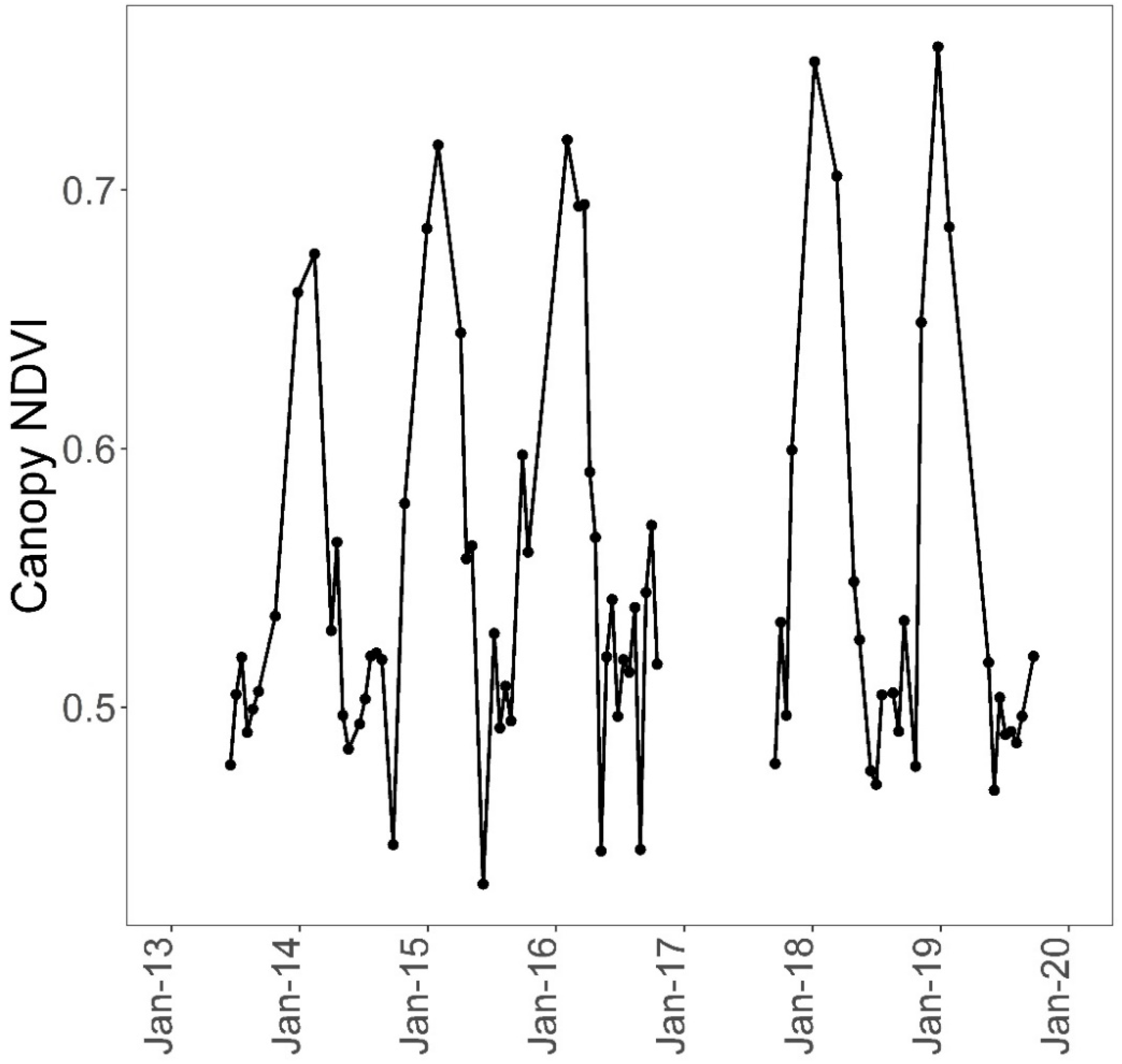
2.5. Canopy NDVI Retrieval Algorithm

While Equation (3) was used to test our classification approach, we ultimately aimed to partition Landsat 8 pixels with a mixture of different components to obtain the canopy NDVI of that pixel, which was retrieved using the following linear equation (Equation (4), derived from Equation (3)):

$${\mathrm{NDVI}}_{\mathrm{canopy}}=\left({\mathrm{NDVI}}_{\mathrm{P}}-{\mathrm{NDVI}}_{\mathrm{shade}}\times {\mathrm{F}}_{\mathrm{shade}}-{\mathrm{NDVI}}_{\mathrm{soil}}\times {\mathrm{F}}_{\mathrm{soil}}\right)/{\mathrm{F}}_{\mathrm{canopy}}$$

(4)

where ${\mathrm{F}}_{\mathrm{canopy}}+{\mathrm{F}}_{\mathrm{shade}}+{\mathrm{F}}_{\mathrm{soil}}=1$. Therefore, independent estimates of four unknowns were required in Equation (4): the NDVI values of the non-canopy components and two other components’ fractions. At the Yatir forest, the unknown NDVI_soil and NDVI_shade were accounted for based on the observed correlations with NDVI_canopy (Equations (5) and (6); Figure S1), which were derived from the UAV measurements:

$${\mathrm{NDVI}}_{\mathrm{shade}}=0.6\times {\mathrm{NDVI}}_{\mathrm{canopy}}+0.065$$

(5)

$${\mathrm{NDVI}}_{\mathrm{soil}}=0.85\times {\mathrm{NDVI}}_{\mathrm{canopy}}-0.16$$

(6)

The shade fraction was found to have a linear relationship with the sun elevation angle, whose slope and intercept are also related to the canopy fraction (Figure S2). Therefore, the shade fraction was estimated based on a function of the local sun elevation angle SA and the canopy fraction, as shown in Equation (7). Note that while in the Yatir forest, this correlation is expected to be nearly constant over time, this correlation may require updates in more dynamic forests:

$${\mathrm{F}}_{\mathrm{shade}}=\left(-0.0041\times {\mathrm{F}}_{\mathrm{canopy}}-0.3405\right)\times \mathrm{SA}+0.49\times {\mathrm{F}}_{\mathrm{canopy}}+30.45$$

(7)

Eventually, the soil fraction was simply the residue from the shade and canopy fractions (Equation (8)):

$${\mathrm{F}}_{\mathrm{soil}}=1-{\mathrm{F}}_{\mathrm{canopy}}-{\mathrm{F}}_{\mathrm{shade}}$$

(8)

Thus, by knowing the relevant canopy fraction and sun elevation angle, the canopy NDVI value could be back-calculated from the satellite NDVI.

3. Results

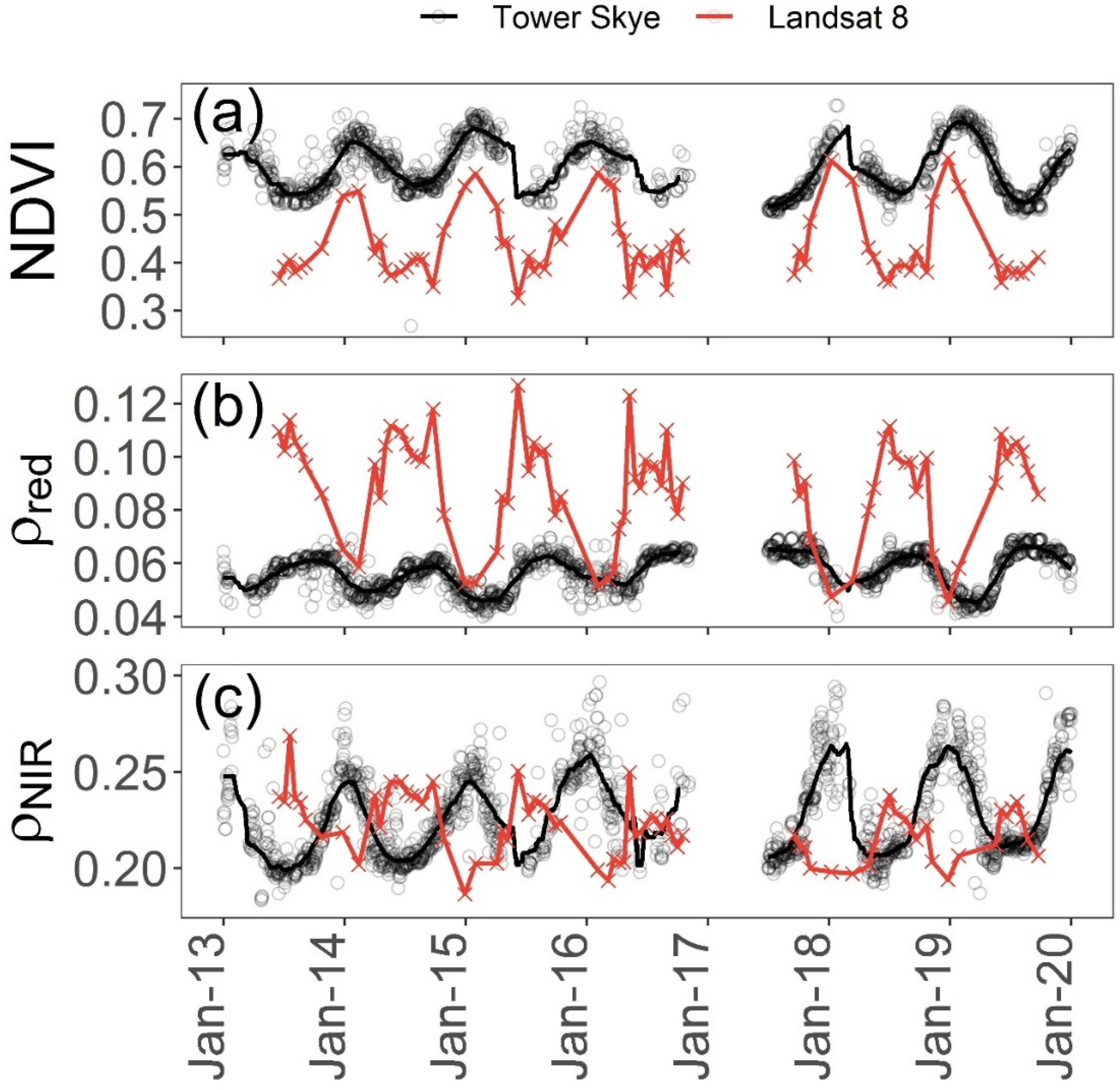
3.1. Comparison between Landsat 8 and Skye Data

A comparison of the NDVI values from the Landsat 8 surface product and tower-based Skye sensor at the Yatir flux tower showed similar changes over the six measurement years, with maximum values in February and minimum values in September (Figure 2a). However, an examination of the NDVI components indicated that while the red reflectance (ρ_red) showed agreement between the tower and satellite (Figure 2b), the NIR reflectance (ρ_NIR) had contrasting dynamics (Figure 2c). Moreover, large offsets were observed between the signals’ magnitudes in the two datasets, especially with ρ_red in the summer, which was two times higher in the tower data than in the satellite data.

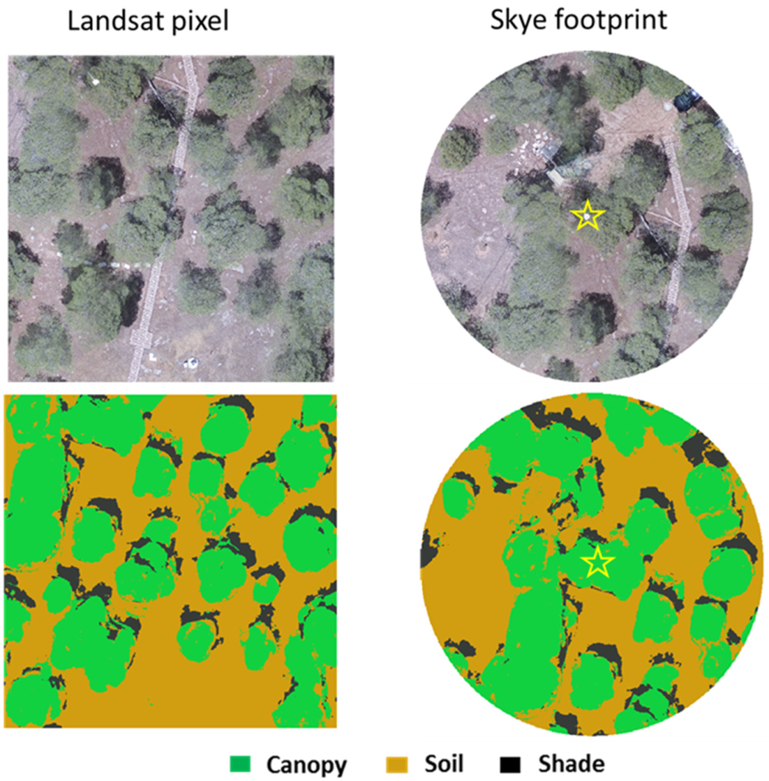
3.2. Image Classification of Canopy, Shade, and Soil

An example of the classification results for one Landsat 8 pixel (for 25 June 2019) and the parallel view of the Skye sensor were displayed and validated with the RGB map (Figure 3). The seven pixels around the flux tower (see yellow polygon in Figure 1c) were similarly used to analyze the surface component fractions and radiative properties. The temporal variations in the mean fraction of canopy, shaded soil, and exposed soil over the seven pixels, associated with the seasonal changes in solar angle, are presented in Figure 4. As expected, the mature evergreen study forest presented a near-constant canopy fraction (F_canopy, ~30%) throughout the study period. The shade fraction (F_shade) was high in the winter (up to 40%) and low in the summer (below 10%), which was consistent with seasonal changes in the sun elevation angle. The variation in the sunlit soil fraction showed an opposite pattern to that in the shaded one.

The Skye sensor was assumed to have a nadir view (as Landsat 8), with the classification method generating a canopy fraction of about 47% on its footprint. However, considering that the sensor’s position also resulted in a side view of the canopy, 3D simulations (see Methods) were also used. A canopy contribution of 95% was estimated, with combined signals from the exposed and shaded soil of about 5%, indicating the overriding role of the canopy in the tower-based sensor signals.

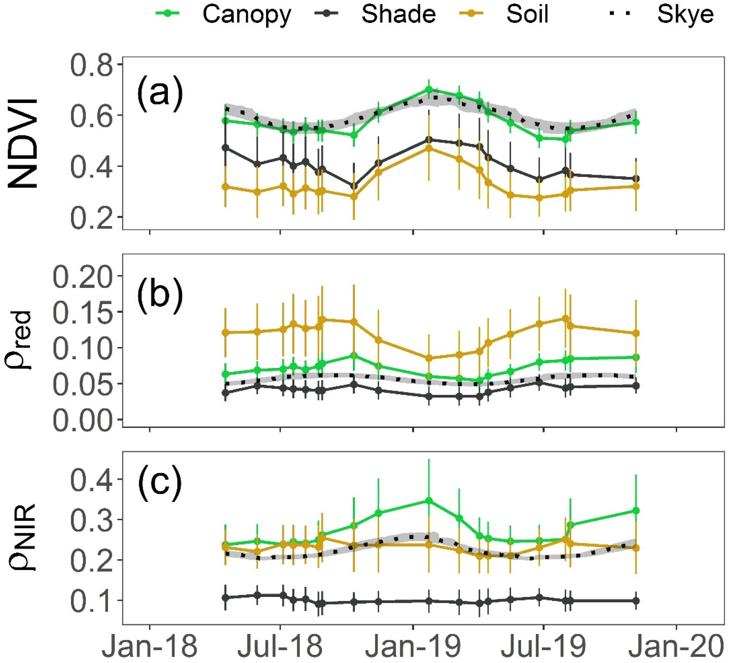
3.3. Radiative Properties of Canopy, Shade, and Soil

Seasonal variations in the reflectance and NDVI values of canopy, shade, and soil were analyzed (Figure 5). Despite different magnitudes of these values, similar dynamics were observed in the NDVI of these three components, with the maximum observed in February–March and the minimum observed in July–October. The canopy NDVI values were the highest, ranging from 0.55 to 0.70, while the soil NDVI values were the lowest, ranging from 0.3 to 0.5. The shade NDVI was intermediate between the canopy and soil. In the winter months, the shade and soil NDVI were more comparable. Similar to the NDVI, ρ_red also presented similar seasonal changes in the three components. Soil gave the highest ρ_red, with summer values (0.14, June–October) that were nearly two times those of the canopy (0.08). Shade presented the lowest ρ_red values, reflecting the strong absorption and reflection by the canopy. The patterns of NIR reflectance, ρ_NIR, however, were quite different (Figure 5c). The canopy and soil ρ_NIR values were similar in the summer months (about 0.25, July–September), followed by a sharp increase in the canopy values, which ended around February (0.35), compared to a mild decrease in the soil values, which lasted until the end of spring in April (0.22). The seasonal change in the shade ρ_NIR was nonsignificant. The variations in the canopy NDVI were close to those of the Skye NDVI. However, there was a clear offset in the reflectance values, with Skye showing lower values than those of the canopy, especially in ρ_NIR.

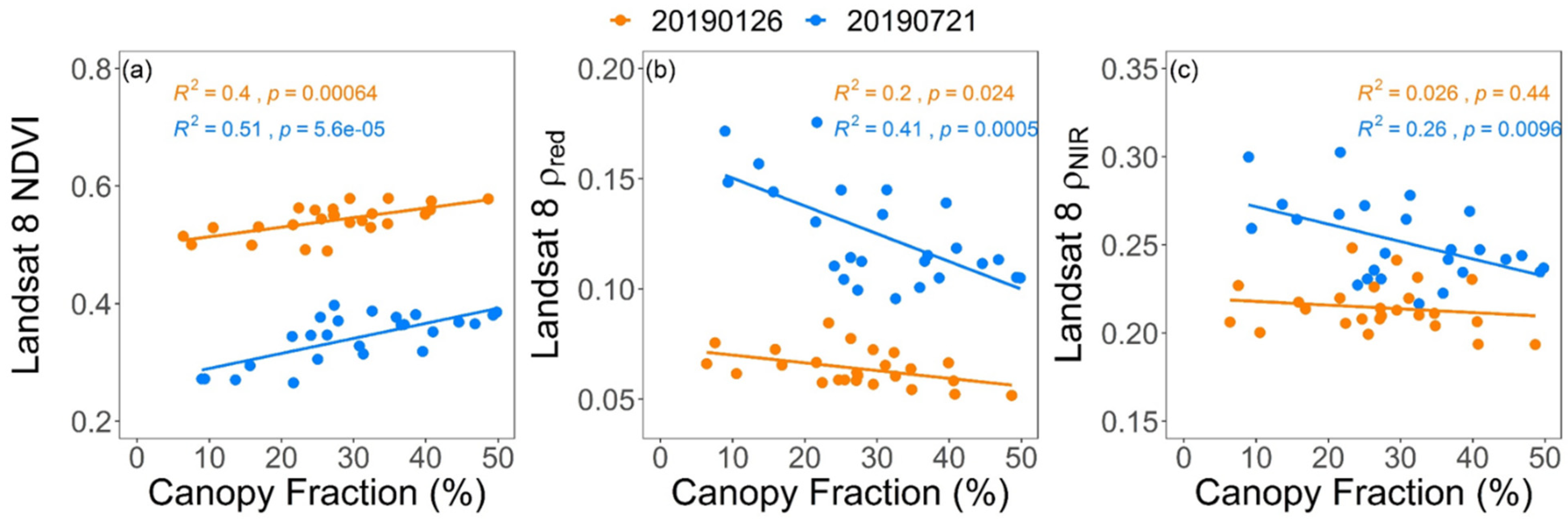
3.4. Reconstruction of Landsat 8 Data Using the UAV Results

Based on the UAV-measured fractions and reflectance values of the three components, attempts were made to reconstruct the satellite measurements. The reconstructed reflectance and NDVI values (NDVI_P-reconst) over the Landsat 8 pixels were generated using the linear equation that was provided as Equation (3). To validate the reconstructed values with the limited satellite data that were taken on different days, these pixels were assigned to the appropriate weeks of the year, and comparisons were made with data in the same week (Figure 6). The reconstructed NDVI (NDVI_P-reconst) was successfully validated, with an R² value of 0.94 and RMSE of 0.014 to the original Landsat 8 data. The reconstruction was also good for the ρ_red values but less accurate for ρ_NIR.

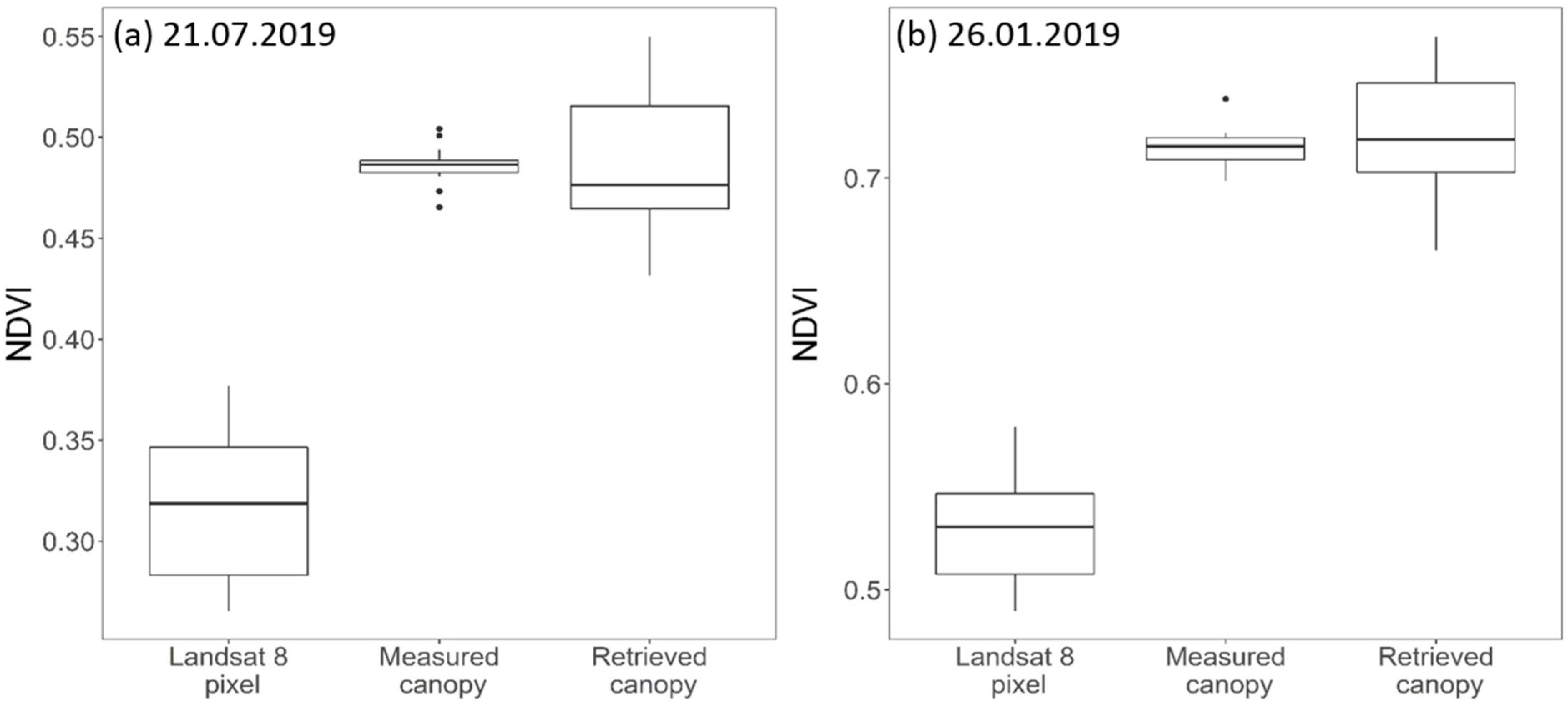
3.5. Retrieval of Canopy NDVI from Landsat 8 NDVI

The canopy NDVI retrieval algorithm was applied to 19 pixels outside the sampling area on two Landsat 8 imaging days in the summer (21 July 2019) and winter (26 January 2019). The canopy fraction was estimated from the UAV images on the neighboring days (31 July and 23 January 2019). The results were then validated with the UAV-measured canopy NDVI and compared with the Landsat 8 pixel NDVI values (Figure 7). The retrieved canopy NDVI values agreed well with the UAV-measured canopy values, with root mean square errors of 0.03 on both days. The canopy NDVI was about 0.48 in July and 0.72 in January, which represented a significant increase (July: 0.16, ~50%; January: 0.18, ~34%) compared to the original Landsat 8 NDVI.

This retrieval approach was also applied to the time series of the Landsat 8 NDVI for 2013–2019 as well (Figure 8). Notably, a constant canopy fraction of 30% was derived from the UAV measurements in 2018–2019, which was justified due to the slow growth of the mature semi-arid pine trees at the study site. The canopy NDVI showed prominent seasonal cycles, with peak values of up to 0.73 occurring in the winter season and low values of around 0.50 in the dry summer. An apparent trend of increases in the peak canopy NDVI over time was observed. This trend, however, is not sufficiently convincing due to the lack of Landsat 8 images on cloudy days, which happened frequently during the peak activity season.

The spatial variations in the Landsat 8 NDVI over all the 26 Landsat 8 pixels at the research site were directly related to variations in the canopy fraction across pixels (Figure 9). The correlation was slightly more significant in summer than in winter (with an R² of 0.51 and 0.40, respectively). The canopy fraction also showed a substantial relationship with Landsat 8 ρ_red, while lower correlations were found with ρ_NIR, especially in the winter.

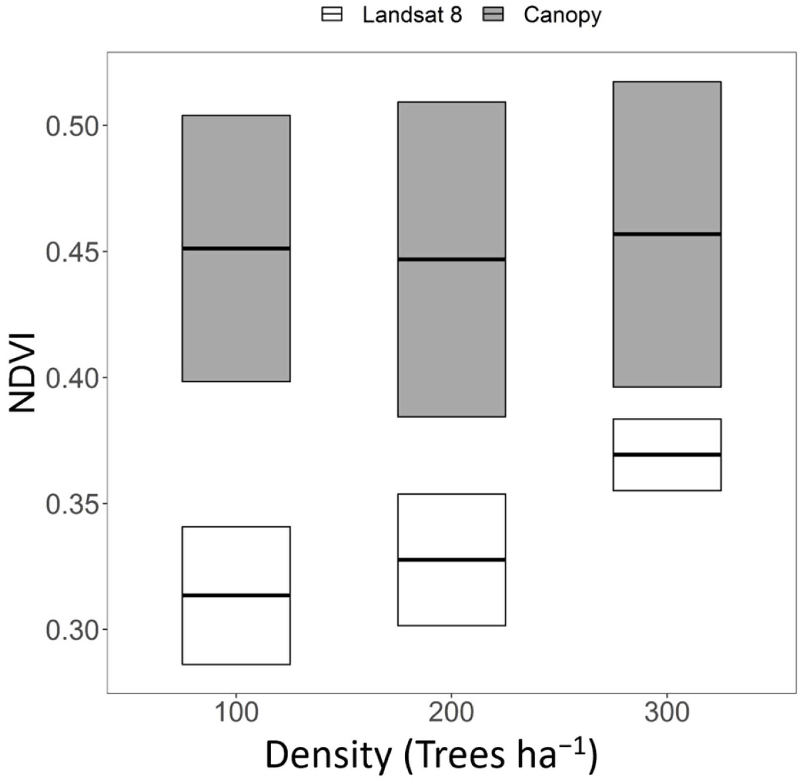
3.6. Stand Density Effect on Canopy NDVI

The effect of stand density on NDVI values was assessed in the Yatir thinning experimental site (Figure 10). The Landsat 8 surface NDVI on 6 August 2019, was extracted and averaged over pixels with the same densities. This image was chosen based on the availability of UAV flights on the next day (7 August 2019); these flights provided high-resolution canopy NDVI and fraction values. Note that the selected pixels were located within thinning plots where the tree density was controlled but not the tree distribution within the plot. The satellite pixels within the same density plot could have different numbers of trees and, in turn, yield different canopy fractions, which could add some variations to the results. Nevertheless, the results showed that the Landsat 8 NDVI increased with density, as expected. The Landsat 8 pixel NDVI for the 300 trees ha⁻¹ plot was about 0.05 higher than that for the 100 trees ha⁻¹ plot. At the same time, the canopy NDVI was essentially independent of the density effect and showed a constant value around 0.45.

4. Discussion

4.1. Radiative Properties of Canopy, Shaded, and Exposed Soil

Our study provides a relatively rare case (

Table 1. Overviews of NDVI values (ranges) of pine canopy, soil, and shade in recent studies.

Location	Surface Cover	Data Source	Ecosystem NDVI	Canopy NDVI	Soil NDVI	Shade NDVI
This study
Yatir, Israel	Aleppo pine	Landsat 8 surface product	0.4–0.6
LAI 1.7, 300/ha		UAV Multispectral images		0.55–0.7	0.3–0.5	0.35–0.5
		2013–2019
Vegetation
Hyytiälä, Finland [53]	Scots pine	Flux tower radiation sensors	0.5–0.75
LAI 3, 2500/ha		MODIS	0.1–0.8
		1997–2001
Puumala, Finland [54]	Scots pine (dominated)	Landsat 7	0.6–0.8
LAI 0.36–3.38	Norway Spruce	10 June 2000; 6 July 2001
Near Krasnoyarsk, Russia [55]	Scots pine	MODIS	0.1–0.8
600–800/ha		2003–2017
Codo site, Spain [56]	Oak (dominated)	UAV multispectral images		0.42
	Scots pine	26 November 2017
Soil
Global analysis [57]		AVHRR NDVI			0.05
		1992–1993
Global analysis [58]		AVHRR NDVI			0.03–0.05
		1981–2000
Global analysis [59]		Gutman and Ignatov (GI) model [60]			0.04
Worldwide samples [22]		Lab soil spectral data			0.2 ± 0.1
Shade
Taiwan [30]		ADS spectral images		0.64 sunlit canopy
Forests, plantation, grasslands		2007–2009		0.38 Shaded canopy
California, USA [43]		UAV optical images		0.88 sunlit canopy
Vineyard		Four campaigns in 2014–2016		0.82 shaded canopy

) outlining the detailed and long-term measurements of the distinct canopy and soil reflectance. Several studies in European ecosystems reported minor seasonal variations in pine forest NDVI values using flux tower-based radiation sensors or satellite measurements; however, these studies mainly focused on the ecosystem scale [53,54,55]. Other works have reported pure canopy NDVI from UAV multispectral images but only involved a single UAV campaign and could, therefore, not cover seasonal changes [56].

The spectrally distinct canopy signal showed, in contrast to the soil, a peak in ρ_red around October along with a prominent peak in ρ_NIR around January. The canopy reflectance in the red range was closely related to pigment content, as confirmed by the seasonal cycles in chlorophyll content, which reached the minimum around October and maximum around February and March [11]. The NIR reflectance at the study site was previously reported to be related to changes in the canopy structure, which could enhance or reduce the leaf light absorption [11]. The variations in soil reflectance at the study site, both in ρ_red and ρ_NIR, were inversely related to the seasonal variations in soil moisture, which were reported for this site previously [51]. This dependence of soil reflectance on the soil moisture level is consistent with previous publications [13,14,15].

The results showed a significant fraction of sunlit soil (60% in July and 30% in January) in the study area and a substantial seasonal variation in the soil NDVI, with a high value of 0.5 in the wet seasons. Despite its dark appearance, the shaded soil also had high NDVI values (0.35–0.5) and similar seasonal variations to the canopy and sunlit soil. As a result, the shaded areas also greatly influenced the measurements, especially in the sparse vegetation locations that introduced a high proportion of shaded soil (40% at Yatir forest in January). Such effects must be considered in soil spectral measurements in these sites. At the Yatir forest, we observed the lowest soil NDVI of 0.3 in the dry months which was much higher than the commonly used near-zero values. This result is more consistent with a study that reported high soil NDVI values with high spatial variability (0.2 ± 0.1) [22]. However, that study was based on soil spectral analysis in the lab, which may introduce significant uncertainties, in contrast to the in situ field results that were reported here. Notably, in previous studies, near-zero values were often used to represent soil NDVI [57,58,59,60], considering the annual lowest NDVI values within the satellite scene. These studies also often assumed that soil NDVI was spatially homogenous in the observation scene, which is not always justified. As shown in this study, several factors can influence the soil radiative properties, such as moisture and shading effects.

4.2. Canopy NDVI Retrieval Approach

Untangling these spectral and fractional effects of the main surface components in the study area allowed us to successfully reconstruct the mixed Landsat 8 signals from UAV measurements and validate them (Figure 6). Note that the reflectance values of each component were measured by the UAV multispectral camera, which has a NIR band that is centered at 790 nm, different from the satellite Landsat 8 and tower Skye sensor (both around 860 nm). While differences in the band settings could result in differences of up to 10% in the NDVI values of low NDVI surfaces [61], the effect is minimal in high NDVI vegetated areas [33] and allows the comparison between sensors with different band settings.

These results demonstrate the feasibility of retrieving canopy NDVI from satellite NDVI values and allowed us to simplify our canopy NDVI retrieval approach. These simplifications relied on the finding that the shade fraction can be estimated based on the sun angle and canopy fraction and that there are relatively robust relationships between the NDVI values of the canopy and the soil (Figures S1 and S2, Equations (5)–(7)). As a result, the key inputs that are required in this approach are the sun elevation and canopy fraction, which can often be estimated locally. When applied in more complex forests, other methodologies could be explored. The canopy fraction can be obtained via field measurements such as hemispherical photography and spherical densitometer [62,63]; empirical models using correlations between tree size parameters and canopy cover [64,65]; and remote sensing measurements using satellite, aerial, or UAV images [39,60,66,67]. Shaded area identification can be achieved using invariant color models [68], color identification on aerial RGB images [67], histogram thresholds in satellite images [69], or DSM analysis from hyperspectral and LiDAR data [70]. The NDVI values of other non-canopy components could be potentially replaced by satellite NDVI values of pixels containing a single component in the same area (e.g., soil pixel).

The results also highlight the potentially complicating effects of grass annuals in low-density ecosystems. We observed NDVI values of 0.5 and 0.4 for soil in winter with and without grass annuals, respectively. Note, however, that the arid and semi-arid grass annuals are usually short-lived (~3 months at the Yatir forest), with negligible signals for the rest of the year [71]. While this short-term signal can be partly avoided, further improvements are needed in the current methodology to address this issue in more detail.

Interestingly, a new NIRv index was recently introduced to better represent the vegetation in mixed-pixel scenes [21,28]. However, testing this approach using the Landsat 8 data in the study area indicated that this index failed under the sparse semi-arid conditions, such as in the Yatir forest (Figure S3). It is possible that under these conditions, the intense contributions of the low soil ρ_NIR overwhelmed the high ρ_NIR signals from trees in winter, thus reducing the forest NIRv signal to a comparable level to the surrounding desert. Therefore, using the NIRv approach could not substitute for the methodology that was developed here in these regions and ecosystem types.

4.3. Implications of the Retrieved Canopy NDVI

Our results demonstrated that spatial variations in low-resolution satellite NDVI do not necessarily indicate actual changes in canopy NDVI. Instead, these variations were induced by the combined effects of variations in canopy fraction and the complementary contributions of spectrally-distinct soil components. Indeed, a linear correlation between the Landsat 8 NDVI and canopy fraction across the forest was observed (Figure 9). This observation was further supported by the results from the Yatir thinning experiment that showed the canopy NDVI values to be similar across densities of between 100 and 300 trees ha⁻¹ (Figure 10). Notably, a recent study in the same thinning experiment indicated a large increase in the rates of leaf-scale photosynthesis in the lower branches of the trees in the 100 trees ha⁻¹ plot compared to that in the 300 trees ha⁻¹ plot due to higher PAR penetration [72]. Our results from the retrieval approach indicated that this effect may be limited only to the more impacted lower canopy layer and was not detected by the nadir-oriented top of canopy NDVI.

Despite being a mature evergreen forest and the homogenous spatial distribution of canopy NDVI, a pronounced seasonal signal was observed (Figure 8). The corrected canopy NDVI experienced a 50% increase in the canopy NDVI to peak values around February, compared with the minimum values in July that persisted throughout the dry summer until September. This is consistent with the increase of chlorophyll in the short active season [11]. The actual corrected Aleppo pine canopy NDVI values (0.50–0.73), irrespective of the low stand density, are also consistent with the NDVI values (0.50–0.75) of a dense temperate Scot pine forest [53], thus providing further confidence in the retrieval approach and its potential use in ecophysiological research.

5. Conclusions

In this study, we developed an approach to retrieve a corrected canopy (tree foliage) NDVI from the satellite data of mixed foliage and soil surfaces. The canopy NDVI retrieval approach assumed that the mixed NDVI is a simple combination of contributions from the main surface components (canopy foliage, exposed, and shaded soil surfaces). Thus, the canopy NDVI could be retrieved by independently characterizing the other elements’ fractional contribution, their reflectance properties (under the same conditions), and their seasonal dynamics. This was achieved with multiple high-resolution UAV campaigns over the study site. We concluded that the combined effects of these components explained the main apparent discrepancy between the satellite and tower-based NDVI estimates. Using the new derived canopy NDVI, we could show that the spatial variations in Landsat 8 NDVI data were due to variations in the stand density, with relatively small variations in the actual foliage NDVI values across the study site (as usually assumed by eddy covariance flux measurements at the forest center). These findings highlight the importance of accounting for non-vegetation contributions to low-resolution satellite measurements in low-density dry ecosystems.

References

1. Kerr, J.T.; Ostrovsky, M. From Space to Species: Ecological Applications for Remote Sensing. Trends Ecol. Evol. 2003, 18, 299–305. [Google Scholar] [CrossRef]
2. Xiao, J.; Chevallier, F.; Gomez, C.; Guanter, L.; Hicke, J.A.; Huete, A.R.; Ichii, K.; Ni, W.; Pang, Y.; Rahman, A.F.; et al. Remote Sensing of the Terrestrial Carbon Cycle: A Review of Advances over 50 Years. Remote Sens. Environ. 2019, 233, 111383. [Google Scholar] [CrossRef]
3. Lausch, A.; Erasmi, S.; King, D.; Magdon, P.; Heurich, M. Understanding Forest Health with Remote Sensing -Part I—A Review of Spectral Traits, Processes and Remote-Sensing Characteristics. Remote Sens. 2016, 8, 1029. [Google Scholar] [CrossRef] [Green Version]
4. Hall, F.G.; Shimabukuro, Y.E.; Huemmrich, K.F. Remote Sensing of Forest Biophysical Structure Using Mixture Decomposition and Geometric Reflectance Models. Ecol. Appl. 1995, 5, 993–1013. [Google Scholar] [CrossRef]
5. Xu, M.; Watanachaturaporn, P.; Varshney, P.K.; Arora, M.K. Decision Tree Regression for Soft Classification of Remote Sensing Data. Remote Sens. Environ. 2005, 97, 322–336. [Google Scholar] [CrossRef]
6. Chen, X.; Wang, D.; Chen, J.; Wang, C.; Shen, M. The Mixed Pixel Effect in Land Surface Phenology: A Simulation Study. Remote Sens. Environ. 2018, 211, 338–344. [Google Scholar] [CrossRef]
7. Smith, W.K.; Dannenberg, M.P.; Yan, D.; Herrmann, S.; Barnes, M.L.; Barron-Gafford, G.A.; Biederman, J.A.; Ferrenberg, S.; Fox, A.M.; Hudson, A.; et al. Remote Sensing of Dryland Ecosystem Structure and Function: Progress, Challenges, and Opportunities. Remote Sens. Environ. 2019, 233, 111401. [Google Scholar] [CrossRef]
8. Duman, T.; Huang, C.W.; Litvak, M.E. Recent Land Cover Changes in the Southwestern US Lead to an Increase in Surface Temperature. Agric. For. Meteorol. 2020, 297, 108246. [Google Scholar] [CrossRef]
9. Anderegg, W.R.L.; Anderegg, L.D.L.; Kerr, K.L.; Trugman, A.T. Widespread Drought-Induced Tree Mortality at Dry Range Edges Indicates That Climate Stress Exceeds Species’ Compensating Mechanisms. Glob. Chang. Biol. 2019, 25, 3793–3802. [Google Scholar] [CrossRef]
10. Allen, C.D.; Breshears, D.D.; McDowell, N.G. On Underestimation of Global Vulnerability to Tree Mortality and Forest Die-off from Hotter Drought in the Anthropocene. Ecosphere 2015, 6, 1–55. [Google Scholar] [CrossRef]
11. Wang, H.; Gitelson, A.; Sprintsin, M.; Rotenberg, E.; Yakir, D. Ecophysiological Adjustments of a Pine Forest to Enhance Early Spring Activity in Hot and Dry Climate. Environ. Res. Lett. 2020, 15, 114054. [Google Scholar] [CrossRef]
12. Musick, H.B.; Pelletier, R.E. Response to Soil Moisture of Spectral Indexes Derived from Bidirectional Reflectance in Thematic Mapper Wavebands. Remote Sens. Environ. 1988, 25, 167–184. [Google Scholar] [CrossRef]
13. Weidong, L.; Baret, F.; Xingfa, G.; Qingxi, T.; Lanfen, Z.; Bing, Z. Relating Soil Surface Moisture to Reflectance. Remote Sens. Environ. 2002, 81, 238–246. [Google Scholar] [CrossRef]
14. Lesaignoux, A.; Fabre, S.; Briottet, X. Influence of Soil Moisture Content on Spectral Reflectance of Bare Soils in the 0.4–14 Μm Domain. Int. J. Remote Sens. 2013, 34, 2268–2285. [Google Scholar] [CrossRef]
15. Lobell, D.B.; Asner, G.P. Moisture Effects on Soil Reflectance. Soil Sci. Soc. Am. J. 2002, 66, 722–727. [Google Scholar] [CrossRef]
16. Bedidi, A.; Cervelle, B.; Madeira, J.; Pouget, M. Moisture Effects on Visible Spectral Characteristics of Lateritic Soils. Soil Sci. 1992, 153, 129–141. [Google Scholar] [CrossRef]
17. Hoffer, R.M.; Johannsen, C.J. Ecological Potential in Spectral Signatures Analysis. Remote Sens. Ecol. 1969, 1–16. [Google Scholar]
18. Rouse, J.W., Jr.; Haas, R.H.; Schell, J.A.; Deering, D.W.; Rouse, J.W., Jr.; Haas, R.H.; Schell, J.A.; Deering, D.W. Monitoring Vegetation Systems in the Great Plains with Erts. NASA Spec. Publ. 1973, 351, 309. [Google Scholar]
19. Gamon, J.A.; Peñuelas, J.; Field, C.B. A Narrow-Waveband Spectral Index That Tracks Diurnal Changes in Photosynthetic Efficiency. Remote Sens. Environ. 1992, 41, 35–44. [Google Scholar] [CrossRef]
20. Gitelson, A.A. Wide Dynamic Range Vegetation Index for Remote Quantification of Biophysical Characteristics of Vegetation. J. Plant Physiol. 2004, 161, 165–173. [Google Scholar] [CrossRef] [Green Version]
21. Badgley, G.; Field, C.B.; Berry, J.A. Canopy Near-Infrared Reflectance and Terrestrial Photosynthesis. Sci. Adv. 2017, 3, e1602244. [Google Scholar] [CrossRef] [PubMed] [Green Version]
22. Montandon, L.M.; Small, E.E. The Impact of Soil Reflectance on the Quantification of the Green Vegetation Fraction from NDVI. Remote Sens. Environ. 2008, 112, 1835–1845. [Google Scholar] [CrossRef]
23. Chen, T.; de Jeu, R.A.M.; Liu, Y.Y.; van der Werf, G.R.; Dolman, A.J. Using Satellite Based Soil Moisture to Quantify the Water Driven Variability in NDVI: A Case Study over Mainland Australia. Remote Sens. Environ. 2014, 140, 330–338. [Google Scholar] [CrossRef]
24. Huete, A.R. A Soil-Adjusted Vegetation Index (SAVI). Remote Sens. Environ. 1988, 25, 295–309. [Google Scholar] [CrossRef]
25. Qi, J.; Chehbouni, A.; Huete, A.R.; Kerr, Y.H.; Sorooshian, S. A Modified Soil Adjusted Vegetation Index. Remote Sens. Environ. 1994, 126, 119–126. [Google Scholar] [CrossRef]
26. Rondeaux, G.; Steven, M.; Baret, F. Optimization of Soil-Adjusted Vegetation Indices. Remote Sens. Environ. 1996, 55, 95–107. [Google Scholar] [CrossRef]
27. Gilabert, M.A.; González-Piqueras, J.; García-Haro, F.J.; Meliá, J. A Generalized Soil-Adjusted Vegetation Index. Remote Sens. Environ. 2002, 82, 303–310. [Google Scholar] [CrossRef]
28. Baldocchi, D.D.; Ryu, Y.; Dechant, B.; Eichelmann, E.; Hemes, K.; Sanchez, C.R.; Shortt, R.; Szutu, D.; Valach, A.; Verfaillie, J.; et al. Outgoing Near Infrared Radiation from Vegetation Scales with Canopy Photosynthesis Across a Spectrum of Function, Structure, Physiological Capacity and Weather. J. Geophys. Res. Biogeosci. 2020, 125, e2019JG005534. [Google Scholar] [CrossRef]
29. Leblon, B.; Gallant, L.; Granberg, H. Effects of Shadowing Types on Ground-Measured Visible and near-Infrared Shadow Reflectances. Remote Sens. Environ. 1996, 58, 322–328. [Google Scholar] [CrossRef]
30. Hsieh, Y.T.; Wu, S.T.; Chen, C.T.; Chen, J.C. Analyzing Spectral Characteristics of Shadow Area from ADS-40 High Radiometric Resolution Aerial Images. Int. Arch. Photogramm. Remote Sens. Spat. Inf. Sci.-ISPRS Arch. 2016, 41, 223–227. [Google Scholar] [CrossRef] [Green Version]
31. Liu, W.; Yamazaki, F. Object-Based Shadow Extraction and Correction of High-Resolution Optical Satellite Images. IEEE J. Sel. Top. Appl. Earth Obs. Remote Sens. 2012, 5, 1296–1302. [Google Scholar] [CrossRef]
32. Hmimina, G.; Dufrêne, E.; Pontailler, J.Y.; Delpierre, N.; Aubinet, M.; Caquet, B.; de Grandcourt, A.; Burban, B.; Flechard, C.; Granier, A.; et al. Evaluation of the Potential of MODIS Satellite Data to Predict Vegetation Phenology in Different Biomes: An Investigation Using Ground-Based NDVI Measurements. Remote Sens. Environ. 2013, 132, 145–158. [Google Scholar] [CrossRef]
33. Ke, Y.; Im, J.; Lee, J.; Gong, H.; Ryu, Y. Characteristics of Landsat 8 OLI-Derived NDVI by Comparison with Multiple Satellite Sensors and in-Situ Observations. Remote Sens. Environ. 2015, 164, 298–313. [Google Scholar] [CrossRef]
34. Tittebrand, A.; Spank, U.; Bernhofer, C.H. Comparison of Satellite- and Ground-Based NDVI above Different Land-Use Types. Theor. Appl. Climatol. 2009, 98, 171–186. [Google Scholar] [CrossRef]
35. Jiang, Z.; Huete, A.R.; Chen, J.; Chen, Y.; Li, J.; Yan, G.; Zhang, X. Analysis of NDVI and Scaled Difference Vegetation Index Retrievals of Vegetation Fraction. Remote Sens. Environ. 2006, 101, 366–378. [Google Scholar] [CrossRef]
36. Hall, A.; Louis, J.; Lamb, D. Characterising and Mapping Vineyard Canopy Using High-Spatial- Resolution Aerial Multispectral Images. Comput. Geosci. 2003, 29, 813–822. [Google Scholar] [CrossRef]
37. Khokthong, W.; Zemp, D.C.; Irawan, B.; Sundawati, L.; Kreft, H.; Hölscher, D. Drone-Based Assessment of Canopy Cover for Analyzing Tree Mortality in an Oil Palm Agroforest. Front. For. Glob. Chang. 2019, 2, 12. [Google Scholar] [CrossRef] [Green Version]
38. Shin, P.; Sankey, T.; Moore, M.M.; Thode, A.E. Evaluating Unmanned Aerial Vehicle Images for Estimating Forest Canopy Fuels in a Ponderosa Pine Stand. Remote Sens. 2018, 10, 1266. [Google Scholar] [CrossRef] [Green Version]
39. Zhang, J.; Hu, J.; Lian, J.; Fan, Z.; Ouyang, X.; Ye, W. Seeing the Forest from Drones: Testing the Potential of Lightweight Drones as a Tool for Long-Term Forest Monitoring. Biol. Conserv. 2016, 198, 60–69. [Google Scholar] [CrossRef]
40. Torres-Sánchez, J.; Peña, J.M.; de Castro, A.I.; López-Granados, F. Multi-Temporal Mapping of the Vegetation Fraction in Early-Season Wheat Fields Using Images from UAV. Comput. Electron. Agric. 2014, 103, 104–113. [Google Scholar] [CrossRef]
41. Cai, D.; Li, M.; Bao, Z.; Chen, Z.; Wei, W.; Zhang, H. Study on Shadow Detection Method on High Resolution Remote Sensing Image Based on HIS Space Transformation and NDVI Index. In Proceedings of the 2010 18th International Conference on Geoinformatics, Beijing, China, 18–20 June 2010. [Google Scholar] [CrossRef]
42. Qiao, X.; Yuan, D.; Li, H. Urban Shadow Detection and Classification Using Hyperspectral Image. J. Indian Soc. Remote Sens. 2017, 45, 945–952. [Google Scholar] [CrossRef]
43. Aboutalebi, M.; Torres-Rua, A.F.; Kustas, W.P.; Nieto, H.; Coopmans, C.; McKee, M. Assessment of Different Methods for Shadow Detection in High-Resolution Optical Imagery and Evaluation of Shadow Impact on Calculation of NDVI, and Evapotranspiration. Irrig. Sci. 2019, 37, 407–429. [Google Scholar] [CrossRef]
44. Bhatnagar, S.; Gill, L.; Ghosh, B. Drone Image Segmentation Using Machine and Deep Learning for Mapping Raised Bog Vegetation Communities. Remote Sens. 2020, 12, 2602. [Google Scholar] [CrossRef]
45. Cunliffe, A.M.; Brazier, R.E.; Anderson, K. Ultra-Fine Grain Landscape-Scale Quantification of Dryland Vegetation Structure with Drone-Acquired Structure-from-Motion Photogrammetry. Remote Sens. Environ. 2016, 183, 129–143. [Google Scholar] [CrossRef] [Green Version]
46. Zhu, Z.; Woodcock, C.E. Object-Based Cloud and Cloud Shadow Detection in Landsat Imagery. Remote Sens. Environ. 2012, 118, 83–94. [Google Scholar] [CrossRef]
47. Sona, G.; Passoni, D.; Pinto, L.; Pagliari, D.; Masseroni, D.; Ortuani, B.; Facchi, A. UAV Multispectral Survey to Map Soil and Crop for Precision Farming Applications. ISPRS-Int. Arch. Photogramm. Remote Sens. Spat. Inf. Sci. 2016, 41, 1023–1029. [Google Scholar] [CrossRef] [Green Version]
48. Bastin, J.F.; Berrahmouni, N.; Grainger, A.; Maniatis, D.; Mollicone, D.; Moore, R.; Patriarca, C.; Picard, N.; Sparrow, B.; Abraham, E.M.; et al. The Extent of Forest in Dryland Biomes. Science 2017, 356, 635–638. [Google Scholar] [CrossRef] [PubMed] [Green Version]
49. Tatarinov, F.; Rotenberg, E.; Maseyk, K.; Ogée, J.; Klein, T.; Yakir, D. Resilience to Seasonal Heat Wave Episodes in a Mediterranean Pine Forest. New Phytol. 2016, 210, 485–496. [Google Scholar] [CrossRef] [Green Version]
50. Qubaja, R.; Grünzweig, J.M.; Rotenberg, E.; Yakir, D. Evidence for Large Carbon Sink and Long Residence Time in Semiarid Forests Based on 15 Year Flux and Inventory Records. Glob. Chang. Biol. 2020, 26, 1626–1637. [Google Scholar] [CrossRef]
51. Preisler, Y.; Tatarinov, F.; Grünzweig, J.M.; Bert, D.; Ogée, J.; Wingate, L.; Rotenberg, E.; Rohatyn, S.; Her, N.; Moshe, I.; et al. Mortality versus Survival in Drought-affected Aleppo Pine Forest Depends on the Extent of Rock Cover and Soil Stoniness. Funct. Ecol. 2019, 33, 901–912. [Google Scholar] [CrossRef]
52. Dan, J.; Koyumdjisky, H. The Soils of Israel and Their Distribution. J. Soil Sci. 1963, 14, 12–20. [Google Scholar] [CrossRef]
53. Wang, Q.; Tenhunen, J.; Dinh, N.Q.; Reichstein, M.; Vesala, T.; Keronen, P. Similarities in Ground- and Satellite-Based NDVI Time Series and Their Relationship to Physiological Activity of a Scots Pine Forest in Finland. Remote Sens. Environ. 2004, 93, 225–237. [Google Scholar] [CrossRef]
54. Stenberg, P.; Rautiainen, M.; Manninen, T.; Voipio, P.; Smolander, H. Reduced Simple Ratio Better than NDVI for Estimating LAI in Finnish Pine and Spruce Stands. Silva Fenn. 2004, 38, 3–14. [Google Scholar] [CrossRef] [Green Version]
55. Ivanova, Y.; Kovalev, A.; Soukhovolsky, V. Modeling the Radial Stem Growth of the Pine (Pinus sylvestris L.) Forests Using the Satellite-Derived Ndvi and Lst (Modis/Aqua) Data. Atmosphere 2021, 12, 12. [Google Scholar] [CrossRef]
56. Cardil, A.; Otsu, K.; Pla, M.; Silva, C.A.; Brotons, L. Quantifying Pine Processionary Moth Defoliation in a Pine-Oak Mixed Forest Using Unmanned Aerial Systems and Multispectral Imagery. PLoS ONE 2019, 14, e0213027. [Google Scholar] [CrossRef]
57. Zeng, X.; Dickinson, R.E.; Walker, A.; Shaikh, M.; Defries, R.S.; Qi, J. Derivation and Evaluation of Global 1-Km Fractional Vegetation Cover Data for Land Modeling. J. Appl. Meteorol. 2000, 39, 826–839. [Google Scholar] [CrossRef]
58. Matsui, T.; Lakshmi, V.; Small, E.E. The Effects of Satellite-Derived Vegetation Cover Variability on Simulated Land-Atmosphere Interactions in the NAMS. J. Clim. 2005, 18, 21–40. [Google Scholar] [CrossRef]
59. Gan, T.Y.; Burges, S.J. Assessment of Soil-Based and Calibrated Parameters of the Sacramento Model and Parameter Transferability. J. Hydrol. 2006, 320, 117–131. [Google Scholar] [CrossRef]
60. Gutman, G.; Ignatov, A. The Derivation of the Green Vegetation Fraction from NOAA/AVHRR Data for Use in Numerical Weather Prediction Models. Int. J. Remote Sens. 1998, 19, 1533–1543. [Google Scholar] [CrossRef]
61. Teillet, P.M.; Ren, X. Spectral Band Difference Effects on Vegetation Indices Derived from Multiple Satellite Sensor Data. Can. J. Remote Sens. 2008, 34, 159–173. [Google Scholar] [CrossRef]
62. Evans, A.G.C.; Coombe, D.E. Hemisperical and Woodland Canopy Photography and the Light Climate. J. Ecol. 1959, 47, 103–113. [Google Scholar] [CrossRef]
63. Lemmon, P.E. A Spherical Densiometer for Estimating Forest Overstory Density. For. Sci. 1956, 2, 314–320. [Google Scholar] [CrossRef]
64. Fiala, A.C.S.; Garman, S.L.; Gray, A.N. Comparison of Five Canopy Cover Estimation Techniques in the Western Oregon Cascades. For. Ecol. Manag. 2006, 232, 188–197. [Google Scholar] [CrossRef]
65. Korhonen, L.; Korhonen, K.T.; Rautiainen, M.; Stenberg, P. Estimation of Forest Canopy Cover: A Comparison of Field Measurement Techniques. Silva Fenn. 2006, 40, 577–588. [Google Scholar] [CrossRef] [Green Version]
66. Gitelson, A.A.; Kaufman, Y.J.; Stark, R.; Rundquist, D. Novel Algorithms for Remote Estimation of Vegetation Fraction. Remote Sens. Environ. 2002, 80, 76–87. [Google Scholar] [CrossRef] [Green Version]
67. Poblete-Echeverría, C.; Olmedo, G.F.; Ingram, B.; Bardeen, M. Detection and Segmentation of Vine Canopy in Ultra-High Spatial Resolution RGB Imagery Obtained from Unmanned Aerial Vehicle (UAV): A Case Study in a Commercial Vineyard. Remote Sens. 2017, 9, 268. [Google Scholar] [CrossRef] [Green Version]
68. Salvador, E.; Cavallaro, A.; Ebrahimi, T. Shadow Identification and Classification Using Invariant Color Models. In Proceedings of the 2001 IEEE International Conference on Acoustics, Speech, and Signal Processing, Proceedings (Cat. No.01CH37221), Salt Lake City, UT, USA, 7–11 May 2001; Volume 3, pp. 1545–1548. [Google Scholar]
69. Dare, P.M. Shadow Analysis in High-Resolution Satellite Imagery of Urban Areas. Photogramm. Eng. Remote Sens. 2005, 71, 169–177. [Google Scholar] [CrossRef] [Green Version]
70. Tolt, G.; Shimoni, M.; Ahlberg, J. A Shadow Detection Method for Remote Sensing Images Using VHR Hyperspectral and LIDAR Data. In Proceedings of the 2011 IEEE International Geoscience and Remote Sensing Symposium, Vancouver, BC, Canada, 24–29 July 2011; pp. 4423–4426. [Google Scholar]
71. Karnieli, A. Natural Vegetation Phenology Assessment by Ground Spectral Measurements in Two Semi-Arid Environments. Int. J. Biometeorol. 2003, 47, 179–187. [Google Scholar] [CrossRef]
72. Tsamir, M.; Gottlieb, S.; Preisler, Y.; Rotenberg, E.; Tatarinov, F.; Yakir, D.; Tague, C.; Klein, T. Stand Density Effects on Carbon and Water Fluxes in a Semi-Arid Forest, from Leaf to Stand-Scale. For. Ecol. Manag. 2019, 453, 117573. [Google Scholar] [CrossRef]
Figure 1. (a) The location of the Yatir forest between the Mediterranean Sea and the Dead Sea in southern Israel. (b) The Yatir flux tower site and thinning experimental plots in UTM zone 36R. (c) The Yatir tower area on the UAV RGB image for 31 July 2019. The circle represents the tower Skye radiometer footprint (15 m radius). The squares represent the Landsat 8 pixels (30 × 30 m; 26 pixels), based on their center coordinates that were extracted from the georeferenced Landsat 8 images. The pixels inside the yellow polygon were used to compare Landsat 8 and tower Skye and analyze the fractional contributions of canopy, soil, and shade. The pixels outside the polygon were used to validate the canopy NDVI retrieval approach. (d) Landsat 8 pixels in the thinning plots, with numbers indicating stand densities of 100, 200, and 300 trees per hectare.
Remotesensing 14 03681 g001
Figure 2. Comparisons of Landsat 8 surface (red) and tower-based radiometer Skye data (black) over a similar sensing area for the period of 2013–2019: (a) NDVI; (b) red reflectance; (c) NIR reflectance. Crosses indicate Landsat 8 data on a 16-day revisit cycle that were filtered for cloud cover below 10%. The open circles indicate daily Skye measurements that were averaged over 9:45–11:15 local time, and the black lines represent the 90-day moving average.
Remotesensing 14 03681 g002
Figure 3. An example of image classification using UAV multispectral images at 13:00 local time on 25 June 2019, compared with the RGB image. The left column shows the Landsat 8 pixel (30 × 30 m2). The right column shows the Skye footprint area, with a radius of 15 m, and the star indicates the sensor location. Canopy, shade, and soil are shown in green, black, and brown, respectively.
Remotesensing 14 03681 g003
Figure 4. Variations in the fraction of canopy, exposed, and shaded soil in the tower area are presented in green, black, and brown, respectively. Symbols with different colors on the same date are fractions that were calculated from the same UAV flight with sums equal to 100%.
Remotesensing 14 03681 g004
Figure 5. The UAV-measured (a) NDVI, (b) red reflectance, and (c) NIR reflectance for pure canopy (in green), bare soil (in brown), and shade (in black) from April 2018 to May 2019. The dots are the mean values over the Landsat 8 tower pixels for each UAV flight, with the error bars indicating the standard deviations in the pixel area. The dotted line represents the mean seasonal variations of the Skye data in 2013–2018 based on a 90-day moving average of the raw measurements. The grey area presents the standard deviations of the multi-year seasonal variations.
Remotesensing 14 03681 g005
Figure 6. The correlations between Landsat 8 and UAV-reconstructed (a) NDVI, (b) red reflectance, and (c) NIR reflectance over the same Landsat 8 pixels. The UAV-reconstructed data were calculated using the linear correlation (Equation (3)) and the UAV-measured fractions and reflectance values. The dots represent the UAV and Landsat 8 data for the same week. The black line indicates the linear regression of the correlation, and the red dashed line is the 1:1 line.
Remotesensing 14 03681 g006
Figure 7. Boxplots of satellite Landsat 8 pixel NDVI (original and retrieved) and directly measured canopy NDVI over 19 pixels around the tower (see Figure 1) on a summer day ((a) 12 July 2019) and a winter day ((b) 26 January 2019). The measured canopy NDVI is based on the high-resolution (5 cm) UAV measurements, and the Landsat 8-retrieved canopy NDVI is based on our retrieval algorithm. The root mean square error between the measured and retrieved canopy NDVI was 0.03 in both seasons.
Remotesensing 14 03681 g007
Figure 8. Time series of canopy NDVI that was retrieved from Landsat 8 NDVI for 2013–2019. Each data point refers to the canopy NDVI on a Landsat 8 imaging day.
Remotesensing 14 03681 g008
Figure 9. Correlations of canopy fraction with Landsat 8 data of (a) NDVI, (b) red reflectance, and (c) NIR reflectance. Each data point represents one Landsat 8 pixel in the tower area. The satellite data were taken on two Landsat 8 imaging days (21 July and 26 January 2019). The canopy fractions were calculated from two UAV flights on 31 July and 23 January 2019.
Remotesensing 14 03681 g009
Figure 10. Retrieved Canopy NDVI (in grey) and Landsat 8 NDVI (in white) for the Yatir thinning experimental site with stand densities of 100, 200, and 300 trees ha−1 using images that were taken on 6 August 2019. The horizontal line in each box represents the mean value, and the box boundaries indicate the range.
Remotesensing 14 03681 g010