Translational Compensation Algorithm for Ballistic Targets in Midcourse Based on Template Matching

Abstract

The high-speed movement of a ballistic target will cause folding and translation of the micro-Doppler, which will affect the extraction of micro-motion features. To address the adverse effects of high-speed movement of ballistic targets in midcourse on the extraction of micro-motion features, a novel translational compensation algorithm based on template matching is proposed. Firstly, a 512 × 512 time-frequency map is obtained by binarization and down-sampling. The matching template then convolves the time-frequency map to obtain contour-like points. Then, the upper and lower contour points are preliminarily determined by the extreme value, and all actual contour points are screened out through structural similarity. Lastly, the upper and lower trend lines are determined and translation parameters for compensation by polynomial fitting are estimated. Simulation results show that the proposed algorithm has lower requirements for time-frequency resolution, higher precision and lower time complexity as a whole. Furthermore, it is also applicable to spectral aliasing.

1. Introduction

The midcourse of ballistic missiles is often accompanied by the release of decoys, which makes it difficult to detect radar targets. Traditional recognition methods based on target characteristics have difficulty distinguishing warheads from decoys. It is necessary to improve the accuracy of target recognition using target micro-motion information [1]. Chen V C divides target micro-movement into rotation, conical rotation, swing and other forms [2,3]. Most existing micro-motion feature extraction and characterisation research methods are designed solely for micro-motion. However, translation and micro-motion occur during flight of the ballistic target. Translation can destroy the structure of the micro-Doppler and cause it to tilt, fold or translate. Therefore, translational compensation is required before the micro-Doppler characteristics of ballistic targets are investigated.

Researchers have proposed a variety of methods to address the problem of target translation compensation in the middle of the ballistic object trajectory. They can mainly be divided into translation compensation methods based on the Doppler spectrum information [4,5], methods based on signal processing [6,7,8,9], methods based on time-frequency analysis [10,11,12,13,14] and other types of method [15,16,17,18,19,20].

The translation compensation method based on Doppler spectrum information mainly uses the echo spectrum to estimate the speed and acceleration of the target through correlation transformation and related information, to achieve target translation compensation. Target translation compensation methods include the spectral rearrangement method and the template method. The spectral rearrangement method detects the spectral peaks of each pulse. Then, the peaks and their corresponding signal spectral regions are centered to achieve translation compensation [4]. The template method compensates for the echo signal using the known velocity and acceleration in the template database. Then, it calculates the relevant evaluation index of the compensated signal spectrum. The template data corresponding to the optimal value of the evaluation index are the speed and acceleration of the target [5].

The translation compensation method based on signal processing uses digital signal processing technology to simplify the echo form or reduce the dimension of echo parameters. Then, it estimates the target translation parameters to achieve compensation through related technical methods. This type of method has a significant inhibitory effect on the target fretting component. At present, such target translation compensation methods primarily include conjugate multiplication and the state-space method. Conjugate multiplication is divided into two types: delayed conjugate multiplication and symmetric conjugate multiplication. Multiplication of the delayed signal and the conjugate signal or multiplication of the symmetrical delayed signal is used to reduce the target translation order. Then, the translation parameters are estimated step-by-step by combining Radon transform, fractional Fourier transform, spectral peak search and other methods [6,7,8]. The state-space method derives the relationship between the cross-correlation function of the normalized sampling sequence of two adjacent pulse echoes and the radial velocity of the target to obtain the estimation formula of the radial velocity of the target. Therefore, the speed of the target can be estimated indirectly by straightforward measurement [9].

The translation compensation method based on time-frequency analysis is mainly aimed at echo time-frequency data and can be combined with the image processing method to estimate the target translation parameters and achieve target translation compensation. At present, such target translation compensation methods include the (extended) Hough/Radon transform method, the corner detection method and the entropy value method. The (extended) Hough/Radon transform method uses the time-frequency analysis method to transform time-domain echo data into the time-frequency domain. Then, it uses the (extended) Hough/Radon transform to project the implicit features in the time-frequency domain to the dominant features in the parameter domain. The peak detection method entails the detection of dominant features to better estimate the target translation parameters [10,11]. This method can achieve parameter dimensionality reduction, but the time complexity increases sharply with increase in parameter quantity. The corner detection method detects the corner points of the time-frequency diagram to obtain the intersection points that reflect the movement trajectory of the target. Then, the translation parameters are estimated by combining the fitting methods [12,13]. This method is dependent on the time-frequency transform method and requires extremely high time-frequency resolution. The entropy method uses the information entropy of the time-frequency map, after compensation with different parameters, to judge the compensation effect and achieve high-precision translation compensation of the target [14]. The entropy method has extremely high requirements on the quality of the time-frequency map. More importantly, the noise suppresses the compensation effect significantly, and the computation time increases rapidly with increase in the time-frequency graph scale. In addition to the above shortcomings, most translation compensation methods based on time-frequency analysis are completely ineffective for spectral aliasing.

To address the shortcomings of the translation compensation method based on time-frequency analysis, this paper proposes a translation compensation method based on template matching. The method involves first obtaining a binary image through Gaussian filtering and binarization. Next, according to the characteristics of the micro-Doppler curve, a matching template is designed and convolution matching performed with the binary image to obtain all the contour points of the overall micro-Doppler curve. Then, the upper and lower contour points are preliminarily determined by the maximum and minimum values. Meanwhile, the structural similarity in the image processing field is used to judge the authenticity of the contour points and eliminate all the false contour points. Finally, a polynomial fitting method is used to fit the upper and lower trend lines. The average value is taken to estimate the translational parameters of the target and to achieve compensation for the translation.

In summary, the proposed algorithm provides a matching template construction method for contour points suitable for motion compensation. Combined with the structural similarity in image processing technology, the precise detection of external contour points, reflecting the translational trend in the time-frequency diagram, is achieved. The algorithm offers a new approach to the translational compensation of ballistic midcourse targets. In addition, the adaptive aliasing judgment and the order of translational fit make practical application of the algorithm possible.

This paper is organized as follows: In Section 2, the motion model and echo model of the target in the middle trajectory are described. Section 3 presents the theory underpinning the proposed algorithm and its key steps. In Section 4, the simulations performed are discussed. Section 5 provides the conclusions.

2. Target Motion Model in the Middle of the Trajectory

Assuming that the target in the middle of the ballistic trajectory is a cone, its precession model is shown in Figure 1. The center of gravity of the target is the origin, the precession axis is the z axis. The y axis is located in the plane formed by the precession axis and the target symmetry axis (i.e., the spin axis). The x axis satisfies the right-handed spiral theorem to construct a rectangular coordinate system. The distance from the top of the cone A to the gravity is $h_1$, the distance from the bottom of the cone to the gravity is $h_2$, the radius of the bottom surface is r, the angle between the target precession axis and the spin axis is $\theta$ (that is, the precession angle). The precession angular velocity is ${\omega }_c$. The spin angular velocity is ${\omega }_s$. The angle between the radar line of sight (LOS) and the spin axis is $\beta$, the azimuth angle is $\phi$, and the pitch angle is $\alpha$.

It can be seen from [21] that when electromagnetic waves are incident at any angle, there are only three points on the cone target, namely, one at the top of the cone (point A in Figure 1) and two at the edge of the bottom surface (B and C in Figure 1). The bottom edge scattering point is generally the intersection of the plane formed by the incident ray and the axis of symmetry and the bottom edge of the cone. Therefore, the micro-Doppler formula of the above three scattering points can be obtained without considering the occlusion effect.

$$\left\{\begin{array}{c}{f}_{Ad}=\frac{2}{\lambda }{\omega }_c{h}_{1}sin\theta sin\alpha cos({\omega }_{c}t+{\phi }_0)\hfill \\ f_{Bd}=\frac{2}{\lambda }\left[h_2+r\frac{F\left(t\right)}{\sqrt{1-F^2\left(t\right)}}\right]{\omega }_{c}sin\theta cos\alpha cos({\omega }_{c}t+{\phi }_0)\hfill \\ f_{Cd}=\frac{2}{\lambda }\left[h_2-r\frac{F\left(t\right)}{\sqrt{1-F^2\left(t\right)}}\right]{\omega }_{c}sin\theta cos\alpha cos({\omega }_{c}t+{\phi }_0)\hfill \end{array}\right.$$

(1)

Among the terms, $F\left(t\right)=sin\theta sin\alpha sin({\omega }_{c}t+{\phi }_0)+cos\theta cos\alpha$, $\lambda$ is the signal wavelength and ${\phi }_0$ is the initial azimuth.

Then, the radial distance caused by the micro-motion of the target is

$$r_{im}\left(t\right)=\frac{\lambda }{2}\int f_{id}dt,i=A,B,C.$$

(2)

where $r_{im}\left(t\right)$ represents the real-time radial distance of point i caused by fretting, and $f_{id}$ represents the micro-Doppler of point i.

Assuming that a single-frequency signal is transmitted, the radar baseband echo signal $s\left(t\right)$ at this time is

$$s\left(t\right)=\sum _{i}exp\left\{-j\frac{4\pi }{\lambda }{r}_{im}\left(t\right)\right\},i=A,B,C.$$

(3)

The Doppler will be severely folded when the target is flying at a high speed. In the middle of the trajectory, the target flight trajectory is relatively stable and the radar is in a tracking state. The echo can be roughly compensated with the speed measured by the radar at a certain pulse. The translational trajectory of the target after rough compensation is

$$r_T\left(t\right)=r_0+vt+a_1{t}^2+a_2{t}^3.$$

(4)

where $r_T\left(t\right)$ is the radial distance caused by translation, $r_0$ is the initial distance, v is the residual velocity after coarse compensation, and $a_1,a_2$ are the first-order acceleration and the second-order acceleration, respectively. Then the radial distance of the target relative to the radar at this time is $R_i\left(t\right)$.

$$R_i\left(t\right)=r_T\left(t\right)+r_{im}\left(t\right)=r_0+vt+a_1{t}^2+a_2{t}^3+\frac{\lambda }{2}\int f_{id}dt.$$

(5)

According to Formula (5), the baseband echo signal of the target is obtained as

$$s\left(t\right)=\sum _{i}exp\left\{-j\frac{4\pi }{\lambda }{R}_i\left(t\right)\right\},i=A,B,C.$$

(6)

The target micro-Doppler is

$$f_{md}=\frac{1}{2\pi }\frac{d\varphi }{dt}=-\sum _i\left(f_{id}+\frac{2}{\lambda }\frac{d{R}_i\left(t\right)}{dt}\right)=\sum _i\left[f_{id}+\frac{2}{\lambda }(v+2a_{1}t+3a_2{t}^2)\right],i=A,B,C.$$

(7)

3. Target Translation Compensation Based on Template Matching

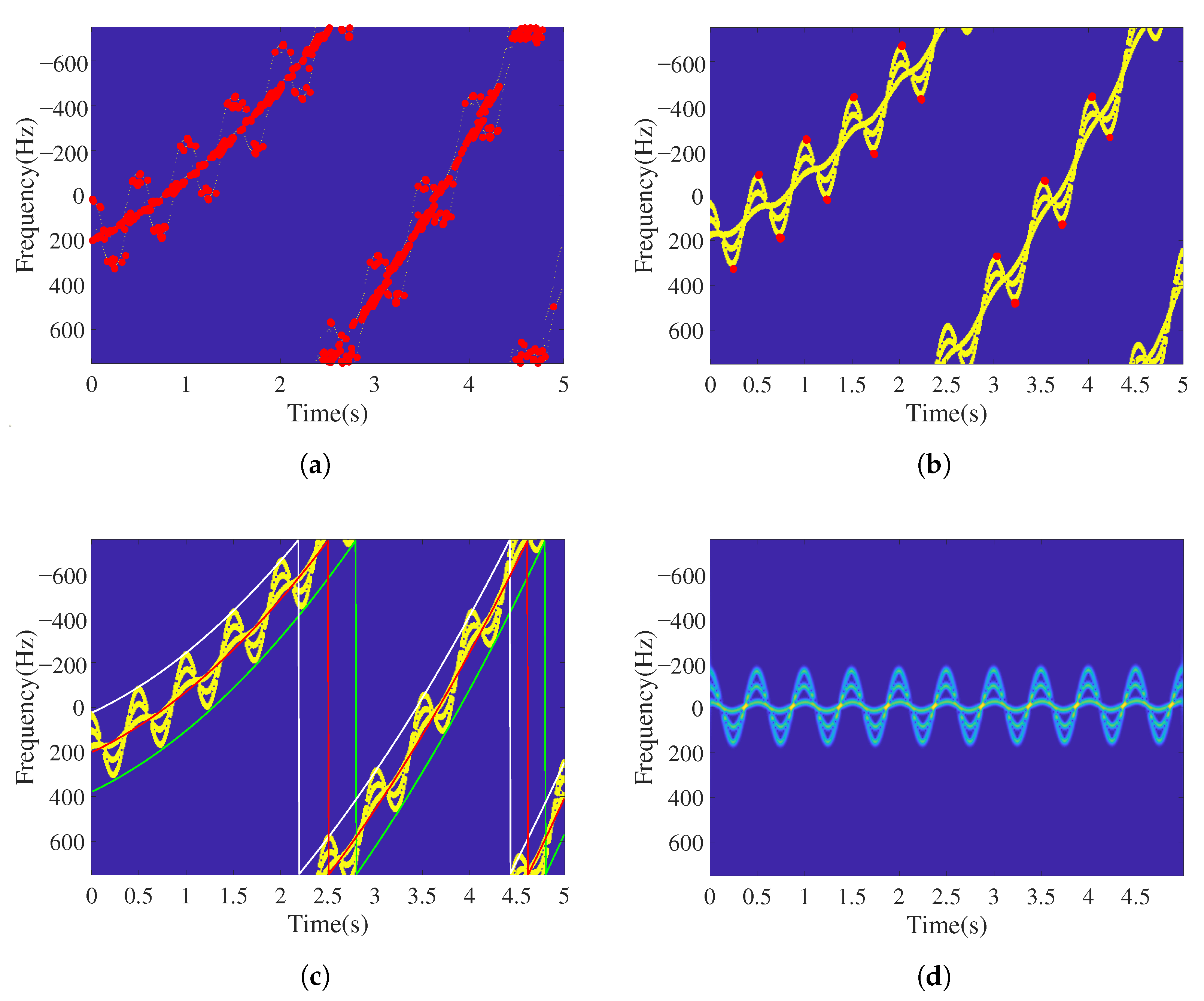
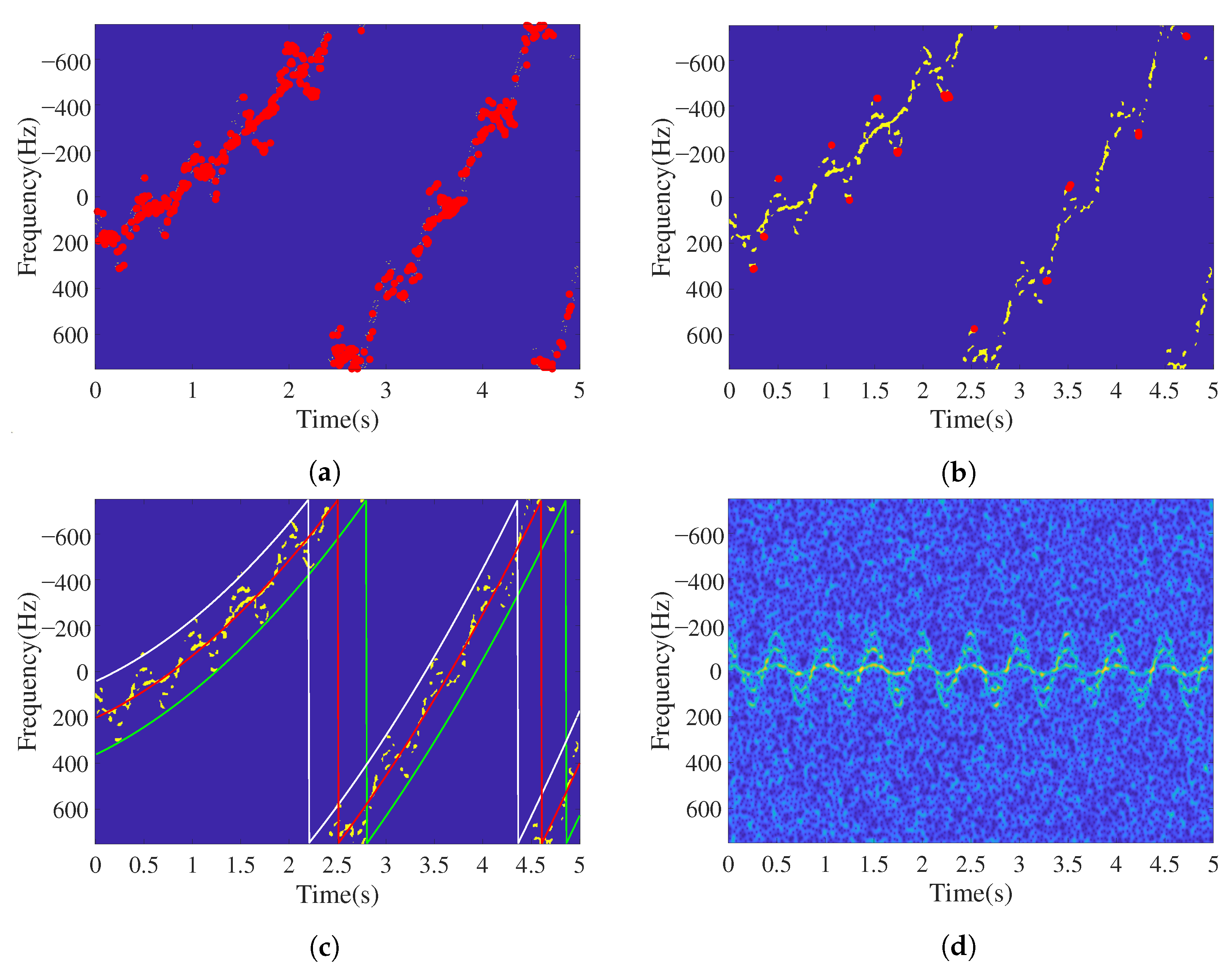
The target’s binarized micro-Doppler signal $f_{md}$ is obtained by time-frequency transformation and binarization of the baseband echo signal. The existence of translation makes it difficult to extract the micro-motion feature of the target. Therefore, it must be effectively and accurately compensated before extracting the micro-motion feature.

Observing the micro-Doppler signal $f_{md}$, it can be found that the intersection of each component and the outer contour of the entire signal provides the best information for translational parameter estimation. However, high time-frequency resolution and a relatively low noise environment are required when using intersection information to estimate the translational parameters, which limits its application. Therefore, this paper uses the external contour of the signal to estimate the translational parameters and achieve the compensation.

To accurately obtain the external contour information of $f_{md}$, the current high-precision edge detection algorithm based on a canny operator [22,23] is used to obtain the external contour of the signal. Then, all of the contour points are obtained through the template matching method, which reflects the target translation. Observing $f_{md}$, as shown in Figure 2, we can see that the local micro-Doppler contour in the white box is parabolic, and multiple protruding points (vertices) can indirectly reflect the overall translation trend of the target. This paper uses this feature to construct a matching template suitable for protruding contour point detection, as shown in Figure 3. The matching template is composed of two parabolas that are symmetrical, up and down, and the sharpness of the micro-Doppler contour of the area to be matched determines the template width $modelW$ and height $modelH$.

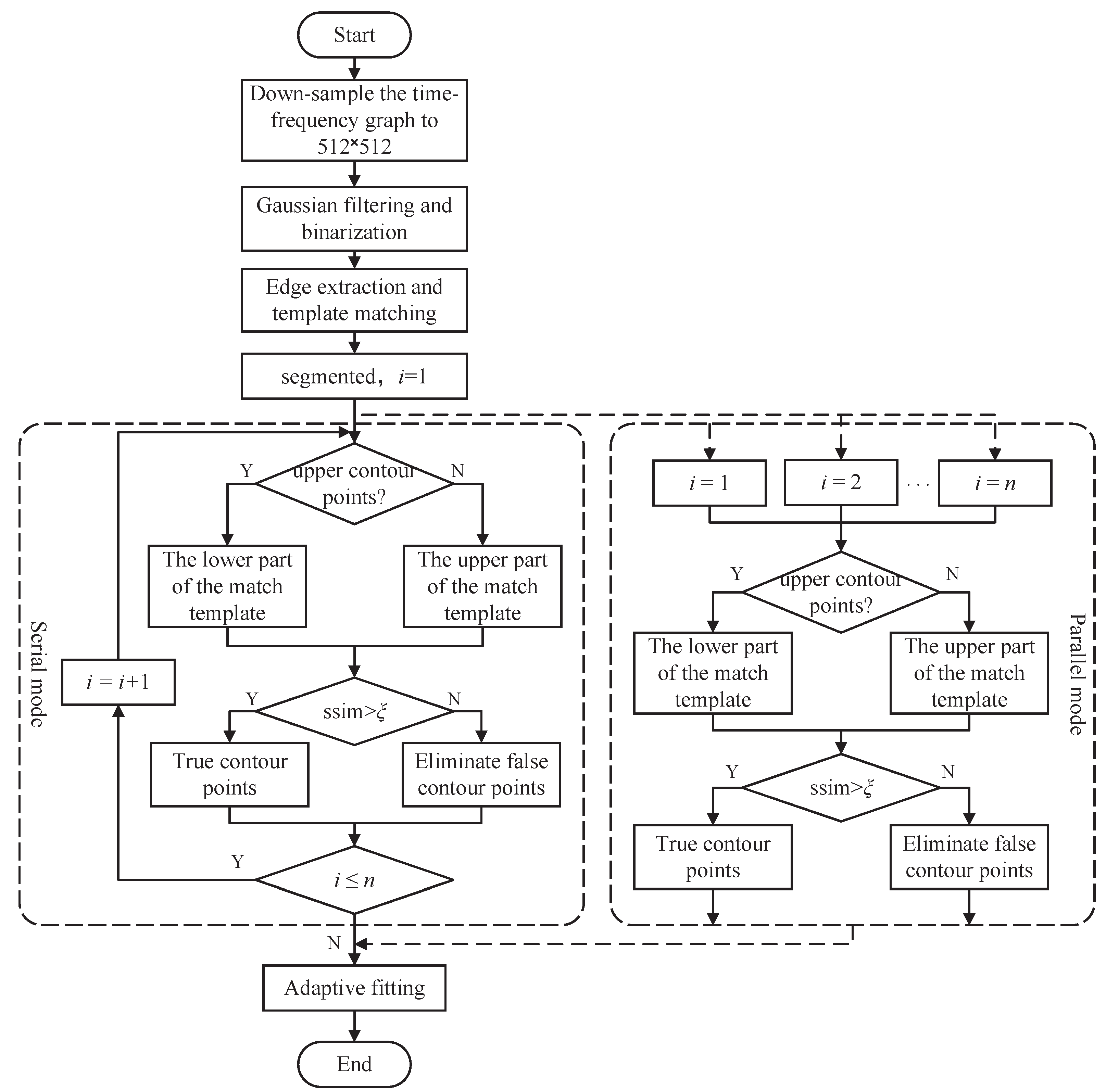
After template matching, the obtained contour points, which we collectively call class contour points, are either true or false. False contour points reduce the estimation accuracy of the translational parameters. This paper adopts the segmentation concept and uses structural similarity to judge and reject false contour points. Finally, the upper and lower trend lines are fitted by an adaptive fitting method. The translational trend line is the average of the two lines above. The following are the specific steps involved:

Step 1: The time-frequency signal $f_{md}$ is obtained by the time-frequency transformation of $s\left(t\right)$.

Step 2: The time–frequency signal $f_{md}$ is downsampled to obtain a 512 × 512 time-frequency diagram $f_{md}^{\prime }$. After Gaussian filtering and binarizing, we obtain $f_{md}^{″}$.

Step 3: Edge detection on $f_{md}^{″}$ is performed based on the canny operator to obtain the envelope $f_{md}^{‴}$ of $f_{md}^{″}$.

Step 4: According to the size of the time-frequency data, a matching template $f_{mod}$, as shown in Figure 2, is constructed. $f_{mod}$ and $f_{md}^{‴}$ are convolved to obtain the matching result.

$$\begin{array}{cc}\hfill f_{mr}(x,y)& =f_{mod}(x,y)*f_{md}^{‴}(x,y)\hfill \\ \hfill & =\sum _{k=0}^{511}\sum _{l=0}^{511}{f}_{mod}(k,l)f_{md}^{‴}(x-k,y-l)\hfill \\ \hfill & =\sum _{k=0}^{modelW-1}\sum _{l=0}^{modelH-1}{f}_{md}^{‴}(k,l)f_{mod}(x-k,y-l)\hfill \\ \hfill & x=0,1,\cdots ,512+modelW-2;y=0,1,\cdots ,512+modelH-2\hfill \end{array}$$

(8)

Step 5: The threshold method is used to preliminarily screen out the class contour points. According to the structural characteristics of the matching template, the threshold is given as $modelW/\phantom{modelW\zeta }\zeta ,\zeta \in R_{+}$. The matching result is further simplified as

$$C_{ont}=\left\{\left.(x,y)\right|f_{mr}(x,y)>modelW/\phantom{modelW\zeta }\zeta \right\}.$$

(9)

Step 6: All class contour points are segmented on the time axis. Then, maximum (and minimum) value is used to determine the preliminary upper and lower contour points.Based on the number of upper and lower protruding points, the segment number n is determined as the addition of the upper and lower contour points minus one. The coordinate sets of the upper and lower contour points are initially obtained as follows.

$$\left\{\begin{array}{c}{C}_{up}=\left\{\left.(x,y)\right|x\in \left[x_i,x_{i+1}\right],\left|y-min{Y}_{ci}\right|<\eta ,(x,y)\in C_{ont}\right\}\hfill \\ C_{down}=\left\{\left.(x,y)\right|x\in \left[x_i,x_{i+1}\right],\left|y-max{Y}_{ci}\right|<\eta ,(x,y)\in C_{ont}\right\}\hfill \end{array}\right.$$

(10)

Among the terms, $\left[x_i,x_{i+1}\right]$ represents the interval of the i-th segment; $Y_{ci}$ is the set of vertical coordinates of points whose abscissas are in the interval $\left[x_i,x_{i+1}\right]$ in the set $C_{ont}$; and $\eta$ is the range threshold which reduces the matching deviation caused by noise.

Step 7: The structural similarity [24] is segmented and used to eliminate false contour points. The structural similarity is calculated between various contour points and the corresponding matching template.

$$\begin{array}{cc}\hfill ssim(f_{mod}^{\prime },f_{mr}^{\prime })& =f(l(f_{mod}^{\prime },f_{mr}^{\prime }),c(f_{mod}^{\prime },f_{mr}^{\prime }),s(f_{mod}^{\prime },f_{mr}^{\prime }))\hfill \\ \hfill & ={\left[l(f_{mod}^{\prime },f_{mr}^{\prime })\right]}^{\upsilon }{\left[c(f_{mod}^{\prime },f_{mr}^{\prime })\right]}^{\vartheta }{\left[s(f_{mod}^{\prime },f_{mr}^{\prime })\right]}^{\gamma }\hfill \end{array}$$

(11)

where:

$$f_{mod}^{\prime }=\left\{\begin{array}{c}(f_{mod}+1)/2,uppercontourpoint\hfill \\ (1-f_{mod})/2,lowercontourpoint\hfill \end{array}\right.$$

(12)

$$\begin{array}{c}\hfill f_{mr}^{\prime }(x,y,x_c,y_c)=f_{md}^{‴}(x,y),|x-x_c|<modelW/\phantom{modelW2,|y-y_c|<modelH/\phantom{modelH2}2}2,|y-y_c|<modelH/\phantom{modelH2}2,(x_c,y_c)\in C_{up}\cup C_{down}\end{array}$$

(13)

$$l(f_{mod}^{\prime },f_{mr}^{\prime })=\frac{2{\mu }_{f_{mod}^{\prime }}{\mu }_{f_{mr}^{\prime }}+C_1}{{\mu }_{f_{mod}^{\prime }}^2+{\mu }_{f_{mr}^{\prime }}^2+C_1}$$

(14)

$$c(f_{mod}^{\prime },f_{mr}^{\prime })=\frac{2{\sigma }_{f_{mod}^{\prime }}{\sigma }_{f_{mr}^{\prime }}+C_2}{{\sigma }_{f_{mod}^{\prime }}^2+{\sigma }_{f_{mr}^{\prime }}^2+C_2}$$

(15)

$$s(f_{mod}^{\prime },f_{mr}^{\prime })=\frac{{\sigma }_{f_{mod}^{\prime }{f}_{mr}^{\prime }}+C_3}{{\sigma }_{f_{mod}^{\prime }}{\sigma }_{f_{mr}^{\prime }}+C_3}$$

(16)

where $C_1,C_2,C_3$ are constants, $\upsilon ,\vartheta ,\gamma >0$ are parameters used to adjust the relative importance of the three components, and $\mu ,\sigma$ are the average gray level and standard deviation of the matching image, respectively.

$$\mu =\frac{1}{H\times W}\sum _{i=1}^H\sum _{j=1}^{M}X(i,j)$$

(17)

$$\left\{\begin{array}{c}{\sigma }_X={\left(\frac{1}{H+W-1}\sum _{i=1}^H\sum _{j=1}^M{(X(i,j)-{\mu }_X)}^2\right)}^{\frac{1}{2}}\hfill \\ {\sigma }_{XY}={\left(\frac{1}{H+W-1}\sum _{i=1}^H\sum _{j=1}^M\left(X(i,j)-{\mu }_X\right)\left(Y(i,j)-{\mu }_Y\right)\right)}^{\frac{1}{2}}\hfill \end{array}\right.$$

(18)

The false contour points are removed and the set of upper and lower true contour points obtained as

$$\left\{\begin{array}{c}{C}_{tup}=\left\{\left.(x_c,y_c)\right|ssim(f_{mod}^{\prime },f_{mr}^{\prime }(x,y,x_c,y_c))>\xi ,(x_c,y_c)\in C_{up}\right\}\hfill \\ C_{tdown}=\left\{\left.(x_c,y_c)\right|ssim(f_{mod}^{\prime },f_{mr}^{\prime }(x,y,x_c,y_c))>\xi ,(x_c,y_c)\in C_{down}\right\}.\hfill \end{array}\right.$$

(19)

where $C_{tup}$ and $C_{tdown}$ are the final coordinate sets of the upper and lower contour points, respectively, and $\xi$ is the structure similarity threshold.

Step 8: Whether there is aliasing in the spectrum is determined. The points in $C_{tup}$ are arranged in ascending order of the abscissa to obtain $C_{tup}^{sort}=\left\{(x_{c1},y_{c1}),(x_{c2},y_{c2}),···,(x_{cK},y_{cK})\right\}$. The ordinate difference $\Delta y_c$ is calculated between adjacent points. It is considered that there is aliasing when $\Delta y_c>\Delta$. Otherwise, there is no aliasing. $\Delta$ is generally half the height of the matching template.

Step 9: According to Step 6 and Step 7, the upper and lower trend lines are fitted. To better adapt to the translational motion under different orders, and to accomplish the adaptive determination of the translational order, the fitting order in Step 7 should satisfy the following conditions

$$k+1=\underset{j}{argmax}(b_j<\epsilon ),j=1,2,3,\dots ,$$

(20)

where k is the translational order, $b_j$ is the coefficient of each order of the fitted polynomial, and $\epsilon$ is the effective lower bound of the coefficient.

The average value of the upper and lower trend lines is taken to estimate the target residual translational velocity $\widehat{v}$ and the first- and second-order acceleration ${\widehat{a}}_1,{\widehat{a}}_2$.

$$\widehat{v}=\frac{\lambda }{2}\left(\frac{f_s}{2}-\frac{b_3{f}_s}{H}\right)$$

(21)

$${\widehat{a}}_1=-\frac{W{b}_2\lambda f_s}{4TH}$$

(22)

$${\widehat{a}}_2=-\frac{W^2{b}_1\lambda f_s}{6T^{2}H}$$

(23)

In Formulas (21)–(23), $f_s$ is the sampling frequency, W is the matching template width, H is the matching template height, and T is the observation time. $b_1,b_2,b_3$ are the second-order, first-order and zero-order term coefficients of the fitted translational trend equation, respectively.

The baseband echo signal after compensation is

$$s_c\left(t\right)=s\left(t\right)·exp\left\{j\frac{4\pi }{\lambda }\left(\widehat{v}t+{\widehat{a}}_1{t}^2+{\widehat{a}}_2{t}^3\right)\right\}.$$

(24)

Taking into account the time complexity of the algorithm, the false contour point elimination in Step 7 can be processed in parallel, which can greatly reduce the running time.

The algorithm flowchart is shown in Figure 4.

4. Simulation and Discussion

In this section, simulation analysis is carried out on the effectiveness and anti-noise quality of the algorithm. In Section 4.1, the effectiveness of the proposed algorithm, based on the short-time Fourier transform (STFT) results in the absence of spectral aliasing, is verified. Then, for different time-frequency analysis methods, the proposed algorithm is simulated and the methods are compared to assess differences in performance. In Section 4.2, the validity of the algorithm for spectral aliasing is determined for noise-free and noisy environments.

4.1. Simulation and Analysis without Spectrum Aliasing

For the simulation, the parameters are taken to be as follows:

The radar carrier frequency is assumed to be 6 GHz. The observation time is 4 s. The radius of the bottom surface of the cone ballistic target is $r=0.6$ m, the distance from the top of the cone to the center of gravity $h_1=2.6$ m, and the distance from the bottom of the cone to the center of gravity $h_2=0.9$ m. The precession angle $\theta ={10}^{\circ }$ and the precession angular velocity ${\omega }_c=4\pi$ rad/s. The angle between the line of sight of the radar and spin axis is $\beta =2\pi /\phantom{2\pi 3}3$ rad. The pitch angle $\alpha =3\pi /\phantom{3\pi 4}4$ rad. The target residual velocity, first-order acceleration, and second-order acceleration after coarse compensation are −21 m/s, 0.5 m/s${}^2$ and 0.3 m/s${}^3$, respectively.

Table 1. Simulation parameter settings.

Parameter	Value
carrier frequency $f_0$	6 GHz
sampling rate $f_s$	2000 Hz
sampling time t	4 s
bottom radius r	0.6 m
distance from top to gravity $h_1$	2.6 m
distance from gravity to bottom $h_2$	0.9 m
angular velocity of the cone ${\omega }_c$	$4\pi$ rad/s
angle between LOS and spin axis $\beta$	$2\pi /\phantom{2\pi 3}3$ rad
pitch angle $\alpha$	$3\pi /\phantom{3\pi 4}4$ rad
residual velocity v	−21.0000 m/s
first-order acceleration $a_1$	0.5000 m/s${}^2$
second-order acceleration $a_2$	0.3000 m/s${}^3$

shows all simulation parameters.

The above simulation parameters are used to obtain the target baseband echo signal, and the time-frequency result shown in Figure 5 is obtained through STFT. The contour points shown in the figure are the target points and indirectly reflect the translational trend of the target.

The time-frequency signal is downsampled to obtain a 512 × 512 grayscale image of the time-frequency signal. Gaussian smoothing is performed on the Gaussian space mask with 1 × 1 pixels and binarized to obtain the binary image of the time-frequency signal.

Edge detection is performed on the binarized time-frequency signal based on the canny operator to obtain the envelope of the time-frequency signal. The 31 × 15 matching template is convolved with the edge detection result map and preliminary screening performed, as shown in Figure 6. As the match result shows, the red dots in the figure represent all the class contour points. In addition to the real contour points in the figure, false contour points occur in the middle of the entire curve, which seriously affect the fitting of the upper and lower trend lines and need to be eliminated.

All contour points are divided into 15 segments on the time axis. All pseudo-contour points are eliminated according to the standard in Step 6 and Step 7 of the second section; the result is shown in Figure 7. From Figure 7, it can be seen that all the false contour points are eliminated and the true contour points are completely retained. This provides an excellent basis for subsequent fitting of the upper and lower trend lines.

According to the standard described in Formula (20), we set $\epsilon ={10}^{-5}$, and obtain the fitting order of the upper and lower trend lines as two. The upper and lower trend lines are fitted and the average of the two taken. The estimated residual velocity, first-order acceleration, and second-order acceleration are $\widehat{v}=-21.0026$ m/s, ${\widehat{a}}_1=0.4973$ m/s${}^2$ and ${\widehat{a}}_2=0.2972$ m/s${}^3$, respectively. The fitting result is shown in Figure 8. The white, green and red lines in the figure are the upward trend line, the downward trend line and the overall translational trend line, respectively. The signal is compensated with the estimated value; the result is shown in Figure 9. The effect of the target translation is completely eliminated.

The above simulation was performed in a noise-free environment. However, it is difficult to achieve a noise-free environment in practice. Therefore, it was necessary to test the algorithm’s effectiveness in a noisy environment. Gaussian white noise with SNR = −4 dB was added to the above simulation echo. The translation parameters were again estimated by the proposed algorithm; Figure 10 shows the results. The estimated translation parameters were $\widehat{v}=-20.8790$ m/s, ${\widehat{a}}_1=0.4803$ m/s${}^2$ and ${\widehat{a}}_2=0.3127$ m/s${}^3$, respectively. Compared with the results in the noise-free environment, the estimation accuracy was reduced.

To accurately test the stability of the algorithm with different SNR, Gaussian white noise of −6 dB∼8 dB was added to the echo.

Table 2. Estimated results of translational parameters of the proposed algorithm under different SNR.

Real Value		$\mathit{v}=-21.0000$ (m/s)	${\mathit{a}}_1=0.5000$ (m/s${}^2$)	${\mathit{a}}_2=0.3000$ (m/s${}^3$)
Estimated value	8 dB	−20.9984	0.5006	0.3019
	6 dB	−21.0269	0.5006	0.2994
	4 dB	−21.0046	0.5072	0.2974
	2 dB	−20.9949	0.5010	0.2935
	0 dB	−21.0113	0.4864	0.2947
	−2 dB	−21.0066	0.4933	0.3116
	−4 dB	−20.8790	0.4803	0.3127
	−6 dB	−21.1823	0.5373	0.2916

shows the translation parameter estimation results obtained by the proposed algorithm with different SNR. From Table 2, it can be inferred that, with decrease in the SNR, the deviation between the estimated value and the actual value of the translation parameter increases. However, the estimation accuracy is still maintained at a high level.

Then, in light of the time-frequency resolution and time complexity, the performance differences between the proposed algorithm, corner detection algorithm and (extended) Hough/Radon transform algorithm, for different time-frequency-analysis methods, were tested. Firstly, 100 Monte Carlo experiments were performed for each of the three algorithms based on STFT [25], as shown in Figure 5. Figure 11 shows the results for estimated relative error under different signal-to-noise ratio conditions.

From Figure 11, it can be seen that, based on the STFT data, the estimation accuracy of the proposed algorithm was higher than that of the (extended) Hough transform method and was equivalent to that of the corner detection method. For the first-order acceleration, the estimation accuracy was generally higher than that of the other two methods. However, the estimation accuracy for the second-order acceleration was lower than that of the other two methods. With respect to algorithm time complexity, the proposed algorithm was superior to the other algorithms. On a computer with a 64-bit Windows 10 operating system, 16 GB RAM and AMD processor in the simulation environment, the running time of the proposed algorithm was approximately 0.2258 s. The running time of the corner detection algorithm was approximately 0.6268 s, and that of the Hough transform algorithm was approximately 6.2053 s.

Secondly, the pseudo-Wigner–Ville distribution (PWVD) [26] was used to obtain the time-frequency distribution, as shown in Figure 12. In contrast to the compromised performance of the time-frequency resolution of STFT, comparing Figure 5 and Figure 12, it was observed that the time-frequency resolution of PWVD was significantly higher than that of STFT. However, the cross-terms between the different components also reduced the internal sharpness of the time-frequency diagram. As a result, theoretically, the estimation accuracy of the three algorithms would be reduced. To verify this conjecture, Figure 13 shows the results of 100 Monte Carlo experiments on each of the three algorithms based on PWVD.

Comparing Figure 11 and Figure 13, it can be seen that the estimation accuracy of the corner detection algorithm decreased, being affected by the cross-term. The estimation accuracy of the proposed algorithm was higher than that of the corner detection algorithm in the range of the test SNR, and slightly lower than that of the Hough transform method. The time complexity was essentially consistent with the above results.

Finally, the time-frequency diagram obtained by the Gabor transform [27], as illustrated in Figure 14, was used to test the accuracy of the proposed algorithm under the same conditions. Figure 15 shows the curve of the relative error of each parameter estimation with different SNR.

Compared with STFT and PWVD, the echo time-frequency distribution obtained by the Gabor transform had a higher time-frequency resolution and higher energy concentration. In theory, all translation compensation methods based on time-frequency analysis can achieve high estimation accuracy. The results shown in Figure 15 support this. The relative error of the estimate was lower than that of the previous two results. When the estimation results based on the Gabor transform were analyzed separately, it was observed that the estimated relative error of the proposed algorithm for residual velocity and first-order acceleration was lower than that of the other algorithms. In other words, the proposed algorithm was able to achieve a higher-precision compensation effect. In addition, the estimation accuracy of second-order acceleration was comparable to that of the other two algorithms. In general, the overall estimation accuracy of the algorithm was better than that of the other algorithms.

In the absence of spectral aliasing, overall, the proposed algorithm had lower requirements with respect to time-frequency resolution than the corner detection algorithm but higher requirements than the Hough transform method. In terms of estimation accuracy, the proposed algorithm was more accurate than the corner detection method and was comparable to the Hough change method. Moreover, the time complexity was lower than in the other two algorithms.

4.2. Simulation and Analysis with Spectrum Aliasing

In practice, spectrum aliasing occurs when the sampling rate does not satisfy the Nyquist sampling theorem. The simulation experiment was repeated to verify the effectiveness of the proposed algorithm in the case of spectrum aliasing. The residual velocity, first-order acceleration and second-order acceleration of the target were assumed to be −5.0 m/s, 2.5 m/s${}^2$ and 0.6 m/s${}^3$, respectively. The sampling frequency was reduced and the observation time increased to 5 s. Meanwhile, other parameters remained unchanged. When noise was absent, the time-frequency diagram for spectral aliasing was obtained as shown in Figure 16.

Figure 17 shows the translation compensation results obtained by the proposed algorithm. The estimated translation parameters were $\widehat{v}=-5.0767$ m/s, ${\widehat{a}}_1=2.5018$ m/s${}^2$ and ${\widehat{a}}_2=0.5994$ m/$s^3$, respectively. Correspondingly, the estimated relative errors of each parameter were 1.53%, 0.07%, and 0.10%, respectively. Compared with the simulation results obtained without spectral aliasing, the proposed algorithm was also effective and met the accuracy requirements in the case of spectral aliasing. The average operation time of the 100 Monte Carlo experiments was approximately 0.3468 s.

The proposed algorithm was used to process the echo signal with SNR = −4 dB for the translation compensation effect with noise and spectrum aliasing; the result is shown in Figure 18. The estimated translation parameters were $\widehat{v}=-5.1036$ m/s, ${\widehat{a}}_1=2.4948$ m/s${}^2$ and ${\widehat{a}}_2=0.6017$ m/s${}^3$, respectively. Combining the translation parameter estimation results and Figure 18, it was found that the parameter estimation accuracy of the proposed algorithm was lower than that of the noise-free case. However, the estimation error was still small. The estimated relative error of each parameter was 2.07%, 0.21% and 0.28%, respectively.

In summary, in the case of spectral aliasing, the estimation accuracy of the proposed algorithm was essentially the same as that in the case of no aliasing. However, the running time of the algorithm was increased compared with that without aliasing at the same time. The other translation compensation algorithms based on time-frequency analysis failed in this case.

5. Conclusions

To address damage to the micro-Doppler structure caused by the high-speed movement of the ballistic target, this paper proposed a translational compensation method based on template matching, which would effectively eliminate the adverse effects of the target’s translational motion. First, binarized time-frequency data were obtained through Gaussian filtering and binarization. A matching template was designed according to the characteristics of the micro-Doppler curve, and the matching template was convolved with the binary time-frequency map to obtain all class contour points. The structural similarity was used to filter out all the true contour points on the basis of obtaining the upper and lower contour points preliminarily by segmenting the maximum and minimum value. Finally, a polynomial fitting method was used to estimate the target translational parameters to achieve full compensation. Simulation results showed that, in the absence of spectral aliasing, as a whole, the proposed algorithm had lower requirements with respect to time-frequency resolution than the corner detection algorithm, but higher requirements than the Hough transform method. In terms of estimation accuracy, the proposed algorithm was more accurate than the corner detection method and was comparable to the Hough change method. Moreover, the time complexity was lower than that of the other two algorithms. In the case of spectral aliasing, the estimation accuracy of the proposed algorithm was essentially the same as that in the case of no aliasing. However, the running time of the algorithm was increased compared with the case without aliasing at the same time. In all other respects, the other translation compensation algorithms based on time-frequency analysis failed directly in this case.

References

1. Chen, V.C. Advances in applications of radar micro-Doppler signatures. In Proceedings of the 2014 IEEE Conference on Antenna Measurements Applications (CAMA), Antibes, France, 16–19 November 2014. [Google Scholar] [CrossRef]
2. Chen, V.C.; Li, F.; Ho, S.S.; Wechsler, H. Micro-Doppler effect in radar: Phenomenon, model, and simulation study. IEEE Trans. Aerosp. Electron. Syst. Trans. Aerosp. Electron. Syst. 2006, 42, 2–21. [Google Scholar] [CrossRef]
3. Chen, V.C. Doppler signatures of radar backscattering from objects with micro-motions. IET Signal Process. 2008, 2, 291–300. [Google Scholar] [CrossRef]
4. Gao, H.; Xie, L.; Wen, S.; Kuang, Y. Research on the influence of acceleration on micro-Doppler and its compensation. J. Astronaut. 2009, 30, 705–711. [Google Scholar] [CrossRef]
5. Wang, Y.; Feng, C.; Zhao, S.; Chen, B. Translational motion compensation of ballistic targets in midcourse based on 2D spectral vector. Transducer Microsyst. Technol. 2017, 36, 66–69. [Google Scholar]
6. Gu, F.; Fu, M.; Liang, B.; Li, K.; Zhang, Q. Translational motion compensation and micro-Doppler feature extraction of space spinning targets. IEEE Geosci. Remote Sens. Lett. 2018, 15, 1550–1554. [Google Scholar] [CrossRef]
7. Li, J.; He, S.; Feng, C.; Wang, Y. Method for compensating translational motion of rotationally symmetric target based on local symmetry cancellation. J. Syst. Eng. Electron. 2017, 28, 36–39. [Google Scholar] [CrossRef]
8. Feng, C.; Yang, Y.; Tong, N. Macro-motion compensation and micro-Doppler zooming by multi-level delayed and conjugated multiplication. In Proceedings of the 2012 Spring Congress on Engineering and Technology, Xi’an, China, 27–30 May 2012. [Google Scholar] [CrossRef]
9. Wei, S.; Wang, J.; Sun, J.; Mao, S. A state space method for estimating the translational radial velocity of ballistic targets. J. Electron. Inf. Technol. 2013, 35, 413–418. [Google Scholar] [CrossRef]
10. Wang, Y.; Feng, C.; Dan, X. Micro-Doppler separation for target with rotating parts based on wavelet decomposition. In Proceedings of the 2016 CIE International Conference on Radar (RADAR), Guangzhou, China, 10–13 October 2016. [Google Scholar] [CrossRef]
11. Xu, D.; Dong, H.; Feng, C.; Geng, Z. Translational motion compensation of ballistic target based on radon transform. In Proceedings of the 2017 3rd IEEE International Conference on Computer and Communications (ICCC), Chengdu, China, 13–16 December 2017. [Google Scholar] [CrossRef]
12. Li, Y.; Li, J.; Liu, F. Ballistic target translation compensation based on corner detection algorithm. In Proceedings of the 2021 IOP Conference Series: Earth and Environmental Science, Xi’an, China, 18–19 December 2020. [Google Scholar] [CrossRef]
13. Han, L.; Tian, B.; Feng, C.; He, S. Translation compensation and resolution of ballistic target with precession. J. Beijing Univ. Aeronaut. Astronaut. 2019, 45, 1459–1466. [Google Scholar] [CrossRef]
14. Chen, J.; Luo, S.; Cen, C.; Li, C.; Qi, J. Translation compensation of space targets via image quality. J. Spacecr. TT C Technol. 2017, 36, 014–018. [Google Scholar]
15. Dong, L.; Zhan, M.; Liu, H.; Yong, L.; Liao, G. A robust translational motion compensation method for ISAR imaging based on keystone transform and fractional Fourier transform under low SNR environment. J. Beijing Univ. Aeronaut. Astronaut. 2017, 53, 2140–2156. [Google Scholar] [CrossRef]
16. Guo, L.; Hu, Y.; Dong, X.; Li, M. Translation compensation and micro-motion parameter estimation of laser micro-Doppler effect. Acta Phys. Sin. Chin. Ed. 2018, 67, 150701. [Google Scholar] [CrossRef]
17. Wang, Y.; Feng, C.; Zhang, Y.; He, S. Translational motion compensation of space micromotion targets using regression network. IEEE Access 2019, 7, 155038–155047. [Google Scholar] [CrossRef]
18. Zhang, W.; Li, K.; Jiang, W. Micro-motion frequency estimation of radar targets with complicated translations. AEUE Int. J. Electron. Commun. 2015, 69, 903–914. [Google Scholar] [CrossRef]
19. Zhang, D.; Feng, C.; Zhang, Y.; Li, J. Translation compensation based on cycle subtracting of micro-Doppler curve. Appl. Mech. Mater. 2015, 742, 281–285. [Google Scholar] [CrossRef]
20. Chen, J.; Xing, M.; Yu, H.; Liang, B.; Peng, J.; Sun, G. Motion compensation/autofocus in airborne synthetic aperture radar: A review. IEEE Geosci. Remote Sens. Mag. 2022, 10, 185–206. [Google Scholar] [CrossRef]
21. Ma, L.; Liu, J.; Wang, T.; Li, Y.; Wang, X. Micro-Doppler characteristics of sliding-type scattering center on rotationally symmetric target. Sci. China Inf. Sci. 2011, 54, 1957–1967. [Google Scholar] [CrossRef]
22. Canny, J. A computational approach to edge detection. IEEE Trans. Pattern Anal. Mach. Intell. 1986, 8, 679–698. [Google Scholar] [CrossRef]
23. Dhillon, D.; Chouhan, R. Enhanced edge detection using SR-guided threshold maneuvering and window mapping: Handling broken edges and noisy structures in canny edges. IEEE Access 2022, 10, 11191–11205. [Google Scholar] [CrossRef]
24. Wang, Z.; Bovik, A.C.; Sheikh, H.R.; Simoncelli, E.P. Image quality assessment: From error visibility to structural similarity. IEEE Trans. Image Process. 2004, 13, 600–612. [Google Scholar] [CrossRef] [Green Version]
25. Griffin, D.W.; Lim, J.S. Signal estimation from modified short-time Fourier transform. IEEE Trans. Acoust. Speech Signal Process. 1984, 32, 236–243. [Google Scholar] [CrossRef]
26. Moss, J.C.; Adamopoulos, P.G.; Hammond, J.K. Time-frequency distributions: A modification applied to the pseudo-Wigner-Ville distribution and the spectrogram. In Proceedings of the IEEE International Symposium on Circuits and Systems, Portland, OR, USA, 8–11 May 1989. [Google Scholar] [CrossRef]
27. Szmajda, M.; Górecki, K.; Mroczka, J. Gabor transform, SPWVD, Gabor-Wigner transform and wavelet transform—tools for power quality monitoring. Metrol. Meas. Syst. 2010, 17, 383–396. [Google Scholar] [CrossRef] [Green Version]
Figure 1. Ballistic target precession model.
Remotesensing 14 03678 g001
Figure 2. Echo time–frequency diagram.
Remotesensing 14 03678 g002
Figure 3. Matching template. (a) Continuous matching template. (b) Discrete matching template.
Remotesensing 14 03678 g003
Figure 4. Flowchart of translational compensation algorithm based on template matching.
Remotesensing 14 03678 g004
Figure 5. Time-frequency diagram of target echo after coarse compensation.
Remotesensing 14 03678 g005
Figure 6. Edge detection and template matching preliminary screening results.
Remotesensing 14 03678 g006
Figure 7. Pseudo-contour point removal result.
Remotesensing 14 03678 g007
Figure 8. Upper and lower trend lines and overall translational trend fitting results.
Remotesensing 14 03678 g008
Figure 9. Translational full compensation result.
Remotesensing 14 03678 g009
Figure 10. Translation compensation results of the proposed algorithm for SNR = −4 dB and without spectral aliasing. (a) Edge detection and template matching preliminary screening results. (b) Pseudo-contour point removal result. (c) Upper and lower trend lines and overall translational trend fitting results. (d) Translational full compensation result.
Remotesensing 14 03678 g010
Figure 11. Variation curve of relative error of translation parameter estimation with different algorithms based on STFT with SNR. (a) Relative error of velocity. (b) Relative error of first-order acceleration. (c) Relative error of second-order acceleration.
Remotesensing 14 03678 g011
Figure 12. Time-frequency distribution of echoes by PWVD.
Remotesensing 14 03678 g012
Figure 13. Variation curve of relative error of translation parameter estimation with different algorithms based on PWVD with SNR. (a) Relative error of velocity. (b) Relative error of first-order acceleration. (c) Relative error of second-order acceleration.
Remotesensing 14 03678 g013
Figure 14. Time-frequency distribution of echoes by Gabor.
Remotesensing 14 03678 g014
Figure 15. Variation curve of relative error of translation parameter estimation with different algorithms based on Gabor with SNR. (a) Relative error of velocity. (b) Relative error of first-order acceleration. (c) Relative error of second-order acceleration.
Remotesensing 14 03678 g015
Figure 16. Time-frequency diagram of target echo with spectrum aliasing.
Remotesensing 14 03678 g016
Figure 17. Translation compensation results of the proposed algorithm in the case of noise-free environment and spectral aliasing. (a) Edge detection and template matching preliminary screening results. (b) Pseudo-contour point removal result. (c) Upper and lower trend lines and overall translational trend fitting results. (d) Translational full compensation result.
Remotesensing 14 03678 g017
Figure 18. Translation compensation results of the proposed algorithm in the case of noise and spectral aliasing. (a) Edge detection and template matching preliminary screening results. (b) Pseudo-contour point removal result. (c) Upper and lower trend lines and overall translational trend fitting results. (d) Translational full compensation result.
Remotesensing 14 03678 g018