Article

Theory of Microwave Remote Sensing of Vegetation Effects, SoOp and Rough Soil Surface Backscattering

1
Radiation Laboratory, Department of Electrical Engineering and Computer Science, University of Michigan, Ann Arbor, MI 48109, USA
2
Division of Geological and Planetary Sciences, California Institute of Technology, Pasadena, CA 91125, USA
*
Author to whom correspondence should be addressed.
Remote Sens. 2022, 14(15), 3640; https://doi.org/10.3390/rs14153640
Submission received: 14 June 2022 / Revised: 18 July 2022 / Accepted: 20 July 2022 / Published: 29 July 2022
(This article belongs to the Special Issue Advances on Radar Scattering of Terrain and Applications)

Abstract

:
In this paper, we provide updates on our recent work on the theory of microwave remote sensing for applications in remote sensing of soil moisture and snow water equivalent (SWE). The three topics are the following. (i) For the effects of forests and vegetation, we developed the hybrid method of NMM3D full-wave simulations over the vegetation field and forest canopies. In the hybrid method, we combined the use of commercial off-the-shelf software and wave multiple scattering theory (W-MST). The results showed much larger transmission than classical radiative transfer theory. (ii) In signals of opportunity at L-band and P-band, which are radar bistatic scattering in the vicinity of the specular direction, we developed the Analytical Kirchhoff solution (AKS) and Numerical Kirchhoff approach (NKA) in the calculations of coherent waves and incoherent waves. We also took into account of the effects of topographical elevations and slopes which have strong influences. (iii) In rough surface radar backscattering, we used the volume integral equation approach for NMM3D full-wave simulations for soil surfaces with kh up to 15. The simulations were calculated for the X-band and Ku-band and the results showed saturation effects. The simulation results can be applied to microwave remote sensing of SWE at these two frequencies.

1. Introduction

Soil moisture and snow water equivalent are two geophysical variables that are monitored globally and continually. Information of soil moisture has applications in weather forecasting, modeling of climate change, agricultural productivity, water resources management, drought prediction, flood area mapping, and the ecosystem. Seasonal snow on land is responsible for processes and feedbacks that affect the global climate system, freshwater availability to billions of people, biogeochemical activity including exchanges of carbon dioxide and trace gases, and ecosystem services.
Presently, the ESA SMOS satellite and NASA SMAP satellite have been using L-band radiometry in measuring soil moisture. The NISAR satellite that will be launched in 2023 will use both L-band and S-band radar backscattering. The ESA’s Sentinel 1 radar at C-band has also been used to map soil moisture. The Copernicus Imaging Microwave Radiometer (CIMR) will be launched by ESA. There are five frequencies in CIMR of which the L-band, C-band, and X-band will be useful for the monitoring of soil moisture. Recently, P-band reflectometry is also proposed for the remote sensing of soil moisture. In microwave remote sensing of soil moisture, a major challenge is the ability of microwaves to penetrate through the vegetation field and forest canopies above the soil. The original proposal of SMAP at L-band was that the sensitivity to soil moisture will be limited by the vegetation field and forest canopies with the upper limit of VWC (Vegetation Water Content) at 5 kg/m2. This upper limit is based on the models of radiative transfer equation (RTE) and the distorted Born approximation (DBA) using the discrete scatterer model. The RTE and DBA approaches have been used since the 1980s and are extensions of the water cloud model [1]. Based on the two models, attenuation through vegetation will increase with frequency, making it even more difficult for remote sensing of soil moisture at the higher frequencies of S-, C-, and X-bands. However, in recent years, we have been successful in performing full-wave simulations of Numerical solution of Maxwell equations in 3D vegetation based on the hybrid method [2,3,4,5]. The results of full-wave simulations showed much larger transmission than that of the results of RTE/DBA.
In P-band and L-band Signals of Opportunity (SoOp), the transmitters on existing satellites are utilized. Satellites with receivers are launched to measure the reflected signals. Global Navigation Satellite System Reflectometry (GNSS-R) is an application of SoOp at the L-band. The operating GNSS-R missions include the Techdemosat-1 (TDS-1) [6] launched by UK in 2014, the Cyclone Global Navigation Satellite System (CYGNSS) [7] launched by NASA in 2016, and Bufeng launched by China in 2019. The GNSS-R data are collected in the form of Delay Doppler Maps (DDMs). Researchers have shown the potential of soil moisture retrieval by the GNSS-R data [8,9,10]. Recently there are also interests in using the phase of the P-band signals of opportunity at 370 MHz. In Reference [11], it was proposed to infer snow water equivalent using the phase of the reflected waves. With new SAR technology [12] implemented for Signals of Opportunity with much higher spatial resolutions, the use of SoOp will gain importance for remote sensing in land applications. The distinction between SoOp and radar backscattering is that in SoOp, the bistatic direction is in the vicinity of the specular direction within a few degrees. The signals are influenced strongly by topography. In theoretical modeling for signals of opportunity, we developed the Analytical Kirchhoff solution (AKS) and Numerical Kirchhoff approach (NKA) in first-principles calculations of coherent waves and incoherent waves [13,14,15,16].
In microwave remote sensing of snow water equivalent (SWE), the X- and Ku-band radar backscattering measurements provide the means to produce SWE information at the temporal and spatial scales necessary to advance water resource management across the northern hemisphere [17]. The ESA Cold Regions Hydrology High-Resolution Observatory (CoReH2O) mission (dual-frequency X- and Ku-band; completed Phase A at ESA in 2013) was a major impetus [18]. The physical basis for estimating SWE from X- and Ku-band radar measurements is volume scattering by millimeter-scale snow grains. Significant progress was made over the past decade in understanding the X-band and Ku-band radar response to variations in SWE, snow microstructure, and snow wet/dry state. Driven by the success of recent air-borne measurements, ground-based measurements, [19,20,21] and improved physical models and validations of retrieval algorithms [22,23,24], a Terrestrial Snow Mass Mission (TSMM) in phase 0 has been supported by the Canadian Space Agency. In addition to volume scattering, another contribution to the X-band and Ku-band radar backscattering signal is the rough surface backscattering from the soil surface below the snow. The backscattering is the sum of the volume scattering contribution and the rough surface scattering contribution. The rough-surface scattering is a “nuisance effect” as it is not correlated with SWE and needs to be subtracted to obtain the volume scattering contribution. With the advent of computers and computation methods, full-wave simulations of numerical solutions of Maxwell equations for rough soil-surface scattering have been carried out for L-bands up to kh = 3 where k is the wavenumber and h is the rms height [25,26,27]. In mountainous regions, the rms height of rough surfaces can be 6 cm so that kh = 25 at the Ku band frequency of 17.2 GHz
Recently, we performed full-wave simulations to apply to rough-surface scattering at X-band and Ku-band, up to kh = 15 using the volume integral equation (VIE) approach. The results showed rough-surface scattering saturation with increase of rms height and frequency.
The focus of this paper was to present the exciting recent results from our group on the theory of microwave remote sensing. In the three topics, (i) the full-wave simulations of NMM3D are recent works that can provide different results from RTE. It is significant because the models of RTE and a similar model of DBA have been used for several decades. (ii) For the signals of opportunity, the SoOp topic is new as SoOp missions were only recently launched. The new microwave theory is that the scattered direction is in the vicinity of the specular direction. The theory shows that, unlike radar backscattering, specular reflection is affected by topography strongly and there are both coherent waves and incoherent waves. (iii) For rough-surface scattering, the new theory is for kh up to 15 while old models are limited to kh = 3. The new theory means that the results can be applied up to the Ku-band.
In Section 2, we study the effects of forests and vegetation in microwave remote sensing of soil moisture. We describe the hybrid method of NMM3D full-wave simulations over the vegetation scene and forests scene. In Section 3, we describe the model of signals of opportunity. We describe the Analytical Kirchhoff solution (AKS) and Numerical Kirchhoff approach (NKA) in first-principles calculations of coherent waves and incoherent waves in the vicinity of the specular scattered direction. In addition to microwave centimeter roughness, we also took into accounts of the effects of topographical elevations and slopes. The results of NKA and AKS were indistinguishable. Comparisons were also made with the results of two geometric optics methods. In Section 4, we describe NMM3D full-wave simulations of rough soil-surface scattering for soil surfaces with kh up to 15. The simulations were applied for the X-band and Ku-band to calculate rough-surface scattering of the soil surface with and without a layer of snow above the soil. We also illustrate the retrieval of rough surface rms height and soil moisture using UAVSAR L-band data. Section 5 is the Conclusion.

2. Vegetation and Forest Effects in Microwave Remote Sensing of Soil Moisture

In microwave remote sensing of soil moisture, a major challenge is the capability of microwaves to penetrate through the vegetation and forest canopies. The accurate modeling of wave propagation at multiple frequencies in the vegetation layer above the soil is also crucial for evaluating the feasibility of the multifrequency approach of remote sensing of soil moisture.
Since the 1980s, the discrete scatterer approach has been implemented using Radiative Transfer Equation (RTE) and the Distorted Born Approximation (DBA). In these two approaches, the vegetation canopy is considered as a layer of randomly distributed scatterers. Specifically, the branches and leaves are treated as single scatterers and are modeled, respectively, by cylinders and disks. The positions of branches and leaves are assumed to be random and are assumed to be statistically homogeneous in space. The scattering and absorption cross sections are calculated by adding the scattering cross sections and absorption cross sections of each branch and each leaf. The orientations of disks and cylinders are characterized by probability distribution over the Euler angles of rotations [28].
In RTE and DBA, the vegetation or forest canopy is approximated as a layered medium with an effective attenuation rate calculated based on the independent scattering approximation. The effective attenuation rate is basically an assumption of homogenization treating the vegetation canopy as effectively homogeneous. In this model of backscattering, there are three contributions which are rough-surface scattering, volume scattering, and double bounce [29,30]. The models of first-order RTE and DBA are essentially the same as they have the same formulas of attenuation, optical thickness tau, and bistatic volume scattering. The only difference between RTE and DBA is a factor of 2 in the double bounce term, which is due to backscattering enhancement [22,31,32,33]. The RTE and DBA have several inherent approximations when applied to vegetation and forests.
(1) The positions of the scatterers are assumed to be uniformly random. However, such a description is not consistent with the clustering of scatterers in a tree or plant. For example, in pine trees, there are hundreds of needle leaves attached to a branch. In addition, the assumption of uniformly random positions does not account for the gaps among plants and trees. Unlike ray optics, the abilities of microwave to pass through the gaps depend on the sizes of the gaps relative to the microwave wavelength.
(2) The scatterers such as leaves and branches are assumed to be independent so that the scattered intensities are added incoherently. The frequency dependence of scattering is that of the individual cylinder and/or individual disk, which leads to a strong increase of scattering and absorption by vegetation. The collective scattering and absorption effects due to clustering are ignored.
(3) Far-field assumptions are made throughout the RTE and DBA models. This means far field between the scatterers and between the scatterers and the underlying soils. Since the far field distance is size squared divided by wavelength, the far field assumptions are not obeyed in vegetation/forests.
Recently, we were successful in performing full-wave solutions of Numerical Maxwell Model of 3D Simulations. The method is a hybrid method combining Computational Electromagnetics (CEM) of a single object with Wave Multiple Scattering Theory (W-MST). We added a word “Wave” in front of MST to distinguish from the multiple scattering theory of the Radiative Transfer Equations. The MST in RTE is intensity addition rather than wave interactions with amplitudes and phases. In the following subsections, we first describe the T matrix of a single scatterer that can be calculated from CEM. This is followed by the W-MST based on Foldy-Lax equations.
In addition to remote sensing, the MST model has been extensively used in solid state physics, photonics, and acoustics.

2.1. T Matrix of a Plant or a Tree

The W-MST formulation is a Foldy-Lax Multiple Scattering equation using the T matrices of single scatterers. In the hybrid method, we treat a single plant such as a corn plant, a wheat plant, or a soya bean plant, or a single tree as a single scatterer. This is different from the RTE and DBA in that a single branch or a single leaf is treated as a single scatterer. The single scatterer T matrix is the scattering T matrix of an isolated scatterer in the absence of all other scatterers.
Consider cylindrical coordinates ( ρ , ϕ , z ) . The Vector Cylindrical Waves (VCW) that are outgoing are
M ¯ n ( k z , r ¯ ) = [ ρ ^ i n ρ H n ( 1 ) ( k ρ ρ ) ϕ ^ k ρ H n ( 1 ) ( k ρ ρ ) ] e x p ( i k z z + i n ϕ )
N ¯ n ( k z , r ¯ ) = [ ρ ^ i k ρ k z k H n ( 1 ) ( k ρ ρ ) ϕ ^ n k z k ρ H n ( 1 ) ( k ρ ρ ) + z ^ k ρ 2 k H n ( 1 ) ( k ρ ρ ) ] e x p ( i k z z + i n ϕ )
where k is the wavenumber, k ρ = k 2 k z 2 , < k z < , n = 0 , ± 1 , ± 2 , , and H n ( 1 ) ( k ρ ρ ) are Hankel functions of the first kind and of order n . There are two indices, n and k z , for the wave functions. The regular wave functions are the expressions above which Hankel functions are replaced by Bessel functions J n ( k ρ ρ ) .
R g M ¯ n ( k z , r ¯ ) = [ ρ ^ i n ρ J n ( k ρ ρ ) ϕ ^ k ρ J n ( k ρ ρ ) ] e x p ( i k z z + i n ϕ )
R g N ¯ n ( k z , r ¯ ) = [ ρ ^ i k ρ k z k J n ( k ρ ρ ) ϕ ^ n k z k ρ J n ( k ρ ρ ) + z ^ k ρ 2 k J n ( k ρ ρ ) ] e x p ( i k z z + i n ϕ )
In Figure 1, we show a corn plant with height 1.25 m, and the extent of the leaves is to 0.4 m. For the calculation of T matrices from commercial software (such as FEKO or HFSS), we enclose the plant in a cylindrical volume of radius R C = 0.45 m and height 1.3 m as shown in Figure 1. The T matrices results are for the use in Foldy–Lax multiple scattering equations with other corn plants. Other corn plants are enclosed by similar cylinders, and they lie outside the enclosing cylinders of each other.
The T matrices in vector cylindrical waves are for the region ρ > R C to treat wave interactions among plants. The fields above the plant and below the plant for ρ R C do not enter Foldy–Lax multiple scattering equations. After Foldy–Lax equations are solved, the fields in these “inner” regions, ρ R C , can be calculated by Huygen’s principles. In Figure 1, the β is the orientation angle and α is the azimuthal angle for the leaf. They are labeled to characterize the orientations of the stalks and the leaves. These are used traditionally in RTE as each stalk is treated as a single scatterer and each leaf is treated as a single scatterer. Both β and α of leaves and stalks obey orientation distributions. Generally, α is assumed to have uniform distribution between 0 and 2 π . In the hybrid method, we perform orientations differently as we treat a plant as a single scatterer. Each plant is vertical. Thus, the plant itself does not have any β . The plant does have the azimuthal angle which is also assumed to be uniform between 0 and 2 π . We construct a corn field of many plants such that the orientations of leaves and stalks are described by the same distributions as done traditionally. We have several plants such that the distributions of β angles of the stalks and leaves agree with traditional characterizations. The T matrices of these several plants are calculated with commercial software. The α angles are next introduced. The T matrices with α ’s are just rotations of the T matrices without the need of calculations of new T matrices.
The plant or tree is within a “virtual” cylinder of radius R C (Figure 1) based on Wave Multiple Scattering Theory (W-MST), the electric field outside the enclosing cylinder, that is, ρ R C is the sum of E ¯ e x , the “final” exciting field, and E ¯ s , the “final” scattered field. Both E ¯ e x and E ¯ s refer to that of the “single scatterer“, which is inside the enclosing cylinder.
The final exciting field and final scattered field are respectively given by
E ¯ e x ( r ¯ ) = n d k z [ a n E M ( k z ) R g M ¯ n ( k z , r ¯ ) + a n E N ( k z ) R g N ¯ n ( k z , r ¯ ) ]
E ¯ s ( r ¯ ) = n d k z [ a n S M ( k z ) M ¯ n ( k z , r ¯ ) + a n S N ( k z ) N ¯ n ( k z , r ¯ ) ]
In W-MST, the T matrix is that of a single scatterer, which is the scattering of the scatterer in the absence of all other scatterers. The scattered field coefficients are expressed in terms of the T matrices.
a n S M ( k z ) = n d k z [ T n n ( M , M ) ( k z , k z ) a n E M ( k z ) + T n n ( M , N ) ( k z , k z ) a n E N ( k z ) ]
a n S N ( k z ) = n d k z [ T n n ( N , M ) ( k z , k z ) a n E M ( k z ) + T n n ( N , N ) ( k z , k z ) a n E N ( k z ) ]
where the T matrix coefficients are T n n ( M , M ) ( k z , k z ) , T n n ( M , N ) ( k z , k z ) , T n n ( N , M ) ( k z , k z ) , and T n n ( N , N ) ( k z , k z ) . The T matrix coefficients have dimensions of length for this case of cylindrical waves.
The self-consistent equations of W-MST allow E ¯ e x and E ¯ s to be calculated in a self-consistent manner using the single scatterer T matrix. Since < k z < , and k ρ = k 2 k z 2 , the waves are propagating for | k z | k and evanescent in the ρ ^ direction for | k z | > k . Evanescent waves decay exponentially. At 1 / 4 wavelengths, the evanescent waves become small. At the SMAP frequency of 1.41   GHz , this 1 / 4 wavelength corresponds to 5.3   cm . This means if the neighboring circumscribing cylinder is separated by more than 5 cm, the evanescent waves are negligible. We shall truncate with | k z | k . The angular direction θ can be used with
k z = k cos θ ; k k d k z = k 0 π d θ sin θ
In (9) there is a factor, sin θ , that corresponds to the decrease of the solid angle when θ 0 , decreasing the contributions of θ 0 .
The cylindrical wave expansions are analytic wave functions. The use of Bessel functions and Hankel functions in the wave functions M ¯ n and N ¯ n mean that they are applicable to all distance ranges of ρ from near field to intermediate distance and to far field. On the other hand, the coefficients of field expansions, which include exciting field coefficients, the scattered field coefficients, and the T matrix coefficients are independent of distance. This means we can obtain these coefficients at any distance including the far field, the intermediate field, and the near field. Once these coefficients are obtained, they can be substituted in the analytic field expansions and the field expansions are valid for all distance ranges. We use far field to extract the T matrix coefficients because commercial software provides far-field scattering amplitudes.
In the far field, we related the T matrix of vector spherical waves to that of far field scattering amplitudes [28]. Below, we relate the T matrix of vector cylindrical waves (VCW) to the far field scattering amplitudes. In the far field of ρ
M ¯ n ( k z , r ¯ ) ϕ ^ k ρ ( i 2 π k ρ ρ e x p ( i ( k ρ ρ n π 2 π 4 ) ) ) e x p ( i k z z ) e x p ( i n ϕ )
N ¯ n ( k z , r ¯ ) [ ρ ^ k z + z ^ k ρ ] k ρ k 2 π k ρ ρ e x p ( i ( k ρ ρ n π 2 π 4 ) ) e x p ( i k z z ) e x p ( i n ϕ )
Substitute into Equation (6) and apply the method of stationary phase. The spherical coordinates are ( r , θ , ϕ ) . The stationary phase points are at k z = k cos θ , k ρ = k sin θ . Since θ ^ = cos θ ρ ^ sin θ z ^ , then
E ¯ s ( r ¯ ) ϕ ^ k sin θ 2 e x p ( i k r ) r n e x p ( i n π 2 ) e x p ( i n ϕ ) a n S M ( k cos θ ) θ ^ k sin θ 2 e x p ( i k r ) i r n e x p ( i n π 2 ) e x p ( i n ϕ ) a n S N ( k cos θ )
Let the exciting field be a plane wave in the direction k ^ i = sin θ i cos ϕ i x ^ + sin θ i sin ϕ i y ^ + cos θ i z ^ with polarizations vectors v ^ i = θ ^ i of vertical polarization and h ^ i = ϕ ^ i of horizontal polarization. Let the amplitudes be E v i and E h i . Then, from Tsang et al., volume 1 [28]
E ¯ e x ( r ¯ ) = ( v ^ i E v i + h ^ i E h i ) e x p ( i k ¯ i r ¯ ) = n i n e x p ( i n ϕ i ) k i ρ [ i E h i R g M ¯ n ( k i ρ , k i z , r ¯ ) E v i R g N ¯ n ( k i ρ , k i z , r ¯ ) ]
The exciting field coefficients are
a n E M ( k z ) = i n + 1 e x p ( i n ϕ i ) k i ρ E h i δ ( k z k i z )
a n E N ( k z ) = i n e x p ( i n ϕ i ) k i ρ E v i δ ( k z k i z )
where δ ( k z k i z ) is the delta function indicating that k z = k i z . Substitute (14) and (15) into Equations (7) and (8), and we obtain the scattered field coefficients as
a n S M ( k cos θ ) = n T n n ( M , M ) ( k cos θ , k cos θ i ) ( i n + 1 e x p ( i n ϕ i ) k i ρ E h i ) + n T n n ( M , N ) ( k cos θ , k cos θ i ) ( i n e x p ( i n ϕ i ) k i ρ E v i )
a n S N ( k cos θ ) = n T n n ( N , M ) ( k cos θ , k cos θ i ) ( i n + 1 e x p ( i n ϕ i ) k i ρ E h i ) + n T n n ( N , N ) ( k cos θ , k cos θ i ) ( i n e x p ( i n ϕ i ) k i ρ E v i )
The far field scattered field is
E ¯ s ( r ¯ ) = i ϕ ^ k sin θ 2 i e x p ( i k r ) r n e x p ( i n π 2 ) e x p ( i n ϕ ) [ n T n n ( M , M ) ( k cos θ , k cos θ i ) ( i n + 1 e x p ( i n ϕ i ) k i ρ E h i ) + n T n n ( M , N ) ( k cos θ , k cos θ i ) ( i n e x p ( i n ϕ i ) k i ρ E v i ) ] θ ^ k sin θ 2 i e x p ( i k r ) r n e x p ( i n π 2 ) e x p ( i n ϕ ) [ n T n n ( N , M ) ( k cos θ , k cos θ i ) ( i n + 1 e x p ( i n ϕ i ) k i ρ E h i ) + n T n n ( N , N ) ( k cos θ , k cos θ i ) ( i n e x p ( i n ϕ i ) k i ρ E v i ) ]
The far field scattered field is written as
E ¯ s ( r ¯ ) = e x p ( i k r ) r ( v ^ s E v s + h ^ s E h s )
where v ^ s = θ ^ s , h ^ s = ϕ ^ s . The scattered field components E v s and E h s have dimensions of length and are in terms of scattering amplitudes, f v v ( θ , ϕ ; θ i , ϕ i ) , f v h ( θ , ϕ ; θ i , ϕ i ) , f h v ( θ , ϕ ; θ i , ϕ i ) , and f h h ( θ , ϕ ; θ i , ϕ i ) .
E v s = f v v ( θ , ϕ ; θ i , ϕ i ) E v i + f v h ( θ , ϕ ; θ i , ϕ i ) E h i
E h s = f h v ( θ , ϕ ; θ i , ϕ i ) E v i + f h h ( θ , ϕ ; θ i , ϕ i ) E h i
Equations (18)–(21), we obtain
f v v ( θ , ϕ ; θ i , ϕ i ) = k sin θ 2 i n e x p ( i n π 2 ) e x p ( i n ϕ ) [ n T n n ( N , N ) ( k cos θ , k cos θ i ) ( i n e x p ( i n ϕ i ) k i ρ ) ]
f v h ( θ , ϕ ; θ i , ϕ i ) = k sin θ 2 i n e x p ( i n π 2 ) e x p ( i n ϕ ) [ n T n n ( N , M ) ( k cos θ , k cos θ i ) ( i n + 1 e x p ( i n ϕ i ) k i ρ ) ]
f h v ( θ , ϕ ; θ i , ϕ i ) = i k sin θ 2 i n e x p ( i n π 2 ) e x p ( i n ϕ ) [ n T n n ( M , N ) ( k cos θ , k cos θ i ) ( i n e x p ( i n ϕ i ) k i ρ ) ]
f h h ( θ , ϕ ; θ i , ϕ i ) = i k sin θ 2 i n e x p ( i n π 2 ) e x p ( i n ϕ ) [ n T n n ( M , M ) ( k cos θ , k cos θ i ) ( i n + 1 e x p ( i n ϕ i ) k i ρ ) ]
The above expressions indicate that the T matrix coefficients, T n n are Fourier coefficients of the double Fourier series of the far-field scattering amplitudes. Using Fourier coefficients integration, we have
T n n ( N , N ) ( k cos θ , k cos θ i ) = i sin θ i 8 π 2 sin θ i n n 0 2 π d ϕ 0 2 π d ϕ i e x p ( i n ϕ + i n ϕ i ) f v v ( θ , ϕ ; θ i , ϕ i )
T n n ( N , M ) ( k cos θ , k cos θ i ) = sin θ i 8 π 2 sin θ i n n 0 2 π d ϕ 0 2 π d ϕ i e x p ( i n ϕ + i n ϕ i ) f v h ( θ , ϕ ; θ i , ϕ i )
T n n ( M , N ) ( k cos θ , k cos θ i ) = sin θ i 8 π 2 sin θ i n n 0 2 π d ϕ 0 2 π d ϕ i e x p ( i n ϕ + i n ϕ i ) f h v ( θ , ϕ ; θ i , ϕ i )
T n n ( M , M ) ( k cos θ , k cos θ i ) = i sin θ i 8 π 2 sin θ i n n 0 2 π d ϕ 0 2 π d ϕ i e x p ( i n ϕ + i n ϕ i ) f h h ( θ , ϕ ; θ i , ϕ i )
The far-field scattering amplitudes for incident plane waves are computed in commercial software such as FEKO and HFSS.

2.2. Wave Multiple Scattering Theory (W-MST)

Let there be N scatterers. All the scatterers are within enclosing cylinders. The T matrices are used to describe the scattered fields outside the circumscribing cylinders at all distance ranges. Consider an incident wave with incident field E ¯ i n c ( r ¯ ) . For W-MST, the final exciting field on one scatterer, ′ q ′, is the sum of the incident field and the scattered fields from all other scatterers except itself. The Foldy–Lax wave multiple scattering equations are
E ¯ q e x ( r ) = E ¯ i n c ( r ¯ ) + p = 1 , p q N E ¯ q p s ( r ¯ )
where q = 1 , 2 , , N . In (30) E ¯ q e x ( r ) is the “final” exciting field of scatterer q , and E ¯ q p s ( r ¯ ) is the “final” scattered field from scatterer p to scatterer q . In (30), the summation of p is over all scatterers, p = 1 , 2 , , N , with p q . Using cylindrical coordinate system, r ¯ = ρ ¯ + z z ^ , the center location of the q t h scatterer is r ¯ q = ρ ¯ q + z q z ^ = x q x ^ + y q y ^ + z q z ^ . Since the scatterer is inside a circumscribing cylinder, the ρ ¯ q coordinate coincides with the horizontal center of the cylinder. Since each scatterer is enclosed by a cylindrical surface, the final excitation fields can be expanded using the incoming VCW. For scatterer q centered at r ¯ q , E ¯ q e x ( r ) is expanded as
E ¯ q e x ( r ¯ ) = m d k z R g M ¯ m k z , r r ¯ q a m , q E M k z + R g N ¯ k z , r r ¯ q a m , q E N k z
In (31), r r ¯ q = r ¯ r ¯ q , R g M ¯ m ( k z , r r ¯ q ) and R g N ¯ ( k z , r r ¯ q ) are VCW-centered at r ¯ q . The incident plane wave is in direction k ¯ i = k i ρ cos ϕ i x ^ + k i ρ sin ϕ i y ^ + k i z z ^ with k i z = k cos θ i and k i ρ = k sin θ i . The electric field of the incident plane wave is
E ¯ i n c ( r ¯ ) = ( v ^ E v i + h ^ E h i ) e x p ( i k ¯ i · r ¯ )
To balance the Foldy–Lax Equation (30), all terms need to have VCW with the center at the q th scatterer, r ¯ q . To achieve that, we make use of wave transformation. For the incident wave, we set e x p ( i k ¯ i r ¯ ) =   e x p ( i k ¯ i r ¯ q ) e x p ( i k ¯ i ( r ¯ r ¯ q ) ) . A phase shift results when we use the VCW expansion in Equation (13) with center at r ¯ q ,
E ¯ q i n c ( r ¯ ) = d k z e x p i k ¯ i · r ¯ q m i m e x p i m ϕ i k i ρ × i E h i R g M ¯ m k ρ , k z , r r ¯ q E v i R g N ¯ m k ρ , k z , r r ¯ q δ k z k i z
The Dirac delta function δ ( k z k i z ) indicates that the incident wave is with k z = k i z in the integration d k z . Since the scattered field from p to q originates from scatterer p , the outgoing VCW from scatterer p are initially expressed with origin at r ¯ p . The expansion is
E ¯ q p s ( r ¯ ) = n d k z [ M ¯ n ( k z , r r ¯ p ) a n , p S M ( k z ) + N ¯ n ( k z , r r ¯ p ) a n , p S N ( k z ) ]
To translate E ¯ q p s ( r ¯ ) to origin, r ¯ q of q scatterer, we use the translational addition theorem. Let r ¯ p = ρ ¯ p + z p z ^ = x p x ^ + y p y ^ + z p z ^ , ρ p ρ q ¯ = ρ ¯ p ρ ¯ q . The quantity ϕ ρ p ρ q ¯ = t a n 1 y p y q x p x q is the angle that ρ ¯ p ρ ¯ q makes with the x axis. The translational addition theorems are (Tsang et al. volume 2)
M ¯ n ( k z , r r ¯ p ) = m R g M ¯ m ( k z , r r ¯ q ) H m n ( 1 ) ( k ρ | ρ p ρ q ¯ | ) e x p ( i ( m n ) ϕ ρ p ρ q ¯ ) e x p ( i k z ( z p z q ) )
N ¯ n ( k z , r r ¯ p ) = m R g N m ( k z , r r ¯ q ) H m n ( 1 ) ( k ρ | ρ p ρ q ¯ | ) e x p ( i ( m n ) ϕ ρ p ρ q ¯ ) e x p ( i k z ( z p z q ) )
Then we have
E ¯ q p s ( r ¯ ) = n d k z m R g M ¯ m ( k z , r r ¯ q ) H m n ( 1 ) ( k ρ | ρ p ρ q ¯ | ) e x p ( i ( m n ) ϕ ρ p ρ q ¯ ) e x p ( i k z ( z p z q ) ) a n , p S M ( k z ) + n d k z m R g N ¯ m ( k z , r r ¯ q ) H m n ( 1 ) ( k ρ | ρ p ρ q ¯ | ) e x p ( i ( m n ) ϕ ρ p ρ q ¯ ) e x p ( i k z ( z p z q ) ) a n , p S N ( k z )
Since all terms now have the dependence Rg M ¯ m ( k z , r r ¯ q ) or Rg N ¯ m ( k z , r r ¯ q ) , we balance the coefficients of each term. Balancing the terms with Rg M ¯ m ( k z , r r ¯ q ) , we have
a m , q E M k z = e x p i k ¯ i · r ¯ q i m e x p i m ϕ i k i ρ i E h i δ k z k i z + p q n H m n ( 1 ) k ρ ρ p ρ q ¯ × e x p i ( m n ) ϕ ρ p p q ¯ e x p i k z z p z q a n , p S M k z
Balancing Rg N ¯ m ( k z , r r ¯ q ) , we have
a m , q E N k z = e x p i k ¯ i · r ¯ q i m e x p i m ϕ i k i ρ E v i δ k z k i z + p q n H m n ( 1 ) k ρ ρ p ρ q ¯ × e x p i ( m n ) ϕ ρ p ρ q ¯ e x p i k z z p z q a n , p S N k z
The multiple scattering equations in (38) and (39) relate exciting field coefficients a m , q E M ( k z ) , a m , q E N ( k z ) and scattering field coefficients a n , p S M ( k z ) , a n , p S N ( k z ) among the scatterers. To obtain Foldy–Lax equations with the exciting field coefficients a m , q E M ( k z ) , a m , q E N ( k z ) as unknowns, we use the T matrix relations
a n , p S M k z = n d k z T n n , p ( M , M ) k z , k z a n , p E M k z + T n n , p ( M , N ) k z , k z a n , p E N k z
a n , p S N k z = n d k z T n n , p ( N , M ) k z , k z a n , p E M k z + T n n , p ( N , N ) k z , k z a n , p E N k z
Then, the Foldy–Lax MST equations with exciting field coefficients as field unknowns are
a m , q E M k z = e x p i k ¯ i · r ¯ q i m e x p i m ϕ i k i ρ i E h i δ k z k i z + p q n H m n ( 1 ) k ρ ρ p ρ q ¯ e x p i ( m n ) ϕ ρ p ρ q ¯ e x p i k z z p z q × n d k z T n n , p ( M , M ) k z , k z a n , p E M k z + T n n , p ( M , N ) k z , k z a n , p E N k z
a m , q E N k z = e x p i k ¯ i · r ¯ q i m e x p i m ϕ i k i ρ E v i δ k z k i z + p q n H m n ( 1 ) k ρ ρ p ρ q ¯ e x p i ( m n ) ϕ ρ p ρ q ¯ e x p i k z z p z q × n d k z T n n , p ( N , M ) k z , k z a n , p E M k z + T n n , p ( N , N ) k z , k z a n , p E N k z
In solving the Foldy–Lax equations numerically, it is sometimes convenient to use scattered field coefficients as field unknowns. To obtain scattered field coefficients, MST, multiply (38) by m d k z T m m , q ( M , M ) ( k z , k z ) and multiply (39) by m d k z T m m , q ( M , N ) ( k z , k z ) . Adding the two equations gives
a m , q S M k z = m e x p i k ¯ i · r ¯ q i m e x p i m ϕ i k i ρ T m m , q ( M , M ) k z , k i z i E h i T m m , q ( M , N ) k z , k i z E v i + m d k z p q n H m n ( 1 ) k ρ ρ p ρ q ¯ e x p i ( m n ) ϕ ρ p ρ q ¯ e x p i k z z p z q T m m , q ( M , M ) k z , k z a n , p S M k z + T m m , q ( M , N ) k z , k z a n , p S M k z
Next, multiply (38) by m d k z T m m , q ( N , M ) ( k z , k z ) and multiply (39) by m d k z T m m , q ( N , N ) ( k z , k z ) . Add the two equations gives
a m , q S N k z = m e x p i k ¯ i · r ¯ q i m e x p i m ϕ i k i ρ T m m , q ( N , M ) k z , k i z i E h i T m m , q ( N , N ) k z , k i z E v i + m d k z p q n H m n ( 1 ) k ρ ρ p ρ q ¯ e x p i ( m n ) ϕ ρ p ρ q ¯ e x p i k z z p z q T m m , q ( N , M ) k z , k z a n , p S M k z + T m m , q ( N , N ) k z , k z a n , p S M k z
Equations (44) and (45) are the Foldy–Lax W-MST equations with scattered field coefficients as field unknowns. They are also called the self-consistent MST equations. We can also have exciting field Foldy–Lax MST equations by separating out the incident field Dirac delta functions in (42) and (43). Let
a m , q E M k z = e x p i k ¯ i · r ¯ q i m e x p i m ϕ i k i ρ i E h i δ k z k i z + a m , q E O M k z
a m , q E N k z = e x p i k ¯ i · r ¯ q i m e x p i m ϕ i k i ρ E v i δ k z k i z + a m , q E O N k z
where “O” in the superscript a m , q E O M ( k z ) and a m , q E O N ( k z ) stands for from “other” scatterers. Then the integral equations for a m , q E O M ( k z ) and a m , q E O N ( k z ) are
a m , q E O M k z = p q n H m n ( 1 ) k ρ ρ p ρ q ¯ e x p i ( m n ) ϕ ρ p ρ q ¯ e x p i k z z p z q n T n n , p ( M , M ) k z , k i z e x p i k ¯ i · r ¯ p i n e x p i n ϕ i k i ρ i E h i + p q n H m n ( 1 ) k ρ ρ p ρ q ¯ e x p i ( m n ) ϕ ρ p ρ q ¯ e x p i k z z p z q n d k z T n n , p ( M , M ) k z , k z a n , p E O M k z + p q n H m n ( 1 ) k ρ ρ p ρ q ¯ e x p i ( m n ) ϕ ρ p ρ q ¯ e x p i k z z p z q n T n n , p ( M , N ) k z , k i z e x p i k ¯ i · r ¯ p i n e x p i n ϕ i k i ρ E v i + p q n H m n ( 1 ) k ρ ρ p ρ q ¯ e x p i ( m n ) ϕ ρ p ρ q ¯ e x p i k z z p z q n d k z T n n , p ( M , N ) k z , k z a n , p E O N k z
a m , q E O N k z = p q n H m n ( 1 ) k ρ ρ p ρ q ¯ e x p i ( m n ) ϕ ρ p ρ q ¯ e x p i k z z p z q n T n n , p ( N , M ) k z , k i z e x p i k ¯ i · r ¯ p i n e x p i n ϕ i k i ρ i E h i + p q n H m n ( 1 ) k ρ ρ p ρ q ¯ e x p i ( m n ) ϕ ρ p ρ q ¯ e x p i k z z p z q n d k z T n n , p ( N , M ) k z , k z a n , p E O M k z + p q n H m n ( 1 ) k ρ ρ p ρ q ¯ e x p i ( m n ) ϕ ρ p ρ q ¯ e x p i k z z p z q n T n n , p ( N , N ) k z , k i z e x p i k ¯ i · p ¯ p i n e x p i n ϕ i k i ρ E v i + p q n H m n ( 1 ) k ρ ρ ¯ p ρ q e x p i ( m n ) ϕ ρ p ρ q ¯ e x p i k z z p z q n d k z T n n , p ( N , N ) k z , k z a n , p E O N k z
It should be noted that the Foldy–Lax equations are entirely in terms of the wave interactions outside the circumscribing cylinders. Thus, the wave interactions are completely described by the T matrices of the scatterers.

2.3. Final Fields

After solving the Foldy–Lax MST equations, the final fields both outside and inside the circumscribing cylinders can be calculated by the following procedures.

2.3.1. Outside the Enclosing Cylinders

We obtained the scattered field coefficients from solutions of the Foldy–Lax W-MST equations. Outside the enclosing cylinder, the electric field is equal to the sum of the incident fields and the scattered fields from all the scatterers
E ¯ ( r ¯ ) = E ¯ i n c ( r ¯ ) + q = 1 N E ¯ q s ( r ¯ )
The final scattered fields are calculated by
E ¯ q s ( r ¯ ) = n d k z [ M ¯ n ( k z , r r ¯ q ) a n , q S M ( k z ) + N ¯ n ( k z , r r ¯ q ) a n , q S N ( k z ) ]

2.3.2. Inside the Enclosing Cylinders

By solving the Foldy–Lax MST equations, we obtained the final exciting field coefficients a n , q E M ( k z ) , a n , q E N ( k z ) , q = 1 , 2 , , N .
Since commercial software were used to solve the scattering problem of a single object for plane wave excitations, we express the exciting field as plane waves by using transformations of cylindrical waves in terms of plane waves. The final exciting field of the q -th scatterer is
E ¯ q e x ( r ¯ ) = m d k z [ R g M ¯ m ( k z , r r ¯ q ) a m , q E M ( k z ) + R g N ¯ m ( k z , r r ¯ q ) a m , q E N ( k z ) ]
From Tsang et al. volume 1, let k x = k ρ cos ϕ k , k y = k ρ sin ϕ k ,
e x p ( i k x x + i k y y ) = e x p ( i k ρ ρ cos ( ϕ ϕ k ) ) = n J n ( k ρ ρ ) e x p ( i n ( ϕ ϕ k ) + i n π 2 )
Multiply both sides by 0 2 π d ϕ k e x p ( i n ϕ k ) and integrate
J n ( k ρ ρ ) e x p ( i n ϕ ) = 1 2 π 0 2 π d ϕ k e x p ( i n ( ϕ k π 2 ) ) e x p ( i k x x + i k y y )
The scalar cylindrical waves
R g ψ n ( k z , r ¯ ) = J n ( k ρ ρ ) e x p ( i n ϕ ) e x p ( i k z z )
Then
R g ψ n ( k z , r ¯ ) = 1 2 π 0 2 π d ϕ k e x p ( i n ( ϕ k π 2 ) ) e x p ( i k x x + i k y y + i k z z )
Equation (56) expresses scalar cylindrical waves in terms of scalar plane waves. For VCW, we then have the transformation to vector plane waves
R g M ¯ n ( k z , r ¯ ) = ( i k sin θ k ) 2 π 0 2 π d ϕ k e x p ( i n ( ϕ k π 2 ) ) ( h ^ ( θ k , ϕ k ) e x p ( i k x x + i k y y + i k z z ) )
R g N ¯ n ( k z , r ¯ ) = ( k sin θ k ) 2 π 0 2 π d ϕ k e x p ( i n ( ϕ k π 2 ) ) ( v ^ ( θ k , ϕ k ) e x p ( i k x x + i k y y + i k z z ) )
where k z = k cos θ k , k ρ = k sin θ k and v ^ ( θ k , ϕ k ) and h ^ ( θ k , ϕ k ) are vertical and horizontal polarizations
v ^ ( θ k , ϕ k ) = cos θ k cos ϕ k x ^ + cos θ k sin ϕ k y ^ sin θ k z ^
h ^ ( θ k , ϕ k ) = sin ϕ k x ^ + cos ϕ k y ^
Then
E ¯ q e x ( r ¯ ) = i k 2 π n d k z a n , q E M ( k z ) sin θ k 0 2 π d ϕ k e x p ( i n ( ϕ k π 2 ) ) h ^ ( θ k , ϕ k ) e x p ( i k ¯ ( r ¯ r ¯ q ) ) k 2 π n d k z a n , q E N ( k z ) sin θ k 0 2 π d ϕ k e x p ( i n ( ϕ k π 2 ) ) v ^ ( θ k , ϕ k ) e x p ( i k ¯ ( r ¯ r ¯ q ) )
The above provides a spectrum of plane waves exciting (incident on) scatterer q . Using commercial software, the fields inside the enclosing cylinder q can be calculated.

2.4. Rotation and Efficient Use of Re-usable T Matrices

In modeling vegetation and forests, we model a plant or a tree as a single object. We use commercial software to calculate the scattering of a plant or a tree. The three common methods of commercial software are the Finite Element Method (FEM), Finite Difference Time Domain method (FDTD), and the Method of Moment (MoM). Initially, we used the commercial software HFSS (3D Hugh Frequency Simulation Software; version R15; Ansys, Canonsburg, PA, USA), which is based on FEM. Recently, we also used FEKO (Feldberechnung für körper mit beliebiger oberfläche), which can be translated as “field calculations involving bodies of arbitrary shape”. FEKO is MoM based and accelerated with Multilevel Fast Multipole (MLFMA). Using either HFSS or FEKO, we used incident plane waves and calculate the far field scattering amplitudes f v v ( θ , ϕ ; θ i , ϕ i ) , f v h ( θ , ϕ ; θ i , ϕ i ) , f h v ( θ , ϕ ; θ i , ϕ i ) and f h h ( θ , ϕ ; θ i , ϕ i ) . The options of far-field scattering amplitudes are available in commercial software. Using the above transformation formulates, we obtain the T matrix coefficients of vector cylindrical waves. In the above, we neglected evanescent waves. To include evanescent waves, field solutions can be obtained in the surface of the enclosing cylinder. Then, Huygens’s principles can be used to accurately extract the T matrix coefficients. We have adopted the Huygens principles previously [3,4,5].
The T matrices are reusable and can be used to generate the T matrices of sech as 100 plants in a vegetation field. In traditional modeling of vegetations, the branches and leaves obey orientation distribution as described by the Euler angles. Let the axis of symmetry be
z ^ b = sin β cos α x ^ + sin β sin α y ^ + cos β z ^
where β and α are the orientation angles of rotation. The probability distributions are p β ( β ) and p α ( α ) for β and α respectively such that
0 π d β p β ( β ) 0 2 π d α p α ( α ) = 1
In the past, p β ( β ) and p α ( α ) are prescribed for branches and leaves. The probability density function is usually assumed to be uniform between 0 and 2 π .
We can generate a large number such as 100 different plants in the following manner. We first generate 5 plants that obey p β ( β ) that are prescribed for branches and leaves. The T matrices of these 5 plants are calculated by the procedure earlier. In the hybrid method, the plant is a single scatterer. Thus, the plant has a prescribed p α ( α ) . Then the 5 plants are rotated by α such that p α ( α ) is obeyed. For the entire plant as a single scatterer z ^ b = z ^ . For a rotation by α , the T matrix follows a simple rotation relation as described below. If we have 20 rotations of α , we then have 100 different plants in the field. We can also have 100 rotations of α to have 100 plants. Thus, in this manner, we only need to calculate the 5 T matrices of plants for the 100 plants. The 100 plants can be placed randomly. They can also be placed in a quasi-periodic manner with random displacement from the periodic positions. The T matrix elements are stored and are of multiple uses for Monte Carlo simulation. The computations of T matrix are a set-up step. The 5 T matrices can also be stored for future use for various densities of plants and for many realizations of random displacements of plants.
Below, we derive the relations of a rotation of T matrix for vector cylindrical waves. The body axes of the plant by arbitrary choice are x ^ b and y ^ b . So that the relation between body axes and principal axes are as follows
x ^ b = cos α x ^ + sin α y ^
y ^ b = sin α x ^ + cos α y ^
We calculate the T matrix coefficients in the body frame by using the far field scattering amplitude in the body frame. For example,
T n n ( N , N ) ( b ) ( k cos θ , k cos θ i ) = i sin θ i 8 π 2 sin θ i n n 0 2 π d ϕ i ( b ) 0 2 π d ϕ i e x p ( i n ϕ ( b ) + i n ϕ i ( b ) ) f v v ( b ) ( θ s , ϕ s ( b ) ; θ i , ϕ i ( b ) )
where superscript ( b ) stands for body frame. Next, suppose the body frame is rotated by an angle α about the vertical z axis.
Then the scattering amplitude in the principal frame fvv and the body frame f v v ( b ) are related by the relationship
f v v ( θ s , ϕ s ; θ i , ϕ i ) = f v v ( b ) ( θ s , ϕ s ( b ) ; θ i , ϕ i ( b ) ) = f v v ( b ) ( θ s , ϕ s α ; θ i , ϕ i α )
Substituting in, we obtain the following relations for the T matrices
T n n ( j , l ) ( k cos θ s , k cos θ i ) = e x p ( i ( n n ) α ) T n n ( j , l ) ( b ) ( k cos θ s , k cos θ i )
where j , l = M , N .

2.5. Computational Efficiency of the Hybrid Method for Statistical Moments of Fields

The hybrid method is adapted to solving wave MST for a large number of scatterers of vegetation and forests.
In Figure 2, we have 2 plants with different β . With the 2 plants we rotate 9 different α to have 9 corn plants. Each of the 9 plants has an α . We first place them periodically. Next, we displace the corn plants from their periodic positions by a defined amount. That generates a corn field with quasi-periodic arrangement of corn.
We make use of several key elements of such Monte Carlo simulations.
(i) Each plant or each tree is a single scatterer, the leaves are aggregated on a branch, and branches are aggregated on a plant or a tree. Neither branches nor leaves are single scatterers.
(ii) Each plant or each tree is a distinct random scatterer with a pre-computed T matrix. The plant is rotated by an angle α and the corresponding T matrix is obtained. This provides a different plant because the plant does not have azimuthal symmetry.
(iii) The positions of plants or trees are random. They can be placed in a quasi-periodic manner such as in a row structure with random displacements from the periodic positions.
(iv) A field of many distinct plants such as 100 plants can be generated with a few, such as 5, precomputed and stored T matrices.
In random scattering problems, the scattered field solutions have fluctuations of amplitudes and phases. Thus, averaging results over realizations are needed to obtain useful solutions for remote sensing applications.
The computational objective is to calculate the Statistical Moments of Fields in Vegetation Fields and Forests. At present, the primary interests are the first and statistical moments. This objective is distinctly different from CEM, the objective of which is to calculate the “exact” field solution of each realization.
For each realization, we iterate Foldy–Lax multiple scattering equations with the T matrices of the scatterers to obtain the multiple orders of scattering by scatterers. The iterations provide the first-order solution, the second-order solution, the third-order solution, etc. The iteration, unlike traditional methods such as conjugate gradient or biconjugate gradient in which iterations are carried out until the convergence of the field solution, is achieved for each realization. We iterate and then take realization averaging, for example, after the solution is up to second order, we take realization averaging. Then, after the solution is up to the 4th order, we take the realization averaging. This iteration method in Monte Carlo simulations is analogous to the analytical perturbation method in random scattering. For example, in the second-order small perturbation method for rough surfaces, an averaging is taken after the second-order solution. In the fourth-order perturbation method of rough-surface scattering, averaging of realizations is taken over the solution is obtained up to the fourth order. The reasons for taking averages after even order are to ensure energy conservation up to that order.
For the memory requirement, such as for 100 plants, it is only required to store the 5 T matrices for the different β s . The rotation of different α s is merely rotating the 5 T matrices. For the translational addition theorem, the order dependence of the Hankel function is on m n , the difference between the mth order and the nth order. Let the order be truncated at N m a x with n , m = 0 , ± 1 , ± 2 , , N m a x . The memory requirement for the translation theorem is 4 N m a x +1 and not ( 2 N m a x + 1 ) 2 . This reduction of memory is significant because the enclosing cylinder is of moderate to large radius, requiring moderate to large values of N m a x . In the matrix times column vector, the dependence on m n means that FFT can be applied. In Table 1, we compare the methodology of computational electromagnetic method (CEM) method of full-wave simulations and the hybrid method. In the table, N P = number of plants = 100, N = number of field unknowns in full-wave simulations, and N r = number of realizations = 30 to 100.

2.6. Calculations and Validation of T Matrices of A Single Corn Plant Using Commercial Software

We next illustrate the calculations of T matrix of a single corn plant and the validation of the calculations. We first used FEKO to calculate the far-field scattering amplitudes. Figure 3 shows the real and imaginary parts of f v v as a function of ϕ s for θ i = 140 o , ϕ i = 0 o ; θ s = 140 o .
We used the Fourier coefficients equations in (26)–(29) to calculate the T matrix coefficients from the far field scattering amplitudes. We used N m a x = 6 . In Figure 4, we plot the T matrix coefficients T m n N N ( θ s , θ i ) as a function of n for n = 0 .
There are 2 incident polarizations, v and h . For each pair of ( θ i , ϕ i ) , we can have as many values of ( θ s , ϕ s ) for f v v ( θ s , ϕ s , θ i , ϕ i ) , f h v ( θ s , ϕ s , θ i , ϕ i ) , f v h ( θ s , ϕ s , θ i , ϕ i ) , f h h ( θ s , ϕ s , θ i , ϕ i ) . Using the far-field scattering amplitudes, we calculated the T n n M M ( θ s , θ i ) , T n n M N ( θ s , θ i ) , T n n N M ( θ s , θ i ) , and T n n N N ( θ s , θ i ) . The choice of N m a x depends on θ s and θ i . The dimensions of T matrix are in Table 2. The total dimension is 614 × 614 .
Next, we validated the accuracy and the use of T matrix coefficients of calculating the scattered field. We use the T matrix of dimension 614 × 614 and the scattered field Equations of (7) and (8) with the incident field coefficients of Equations (14) and (15). We calculate the scattered field as a function of a position for the positions as shown in Figure 5a. We calculated the scattered field in 2 ways: using FEKO directly and using the expression of scattered field in terms of T matrices. In Figure 5b, we show the comparisons. The results were in very good agreement, validating the accuracies and the use of T matrix T n n N N from the far-field calculated from Equation (29).

2.7. Numerical Results of Hybrid Method of Vegetation Field and Forests

Results of the Hybrid Method can be found in found in refs. [2,4,5,34]. Below we illustrate two examples.
Simulations were performed for the transmission through a simulated forest [2] consisting of 196 cylinders of 20 m height and 12 cm diameter arranged as shown in Figure 6. The results are tabulated in Table 3. The results showed that the transmission is 1.89 times that of the results of RTE.
For the transmission through vegetation and forests, there have been papers using C-band Sentinel 1 to study soil moisture. Such studies coincide with the results in this paper, i.e., the C-band penetration through vegetation is much larger than predicted by RTE. For forests, the SMOS has the retrieval algorithm applied to forests meaning that the L-band can penetrate through forests with VWC much larger than 5 kg per square meter. SMAP has been conducting a ground and airborne campaign to verify the penetration through forests at L-Band. Thus, although experimental comparison is lacking, there is support from the community that there can be much larger penetration through vegetation fields and forests from the L-band to the C-band.
To consider frequency dependence, we next show an example of the transmission through a field consisting of 196 wheat plants (Figure 7a) at L-, S-, and C-bands [4,5] as a function of VWC. Results of Figure 7b are compared with RTE. Firstly, the results showed the transmission of full-wave simulations are much larger than RTE. Secondly, the transmission at C-band was only slightly less than that at S-band, showing the frequency dependence is weak between S-band and C-band. On the other hand, RTE showed a big drop in transmission from the S- to the C-band, indicating a strong increase of attenuation with frequency from the S-band to the C-band predicted by RTE. The full-wave simulation results using the hybrid method had little difference between the S-band and C-band, showing saturation with frequency between the S-band and C-band.
Our current work constitutes (i) developing fast computation techniques for calculating the solutions of Foldy–Lax equations in the VCW representation and (ii) calculation of solutions for the cases of forests with trees up to 20 m tall. For optical scattering work, readers should refer to papers by Ping Yang from Texas A&M University and Karri Muinonen from the University of Helsinki.

3. Signals of Opportunity

3.1. GNSS-R and SoOp Introduction

The operating GNSS-R missions include the Techdemosat-1 (TDS-1) [6], launched by UK in 2014, the Cyclone Global Navigation Satellite System (CYGNSS) [7], launched by NASA in 2016, and Bufeng-1, launched by China in 2019 [35]. The GNSS-R data are collected in the form of Delay Doppler Maps (DDMs), which have been applied to the retrieval of ocean wind speed [36], sea ice thickness [37], and monitoring the wetland changes [38].
For the SoOp CYGNSS mission at the L-band, experimental results and comparisons were presented in the IGARSS 2021 paper by Campbell et al. There has been a ground campaign conducted for CYGNSS since 2018.
There are major differences between the traditional rough-surface bistatic scattering formula and the reflected signals in SoOp. The comparison between GNSS-R and radar back scattering is shown in Table 4. In the usual rough-surface bistatic scattering, the formula is an extension of radar backscattering [39]. In radar rough-surface backscattering from soil surfaces, contributions to σ 0 come from the microwave roughness which have the ratios of correlation length to rms height ratio around 10. In extension to bistatic scattering, the formula is merely the radar backscattering with the scattered direction changed to that of the bistatic direction and thus only the contributions from microwave roughness are included. However, in reflection from signals of opportunity including GNSS-R, the scattered direction is in the vicinity of the specular direction within a few degrees. The first difference of this close-to-specular scattering is that the bistatic scattering has both the mean field intensity and the covariance of the field. Thus, both the mean field intensity and covariance of field need to be included in the σ 0 [39]. The second difference is that even if the mean fields are ignored, the remaining bistatic covariance of field are strongly dependent on topographical elevations and slopes which can affect the σ 0 by many decibels. The topographical slopes are much less than that of microwave roughness. On the other hand, for L-band microwave remote sensing of soil moisture, the models of SMAP (soil moisture active and passive) and NISAR (NASA-ISRO SAR) primarily include the effects of microwave roughness with topography playing a lesser role.
In the past, there have been three popular models. One is the extension of the radar backscattering of microwave roughness to the bistatic direction as described earlier. The second model is the coherent model which uses the image theorem of a point source to obtain the reflected signal that captures the Fresnel zone effects. The results are multiplied by an attenuation factor e x p ( 4 k 2 h 1 2 cos 2 θ i ) , where h 1 is the root mean square (rms) height of microwave roughness, k is the wave number, and θ i is the incident angle. The attenuation factor is quite significant. For microwave roughness of h 1 = 3 cm, θ i = 40 , the attenuation factor is −10 dB. The coherent model is calculating the mean field from small h 1 surfaces. The third model is the incoherent model based on the assumption that because of the topographical large elevation changes in land surfaces, the received signal is incoherent. The incoherent models are based on Geometric Optics (GO) model. The GO model is also an approximation of Kirchhoff integral using the method of stationary phase. In the GO model, the scattered intensity is proportional to the probability density function p pdf ( p , q ) where p and q are the slopes in the horizontal x and y directions, respectively. The choice of pdf is Gaussian, so that p pdf ( p , q ) = e x p [ ( p 2 + q 2 ) / ( 2 s 2 ) ] / ( 2 π s 2 ) , where s is the rms slope and a small number is usually used. It was first used in GNSS-R for ocean reflection [40] by truncating the ocean spectrum to eliminate the small roughness so as to derive the pdf of slopes. For GNSS-R land applications, it was also used by refs. [41,42]. However, a second version of geometric optics in ocean problem was proposed in ref. [43] in which the attenuation factor e x p ( 4 k 2 h 1 2 cos 2 θ i ) is attached to account for the effects of microwave small roughness. It is labeled as the “Improved Geometric Optics Model (IGOM)”, which is GO-Att (Geometric Optics with Attenuation). The differences between the two GO models are significant even for h 1 = 3 cm. The two GO models have been applied to land surfaces [39,42].
We applied Kirchhoff models to signals of opportunity for both L-band and P-band. In our models, the surface profiles are composed of a summation of three kinds of roughness/topography (Figure 8):
z = f 1 ( x , y ) + f 2 ( x , y ) + f 3 ( x , y )
where f 1 ( x , y ) is the microwave roughness with rms height of 6 cm or less, and f 2 and f 3 are for the topography. In the CYGNSS investigations, extensive measurements have been taken to measure the rms heights and correlation lengths of the microwave roughness at San Luis Valley. The topography f 3 ( x , y ) is the coarse scale topography as given by DEM. It is labeled as “coarse” because the DEM is of horizontal resolution of 30 m. A linear interpolation is used to obtain f 3 ( x , y ) , so that f 3 ( x , y ) corresponds to tilted planar patches with 30 m scale. The f 2 ( x , y ) is labeled as “fine-scale topography” that is in-between the coarse topography and the microwave roughness. The fine scale topography f 2 ( x , y ) will have rms height of 5 cm and above and horizontal correlations of 5 m to 10 m. The ratio of correlation length to rms height of fine-scale topography f 2 ( x , y ) is of the order of 100, which is 10 times that of the microwave roughness of f 1 ( x , y ) . Recently, lidar measurements have been taken [44].
In our approach, we have used the Kirchhoff theory. Although the vector Kirchhoff theory is not valid for radar backscattering particularly for the VV polarization, it is quite accurate in the vicinity of the specular direction as shown by numerical solutions of Maxwell equations. In Table 5, we summarize our two approaches when applied to L-band signals of opportunity. The first approach, which we initially used, is a numerical Kirchhoff approach [13]. We used a patch size of 2 cm by 2 cm in the numerical discretization of calculating the Kirchhoff integral. The surface is characterized by the height function f = f 1 + f 2 + f 3 . Because of fluctuations due to f 1 and f 2 , Monte Carlo simulations were performed and averages were taken over realizations over f 1 and f 2 . The results are treated as having benchmark accuracy as no approximations are used aside from the Kirchhoff integral. An intensive CPU with high-performance computation is required.
In the second approach, the Analytical Kirchhoff Solution (AKS) [16], we performed analytical averaging for the random surface. In this approach, we used f 12 = f 1 + f 2 combined. The roughness f 12 was super imposed on the f 3 planar patches of DEM. Then rough-surface scattering theory was applied to f 12 ( x , y ) with analytical solutions derived for the coherent waves and incoherent waves. The salient features of the AKS model are as follows. (i) Analytical expressions are obtained for both coherent and incoherent waves by taking analytical averaging over the random f 12 ; (ii) Monte Carlo simulations are not required, making the AKS computationally efficient; and (iii) the analytical solutions are expressed in terms of the spectrum so that the dividing line between microwave roughness and the fine scale topography is not required, and the rough surface spectrum derived from lidar elevation measurements can be incorporated directly. The results of AKS and Numerical Kirchhoff Approach (NKA) are indistinguishable for both the coherent waves and the incoherent waves. The agreements validate the AKS as NKA is a brute force accurate method using 2 cm discretization and high-performance computers. In Table 5, we compare the two approaches. Since the two approaches provide indistinguishable results, we shall label the results as the Kirchhoff approach. The numerical results of the Kirchhoff approach have been compared with that of GO [40] and GO-Att (IGOM) [42,43].
This section is organized as follows. In Section 3.2, the geometry of the SoOp problem is discussed. In Section 3.3, NKA is discussed. In Section 3.4, we discuss AKS. Numerical results generated with the Lidar data surface profile are shown in Section 3.5 and the CPU time comparison between AKS and NKA is presented in Section 3.6.

3.2. Coherent and Incoherent Models

The first two models initially proposed to the GNSS-R or SoOp application are the coherent model and the incoherent model, which only account for the coherent wave or the incoherent wave only, but not both. The geometry considered by the two models is shown in Figure 9.
The coherent model is:
P r P t = G t G r λ 2 ( 4 π ) 2 ( R p t + R p r ) 2 | R l r | 2 e 4 k 2 h 2 cos 2 θ
where G t and G r are the gain of transmitter and receiver, and R p t and R p r are the distance from transmitter to specular point and specular point to receiver. λ is the wavelength, and R l r is the reflection coefficient of circular polarized wave given as:
R l r = R v + i R h
k is the wave number, h is the rms height of microwave roughness, and θ is the incident angle at the specular point.
The coherent model is from a past model of rough-surface scattering and assumes a single elevation and the contributions arise from Fresnel zones. The attenuation caused by the surface roughness in the exponential term. Rigorous derivation for the coherent model can be found in the appendix of ref. [13].
The incoherent model is also based on a past scattering model and treats the GNSS-R as a special case of bistatic radar scattering with the scattering angle in the specular direction. In the bistatic radar equation, the incoherent model is:
P r P t = G t 4 π R t 2 1 4 π R r 2 G r λ 2 4 π γ d A
where γ is the bistatic scattering coefficient of incoherent wave. Equation (72) is proportional to surface area. Based on geometric optics approximation, the bistatic scattering coefficient is given as:
γ = | R l r | 2 2 s 2
where s is the rms slope of the surface, and R l r is the reflection coefficient of circular polarized wave given in Equation (71). In the case of Gaussian correlation function, s = 2 h / l , where l is the correlation length of the rough surface.
Both the coherent and incoherent model consider only a single-scale roughness. The effects of topography elevations and slopes are not included in the coherent model or the incoherent model.

3.3. Geometric Descriptions of SoOp: Topography and Rough Surface

We consider the surface height f ( x , y ) as composed of a summation of three kinds of roughness/topography (Figure 8).
f ( x , y ) = f 1 ( x , y ) + f 2 ( x , y ) + f 3 ( x , y )
We define
f 12 ( x , y ) = f 1 ( x , y ) + f 2 ( x , y )
where f 1 ( x , y ) is the microwave roughness with rms height of 0.25 wavelength or less. The f 3 ( x , y ) is the DEM topography at 30 m scale. The intermediate scale f 2 ( x , y ) is labeled as fine-scale topography between microwave roughness and DEM topography. Previously, profiles of f 2 ( x , y ) were largely unknown. However, recent lidar measurements confirm the existence of non-zero f 2 ( x , y ) . A major difference between f 1 ( x , y ) and f 2 ( x , y ) is that the ratio of correlation length to rms height of f 2 ( x , y ) is 10 times larger than that of f 1 ( x , y ) . We shall assume that f 1 ( x , y ) and f 2 ( x , y ) are stochastic Gaussian processes that are statistical homogeneous. The f 3 ( x , y ) , derived from DEM, is deterministic and will be assumed to be consisting of planar patches of 30 m with slopes p 3 and q 3 in the x and y directions respectively. This means that the second-order derivatives of f 3 ( x , y ) are equal to zero. Thus, the geometry consists of DEM 30 m planar patches with slope and stochastic roughness f 1 ( x , y ) and f 2 ( x , y ) superimposed on the planar patch.
The descriptions of f 1 ( x , y ) , f 2 ( x , y ) , and f 12 ( x , y ) are shown in Table 6. For real-life profiles, it can be difficult to form a dividing line between f 1 and f 2 . Thus, the last column f 12 ( x , y ) is a combination of microwave roughness and fine-scale topography without a dividing line. In Table 6, we also list the correlation functions and the spectral densities. The combined case of f 12 ( x , y ) is the general case with correlation function h 2 C ( x , y ) and spectral density of W ( k x , k y ) . The decompositions of f 12 ( x , y ) separately into f 1 ( x , y ) and f 2 ( x , y ) are special cases of f 12 ( x , y ) .
Since f 12 ( x , y ) is statistically homogeneous, the correlation function is:
h 2 C ( x , y ) = f 12 ( x , y ) f 12 ( x + x , y + y ) = + d k x d k y W ( k x , k y ) e i k x x + i k y y  
with C ( 0 , 0 ) = 1 . Then we have
h 2 = + d k x d k y W ( k x , k y )
For the case of isotropic rough surface:
h 2 C ( x , y ) = h 2 C ( ρ ) = 2 π + d k ρ k ρ W ( k ρ ) J 0 ( k ρ ρ )
where J 0 is the Bessel function of zero-th order. Let the GNSS-R transmitter and receiver be located in the x z plane, as shown in Figure 10. Note that the transmitter is located at:
T x = ( x t , 0 , h t )
Let the receiver be located at:
R x = ( x r , 0 , h r )
Since x t is negative, let
x s = x t
Then
x r + x s = d ;   x s = x t = d h t h r + h t ;   x r = d h r h r + h t
In GNSS-R applications, the receivers are in the specular directions, which means d can be expressed in terms of the incident angle θ i :
d h r + h t = tan θ i = tan θ s
Thus, we have
x s = x t = h t tan θ i ; x r = h r tan θ s

3.4. Numerical Kirchhoff Approach (NKA)

Let a point on the observed surface have position r ¯ = ( x , y , z ) where z = f 1 ( x , y ) + f 2 ( x , y ) + f 3 ( x , y ) . The stochastic roughness and fine-scale topography are superimposed on the planar patch of f 3 ( x , y ) :
f 3 ( x , y ) = z n + p 3 n ( x x n ) + q 3 n ( y y n )
where p 3 n and q 3 n are the coarse topography slopes in x and y directions. The scattered field from the land surface is given by the following equation under Kirchhoff approximation [39]:
E ¯ s = i k 4 π P t G t η 0 2 π S d r ¯ e R t + R r R t R r ( I = k ^ s k ^ s ) · F ¯ ( α , β )
where the F ¯ ( α , β ) accounts for the polarization of the scattered wave, which is given as:
F ¯ ( α , β ) = 1 + α 2 + β 2 [ ( 1 + R h ) ( e ^ i · k ^ i ) q ^ i + ( 1 + R v ) ( e ^ i · p ^ i ) n ^ × q ^ i + k ^ s × [ ( 1 + R h ) ( e ^ i · q ^ i ) ] n ^ × q ^ i + ( 1 R v ) ( e ^ i · p ^ i ) ( n ^ · k ^ i ) q ^ i ]
In the expression above, α and β are the surface slopes in x and y directions for f 1 ( x , y ) + f 2 ( x , y ) + f 3 ( x , y ) , which is given as:
α = d d x f ( x , y ) = d d x f 1 ( x , y ) + d d x f 2 ( x , y ) + p n 3  
β = d d y f ( x , y ) = d d y f 1 ( x , y ) + d d y f 2 ( x , y ) + q n 3
e ^ i is the incident wave polarization vector; in the GNSS-R application, the incident wave is circular polarized with
e ^ i = v ^ i + i h ^ i
The incident wave direction is given by k ^ i and the scattering direction is given by k ^ s , which are given by the following equations:
k ^ i = r ¯ R ¯ T R t = ( x x t ) x ^ + ( y y t ) y ^ + ( z z t ) z ^ ( x x t ) 2 + ( y y t ) 2 + ( z z t ) 2 k ^ s = R ¯ r r ¯ R r = ( x r x ) x ^ + ( y r y ) y ^ + ( z r z ) z ^ ( x r x ) 2 + ( y r y ) 2 + ( z r z ) 2
The distance between r ¯ and receiver is given by R r . Due to the high elevation in the orbit of the transmitter satellite, the incident direction is the same for the observation area. The receiver orbit is much lower and the scattering direction changes according to the position of the location point (x, y, z) on the height profile. Let n ^ be the unit normal at the point (x, y, z):
n ^ = d f ( x , y ) d x x ^ d f ( x , y ) d y y ^ + z ^ 1 + ( d f ( x , y ) d x ) 2 + ( d f ( x , y ) d y ) 2
p ^ i and q ^ i are local polarization vectors defined at the point:
q ^ i = k ^ i × n ^ | k ^ i × n ^ | p ^ i = q ^ i × k ^ i      
R v and R h are the Fresnel reflection coefficients with local incidence angle:
θ i l = a cos ( n ^ · k ^ i )
R h = k cos θ i l k 1 2 k 2 sin 2 θ i l k cos θ i l + k 1 2 k 2 sin 2 θ i l R v = ε 1 k cos θ i l ε 0 k 1 2 k 2 sin 2 θ i l ε 1 k cos θ i l + ν k 1 2 k 2 sin 2 θ i l
The integral in (86) is performed with brute force using a high-performance computer with 2 cm discretization at the L-band. To obtain the coherent wave and incoherent intensity, we use Monte Carlo averaging, and thus the mean field intensity and the intensity of covariance of fields are given as:
| E ¯ s m e a n   f i e l d | 2 = | 1 N 1 N E ¯ s n | 2
| E ¯ s C o v | 2 = 1 N 1 N | E ¯ s n E ¯ s | 2
After obtaining the intensity for mean field and covariance of field, we next obtain the bistatic scattering coefficients by:
γ m e a n   f i e l d / C o v = ( 4 π ) 2 R t 2 R r 2 2 η P t G t A cos θ i I s m e a n   f i e l d / C o v

3.5. Analytical Kirchhoff Solutions (AKS)

In the analytical Kirchhoff solutions, we divided the land surface into patches and apply far-field approximations to calculate the scattering from each patch. We first considered the mean field and Covariance of fields from a single patch of size L. Let the center of the patch be given by
r ¯ n = x n x ^ + y n y ^ + z n z ^
On this patch, z n = f 3 ( x n , y n ) , and the slopes of this patch are
d f 3 ( x n , y n ) d x = p 3 n d f 3 ( x n , y n ) d y = q 3 n
The distance between the patch center and the transmitter and the receiver are respectively R n t and R n r :
R n t = ( x n x t ) 2 + y n 2 + ( z n h t ) 2 R n r = ( x n x r ) 2 + y n 2 + ( z n h r ) 2  
In order to apply the far field approximation to the patch, we need to have:
R n t , R n r L 2 λ L λ R n t , λ R n r
In GNSS-R, the elevation of the transmitter is much larger than that of the receiver, which is R r = 500   km . For the P band, we have f r e q = 370 MHz, λ = 0.81   m . For the L band, f r e q = 1.575 GHz, λ = 0.19   m . Thus,
L 308   m ,         L b a n d L 636   m ,         P b a n d
is required over the domain of integration. If the discretization is less than that requirement, then the variations of the scattered field direction and the variations of the phase factor need to be variables over the domain the integration. With respect to the center of the patch, the wave vector for the incident wave is given by:
k ¯ i n = k i n x x ^ + k i n y y ^ k i n z z ^ k i n x = k ( x n x t ) R n t k i n y = k y n R n t                           k i n z = k ( h t z n ) R n t
The incident polarization vectors on the patch are:
h ^ i n = z ^ × k ¯ i n | z ^ × k ¯ i n | v ^ i n = h ^ i n × k ¯ i n    
For the scattering wave, we have the wave vector defined as follows:
k ¯ s n = k s n x x ^ + k s n y y ^ + k s n z z ^ k s n x = k ( x r x n ) R n r k s n y = k y n R n r k s n z = k ( h r z n ) R n r
The corresponding polarization vectors are:
h ^ s n = z ^ × k ¯ s n | z ^ × k ¯ s n | v ^ s n = h ^ s n × k ¯ s n
The local incident angle on the patch is given by:
cos θ i n = n ^ · k ¯ i n
The mean field intensity and covariance of fields correspond to the average and the variance of the integral I n ( N ) . They are evaluated using methods described in page 80 of Tsang and Kong volume 3 [39]. The average of I n ( N ) , denoted by I n ( N ) , is expressed as:
I n ( N ) = k L e k d n z 2 h 2 2 s i n c [ ( k d n x k d n z + p 3 n ) k d n z L 2 ] s i n c [ ( k d n y k d n z + q 3 n ) k d n z L 2 ]
where k is the wavenumber, k ¯ d n = k ¯ i n k ¯ s n = k d n x x ^ + k d n y y ^ + k d n z z ^ , and L = 30 m is the planar patch size of DEM f 3 ( x , y ) . The sinc functions represent the scattering pattern of coherent of the patch. k d n x and k d n y represent the separation of the patch from the specular point, and p 3 n and q 3 n are the slopes of the patch for x and y directions.
The variance of I n ( N ) is, assuming isotropic roughness and isotropic fine scale topography of f 12 ( x , y ) :
D I n ( N ) = | I n ( N ) | 2 | I n ( N ) 2 | = 2 π k 2 0 d ρ ρ J 0 ( ρ ( k d n x + p 3 n k d n z ) 2 + ( k d n y + q 3 n k d n z ) 2 ) [ e k d n z 2 h 2 ( 1 C ( ρ ) ) e k d n z 2 h 2 ]

3.5.1. Multiple DEM Patches

For land surfaces which are divided into multiple DEM patches with size of L (e.g., L = 30 m), the mean fields were obtained by field summation from each patch. The covariance of fields was obtained by incoherent summation from each patch.

3.5.2. Mean Field

The bistatic scattering coefficient for mean field intensity of an area with N patches is given as the following equation.
γ m e a n   f i e l d = R t 2 R r 2 cos θ i N π | n = 1 N e i k ( R n t + R n r ) R n t R n r v ^ s n R v ( θ i n ) + i h ^ s n R h ( θ i n ) 2 I n ( N ) | 2
Small slope approximation is applied to f 3 to simply the expression. Reference [16] provides more details. To calculate the γ m e a n   f i e l d within a certain area, we need first to obtain the I n ( N ) from each patch using Equation (109). The exponential term e i k ( R n t + R n r ) R n t R n r keeps track of the phase of mean field for each patch. R n t and R n r are the distance between the specular point and transmitter and receiver respectively. The term v ^ s n R v ( θ i n ) + i h ^ s n R h ( θ i n ) 2 represents the reflection of circular polarized wave on the patch, and the Fresnel reflection coefficients with local incident angle θ i n are given by:
R h n = k cos θ i l k 1 2 k 2 sin 2 θ i n k cos θ i l + k 1 2 k 2 sin 2 θ i n R v n = ε 1 k cos θ i n ε 0 k 1 2 k 2 sin 2 θ i n ε 1 k cos θ i n + ν k 1 2 k 2 sin 2 θ i n

3.5.3. Covariance of Fields

γ C o   v a r = R t 2 R r 2 cos θ i N π n = 1 N 1 R n t 2 R n r 2 | R v ( θ i n ) R h ( θ i n ) | 2 4 D I n ( N )
To calculate the γ C o   v a r within a certain area, the D I ( N ) for each patch is calculated by Equation (113). The reflection coefficient for the circular polarized wave is calculated by | R v ( θ i n ) R h ( θ i n ) | 2 4 . Equation (45) is obtained by small slope approximation to f 3 . The detailed derivation can be found in ref. [16].

3.6. Two Geometric Optics Approaches

The geometric optics consists of making a high-frequency approximation of k . Since microwave roughness does not fall in that category, f 1 ( x , y ) is ignored in the traditional geometric optics approach. The stationary phase approximation is then applied to the Kirchhoff integral to the phase term with f 23 ( x , y ) = f 2 ( x , y ) + f 3 ( x , y ) . The results are independent of frequency. The GO was first applied to GNSS-R for ocean [40]. However, to account for the effects of small roughness of f 1 ( x , y ) , an improved geometric optics model (IGOM) was proposed in ref. [43], which was recently adopted in CYGNSS [42].
In IGOM, an attenuation term e 4 k 2 h 1 2 cos 2 θ i is added. The approach requires the decomposition of f 12 separately into f 1 + f 2 .
The bistatic scattering coefficient for GO is:
γ G O = R t 2 R r 2 N cos θ i n = 1 N 1 R n t 2 R n r 2 | R v ( θ i n ) R h ( θ i n ) | 2 4 1 2 s 2 n 2 | k d n | 4 | k d n z | 4 e ( k d n x k d n z + p 3 n ) 2 + ( k d n y k d n z + q 3 n ) 2 2 s 2 n 2
where N is the number of patches in the observation area, 1 2 ( R v + R h ) is the reflection coefficient of circular polarized wave. s 2 = 2 h 2 l 2 is the rms slope of f 2 assuming a Gaussian correlated surface.
The IGOM is given by
γ I G O M = γ G O e 4 k 2 h 1 n 2 cos 2 θ i n
Notice that both GO and IGOM are derived from the Kirchhoff integral based on stationary phase approximation. The differences between GO and IGOM are small for small h 1 . In Table 7, we tabulate e 4 k 2 h 1 n 2 cos 2 θ i at the L-band. As shown in Table 7, with h 1 = 3   cm , the difference between GO and IGOM is 10 dB. In mountainous regions, when h 1 = 6   cm , the difference between GO and IGOM is 40 dB.

3.7. Numerical Results for L-Band and P-Band

In this section, we present the results for L- and P-band simulations. In Figure 11, we show the bistatic scattering coefficient near the specular direction of AKS, GO, and IGOM in both L- and P-bands. It is shown that the GO stayed the same for L- and P-band and IGOM had a 2 dB difference while AKS showed a difference about 8 dB in the specular direction. Additionally, notice that at the L-band, the AKS solution overlaps with the GO. This is due to the large k h 2 value in the L-band since the rms height is already 1 quarter of the wave length in the L-band, in which case the Geometric optic limit is satisfied. However, in the P-band, the rms height is only 1/16 of the wavelength.
The mean field bistatic coefficient and covariance are shown in Figure 12 for the P-band and L-band. The observation area was centered at ( 0 , 0 , 0 ) , which is the specular point. The incident angle and scattering angle with respect to the specular point was fixed at θ i = 40 ° . The transmitter and receiver positions are given by Equations (79) and (80). Equations (111) and (113) were used to calculate the bistatic scattering coefficients for mean field intensity and Covariance of fields. The rms height and correlation length for f 2 ( x , y ) were 5.78 cm and 3.75 m respectively for the entire 5 km by 5 km area. The land topography data were obtained from SRTM [45] centered at at 37.2116° N, 105.9756° W. The land surface was interpolated into 60 m × 60 m grids, and the slopes for coarse topography was obtained by taking the different between adjacent data points.
The bistatic scattering coefficient for the mean field at P-band was much larger than the covariance of fields for an area as large as 5 km. For the L-band, the mean field was much smaller than the covariance of fields. This is due to the large rms height of 5.78 cm for f 2 ( x , y ) . Monte Carlo was performed to obtain the mean and covariance of fields for NKA. For this case, the number of realizations N = 300 was used. Notice that for the L band, the NKA does not agree with AKS for mean field in larger areas. This is due to the fact that when the area increases, there will be more additions of complex numbers. To obtain convergent results, more realizations are required for NKA.

3.8. L-Band: Track-Wise Comparison of DDM with CYGNSS Data

We compared simulated Delay Doppler Maps (DDM) with CYGNSS data. The track-wise comparison was performed with CYGNSS v3.0 data from Physical Oceanography Distributed Active Archive Center (PODAAC). We used the track data collected near the Z1 cal/val site ( 37 ° 11 26.26   N ,   105 ° 59 31.64   W ) in San Luis Valley, CO, USA. The data were collected on day 301 of 2019 by craft 02 in channel 3. The time index is from 101,225 to 101,246. The specular points of the track of data we picked start from ( 37.1817 °   N ,   106.1732 °   W ), and end at ( 37.2451 °   N ,   105.4590 °   W ).
In Figure 13, a track-wise comparison for the peak value bistatic radar cross section (BRCS) between CYGNSS data and AKS is shown. The soil permittivity was selected as ε = 3.293 + 0.198 i based on the ground soil moisture measurement. We kept h 1 = 1   cm , h 2 = 5   cm , l 1 = 10   cm , and changed l 2 from 50 h 1 to 130 h 1 for mountainous and planar areas respectively. The table is shown in Table 8.
The size of the area that contributes to the Delay–Doppler along the track is 45,000 km2. The p 3 n and q 3 n of the 30 m patches were derived from DEM over this area. As is shown in Figure 13, the simulation results of AKS are in good agreement with the data. We also show the mean slope using the scale on the right vertical axis. The result of Bistatic coefficient is opposite to that of the topographical slope. When the topographical slope is small, the bistatic coefficient is large. When the slope is large, the bistatic coefficient is small. The result clearly shows the importance of topography in reflectometry. One limitation of this comparison is that h 1 = 1   cm is assumed to be small. The small h 1 means that the difference between GO and IGOM is small.
With the incorporation of SAR technology in SoOP, we are studying the specular reflections with much finer spatial resolutions. We are also studying the vegetation and forest effects using the full-wave simulations methods.

4. Rough Surface

In this section, we review our recent method and results of calculating the scattering of the snow/soil interface at L-, C-, X-, and Ku-bands [46,47]. Two distinct assessments of rough-surface scattering simulations are (i) what is the largest k h simulated? (ii) Are the simulations using exponential correlation functions or Gaussian correlation functions? Physical models of rough-surface scattering have been studied with the two classical methods of the small perturbation method (SPM) and the Kirchhoff approach [39,48]. Advanced analytical methods include the advanced integral equation model [49] and small slope approximation and its extensions [50,51]. A description of roughness is through k h , which is the product of the EM wavenumber of the medium above the rough surface and the surface rms height h . For soil-surface scattering, the previous results of analytical models and numerical simulations have been limited to k h < 3 because of the past focus on L-band. Using a times series of backscatter measurements of SMAP from HH and VV polarizations, both soil moisture and surface rms height were retrieved at 3 km resolution for the 13 April–7 July 2015 period of SMAP radar operations [52]. The product shows that the global median rough surface heights are 2 cm and rms heights are 5 cm in the mountain regions. At Ku band, for the case of rms height of 5 cm, k h is 18 for air/soil interface and 21.6 for snow/soil interface. The larger k h for the snow/soil interface is because of the larger wavenumber in snow than in air. Thus, the past limit of k h < 3 has limited applications to the L-band and C-band. Recently, we performed full-wave simulations with k h up to 15, thus widening the applicability of full-wave simulations up to the Ku-band.
The soil surface can be described by a stationary Gaussian random process, so that knowledge of its covariance function is sufficient to describe its properties. The covariance function is further parametrized in terms of its rms height and correlation length. Ground measurements have been made of these properties [53,54,55]. The ground measurements of correlation lengths have a maximum of 10 cm. We label these roughness measurements as “limited correlation length up to 10 cm”. However, in global retrieval of soil moisture using six months of the NASA Soil Moisture Active Passive (SMAP) radar data at the L-band, the roughness was modeled as having a constant ratio of correlation length to rms height [52,56]. The ratios range from 5 to 20. This means that if the rms height is 5 cm, then the correlation length 100 cm if the ratio is 20. The two assumptions of “limited correlation length” and “constant ratio” are widely different for rms heights beyond 2 cm. The rms heights in mountainous regions are large and can be up to 5 cm. Based on our recent simulations, we found that the constant ratio approach provides more acceptable results. Surface scattering also depends on the soil permittivity, which in turn depends on soil moisture (which describes the volume of water present per unit volume of soil) and texture (which describes soil composition). Given these parameters, empirical models are available to calculate the soil permittivity [57,58]. In addition to soil properties, land cover including litter and vegetation as well as rock outcrops impact the spatial variability of surface permittivity.
We applied the Method of Moment (MoM) in full-wave simulations of numerical solutions of Maxwell’s equations (NMM3D) to L-band radar backscatter for the SMAP mission [25,26]. The full-wave simulations were used to generate look-up table (LUT) [27]. The LUT were initially used for air/soil interfaces. However, the LUT are based on incident angles of the upper medium and the relative dielectric constant between the two media on the two sides of the rough surfaces. By adjusting the relative dielectric constants and the incidence angle using Snell’s law, the NMM3D LUT are also applicable for all combinations of relative dielectric constants such as rough interfaces of snow/soil, air/snow, and snow/permafrost, etc. Both the AIEM model and the NMM3D have been previously limited to k h < 3 .
Recently, NMM3D calculations were performed with k h up to 15 ( h = 4.16   cm for 17.2 GHz) [46,47]. Table 9 lists how k h increases for h = 5 cm from the L-band to the Ku-band for the air/soil interface and snow/soil interface. With k h = 15 , we are able to reach the Ku-band for the calculation for rms height up to 5 cm for most soil surfaces in the world. In this section, we describe how we calculate the rough soil-surface scattering using the volume integral equation (VIE) method with periodic boundary conditions.
Three-dimensional full-wave simulations of rough-surface scattering have drawn significant interest in recent years because of the advance of Computational electromagnetics (CEM), High-Performance Computing (HPC), and commercial software. We have applied MoM accelerated by SMCG Other methods and commercial software have also been used [26,27]. Among user-friendly commercial software are HFSS, which are based on the Finite element method (FEM), FEKO, which is based on the Method of Moments, accelerated by Multilevel Fast Multipole (MLFMA), and CST, which is based on the Finite Difference Time Domain method (FDTD). The advancement of these methods in rough-surface scattering can be assessed by the largest kh value calculated and the ability to deal with rough surfaces with exponential correlation functions. Soil surfaces are well described by an exponential correlation function as concluded in the paper by Oh et al. 1992 [59]. Surfaces with exponential correlation functions have the fine-scale features that make them more challenging than surfaces with Gaussian correlation functions. For HFSS, it was reported in paper by H. Lawrence et al. [60]. The paper showed results of exponential correlation functions with kh = 1. For CST, it was reported that rough surface simulations were performed for Gaussian correlation functions with h = 0.1 wavelength, which means kh = 0.63 [61]. For FEKO, it was reported in the paper by Y. W. Wei et al. that rough-surface scattering was calculated with Gaussian correlation functions for h = 0.06 wavelength, which means kh = 0.418 [62]. The extended boundary condition technique has been used for exponential correlation function with h at 0.044 wavelength corresponding to kh = 0.27 [63]. In our previous work, we reported the SMCG method in MoM with RWG basis functions with kh up to 4 and exponential correlation functions [27,64]. At this moment, the kh values of the reported full-wave simulations are much smaller than the kh = 15 reported in this section. To summarize, we previously performed NMM3D simulations using MoM–SMCG for rough soil surfaces with exponential correlation functions up to kh = 4. Other methods including FEM, FDTD and Extended Boundary condition (EBC), HFSS, FEKO, and CST, etc. have been limited to even smaller kh: less than 1.

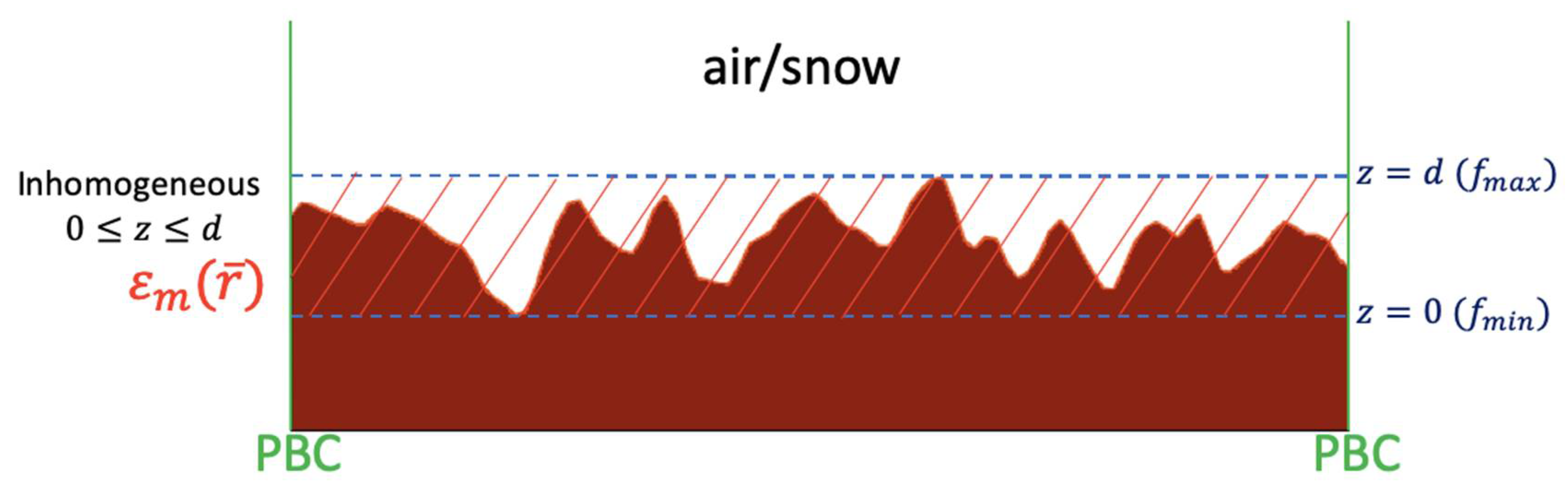
4.1. Formulation of VIE Using Periodic Boundary Conditions and Periodic Half Space Dyadic Green’s Function

We applied the VIE approach with periodic boundary conditions to calculate scattering by a rough soil surface. Since we only consider rough surfaces, the formulation of combined volume and surface scattering in Tan 2016 is simplified [65].
Consider an incident plane wave incident onto a rough surface. The media above and below the rough surface are labeled medium 0 and medium 1 respectively. The permittivities are ε and ε 1 respectively. The wavenumbers are k and k 1 respectively. The medium, 0, can be air or snow with ε =   ε 0 for air and ε =   ε s n o w for snow. The ε 1 in this paper is ε 1 =   ε s o i l for soil. For a single realization of a rough surface (Figure 14) with maximum height f m a x and minimum height f m i n , we set z = 0 at f min and z =   d at f max so that
d = f m a x f m i n
Then, the region 0 z d is an inhomogeneous region. The inhomogeneous permittivity in that region is ε m ( r ¯ ) is
ε m ( r ¯ ) = { ε                       for   r ¯   in   medium   0 ε 1                   for   r ¯   in   medium   1
The region is inhomogeneous, and the problem can be cast into VIE with the surface scattering problem converted into a volume scattering problem in the inhomogeneous region. We discretize the inhomogeneous regions into small cubes that are much smaller than a wavelength. Each small cube has permittivity either ε or ε 1 . Consider an incident plane wave launched from medium 0.
E ¯ i n c ( r ¯ ) = E ¯ 0 e i k i x x + i k i y y + i k i z z
where E ¯ 0 is vertical polarized (TM) or horizontal polarized (TE) and
k i x = k sin θ i cos ϕ i k i y = k sin θ i sin ϕ i k i z = k cos θ i
Let k ¯ i ρ = k i x x ^ + k i y y ^ be the horizontal component of the incident wave vector. Because we use the half space dyadic Green’s function as the background with the rough surface creating the inhomogeneous medium, there is a specular reflected wave when the rough surface is planar, which comes from reflection of a planar surface between medium 0 and medium 1 due to the planar surface at z = 0 .
E ¯ r e f ( r ¯ ) = E ¯ 0 R ( θ ) e i k i x x + i k i y y + i k i z z
where R ( θ ) is the Fresnel reflection coefficient at angle θ i . The reflection coefficient is R ( θ i ) = R T M ( θ i ) for TM and R ( θ i ) = R T E ( θ i ) for TE. By periodic boundary conditions, we mean that the horizontal domain is divided into periodic regions and the permittivities are repeated periodically. The (0,0) period is
L x 2 x L x 2 L y 2 y L y 2
Then, the cells are labeled by integers p , q with p, q = 0, ±1, ±2, … Let
ρ ¯ p q = p L x x ^ + q L y y ^
The periodic permittivities are
ε m ( r ¯ + ρ ¯ p q ) = ε m ( r ¯ )
The boundary value problem is 3D electromagnetic wave scattering, and the periodicity is 2D (labeled as a 3D2D problem). The electric field obeys the Bloch condition
E ¯ ( r ¯ + ρ ¯ p q ) = E ¯ ( r ¯ ) e i k ¯ i ρ · ρ ¯ p q
By making use of periodic Green’s functions, The VIE is converted into one period (0,0) for the inhomogeneous region
E ¯ ( r ¯ ) = E ¯ i n c ( r ¯ ) + k 2 0 d d z L x 2 L x 2 d x L y 2 L y 2 d y G = P ( r ¯ , r ¯ , k ¯ i ρ )   ( ε m ( r ¯ ) ε 1 ) E ¯ ( r ¯ ) ; L x 2 x L x 2 , L y 2 y L y 2 , 0 z d
where r ¯ and r ¯ are in the inhomogeneous region of period (0,0). The G = P ( r ¯ , r ¯ , k ¯ i ρ ) is the half space periodic Dyadic Green’s function. It is decomposed into the free space part G = P ( 0 ) and the reflection part G = P ( R ) .
G = P ( r ¯ , r ¯ , k ¯ i ρ ) = G = P ( 0 ) ( r ¯ , r ¯ , k ¯ i ρ ) + G = P ( R ) ( r ¯ , r ¯ , k ¯ i ρ )
By applying the discrete dipole approximation (DDA) with small cube size Δ V and taking into account the singularity of the dyadic Green’s function of the free space response G = P ( 0 ) ( r ¯ , r ¯ , k ¯ i ρ ) , we obtain the matrix equation.
p ¯ i = α = i [ E ¯ i n c ( r ¯ i ) + E ¯ r e f ( r ¯ i ) + k 2 ε j i   G = P ( 0 ) ( r ¯ , r ¯ , k ¯ i ρ ) · p ¯ j + k 2 ε j   G = P ( R ) ( r ¯ , r ¯ , k ¯ i ρ ) · p ¯ j ]
where
p ¯ i = Δ V ε ( ε m ( r ¯ i ) ε 1 ) E ¯ ( r ¯ i )
is the polarization of the cube.
α = i = Δ V ε ( ε m ( r ¯ i ) ε 1 ) [ I = k 2 ( ε m ( r ¯ i ) ε 1 ) S = ] 1
is the polarizability of the i-th cube and S = is the singular integral over the self cube.
S = = V C ( 0 ) G = P ( 0 ) ( 0 ¯ , r ¯ , k ¯ i ρ ) d r ¯
The expression for half space dyadic Green’s functions are the non-periodic ones in Tsang et al. volume 1 with the wave vectors replaced by Bloch vectors [28]. The free space part is
G = P ( 0 ) ( r ¯ , r ¯ , k ¯ i ρ ) = i 2 Ω α 1 k z α [ e ^ α ( k z α ) e ^ α ( k z α ) + h ^ α ( k z α ) h ^ α ( k z α ) ] e i k ¯ ρ · ( r ¯ r ¯ )                             f o r   z > z
G = P ( 0 ) ( r ¯ , r ¯ , k ¯ i ρ ) = i 2 Ω α 1 k z α [ e ^ α ( k z α ) e ^ α ( k z α ) + h ^ α ( k z α ) h ^ α ( k z α ) ] e i K ¯ ρ · ( r ¯ r ¯ )               f o r   z < z
and the reflected part is
G = P ( R ) ( r ¯ , r ¯ , k ¯ i ρ ) = i 2 Ω α 1 k z α [ R T E e ^ α ( k z α ) e ^ α ( k z α ) + R T M h ^ α ( k z α ) h ^ α ( k z α ) ] e i k ¯ ρ · ( r ¯ ) e i K ¯ ρ · r ¯               f o r   z < z
where k ¯ ρ and K ¯ ρ are respectively the upward Bloch vector and downward Bloch vector.
For 2D periodicity,   Ω = L x L y , the reciprocal lattice vectors are
K ¯ m n = m 2 π L x x ^ + n 2 π L y y ^
where m , n = 0 , ± 1 , ± 2 , . The Bloch vectors are
k ¯ i m n = k ¯ i ρ + K ¯ m n
so that
k z m n = k 2 | k ¯ i m n | 2
We also use α to represent the double index ( m , n ) so that α = m , n   , k z α = k z m n .
The upward propagation Bloch vector is
k ¯ α = k ¯ i m n + k ¯ z m n z ^  
The downward propagation Bloch vector is
K ¯ α = k ¯ i m n k ¯ z m n z ^
The definitions of TE and TM polarization vector e ^ and h ^ follow that of Tsang et al. volume 1 and are
e ^ α ( k z α ) = e ^ α ( k z α ) = 1 | k ¯ i m n | ( k y α x ^ k x α y ^ )
h ^ α ( k z α ) = k z α k | k ¯ i m n | ( k x α x ^ + k y α y ^ ) + | k ¯ i m n | k z ^

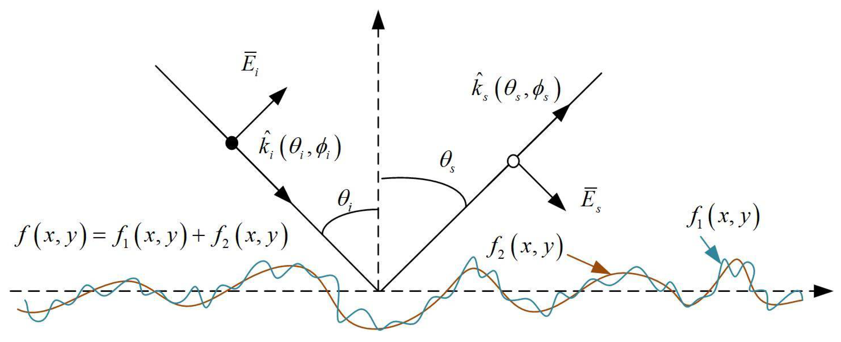
4.2. Modeling and Estimation of the Roughness

In NASA’s Soil Moisture Active Passive (SMAP) mission, the objective is to retrieve soil moisture globally using radar and radiometer observations. For the radar retrieval part, the lookup table (LUT) is applied according to landcover and vegetation type [52]. Kim et al. applied a time-series approach to retrieve soil moisture [29]. For a given pixel, the rms height is assumed constant, so it is not only retrieving soil moisture but also rms height [29]. The retrieved soil moisture and rms height are provided in SMAP L3 Radar Global Daily 3 km EASE-Grid Soil Moisture products through the National Snow & Ice Data Center (NSIDC) [66]. Although SMAP’s radar was only active for 3 months, the amount of retrieved global rms height map provides the basis for our analysis here. Figure 15a plots the rms heights obtained over North America based on the average of rms height maps from the 3 months products. The Figure shows most locations to have rms heights of 2 cm or less while mountainous regions show rms heights from 4 to 6 cm. A histogram of these rms heights for North America is further provided in Figure 15b. In rough-surface scattering at the Ku-band, a upper limit of k h = 2 or 3 was used, which missed the fact that the k h upper limit is actually 20, which is ten times larger than k h = 2. Next, we consider the scattering problem taking into account those fine features at higher frequency.
Consider an incident plane wave on a rough surface as shown in Figure 16. The direction of the incident wave is k ¯ i = k k ^ i = k i x x ^ + k i y y ^ k i z z ^ , where k i x = k   sin θ i cos ϕ i , k i y = k sin θ i sin ϕ i , and k i z = k cos θ i . θ i and ϕ i are the incident elevation and azimuth angle, respectively. The scattered wave E ¯ s is with scattered direction of k ¯ s = k k ^ s = k s x x ^ + k s y y ^ + k s z z ^ , where k s x = k sin θ s cos ϕ s , k s y = k sin θ s sin ϕ s , and k s z = k cos θ s . θ s and ϕ s are the scattering elevation and azimuth angle, respectively.
The roughness profile f ( x , y ) is given by
f ( x , y ) = f 1 ( x , y ) + f 2 ( x , y ) h = h 1 2 + h 2 2 h 2 C ( ρ ) = h 1 2 C 1 ( ρ ) + h 2 2 C 2 ( ρ )
where f 1 ( x , y ) is the finer roughness in millimeter scale with rms height h 1 , correlation length l 1 , and correlation function C 1 ( ρ ) . The f 2 ( x , y ) is roughness in centimeters with rms height h 2 , correlation length l 2 , and correlation function C 2 ( ρ ) . For the combined f 1 ( x , y ) and f 2 ( x , y ) in f ( x , y ) , the rms height h and correlation function C ( ρ ) are given by Equation (141). l is the correlation length of f ( x , y ) that C ( l ) = e x p ( 1 ) .
Figure 17 plots the exponential term of the Kirchoff integral in the backscattering direction as a function of ρ from the L- to the Ku-band. Results indicate that the exponential term has effects on backscatter for ρ more than 10 cm for the L-band. For frequencies above the X-band, the exponential term has effects for ρ less than 3 cm, which is less than the correlation length of f 2 but comparable with the correlation length of f 1 . The millimeter-scale roughness f 1 has effects for high frequency. To investigate the scattering of rough surfaces at the X- and Ku-bands, it is important to include fine-scale roughness f 1 superimposed on f 2 , providing a two-scale roughness for the present simulations.
In the VIE-NMM3D approach, we modeled the rough-surface scattering using a Monte Carlo simulation in which the scattering from each surface realization was computed using a discrete dipole approximation (DDA) to the volume integral [67,68,69].
The rough surface realizations generated are stationary Gaussian random processes having horizontal dimensions L × L . For each realization, the minimum of the rough surface profile, f m i n = M I N { f ( x , y ) } , is defined as z = 0 , and the “depth” of the simulation domain must satisfy d > f m a x f m i n , where f m a x = M A X { f ( x , y ) } . Note this definition of the coordinate system results in a mean surface height > 0 and results in phase offsets for each realization. This is immaterial for the purposes of this work because only the incoherent backscattering coefficient γ ( θ s , ϕ s ) at oblique incidence is examined. The DDA simulation domain of dimension L × L × d is then discretized into small cubes whose dimensions are small compared with the wavelengths of interest and to the roughness scales of interest. Cubes within the soil region are modeled as having the permittivity of soil while those in free space are modeled as having the permittivity of free space. Because these cubes exist in the presence of the soil half space z < 0, a half space Green’s function was used to compute the radiation from each cube with z = 0 representing the half space interface. Periodic boundary conditions were also applied in both horizontal directions to reduce the effect of the horizontal boundaries. This has the effect of discretizing the scattered field into a set of Floquet mode plane waves. However, it should be expected that surface periods L much greater than the wavelengths of interest will produce Floquet mode amplitudes that approximate the scattering in those directions of an infinite continuous rough surface when observed in the same scattering direction.

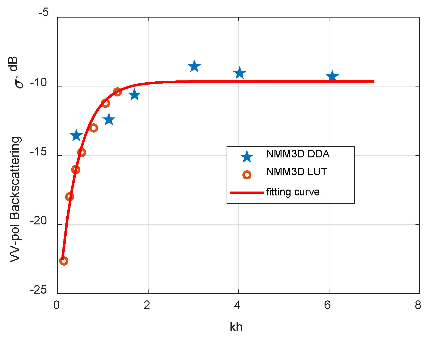
4.3. The Frequency and Roughness Responses of the Backscattering from the Rough Surface

In this section, we provide a few simulation results [46]. More simulation results can be found in the PhD thesis of Jiyue Zhu [47]. In Figure 18, the backscattering is plotted as a function of kh up to kh = 6. The ratio of correlation length to rms height was 7. The simulated frequency was 9.6 GHz. Figure 18 shows that the DDA simulations are in good agreement with previous MoM full-wave simulations LUT up to kh = 1.5 [70]. The backscattering of DDA simulations first increased with kh and then saturated around kh = 2.5. The physical basis behind such phenomena is that the magnitude of waves reflected back to the backscattering direction increase with the roughness and then finally reaches a maximum value (which is corresponding to the geometric optics (GO) realm [39]). Saturation was also postulated by Oh’s empirical model without experimental data in the large kh regime [59].
In Figure 19, the backscattering is plotted as a function of k h for rough surfaces with “limited correlation lengths”. The rms heights (0.3 cm, 0.6 cm, 0.9 cm, 1.2 cm, 1.5 cm, and 1.8 cm) and correlation lengths (2.64 cm, 5.04 cm, 5.85 cm, 6.3 cm, 6.75 cm, and 7.2 cm) are from field measurements in San Luis Valley (SLV), CO, USA. A laser range finder mounted on a horizontal bubble level supported by a tripod at each end was used to measure small-scale surface roughness along the 1 m baseline of the level at multiple locations [42]. The simulated frequency was 13.6 GHz. We considered a snow-covered, rough soil surface. Backscattering first increased with k h to reach the peak around k h = 2.1 and then decreased. Such a decrease is caused by the decrease of the ratio of correlation length and rms height. In the GO limit, smaller ratio yields a weaker backscatter.
In Figure 20, we show the VV backscattering as a function of rms heights at C-, X-, and Ku-bands. The figures show saturation effects, meaning that rough-surface scattering saturates at large rms heights (~3–6 cm) and at high frequencies. The new results of k h up to 15 are useful for studying rough surface radar backscattering at the X- and Ku- bands for snow/soil interfaces.

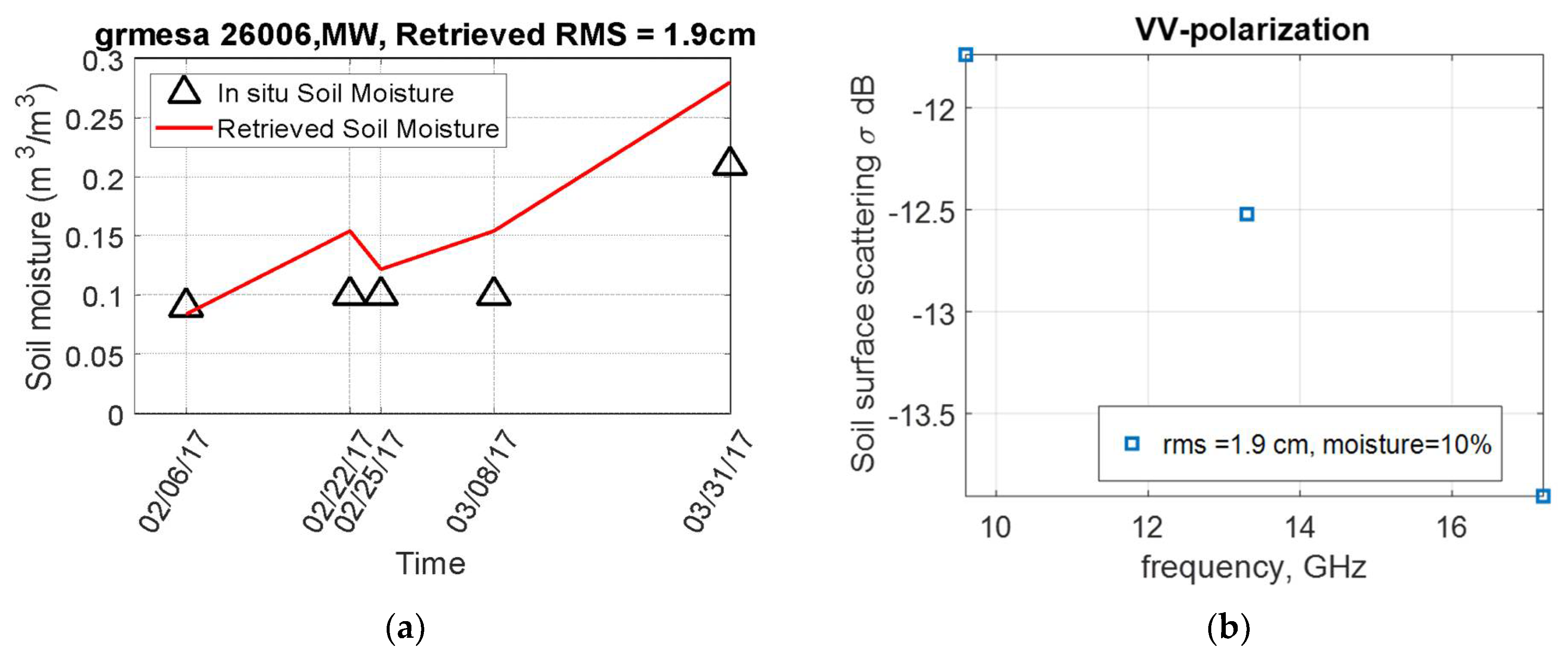
4.4. Using the Retrieved rms Height from UAVSAR L-Band Data to Simulate Backscattering at X- and Ku-Bands

Interaction of Radar Waves with the Ground Surface Beneath the Snowpack

Figure 21 shows radar backscattering from a snow layer. The interaction of radar with snow overlying a rough soil surface involves refraction and scattering from the air/snow interface. In Figure 21, we show the incident plane wave at incident angle θ i . Based on Snell’s law, the transmitted angle is θ t so that the incident angle on the rough soil surface is θ t . With snow relative permittivity of approximately 1.44, the refracted angle θ t was 32.4 degrees, which corresponds to the 40 degrees incidence angle of θ i in air. Because of the magnitude of dielectric contrasts, the contributions of rough-surface scattering are from the snow–soil rough interface and not from the air/snow interface. The air/snow interface has stronger scattering contribution for wet snow which is outside the domain of the X-band and Ku-band volume scattering approach for SWE retrieval.
The volume scattering method at the X-band the and Ku-band has been proposed to retrieve SWE for dry snow. For such a case, the rough surface contribution arises from the rough snow–soil surface below the snow layer. It is proposed in this paper that L-band and C-band radar signals can be used to retrieve both the rms height and the moisture of the soil. Since microwave scattering depends on permittivity. The retrieval of soil moisture covers the various soil conditions of soil texture, freeze–thaw, etc. For wet snow, a rough-surface contribution arises from the air/snow surface. However, the volume scattering method is not proposed for wet snow.
Rough-surface scattering from the snow/soil interface contributes to radar observations as represented by σ r s e x p ( 2 τ s e c θ t ) . The term is affected by the rough soil-surface scattering σ r s and the attenuation through snow factor of e x p ( 2 τ s e c θ t ) . σ refers to either VV or HH. r s stands for rough surface and τ is optical thickness. The rough soil-surface scattering contribution is not related to SWE and it should be removed when retrieving SWE. The subtraction of surface scattering has been used to improve the accuracy of SWE retrieval [17,24]. The approach of removing σ r s e x p ( 2 τ s e c θ t ) consists of using a combination of data and electromagnetic models. The removal of surface scattering is a significant part of the retrieval algorithm that is discussed later in this section.
To estimate rough-surface scattering at the X-band and Ku-band, there are two approaches, (a) and (b). Approach (a) is as described in ref. [18]. In approach (a), radar observations at the X- and Ku-bands at a specific location before the snowfall are used to estimate the surface backscattering [18]. Such an approach neglects changes in soil properties and background land-cover during the snow-on season. In approach (b), the estimation of rough-surface scattering, σ r s , at the X-band and Ku-band consists of using a combination of measurement data and electromagnetic models. The measurement data include backscattering data at the L-band, C-band, X-band and Ku-band before and after snow. The electromagnetic model of rough-surface scattering results is based on using look-up table (LUT) results of Numerical Maxwell 3D model of full-wave simulations of surface scattering from the L-band to the Ku-band. In this section, we illustrate approach (b) using L band UAVSAR data. We used a two-step procedure. In the first step of approach (b), we used co-polarized radar time series observations at the L- and C-bands, which have much larger surface scattering than volume scattering, to estimate soil permittivity and surface roughness. The use of the C-band time series together with the L-band time series enhances the existing L-band algorithm in retrieving rms height and soil moisture. Using L-band and C-band data before and after snow fall together with LUT of Maxwell equations for the L-band and C-band, we retrieve the rough surface rms heights and soil moistures. The retrieval is carried out for both before snow fall and after snow fall. After snow fall, Snell’s law is used to adjust the incident angle at the snow–soil interface to account for the refraction angle at the air/snow interface. In step 2 of approach (b), the rms heights and soil permittivities retrieved in step 1 are used in the NMM3D LUT to obtain the model backscattering results of σ r s at the X- and Ku-bands for the same roughness and soil moisture parameters. Approach (b) is applicable even when there are changes of rms heights and soil moistures during the snow season. Approach (b) assumes the availability of matchup spaceborne L- and/or C-band SAR observations with revisits of 10 days. The revisits provided by the Sentinel-1 and NISAR systems, as well as future proposed continuation missions, suggest that such datasets are likely to be available during the time frame of a future snow observing mission.
We next give an example of approach (b) using UAVSAR L band data to demonstrate the retrieval of rms heights and soil permittivity. We consider, as in step 1, using L-band UAVSAR radar full polarization observations under snow-on conditions using the NMM3D LUT [27]. The UAVSAR dataset was collected from February to March in 2017, in the SnowEx 2017 campaign using five flights over the Grand Mesa region in Colorado, United States. In situ soil moisture measurements were also collected throughout 2017 from an installed meteorological observation station. We apply the time series retrieval algorithm developed for the SMAP mission at the station location, that is, at the point-scale [52,56]. From the retrieved soil permittivity, the soil moisture was derived using Mironov’s empirical model [57]. The comparison of retrieved and measured soil moisture is shown in Figure 22a. In addition to retrieving soil moisture, the rms height was also retrieved from the time series and was at a single value of 1.9 cm. The cost function for retrieving soil moisture and rms height is as follows. By using the L-band rough surface lookup table, we used VV and HH to find the minimum cost function against the observed backscatters. The rms height and time series soil moisture were retrieved at the same time. The retrieved rms height from L-band is assumed to be invariant with time and subsequently can be applied for rough-surface scattering at higher frequencies.
C m i n = m i n { n [ ( σ V V L U T ( h , ϵ n ) σ V V o b s ) 2 + ( σ H H L U T ( h , ϵ n ) σ H H o b s ) 2 ] }
The above description is the rationale of the Kim et al., 2017, algorithm showing that soil moisture changes but not rms height. Wet and frozen soils are assumed to have the same rms height [52].
The retrieval soil moisture is in good agreement, as shown in Figure 22a, with the measured in situ soil moisture for a period of 8 weeks from 6 February 2017 to 31 March 2017. The agreement achieved has a root mean square error (RMSE) of 0.047 m 3 / m 3 , a correlation of 0.95, and a bias of 0.039 m 3 / m 3 . Based on the measurements, the soil moistures at this site were relatively constant during the dry snow season (6 February to 8 March 2017).
To complete approach (b), we carried out step 2 and applied the retrieved rms height of 1.9 cm, and soil properties from Figure 22a to calculate the surface scattering contributions with snow attenuation, σ r s e x p ( 2 τ s e c θ t ) , at the X band of 9.6 GHz, the low Ku band of 13.4 Ghz, and the high Ku-band of 17.2 Ghz. These three frequencies were considered for the proposed satellite snow water equivalent (SWE) missions. Figure 22b shows surface scattering including snow attenuation. The results in Figure 22b show that the rough soil-surface scattering contribution, including snow attenuation, was around −12 dB at the X band and decreased to −14 dB at the high Ku band of 17.2 GHz. Higher frequencies such as at the Ku band typically experience higher volume scattering and greater attenuation from the snow layer of the surface scattering contributions. Continued studies are required to improve and validate the approach (b). These studies include extending NMM3D surface modeling studies and LUT into cases with rms heights of four wavelengths or more so that the LUTs can be applied to the Ku-band of 17.2 GHz up to 7 cm of rms heights. Unlike volume scattering of snow, rough-surface scattering has a stronger dependence on incidence angle. Thus, the effects of topographical slopes that cause changes in incidence angles, particularly in mountainous regions, should be included in the retrieval. The sample size in Figure 22a,b is small. However, with the availability of L band and C band data, full-wave simulations of rough soil-surface scattering from the L band to the Ku band up to k h = 15 allow retrievals of rms heights of the soil surfaces and the soil-surface scattering at the X band and Ku band can be determined.
Our current work is computing look-up tables for rough soil-surface scattering for kh up to 15. We are also continuing investigating various CEM techniques of rough-surface scattering in the large kh domain.

5. Conclusions

In this paper, we reviewed our recent work in three topics of the theory of microwave remote sensing. The effects of vegetation and forests are important topics of microwave remote sensing of soil moisture and the snow water equivalent. The hybrid method of full-wave simulations showed results that are significantly different from that of RTE and DBA. As remote sensing of soil moisture extends from the P-band to the X-band while remote sensing of snow water equivalent covers the P-band to the Ku-band, such studies using full-wave simulations will provide new solutions different from that of RTE/DBA. Signals of opportunity offer new efficient ways of remote sensing at P-band and L-band. The theory of microwave remote sensing at bistatic scattering close to the specular direction requires modeling techniques different from radar backscattering and radiometry. For remote sensing of land surfaces at high frequencies, such as the X-band Ku-band, the theory of microwave remote sensing full-wave simulations needs to be carried out to much larger kh values than before. The study of multiscale surfaces and their effects at large kh continue to be a challenge.

Author Contributions

L.T. contributed to Section 1, Section 2, Section 3, Section 4 and Section 5. T.-H.L. and J.Z. contributed to Section 4. R.G. and W.G. contributed to Section 2. H.X. contributed to Section 3. All authors have read and agreed to the published version of the manuscript.

Funding

The research support for this paper were from the NASA Terrestrial Hydrology Program, the NASA Remote Sensing Theory Program and the NASA CYGNSS Mission.

Conflicts of Interest

The authors declare no conflict of interest.

References

  1. Attema, E.P.W.; Ulaby, F.T. Vegetation modeled as a water cloud. Radio Sci. 1978, 13, 357–364. [Google Scholar] [CrossRef]
  2. Huang, H.; Tsang, L.; Colliander, A.; Yueh, S.H. Propagation of Waves in Randomly Distributed Cylinders Using Three-Dimensional Vector Cylindrical Wave Expansions in Foldy–Lax Equations. IEEE J. Multiscale Multiphysics Comput. Tech. 2019, 4, 214–226. [Google Scholar] [CrossRef]
  3. Huang, H.; Tsang, L.; Colliander, A.; Shah, R.; Xu, X.; Yueh, S. Multiple scattering of waves by complex objects using hybrid method of t-matrix and foldy-lax equations using vector spherical waves and vector spheroidal waves. Prog. Electromagn. Res. 2020, 168, 87–111. [Google Scholar] [CrossRef]
  4. Gu, W.; Tsang, L.; Colliander, A.; Yueh, S.H. Wave Propagation in Vegetation Field Using a Hybrid Method. IEEE Trans. Antennas Propag. 2021, 69, 6752–6761. [Google Scholar] [CrossRef]
  5. Gu, W.; Tsang, L.; Colliander, A.; Yueh, S.H. Multifrequency Full-Wave Simulations of Vegetation Using a Hybrid Method. IEEE Trans. Microw. Theory Tech. 2021, 70, 275–285. [Google Scholar] [CrossRef]
  6. Unwin, M.; Jales, P.; Tye, J.; Gommenginger, C.; Foti, G.; Rosello, J. Spaceborne GNSS-Reflectometry on TechDemoSat-1: Early Mission Operations and Exploitation. IEEE J. Sel. Top. Appl. Earth Obs. Remote Sens. 2016, 9, 4525–4539. [Google Scholar] [CrossRef]
  7. Ruf, C.; Unwin, M.; Dickinson, J.; Rose, R.; Rose, D.; Vincent, M.; Lyons, A. CYGNSS: Enabling the Future of Hurricane Prediction [Remote Sensing Satellites]. IEEE Geosci. Remote Sens. Mag. 2013, 1, 52–67. [Google Scholar] [CrossRef]
  8. Kim, H.; Lakshmi, V. Use of Cyclone Global Navigation Satellite System (CyGNSS) Observations for Estimation of Soil Moisture. Geophys. Res. Lett. 2018, 45, 8272–8282. [Google Scholar] [CrossRef] [Green Version]
  9. Chew, C.C.; Small, E.E. Soil Moisture Sensing Using Spaceborne GNSS Reflections: Comparison of CYGNSS Reflectivity to SMAP Soil Moisture. Geophys. Res. Lett. 2018, 45, 4049–4057. [Google Scholar] [CrossRef] [Green Version]
  10. Clarizia, M.P.; Pierdicca, N.; Costantini, F.; Floury, N. Analysis of CYGNSS Data for Soil Moisture Retrieval. IEEE J. Sel. Top. Appl. Earth Obs. Remote Sens. 2019, 12, 2227–2235. [Google Scholar] [CrossRef]
  11. Shah, R.; Xu, X.; Yueh, S.; Chae, C.S.; Elder, K.; Starr, B.; Kim, Y. Remote Sensing of Snow Water Equivalent Using P-Band Coherent Reflection. IEEE Geosci. Remote Sens. Lett. 2017, 14, 309–313. [Google Scholar] [CrossRef]
  12. Yueh, S.H.; Shah, R.; Xu, X.; Stiles, B.; Bosch-Lluis, X. A Satellite Synthetic Aperture Radar Concept Using P-Band Signals of Opportunity. IEEE J. Sel. Top. Appl. Earth Obs. Remote Sens. 2021, 14, 2796–2816. [Google Scholar] [CrossRef]
  13. Gu, W.; Xu, H.; Tsang, L. A numerical kirchhoff simulator for gnss-r land applications. Prog. Electromagn. Res. 2019, 164, 119–133. [Google Scholar] [CrossRef] [Green Version]
  14. Zhu, J.; Tsang, L.; Xu, H. A physical patch model for gnss-r land applications. Prog. Electromagn. Res. 2019, 165, 93–105. [Google Scholar] [CrossRef] [Green Version]
  15. Xu, H.; Zhu, J.; Tsang, L.; Kim, A.S.B. A fine scale partially coherent patch model including topographical effects for gnss-r ddm simulations. Prog. Electromagn. Res. 2021, 170, 97–128. [Google Scholar] [CrossRef]
  16. Ren, B.; Zhu, J.; Tsang, L.; Xu, A.H. Analytical Kirchhoff Solutions (Aks) and Numerical Kirchhoff Approach (Nka) for First-Principle Calculations of Coherent Waves and Incoherent Waves at P Band and L Band in Signals of Opportunity (Soop). Prog. Electromagn. Res. 2021, 171, 35–73. [Google Scholar] [CrossRef]
  17. Tsang, L.; Durand, M.; Derksen, C.; Barros, A.P.; Kang, D.H.; Lievens, H.; Marshall, H.P.; Zhu, J.; Johnson, J.; King, J.; et al. Review Article: Global Monitoring of Snow Water Equivalent Using High Frequency Radar Remote Sensing. The Cryosphere 2022. accepted. [Google Scholar] [CrossRef]
  18. Rott, H.; Yueh, S.H.; Cline, D.W.; Duguay, C.; Essery, R.; Haas, C.; Hélière, F.; Kern, M.; Macelloni, G.; Malnes, E.; et al. Cold Regions Hydrology High-Resolution Observatory for Snow and Cold Land Processes. Proc. IEEE 2010, 98, 752–765. [Google Scholar] [CrossRef] [Green Version]
  19. Lemmetyinen, J.; Derksen, C.; Rott, H.; Macelloni, G.; King, J.; Schneebeli, M.; Wiesmann, A.; Leppänen, L.; Kontu, A.; Pulliainen, J. Retrieval of Effective Correlation Length and Snow Water Equivalent from Radar and Passive Microwave Measurements. Remote Sens. 2018, 10, 170. [Google Scholar] [CrossRef] [Green Version]
  20. King, J.; Derksen, C.; Toose, P.; Langlois, A.; Larsen, C.; Lemmetyinen, J.; Marsh, P.; Montpetit, B.; Roy, A.; Rutter, N.; et al. The influence of snow microstructure on dual-frequency radar measurements in a tundra environment. Remote Sens. Environ. 2018, 215, 242–254. [Google Scholar] [CrossRef]
  21. Xiong, C.; Shi, J.; Pan, J.; Xu, H.; Che, T.; Zhao, T.; Ren, Y.; Geng, D.; Jiang, K.; Feng, P. Time Series X- and Ku-Band Ground-Based Synthetic Aperture Radar Observation of Snow-Covered Soil and Its Electromagnetic Modeling. IEEE Trans. Geosci. Remote Sens. 2021, 60, 1–13. [Google Scholar] [CrossRef]
  22. Tan, S.; Chang, W.; Tsang, L.; Lemmetyinen, J.; Proksch, M. Modeling Both Active and Passive Microwave Remote Sensing of Snow Using Dense Media Radiative Transfer (DMRT) Theory with Multiple Scattering and Backscattering Enhancement. IEEE J. Sel. Top. Appl. Earth Obs. Remote Sens. 2015, 8, 4418–4430. [Google Scholar] [CrossRef]
  23. Tsang, L.; Tan, S.; Xiong, C.; Shi, J. 4.05—Optical and Microwave Modeling of Snow. In Comprehensive Remote Sensing; Liang, S., Ed.; Elsevier: Oxford, UK, 2018; pp. 85–138. ISBN 978-0-12-803221-3. [Google Scholar]
  24. Zhu, J.; Tan, S.; King, J.; Derksen, C.; Lemmetyinen, J.; Tsang, L. Forward and Inverse Radar Modeling of Terrestrial Snow Using SnowSAR Data. IEEE Trans. Geosci. Remote Sens. 2018, 56, 7122–7132. [Google Scholar] [CrossRef]
  25. Huang, S.; Tsang, L.; Njoku, E.G.; Chan, K.S. Backscattering Coefficients, Coherent Reflectivities, and Emissivities of Randomly Rough Soil Surfaces at L-Band for SMAP Applications Based on Numerical Solutions of Maxwell Equations in Three-Dimensional Simulations. IEEE Trans. Geosci. Remote Sens. 2010, 48, 2557–2568. [Google Scholar] [CrossRef]
  26. Huang, S.; Tsang, L. Electromagnetic Scattering of Randomly Rough Soil Surfaces Based on Numerical Solutions of Maxwell Equations in Three-Dimensional Simulations Using a Hybrid UV/PBTG/SMCG Method. IEEE Trans. Geosci. Remote Sens. 2012, 50, 4025–4035. [Google Scholar] [CrossRef]
  27. Liao, T.-H.; Tsang, L.; Huang, S.; Niamsuwan, N.; Jaruwatanadilok, S.; Kim, S.-B.; Ren, H.; Chen, K.-L. Copolarized and Cross-Polarized Backscattering from Random Rough Soil Surfaces from L-Band to Ku-Band Using Numerical Solutions of Maxwell’s Equations with Near-Field Precondition. IEEE Trans. Geosci. Remote Sens. 2015, 54, 651–662. [Google Scholar] [CrossRef]
  28. Tsang, L.; Kong, J.A.; Ding, K.-H. Scattering of Electromagnetic Waves: Theories and Applications; John Wiley & Sons, Inc.: New York, NY, USA, 2000; Volume 1, ISBN 978-0-471-22428-0. [Google Scholar]
  29. Kim, S.-B.; Moghaddam, M.; Tsang, L.; Burgin, M.; Xu, X.; Njoku, E.G. Models of L-Band Radar Backscattering Coefficients Over Global Terrain for Soil Moisture Retrieval. IEEE Trans. Geosci. Remote Sens. 2013, 52, 1381–1396. [Google Scholar] [CrossRef]
  30. Huang, H.; Liao, T.-H.; Kim, S.B.; Xu, X.; Tsang, L.; Jackson, T.J.; Yueh, A.S. L-Band radar scattering and soil moisture retrieval of wheat, canola and pasture fields for smap active algorithms. Prog. Electromagn. Res. 2021, 170, 129–152. [Google Scholar] [CrossRef]
  31. Tsang, L.; Ishimaru, A. Backscattering enhancement of random discrete scatterers. J. Opt. Soc. Am. A 1984, 1, 836–839. [Google Scholar] [CrossRef]
  32. Lang, R.H.; Khadr, N. Effects of Backscattering Enhancement on Soil Moisture Sensitivity. In Proceedings of the IGARSS ’92 International Geoscience and Remote Sensing Symposium, Houston, TX, USA, 26–29 May 1992; Volume 2, pp. 916–919. [Google Scholar]
  33. Liao, T.-H.; Kim, S.-B.; Tan, S.; Tsang, L.; Su, C.; Jackson, T.J. Multiple Scattering Effects with Cyclical Correction in Active Remote Sensing of Vegetated Surface Using Vector Radiative Transfer Theory. IEEE J. Sel. Top. Appl. Earth Obs. Remote Sens. 2016, 9, 1414–1429. [Google Scholar] [CrossRef]
  34. Huang, H.; Tsang, L.; Njoku, E.G.; Colliander, A.; Liao, T.-H.; Ding, K.-H. Propagation and Scattering by a Layer of Randomly Distributed Dielectric Cylinders Using Monte Carlo Simulations of 3D Maxwell Equations with Applications in Microwave Interactions with Vegetation. IEEE Access 2017, 5, 11985–12003. [Google Scholar] [CrossRef]
  35. Jing, C.; Niu, X.; Duan, C.; Lu, F.; Di, G.; Yang, X. Sea Surface Wind Speed Retrieval from the First Chinese GNSS-R Mission: Technique and Preliminary Results. Remote Sens. 2019, 11, 3013. [Google Scholar] [CrossRef] [Green Version]
  36. Clarizia, M.P.; Ruf, C.S. Wind Speed Retrieval Algorithm for the Cyclone Global Navigation Satellite System (CYGNSS) Mission. IEEE Trans. Geosci. Remote Sens. 2016, 54, 4419–4432. [Google Scholar] [CrossRef]
  37. Li, W.; Cardellach, E.; Fabra, F.; Rius, A.; Ribó, S.; Martín-Neira, M. First spaceborne phase altimetry over sea ice using TechDemoSat-1 GNSS-R signals. Geophys. Res. Lett. 2017, 44, 8369–8376. [Google Scholar] [CrossRef]
  38. Nghiem, S.V.; Zuffada, C.; Shah, R.; Chew, C.; Lowe, S.T.; Mannucci, A.J.; Cardellach, E.; Brakenridge, G.; Geller, G.; Rosenqvist, A. Wetland monitoring with Global Navigation Satellite System reflectometry. Earth Space Sci. 2016, 4, 16–39. [Google Scholar] [CrossRef]
  39. Tsang, L.; Kong, J.A. Scattering of Electromagnetic Waves: Advanced Topics; John Wiley & Sons, Inc.: New York, NY, USA, 2001; Volume 3, ISBN 978-0-471-22427-3. [Google Scholar]
  40. Zavorotny, V.; Voronovich, A. Scattering of GPS signals from the ocean with wind remote sensing application. IEEE Trans. Geosci. Remote Sens. 2000, 38, 951–964. [Google Scholar] [CrossRef] [Green Version]
  41. Campbell, J.D.; Melebari, A.; Moghaddam, M. Modeling the Effects of Topography on Delay-Doppler Maps. IEEE J. Sel. Top. Appl. Earth Obs. Remote Sens. 2020, 13, 1740–1751. [Google Scholar] [CrossRef]
  42. Campbell, J.D.; Akbar, R.; Azemati, A.; Bringer, A.; Comite, D.; Dente, L.; Gleason, S.T.; Guerriero, L.; Hodges, E.; Johnson, J.T.; et al. Intercomparison of Models for CYGNSS Delay-Doppler Maps at a Validation Site in the San Luis Valley of Colorado. In Proceedings of the 2021 IEEE International Geoscience and Remote Sensing Symposium IGARSS, Brussels, Belgium, 11–16 July 2021; pp. 2001–2004. [Google Scholar]
  43. Thompson, D.; Elfouhaily, T.; Garrison, J. An improved geometrical optics model for bistatic GPS scattering from the ocean surface. IEEE Trans. Geosci. Remote Sens. 2005, 43, 2810–2821. [Google Scholar] [CrossRef]
  44. Bringer, A.; Johnson, J.T.; Toth, C.; Ruf, C.; Moghaddam, M. Studies of Terrain Surface Roughness and Its Effect on GNSS-R Systems Using Airborne Lidar Measurements. In Proceedings of the 2021 IEEE International Geoscience and Remote Sensing Symposium IGARSS, Brussels, Belgium, 11–16 July 2021; pp. 2016–2019. [Google Scholar]
  45. Rodriguez, E.; Morris, C.S.; Belz, J.E.; Chapin, E.; Martin, J.; Daffer, W.; Hensley, S. An Assessment of the SRTM Topographic Products; Technical Report JPL D-31639; JPL: Pasadena, CA, USA, 2005. [Google Scholar]
  46. Zhu, J.; Tsang, L.; Liao, T.-H. Scattering from Random Rough Surfaces at X and Ku Band for Global Remote Sensing of Ter-restrial Snow. In Proceedings of the 2021 IEEE International Symposium on Antennas and Propagation and USNC-URSI Radio Science Meeting (APS/URSI), Singapore, 10–16 July 2021; pp. 1115–1116. [Google Scholar]
  47. Zhu, J. Surface and Volume Scattering Model in Microwave Remote Sensing of Snow and Soil Moisture. Ph.D. Thesis, Department of EECS, University of Michigan, Ann Arbor, MI, USA, December 2021. [Google Scholar]
  48. Ishimaru, A. Wave Propagation and Scattering in Random Media; Multiple Scattering, Turbulence, Rough Surfaces, and Remote Sensing; Academic Press: Cambridge, MA, USA, 1978; ISBN 978-0-12-374702-0. [Google Scholar]
  49. Chen, K.S.; Wu, T.D.; Tsang, L.; Li, Q.; Shi, J.C.; Fung, A.K. Emission of rough surfaces calculated by the integral equation method with comparison to three-dimensional moment method simulations. IEEE Trans. Geosci. Remote Sens. 2003, 41, 90–101. [Google Scholar] [CrossRef]
  50. Voronovich, A. Small-slope approximation for electromagnetic wave scattering at a rough interface of two dielectric half-spaces. Waves Random Media 1994, 4, 337–367. [Google Scholar] [CrossRef]
  51. Elfouhaily, T.M.; Johnson, J.T. The Reduced Local Curvature Approximation for Rough Surface Scattering. In Proceedings of the 2007 IEEE International Geoscience and Remote Sensing Symposium, Barcelona, Spain, 23–28 July 2007; pp. 1354–1357. [Google Scholar]
  52. Kim, S.-B.; Van Zyl, J.J.; Johnson, J.T.; Moghaddam, M.; Tsang, L.; Colliander, A.; Dunbar, R.S.; Jackson, T.J.; Jaruwatanadilok, S.; West, R.; et al. Surface Soil Moisture Retrieval Using the L-Band Synthetic Aperture Radar Onboard the Soil Moisture Active–Passive Satellite and Evaluation at Core Validation Sites. IEEE Trans. Geosci. Remote Sens. 2017, 55, 1897–1914. [Google Scholar] [CrossRef] [PubMed]
  53. Ulaby, F.T.; Batlivala, P.P.; Dobson, M.C. Microwave Backscatter Dependence on Surface Roughness, Soil Moisture, and Soil Texture: Part I-Bare Soil. IEEE Trans. Geosci. Electron. 1978, 16, 286–295. [Google Scholar] [CrossRef]
  54. Kay, B.D. Soil Structure and Organic Carbon: A Review. In Soil Processes and the Carbon Cycle; CRC Press: Boca Raton, FL, USA, 1997; ISBN 978-0-203-73927-3. [Google Scholar]
  55. Ulaby, F.T.; Long, D.G. Microwave Radar and Radiometric Remote Sensing; The University of Michigan Press: Ann Arbor, MI, USA, 2014; ISBN 978-0-472-11935-6. [Google Scholar]
  56. Kim, S.-B.; Tsang, L.; Johnson, J.T.; Huang, S.; van Zyl, J.J.; Njoku, E.G. Soil Moisture Retrieval Using Time-Series Radar Observations Over Bare Surfaces. IEEE Trans. Geosci. Remote Sens. 2011, 50, 1853–1863. [Google Scholar] [CrossRef]
  57. Mironov, V.; Dobson, M.; Kaupp, V.; Komarov, S.; Kleshchenko, V. Generalized refractive mixing dielectric model for moist soils. IEEE Trans. Geosci. Remote Sens. 2004, 42, 773–785. [Google Scholar] [CrossRef]
  58. Peplinski, N.R.; Ulaby, F.T.; Dobson, M.C. Dielectric properties of soils in the 0.3–1.3-GHz range. IEEE Trans. Geosci. Remote Sens. 1995, 33, 803–807. [Google Scholar] [CrossRef]
  59. Oh, Y.; Sarabandi, K.; Ulaby, F.T. An empirical model and an inversion technique for radar scattering from bare soil surfaces. IEEE Trans. Geosci. Remote Sens. 1992, 30, 370–381. [Google Scholar] [CrossRef]
  60. Lawrence, H.; Demontoux, F.; Wigneron, J.-P.; Paillou, P.; Wu, T.-D.; Kerr, Y.H. Evaluation of a Numerical Modeling Approach Based on the Finite-Element Method for Calculating the Rough Surface Scattering and Emission of a Soil Layer. IEEE Geosci. Remote Sens. Lett. 2011, 8, 953–957. [Google Scholar] [CrossRef]
  61. Mrnka, M. Random Gaussian Rough Surfaces for Full-Wave Electromagnetic Simulations. In Proceedings of the 2017 Conference on Microwave Techniques (COMITE), Brno, Czech Republic, 20–21 April 2017; pp. 1–4. [Google Scholar]
  62. Wei, Y.-W.; Wang, C.-F.; Kee, C.Y.; Chia, T.-T. An Accurate Model for the Efficient Simulation of Electromagnetic Scattering from an Object Above a Rough Surface with Infinite Extent. IEEE Trans. Antennas Propag. 2020, 69, 1040–1051. [Google Scholar] [CrossRef]
  63. Duan, X.; Moghaddam, M. Bistatic Vector 3-D Scattering from Layered Rough Surfaces Using Stabilized Extended Boundary Condition Method. IEEE Trans. Geosci. Remote Sens. 2012, 51, 2722–2733. [Google Scholar] [CrossRef]
  64. Chen, K.-S.; Tsang, L.; Chen, K.-L.; Liao, T.H.; Lee, J.-S. Polarimetric Simulations of SAR at L-Band Over Bare Soil Using Scattering Matrices of Random Rough Surfaces from Numerical Three-Dimensional Solutions of Maxwell Equations. IEEE Trans. Geosci. Remote Sens. 2014, 52, 7048–7058. [Google Scholar] [CrossRef]
  65. Tan, S.; Xiong, C.; Xu, X.; Tsang, L. Uniaxial Effective Permittivity of Anisotropic Bicontinuous Random Media Using NMM3D. IEEE Geosci. Remote Sens. Lett. 2016, 13, 1168–1172. [Google Scholar] [CrossRef]
  66. Kim, S.; Van Zyl, J.; Dunbar, R.S.; Njoku, E.G.; Johnson, J.T.; Moghaddam, M.; Tsang, L. SMAP L3 Radar Global Daily 3 km EASE-Grid Soil Moisture, Version 3; NASA National Snow and Ice Data Center Distributed Active Archive Center: Boulder, CO, USA, 2016. [Google Scholar] [CrossRef]
  67. Tan, S.; Zhu, J.; Tsang, L.; Nghiem, S.V. Microwave Signatures of Snow Cover Using Numerical Maxwell Equations Based on Discrete Dipole Approximation in Bicontinuous Media and Half-Space Dyadic Green’s Function. IEEE J. Sel. Top. Appl. Earth Obs. Remote Sens. 2017, 10, 4686–4702. [Google Scholar] [CrossRef]
  68. Tan, S. Multiple Volume Scattering in Random Media and Periodic Structures with Applications in Microwave Remote Sensing and Wave Functional Materials. Ph.D. Thesis, University of Michigan, Ann Arbor, MI, USA, 2016. [Google Scholar]
  69. Tsang, L.; Kong, J.A.; Ding, K.-H.; Ao, C.O. Scattering of Electromagnetic Waves: Numerical Simulations; John Wiley & Sons, Inc.: New York, NY, USA, 2001; Volume 2, ISBN 978-0-471-22430-3. [Google Scholar]
  70. Wu, T.-D.; Chen, K.-S.; Shi, J.C.; Lee, H.-W.; Fung, A.K. A Study of an AIEM Model for Bistatic Scattering from Randomly Rough Surfaces. IEEE Trans. Geosci. Remote Sens. 2008, 46, 2584–2598. [Google Scholar] [CrossRef]
Figure 1. Single corn plant geometry.
Remotesensing 14 03640 g001
Figure 2. Quasi-periodic arrangement of 9 corn plants in the simulation. The displacement is not periodic, Δ d = [ 0 , 0.05 d ] where d = 0.85 m.
Remotesensing 14 03640 g002
Figure 3. Plot the f v v versus ϕ s for fixed θ i = 140 ° , ϕ i = 0 ° , and θ s = 140 ° , and N m a x = 6 , n = 0 . (In the FEKO, we simulate 37 points, and in the MATLAB, we interpolate it to 370 points).
Remotesensing 14 03640 g003
Figure 4. Plot the T n 0 N N versus n for fixed θ i = 140 ° , θ s = 140 ° , and N m a x = 6 , n = 0 .
Remotesensing 14 03640 g004
Figure 5. (a) Single corn plant in the simulation, line in (a): x = 2   m , y = 0 , z = 2   m to 2   m ; 35 points for θ s and θ i = 140 ° , ϕ i = 0 ° . (b) Scattered field for a single corn plant as a function of z along the blue line in Figure 5a.
Remotesensing 14 03640 g005
Figure 6. Tree trunks (left) are modelled as dielectric cylinders (right). The Figure is adapted with permission from Ref. [2]. © 2019 IEEE.
Remotesensing 14 03640 g006
Figure 7. (a) Scattering from wheat plants in the radius of the circumscribing cylinder, 6.5 cm; distance between the centers of 2 circumscribing cylinders is r d = 14 cm, the closest distance between 2 circumscribing cylinders is g d = 1 cm. Figure is adapted with permission from Ref. [4]. © 2021 IEEE. (b) Transmission of microwave through wheat predicted by the hybrid method and the RTE vary with vegetation water content (VWC).
Remotesensing 14 03640 g007
Figure 8. Profile of f = f 1 + f 2 + f 3 . f 1 : microwave roughness, f 2 : finescale topography, f 3 : planar from DEM. f 1 and f 2 are random, f 3 is deterministic.
Remotesensing 14 03640 g008
Figure 9. Geometry of GNSS-R for the coherent and incoherent models.
Remotesensing 14 03640 g009
Figure 10. Specifications of the transmitter and receiver, and definitions of patches and wave vectors.
Remotesensing 14 03640 g010
Figure 11. Bistatic scattering coefficient for covariance of fields in the L and P bands with GO, AKS, and IGOM. Results show that AKS has a frequency dependence while GO and IGOM do not.
Remotesensing 14 03640 g011
Figure 12. γ m e a n   f i e l d and γ c o v a r for the L-band and P-band. Results have shown that the NKA has good agreement with AKS. In the P-band, γ m e a n   f i e l d is always much larger than γ c o v a r , while for the L-band, γ c o v a r is much larger than γ m e a n   f i e l d .
Remotesensing 14 03640 g012
Figure 13. Track-wise comparison between AKS and CYGNSS v3.0 data from Physical Oceanography Distributed Active Archive Center (PODAAC).
Remotesensing 14 03640 g013
Figure 14. The illustration of simulation geometry, reference plane, periodic boundary conditions (PBC), and half space boundary.
Remotesensing 14 03640 g014
Figure 15. (a) Averaged rms height map from SMAP L3 SM product over North America and (b) histogram of soil rms height in percentage over North America.
Remotesensing 14 03640 g015
Figure 16. Wave scattering from a rough surface with two roughness scales.
Remotesensing 14 03640 g016
Figure 17. The exponential factor in the Kirchhoff integral, e x p ( k d x 2 h 2 ( 1 C ( ρ ) ) ) e x p ( k d x 2 h 2 ) versus ρ at backscattering direction from the L- to the Ku-band. The rough surface is exponential with parameters of h 1 = 0.3   cm ,     l 1 = 1.2   cm , and h 2 = 2.0   cm ,   l 2 = 14   cm .
Remotesensing 14 03640 g017
Figure 18. Backscattering as a function of k h for rough surfaces with a “constant ratio” of 7. The incident angle is 40 degrees and soil permittivity is 5.5 + 2 i . The stars are DDA simulations. The circles are from previous full-wave simulations [27]. The fitting curve is generated based on NMM3D results.
Remotesensing 14 03640 g018
Figure 19. Backscattering as a function of k h for rough surfaces with “constant correlation length”. The upper medium is snow with permititivy of 1.44 and the lower medium is soil permittivity of 5.5 + 2 i . The red curve is with snow attenuation and blue curve without snow attenuation.
Remotesensing 14 03640 g019
Figure 20. Backscattering at VV-polarization as a function of rms height with soil of 10% moisture at C-, X-, and Ku-bands.
Remotesensing 14 03640 g020
Figure 21. The interaction of radar with snow overlying a rough soil surface.
Remotesensing 14 03640 g021
Figure 22. (a) Retrieval of soil moisture compared with in situ measurements. The retrieved rms height is 1.9 cm. The retrieval is based on based on L-band UAVSAR data from SnowEx 2017 campaign. The measured soil moisture is from SnowEx 2017 campaign meteorological observations with a measured soil temperature of 0.6° C. The location of the station is 39.03388°N, 108.21399°W with an elevation of 3033 m. (b) Simulated surface scattering with snow attenuation from the X- to the Ku-band at VV polarization. Snow parameters have a depth of 54 cm, density of 183 kg m−3, ζ = 1.2 mm, and b = 1.2. Blue marks are based on the SnowEx 2017 campaign data shown in (a).
Remotesensing 14 03640 g022
Table 1. Comparison between CEM method and hybrid method.
CEM MethodHybrid MethodComments
Full WaveEntire problem of Np number of plantsSingle plant is an object. T matrix is obtained for the plantEach plant is an object
In RT: each leaf is an object. Each branch is an object
Field SolutionsN = number of unknowns in field solutions, in millionsMultiple scattering of Np plants
Np moderate number, e.g., 100
NA
ReusableNot reusable, solve N field unknowns for each realizationT matrices of a few plants plus azimuthal α rotations, reused for
(i) configurations, random, quasi-periodic
(ii) realizations
(iii) future use
T matrices put on shelves for future use T matrices Portable
Iteration Solution of Each Realizationlarge number of iterations (e.g., conjugate gradient) for large number of N field unknowns to reach convergence of “exact” field solutionIterate Foldy–Lax to obtain multiple scattering order solutions,
second order, fourth order, tenth order, even orders of solutions
Significant wave iterations within a plant which are included in T matrix of a plant, less wave interactions between plants
For vegetation fields and forests, no more than 10 multiple orders of solutions
Averaging over Realizations to Calculate
Statistical Moments
Averaging “exact” solutions over Nr realizationsAveraging Nr realizations after second order, fourth order, sixth order, until statistical moments convergeAveraged second order solutions, fourth-order solutions, are analogous to analytical random media theory SPM in rough surfaces and iterative solutions of radiative transfer equation
Table 2. The choice of N m a x for different θ or θ i .
θ   or   θ i N m a x 2 N m a x + 1 θ   or   θ i N m a x 2 N m a x + 1
2595.18°613
7.18°25100.35°511
12.35°25105.53°511
17.53°25110.71°511
22.71°37115.88°511
27.88°49121.06°49
33.06°49126.24°49
38.24°49131.41°49
43.41°49136.59°49
48.59°49141.76°49
53.76°49146.94°49
58.94°49152.12°49
64.12°511157.29°37
69.29°511162.47°25
74.47°511167.65°25
79.65°511172.82°25
84.82°613178°25
90°613
Table 3. Transmission coefficient from RTE based on distorted Born approximation (RTE/DBA) and the hybrid method from Figure 6. The table is adapted with permission from Ref. [2]. © 2019 IEEE.
RTE/DBAHybrid Method
Transmission0.350.66
Table 4. Comparison between radar backscattering and GNSS-R.
Radar Backscattering
with 40 Degrees Incident Angle
GNSS-R
Observation Close to Specular Direction
ScatteringLarge angle from specularSmall angle from specular
Kirchhoff integralNot Valid as Kirchhoff predicts VV is comparable to HHAccurate near specular direction
RoughnessMicrowave roughness
Topography have small effects
Topography strong influence
+microwave roughness
Mean field intensity/Covariance of fieldCovariance of fields onlyMean field intensity and Covariance of fields
Gamma/sigma0−25 dB to 0 dBMuch Larger values
10 dB to 30 dB
Table 5. Summary of the two Kirchhoff approaches.
ModelsNumerical Kirchhoff Approach (NKA) [13]Analytical Kirchhoff Solution (AKS) [16]
Discretization2 cm30-m DEM patch
Monte Carlo simulationsMonte Carlo
Speckle fluctuations
Analytical
No Monte Carlo
No fluctuations
CPU time for one DDM pixel of 15 kmIntensive
1 week for one DMM
Fast
1 h for one DDM
f1 and f2 constant
ValidationAccurate benchmark
based on brute force
calculations
Validated by NKA
DEM Coarse f3Planar with slope, deterministicPlanar with slope, deterministic
Fine scale f2: randomMonte Carlo averageAnalytical average
Microwave f1: randomMonte Carlo averageAnalytical average
Combining roughness f = f 1 + f 2 + f 3 f 12 = f 1 + f 2 combined dividing line not needed
Spectrum W(k)Can directly use W(k)Can directly use W(k)
Histogram statistics of amplitude and phaseYesNo
Table 6. Descriptions of f 1 ( x , y ) , f 2 ( x , y ) , and f 12 ( x , y ) .
Scales Microwave   Roughness   f 1 ( x , y ) Fine - Scale   Topography   f 2 ( x , y ) Combined   Profile   f 12 ( x , y )
Correlation Function h 1 2 C 1 ( x , y ) h 2 2 C 2 ( x , y ) h 2 C ( x , y )
Spectrum W 1 ( k x , k y ) W 2 ( k x , k y ) W ( k x , k y )
Table 7. Typical values of the attenuation factor in GO-Att. k = 33   m 1 , θ i = 40 ° .
h 1 ( c m ) 4 k 2 h 1 2 cos 2 θ i e x p ( 4 k 2 h 1 2 cos 2 θ i ) ( d B )
1 0.26 1.11
2 1.02 4.44
3 2.30 10.0
6 6.39 40.0
Table 8. Correlation length l 2 and coarse topography slope.
Longitude l 2   ( Times   of   h 2 ) p 3 2 + q 3 2
<−105.90125/
−105.86690.0599
−105.83530.0785
−105.79520.0797
−105.76500.0837
−105.73610.0679
−105.69830.0503
−105.66740.0569
−105.62930.0448
−105.591260.0331
>−105.56125/
Table 9. kh of 5-cm rms height for air/soil and snow/soil interface from L- to Ku-band.
rms   Height ,   h   =   5   c m L Band
(1.26 GHz)
S Band
(2.5 GHz)
C Band
(5.4 GHz)
X Band
(9.6 GHz)
Low Ku Band (13.6 GHz)High Ku Band (17.2 GHz)
kh, air/soil interface1.322.625.6610.0614.2518.02
kh, snow/soil interface1.583.146.7912.0717.1021.63
Publisher’s Note: MDPI stays neutral with regard to jurisdictional claims in published maps and institutional affiliations.

