A Comprehensive Machine Learning Study to Classify Precipitation Type over Land from Global Precipitation Measurement Microwave Imager (GPM-GMI) Measurements

Abstract

Precipitation type is a key parameter used for better retrieval of precipitation characteristics as well as to understand the cloud–convection–precipitation coupling processes. Ice crystals and water droplets inherently exhibit different characteristics in different precipitation regimes (e.g., convection, stratiform), which reflect on satellite remote sensing measurements that help us distinguish them. The Global Precipitation Measurement (GPM) Core Observatory’s microwave imager (GMI) and dual-frequency precipitation radar (DPR) together provide ample information on global precipitation characteristics. As an active sensor, the DPR provides an accurate precipitation type assignment, while passive sensors such as the GMI are traditionally only used for empirical understanding of precipitation regimes. Using collocated precipitation type flags from the DPR as the “truth”, this paper employs machine learning (ML) models to train and test the predictability and accuracy of using passive GMI-only observations together with ancillary information from a reanalysis and GMI surface emissivity retrieval products. Out of six ML models, four simple ones (support vector machine, neural network, random forest, and gradient boosting) and the 1-D convolutional neural network (CNN) model are identified to produce 90–94% prediction accuracy globally for five types of precipitation (convective, stratiform, mixture, no precipitation, and other precipitation), which is much more robust than previous similar effort. One novelty of this work is to introduce data augmentation (subsampling and bootstrapping) to handle extremely unbalanced samples in each category. A careful evaluation of the impact matrices demonstrates that the polarization difference (PD), brightness temperature (Tc) and surface emissivity at high-frequency channels dominate the decision process, which is consistent with the physical understanding of polarized microwave radiative transfer over different surface types, as well as in snow and liquid clouds with different microphysical properties. Furthermore, the view-angle dependency artifact that the DPR’s precipitation flag bears with does not propagate into the conical-viewing GMI retrievals. This work provides a new and promising way for future physics-based ML retrieval algorithm development.

1. Introduction

Surface precipitation comes with different dynamical and microphysical mechanisms. Take two major types of precipitation—convective and stratiform—as an example, convective precipitation is characterized by a strong upward motion, high intensity, large hydrometeor particles, and small areal coverage. On the other hand, stratiform precipitation usually forms in relatively less turbulent environment, has low intensity, contains large snow aggregates, and has large areal coverage. Observations and global model simulations suggest they contribute to about 60% and 40% of the global total precipitation amount, respectively, (e.g., [1,2]). There also exist mixtures of both precipitation types and precipitation that can be classified as neither of the two (such as anvil cloud precipitation).

Being able to discriminate between these two types of precipitation has many applications in weather forecasting and climate research. From the modeling perspective, separating precipitation types correctly can help better understand the diurnal cycles of each one, which allows us to conduct direct comparisons with global climate model simulations [3]. From a remote sensing point of view, a high-quality classification of precipitation scenes is the first step for precipitation rate retrieval from measurements. This is because different microphysics assumptions need to be made to convert the measured variables (e.g., radar reflectivity, radiance, etc.) to the physical quantity (e.g., precipitation rate). Both active and passive microwave remote sensing measurements are sensitive to cloud and precipitation’s microphysical properties. For active sensors such as the DPR onboard NASA’s Global Precipitation Measurement mission’s Core Observatory (GPM), the operational algorithm first determines whether its profile has precipitation hydrometeor or not, and then further determines if a bright band exists or not, which is equivalent to the identification of stratiform precipitation. Different coefficients are then applied to retrieve precipitation rate as the former is a necessary input to the hydrometeor melting model [4,5]. For passive microwave (PMW) sensors such as the microwave imager (GMI) onboard the same GPM Core Observatory satellite, although precipitation type is not yet in its GPM-GMI Radiometer Precipitation Profiling (GPROF) product yet, some recent research indicate that pregrouping according to different weather systems or atmospheric stabilities (e.g., convective available potential energy, or CAPE) could potentially improve the precipitation rate retrieval [6,7].

Researchers have previously tried to separate convective and stratiform precipitation from PMW radiance observations (e.g., [8,9,10,11]). The first three works strove to understand the brightness temperature (TB) differences between convective and stratiform pixels at low microwave frequencies (19, 22, 37, and 85 GHz) from the Tropical Rainfall Measurement Mission microwave imager (TRMM-TMI) measurements, while the last one used GPM-GMI and DPR datasets similar to ours but with a Bayesian deep learning approach. It is also worth mentioning that [8,9] are among the few earlier works that associate the 85 GHz vertically and horizontally polarized radiance difference in the delineation algorithm. TRMM (TMI/precipitation radar) is the predecessor of GPM (GMI/DPR). Either TRMM-PR or ground radar is used as the “truth”, and the TB patterns are associated with the references in a statistical way.

Machine learning/artificial intelligence (ML/AI) has gained a lot of attention over the last decade with the recent boom of big data. ML techniques are able to tackle higher-dimensional nonlinear problems without requiring explicit supervisions. ML/AI approaches have been trending in atmospheric science applications in recent years. This trend has spread to the retrieval algorithm development for spaceborne passive sensors after the deployment of spaceborne active sensors such as cloud profiling radar (CPR) on CloudSat satellite, Cloud-Aerosol Lidar with Orthogonal Polarization (CALIOP) on CALIPSO (Cloud-Aerosol Lidar and Infrared Pathfinder Satellite Observations) satellite, and GPM-DPR. For example, ref. [12] developed a random forest (RF) model for predicting MODIS ice cloud flag using collocated MODIS–CALIPSO observations as the training dataset and a CALIPSO ice cloud mask as the “truth” flag. Ref. [13] recently developed a neural network (NN)-based cloud-aerosol discrimination algorithm for the Advanced Himawari Imager (AHI) on board the Himawari-8 geostationary satellite using collocated AHI–CALIPSO observations as the training dataset and a CALIPSO cloud/aerosol type mask as the "truth” flag. Ref. [14] developed a random forest model for predicting ice cloud flag from multiple passive microwave sensors using collocated PMW–CloudSat observations as the training dataset and a CloudSat ice cloud mask as the “truth” flag. Efforts on precipitation flag classification, especially for convective and stratiform classes, have also been carried out previously with ML techniques for PMW (e.g., [11]) and passive visible/infrared sensors (e.g., [15,16]).

Compared to cloud, aerosol, and atmospheric gas that are ubiquitous globally, precipitation happens much less frequently. Treating the highly imbalanced training dataset imposes a challenge to this work. A similar effort has been carried out by [17] before, using a deep neural network (DNN), where they arrived at a 98% accuracy rate for stratiform precipitation class assignment using GMI, but only a 39% correct rate for convective precipitation class prediction. A follow-up study [11] paid more attention to tuning the DNN approach by providing a Bayesian-based uncertainty estimation. Inspired by those pioneer studies, this work evaluates extensively different ML models and different data augmentation techniques as well as different training attributes (or features). The goal is to generate a GMI-only precipitation type retrieval product that is not only consistent with the DPR’s retrievals in five precipitation type classes (see the next Section for details of these five classes), but also consistent with the physical understandings of radiative transfer processes at MW frequency.

2. Data, Models, and Methodology

2.1. Data and Preprocessing

Data used for the project came from NASA’s Global Precipitation Measurement (GPM) mission’s Core Observatory. The Core Observatory has two instruments: the GPM microwave imager (GMI) and a dual-frequency precipitation radar (DPR). As a passive sensor, the GMI data make up the features for training, while the active sensor DPR provides the “truth” label for precipitation type classification. The goal is to develop a GMI-only precipitation type product. Note that the definition for “precipitation type” in this paper corresponds to the “rainfall type classification” (stratiform, convective, etc.) term used in some of the previous works.

Since they are on board the same satellite, we can always identify for every DPR’s pixel a collocated GMI’s footprint, and hence it is easy to produce a large number of training and validation data records. However, it is important to acknowledge the differences in swath width, viewing geometry, and footprint size between them. As shown in Figure 1, DPR’s scan is cross-track, and has three modes, which are normal scan (NS; green), matched scan (MS; blue), and high-sensitivity scan (HS; red). NS and HS are from Ku-DPR and Ka-DPR, respectively, while MS is the mode of dual-scan. Because of the Nyquist scan design, DPR’s footprint size is kept at ∼5 km. Correspondingly, there are three sets of precipitation type flag products. For this project, the NS precipitation type retrieval product (Version 05B) was used as the “truth”. The detailed retrieval procedure can be found in [18]. To summarize, a unified V- and H- method was employed for the Ku-DPR precipitation flag assignment to make the best use of the bright-band feature and convective feature from the radar reflectivity profiles [19,20]. Three types of precipitation flags were retrieved in the NS product: stratiform, convective, and other. Although theoretically speaking, the MS mode should produce the highest-quality precipitation flag, we had three reasons to justify using the NS mode product. Firstly, the NS has the widest cross-track coverage (245 km versus 120 km in the HS/MS scan), hence it produces more collocated samples with GMI. Secondly, the minimal detection threshold for Ku-DPR is 15.46 dBZ, which is only slightly higher than the 13.71 dBZ threshold for MS [4]. Thirdly, Ku-band is more sensitive to precipitation-sized hydrometeors than the Ka-band. Its precipitation flag is hence likely more closely associated with ground precipitation per se.

GMI is a conical-scanning passive microwave (PMW) imager with a fixed scan angle of $48.5^{\circ }$. Each scan produces 221 footprints covering a swath width of 931 km for low-frequency channels (10–89 GHz) and 826 km for high-frequency channels, as shown by the light blue ovals in Figure 1. GMI’s Level-1CR (Version 04) product contains calibrated and coregistered brightness temperature ($Tc$) measurements which resolve the footprint size discrepancies between low-frequency and high-frequency channels [21]. Therefore, in Level-1 CR data, the effective footprint size for GMI is 4.4 km× 7.2 km, and the swath width is 826 km, which is still ∼4 times as wide as the NS scan. This means that GMI has a much higher chance of capturing a full weather system in its different evolution stages compared to DPR (see Section 4 for an example).

Figure 1. Illustration of GPM–GMI, GPM–DPR and CloudSat radar viewing geometry. Adapted from Figure 1 in Ref. [22]. See text for detail.

Figure 1. Illustration of GPM–GMI, GPM–DPR and CloudSat radar viewing geometry. Adapted from Figure 1 in Ref. [22]. See text for detail.

As shown in Figure 1, each GMI’s footprint overlaps with multiple NS footprints. In this study, we further loosened the collocation and coincidence threshold to 6 km and 90 s to allow some fuzzy logic (FL) learning. If multiple DPR footprints fell within a GMI’s footprint according to the above threshold and they agreed on the precipitation type assignment, the GMI’s footprint was assigned with the same type, i.e., stratiform, convective, or other. A fourth precipitation type category called “mixed” was hence created when multiple DPR flags inside one GMI collocation footprint disagreed with one another. Therefore, this category actually included various scenarios (e.g., nonprecipitating + convective, stratiform + convective, etc.). A further deep learning algorithm is in development to learn how to predict subcategory flags for “mixed” precipitation scenes. In this study, we targeted five main precipitation type categories, which are enumerated as (0) nonprecipitating; (1) stratiform; (2) convective; (3) other; and (4) mixed. One year of collocated GMI-DPR data (2016) was used for training (among which 12 days of data were randomly sampled for validation) and another year (2017) was used for independent testing. Every three days were sampled for training and testing due to limited computational resources. As one can clearly see from Figure 1, training was only performed on the narrow swath (green circles), while prediction happened for every GMI’s L1-CR footprint (blue ovals). Yet the training sample size was about 37.8 million, large enough to cover all weather scenarios. We then used the entire 2017 GMI-only prediction to study the climatology of precipitation flag distribution (Section 4). Since the training only utilized one year of data, we did not expect the prediction to capture the interannual variability, which was beyond the scope of this research.

Although the DPR was used as the “truth”, its quality was not assessed globally but rather only against a few ground validations (e.g., [4,23,24]). Further, it inherently had a view-angle-dependent artifact at off-nadir views due to the surface cluttering effect [25]. This is a known issue for spaceborne radar. We show in Section 3.4 that this artifact did not propagate into GMI-only predictions because of its conical scan geometry. This new finding adds more merits to GMI-only predictions. It is also worth noting the view-angle discrepancy between the GMI and the DPR. The line-of-sight volume from the pushbroom scanner GMI and the cross-track scanner DPR is inherently mismatched. This mismatch by design introduces an extra random error that is very difficult to be quantified. However, in practice, several mature algorithms/products are produced based on the assumption that the volume is overlapped (e.g., GPM combined product; [26]). Therefore, we did not think this mismatch would cause any major issues for this current exercise nor did we intend to evaluate its contribution to the final errors.

2.2. Data Augmentation

On top of using GMI’s 13 channel brightness temperature ($Tc$) measurements and their location (i.e., latitude/longitude) and month of the year in order to learn the seasonality information, we also used some auxiliary information as input features, such as the cloud liquid water path (CLWP), total column water vapor (TWV), and 2-meter temperature (T2m). They came from a collocated and coincident MERRA-2 reanalysis dataset using the nearest-neighborhood method. Two unique variables were introduced in this study, the polarization difference (PD, Section 2.2.1) and the surface emissivity (Emis, Section 2.2.2), totaling 18 new input features. They are listed in

Table 1. Features used as input (* = hand-engineered feature; ** = retrieval using GMI TB [27]).

Feature	Name	No. of Variables	Channel Info	Data Source	Note
Tc	GMI brightness temperature	13	10V, 10H, 18V, 18H, 23, 36V, 36H, 89V, 89H, 166V, 166H, 183/3, and 183/7 GHz	L1-CR Observation	Ref. [21]
* PD	GMI polarization difference	5	10, 18, 36, 89 and 166 GHz	L1-CR Observation	Ref. [28]
** Emis	Surface Emissivity	13	Same as 1st row	Retrieval	Ref. [27]
CLWP	Cloud liquid water path	1		MERRA-2	Auxiliary
TWC	Total column water vapor	1		MERRA-2	Auxiliary
T2m	2meter Temperature	1		MERRA-2	Auxiliary
Lat/Lon	Latitude/ Longitude	2		L1-CR Observation	Rounded to integer
Month	Month of the year	1

. All variables were normalized and unitless before training.

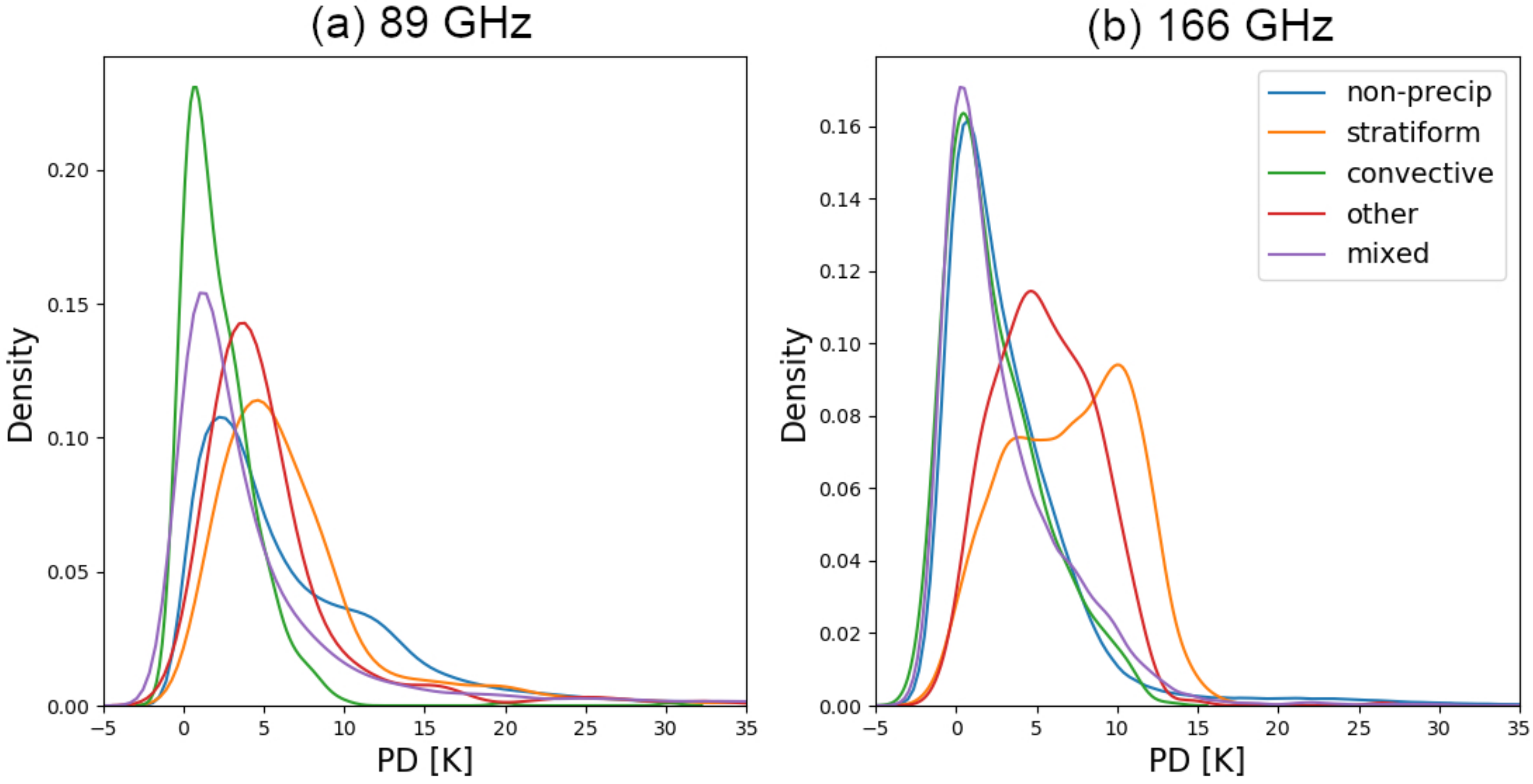
2.2.1. Polarization Differences

The main motivation behind creating hand-engineered features was to try to manually construct associations between variables which may prove to be useful in training the machine learning model. Polarization difference, or PD, was the most important hand-engineered feature for this training exercise. PD was defined as

$$PD=T{c}_V-T{c}_H{|}_{channelfrequency}$$

where $T{c}_V$ ($T{c}_H$) is the Level-1CR brightness temperature observed at vertically (horizontally) polarized channel. For GMI, there were a total of 5 channel pairs that had PDs, which were at 10.65, 18.7, 36.5, 89 and 166.5 GHz. An example of the PD distribution collected from a random day is given in Figure 2 for 89 and 166 GHz, where we see considerable differences between the distributions for different precipitation types. The disparity is especially pronounced between the $P{D}_{166\mathrm{GHz}}$ distributions under stratiform (blue) and convective (orange) scenarios. Ref. [28] previously found that large PD values at these two channels with medium cold $Tc$ values were explained by scattering from a layer composed of large horizontally oriented snow, which could only happen in the stratiform regime. Ref. [29] further identified PD’s positive association with stratiform precipitation occurrence as well as precipitation strength. Ref. [8] in the TRMM (Tropical Rainfall Measurement Mission; the predecessor of the GPM mission) era explored the use of 85 GHz PD for detecting stratiform rain from TRMM’s microwave imager (TMI; the predecessor of GMI) observations. As is shown in Section 3.3, $P{D}_{89\mathrm{GHz}}$ and $P{D}_{166\mathrm{GHz}}$ are proved again from an ML/AI perspective to be substantial factors in accurate precipitation type prediction.

2.2.2. Surface Emissivity

Surface Emissivity is a notoriously known to “contaminate” precipitation retrievals for PMW sensors as MW can penetrate through a top layer of land surfaces. It is particularly challenging to retrieve precipitation over snow-covered surfaces or certain desert surfaces because the signals they emit often exhibit similar features to precipitation [30]. Even for ocean surface where emissivity is relatively well understood, physics-based emissivity models often require a variety of inputs (e.g., ocean surface wind) that are usually not readily available or of poor quality (e.g., reanalysis data). For example, the GPM team currently uses an empirical surface emissivity model called TELSEM (Tool to Estimate Land-Surface Emissivities at Microwave frequencies) [31] for their precipitation product. This model uses a clustering approach to identify self-similar adjacent pixels on spatial and temporal grids from Special Sensor Microwave/Imager (SSM/I) observations to empirically retrieve surface emissivity from 19 to 89 GHz. For GMI, this means 10, 166, and 183 GHz emissivities are extrapolated; further, the spatial and temporal resolution is too coarse for GPM’s precipitation retrieval.

A recent work by [27] applied an optimal estimation (OE) approach to retrieve clear-sky emissivity from GMI’s clear-sky $Tc$s. The clear-sky flag was jointly determined by GMI, DPR, and MERRA-2 data. This emissivity database provides pixel-by-pixel land surface (including snow-covered and sea-ice-covered surfaces) emissivity retrievals at every GMI channel, and are hence easily adaptive features in our study. For precipitation- and/or ice-cloud-affected pixels, a larger ${\chi }^2$ value is produced that indicates a larger error in the emissivity retrieval. Liquid cloud also brings a negative impact on the emissivity retrieval error, so MERRA-2’s cloud liquid water path (CLWP) was also included in this product for users to screen out potential liquid-cloud-impacted scenes. Note that $CLWP$ was included as one of the 37 features as shown in Table 1, which should work as a liquid-cloud screening flag within the machine learning process.

One could argue that this emissivity database is a repetitive use of $Tc$ information and hence should not have been included in the features. Our rationale to include emissivity was as follows. Firstly, ${\chi }^2$ values were not included in the input features, so we were not repetitively using any existing precipitation or cloudy-sky flag information that was otherwise indicated by large ${\chi }^2$ values. Secondly, surface-induced PD signals are often hard to differentiate from cloud-induced PD signals, especially for low-frequency channels. Emissivity data over clear-sky pixels could help differentiate them. We elaborate more in Section 3.2 and Section 3.3 about the reasons why emissivities are among the top factors in determining a precipitation flag. Furthermore, a sensitivity experiment was carried out in Section 3.2 to remove emissivity as the input feature. As is shown in Section 3.2, removing emissivity had some marginal benefit for simple ML models, elevating the accuracy rate of “other” type but decreasing the accuracy of “convective” as a trade-off. For a more sophisticated model such as CNN, the impact is rather trivial.

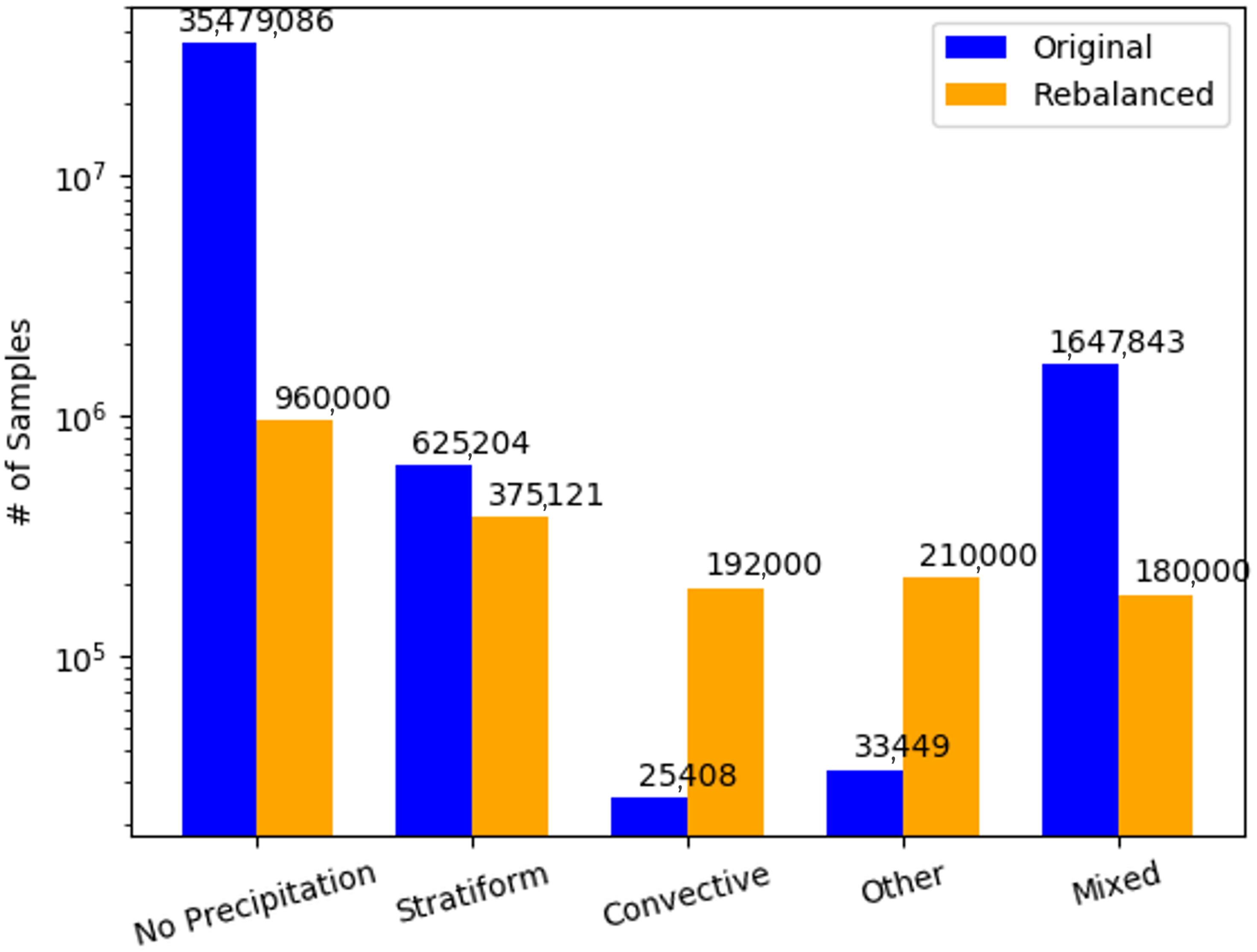
2.2.3. Sample Balancing

A challenge we had in this work was that some classes (i.e., no precipitation and mixed) had a notably higher number of data samples than other classes. The total number of samples under each precipitation type is shown in Figure 3 as blue bars (note that the vertical axis is in a log-scale to amplify the small sample size for “convective” and “other” types). This class imbalance could significantly compromise the process of learning because the model tended to focus on the prevalent class and to ignore the small classes with much less data samples. The scarcity of data from small classes resulted in poor estimates of the model’s accuracy of those classes.

To address the class imbalance problem, we used the random majority undersampling method [32] to reduce the class size by randomly removing data samples from the big classes (i.e., no precipitation and mixed). In addition, we used a smoothed bootstrap-resampling-based technique [33] to rebalance the class distribution for this imbalanced dataset. Essentially, we drew from the training dataset an example from each small class (i.e., “convective” and “other”) to generate a new example in its neighborhood, and retrained the models until the recall of the small class was maximized. The rebalanced sample size is shown as orange bars in Figure 3. Note that this rebalancing process was tuned to holistically maximize the accurate prediction rate for all 5 classes for the CNN model, while it was not necessarily the best choice for other simple ML models.

2.3. Machine Learning Models

For this project, we trained and evaluated 6 different machine learning models, which were support vector machine (SVM), logisitic regression (LR), random forest (RF), gradient boosting (GB), neural network (NN) and convolutional neural network (CNN). The former 5 models were trained, tuned, and evaluated using the Python scikit-learn package, while the CNN was constructed using the Python tensorflow package. The working mechanism/philosophy behind these models are briefly described below.

The support vector machine (SVM) model uses a subset of the training data, known as support vectors, and applies the combination of a kernel with a modified loss function to make predictions. The SVM was originally designed for binary classification but can be extended to multiclass classification as in our case via the one-versus-the-rest approach to maximize the margin from each to the remaining classes. The logistic regression model uses a logistic function to model the features and class variables by minimizing the sum of the squares of the residuals for each data sample in the training set. With a goal to reduce the variance of the prediction, the random forest, proposed in [34], trains different decision trees on different subsets of the training data, chosen randomly with replacement, and then computes the ensemble. It tries to decorrelate the base learners based on a randomly chosen subset of input variables. Such models often have very good predictive accuracy [35]. Moreover, we trained a multilayer perceptron model, a class of feedforward neural networks that use backpropagation for training in this work. We also trained an XGBoost model, a parallel gradient-boosted decision tree model that uses decision trees as weak prediction models in gradient boosting [36].

Convolutional neural networks (CNN) are specific types of neural networks that contain convolutional layers. They are based on the idea of transforming the input data with a set of differentiable operations with feature extraction, which allows them to learn meaningful representations of the data. In this work, we used a CNN composed of three types of layers: convolutional layer, max-pooling layer, and fully connected layer. The high-dimensional input data were fed to the convolutional layers and max-pooling layers. The last pooling layer replaced the output of the network at certain locations by deriving a summary statistic of the nearby outputs. This helped reduce the spatial size of the representation, which decreased the required amount of computation and weights. Then, the low-dimensional features were fed to the fully connected layers. Neurons in that layer had full connectivity with all neurons in the preceding and succeeding layers as seen in regular feed-forward neural networks.

3. Results

In this section, the statistical metrics from the testing datasets are first presented, and two models with the highest overall accuracy—GB and CNN—are selected for generating the final predictions. The final predictions from the full-swath GMI observations were evaluated from multiple perspectives, including their consistency with physical understandings, their view-angle dependencies, their performance on a single weather event, and their climatological distributions.

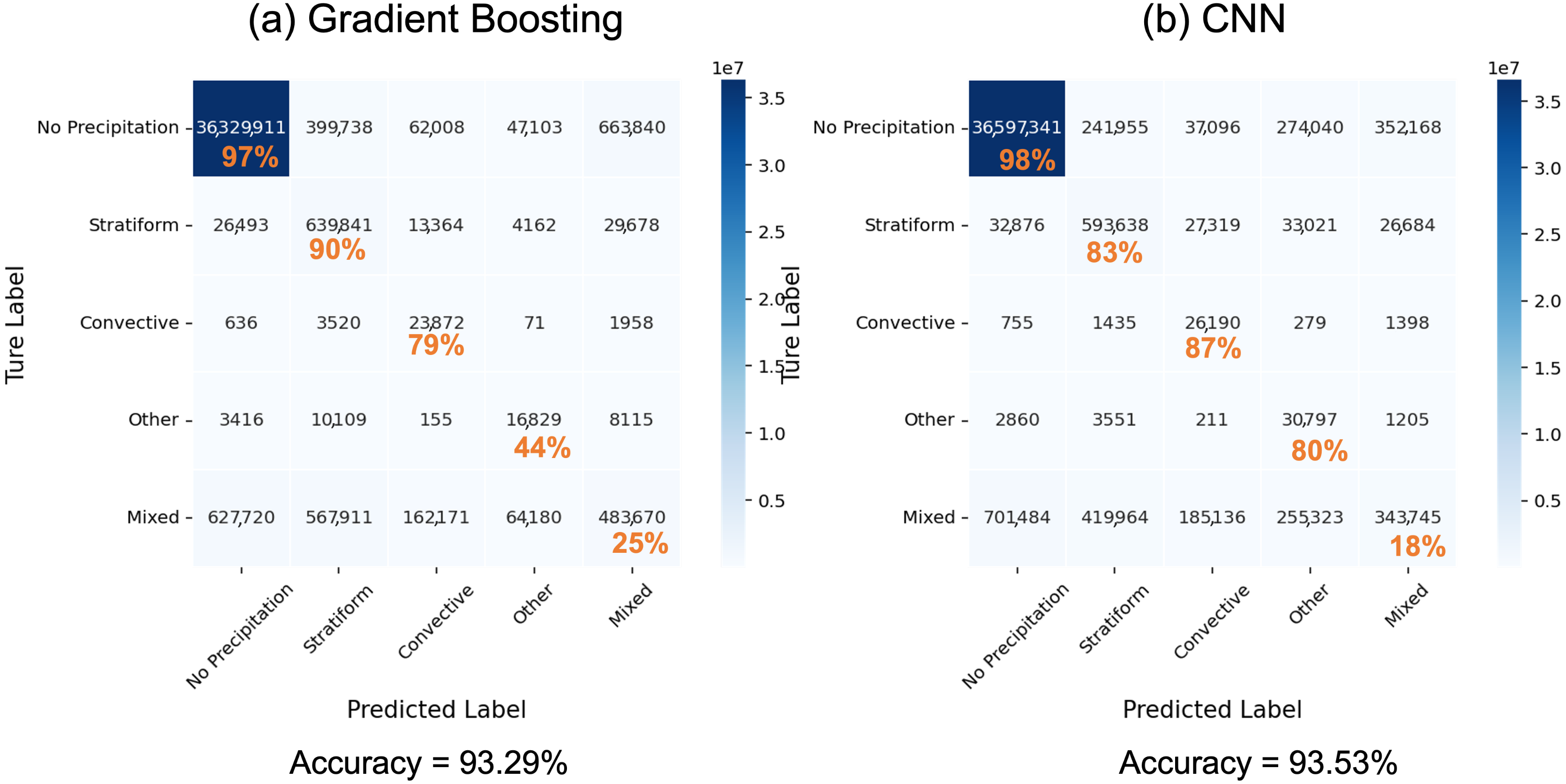
3.1. Prediction Accuracy

Two metrics were used for evaluating the model performance, the overall accuracy and the area under the ROC curve (AUC ROC). The overall accuracy was calculated by dividing the total number of correct predictions over all types by the total number of predictions (the number of data samples in the testing set). The AUC ROC score is a metrics to better evaluate the performance of a classifier, especially for highly imbalanced data [37]. The AUC ROC score for a classifier ranges from 0 to 1, where a score of 0.5 is given to a random classifier. From

Table 2. Comparison of prediction accuracy (%) and area under ROC curve (AUC ROC) from different ML/AI models tested. Three models that achieved the highest accuracies are highlighted in bold, and all results shown below are from these three models.

Classifier	Overall Accuracy (%)	AUC Score
Support Vector Machine (SVM)	91.15	N/A
Logistic Regression (LR)	76.07	0.8995
Gradient Boosting (GB)	93.31	0.9672
Random Forest (RF)	89.99	0.9594
Neural Network (NN)	93.56	0.9661
Convolutional Neural Network (CNN)	93.53	0.9678

, we can clearly see that the CNN produced overall the highest accuracy (93.53%). Four out of the five relatively simple ML models achieved similar accuracy at ∼90%, while the LR model performance was the lowest. As the GB model comes with explicit ranking of feature importance (Section 3.3) and it produced the second highest accuracy score, CNN and GB were selected for producing further statistics for comparison.

A further evaluation of the distribution of the accuracy (number of correct prediction out of total predictions) and misclassification rate in each precipitation category revealed that the accuracy rate was the highest for nonprecipitation scenes (top left cells in Figure 4). This is understandable from a physics point of view, as it is a relatively easier task to separate precipitating and nonprecipitating scenes, especially considering that more than half of the latter contained clear-sky pixels that were reflected by warmer $Tc$s at high-frequency channels. This fact is also expected from a computer science point of view, as ML model evaluations were carried out on sample-size weighted metrics in every layer, where nonprecipitation pixels still occupied the majority of samples even after rebalancing (Figure 3). We can also notice that although the deep learning model CNN produced only a slightly higher overall accuracy rate, it outperformed other simple ML models in the “other” precipitation category significantly.

Among the four types of precipitation, three monotype ones—stratiform, convective, and other—had comparable accuracies (80–87%) with the CNN. Figure 4 only showcases the results from the GB and CNN models, but the RF and NN models produced similar statistics (not shown). The robustness of the single-type precipitation accuracy using GMI-only data revealed that PMW like GMI could differentiate precipitation features at about 80–87% of the scenes, as long as the footprint was occupied by the same type of precipitation. Hence, it is important to have a small footprint size for PMW sensors, especially for convective precipitation scenes, as the area for convective precipitation is usually small and highly inhomogeneous. For the 16–20% scenes that were misclassified, features from them were likely ambiguous and a confident classification could not be made. For example, misclassified convective scenes were often assigned to the “stratiform” or “mixed” classes, which likely happened at the boundary of a convective cell and stratiform layer for weather systems such as mesoscale convective systems (MCSs) or winter frontal systems, while it was unlikely to be assigned to the “other” type, as the “other” precipitation is mainly associated with anvil clouds that are high in altitude and relatively thin in thickness, which hence usually produces less depression in the $Tc$ signal for the GMI channels [29].

The ML models can produce class probabilities in addition to class labels. In practice, we did not set a rigid threshold of probability to select the predicted class, but rather chose the one with the highest probability output, which is a normal fashion. In Figure 5, we reported the probability distribution for each class produced by the CNN model for the ones that were correctly (a) and wrongly predicted (b), respectively. Note that the negative value at the left tail of Figure 5b resulted from a plotting package artifact, while the true value was always between zero and one. One can see that apparently, the “mixed” type was the hardest to predict, as the CNN model was not very confident even when the prediction was correct by giving a probability value between 0.3 and 0.6. This was mainly because we assigned all GMI’s footprints with multiple DPR’s precipitation flags to this category, which was apparently not an optimal way for the classification. The confidence of the prediction in this category was also the lowest (purple line in Figure 5). We are currently exploring the optimal way of subgrouping under this “mixed” class. Other than this class, we can see the probability is a good measure of the confidence of the model performance for the other four categories.

Different from the probability, the uncertainty provides another measure of the quality of the prediction. Existing approaches based on Bayesian deep learning capture either aleatoric uncertainty or epistemic uncertainty for different tasks, e.g., in computer vision [38] and precipitation type classification [11,39]. These uncertainties are formalized as probability distributions of the model parameters and model outputs. As we did not employ a Bayesian model in this study, instead we employed a non-Bayesian approach. Ref. [40] showed that non-Bayesian solutions can produce good predictive uncertainty estimates on many tasks including classification task. We followed the notion of expected calibration error (ECE) in [40] as a measure of our model’s uncertainty. Specifically, ECE approximates the difference in expectation between a model’s confidence and accuracy. An ECE score runs between zero and one, with zero meaning the model is well-calibrated, as confidence closely approximates the expected accuracy. On the other hand, if ECE is close to one, the model is not highly confident about its prediction even if the model’s accuracy is better. One can see from the last column of

Table 3. Accuracy rate (%) with including emissivity and without emissivity in the training process for each precipitation class for GB, RF and CNN model from independent tests. The uncertainty score using the ECE method is listed in the last column, where we did not compute the score for “CNN-emis” model. See text in Section 3.1 for details of the uncertaincy calculation.

Classifier	Non-Precip (%)	Stratiform (%)	Convective (%)	Other (%)	Mixed (%)	Overall Accuracy (%)	ECE Score
GB + emis	97	90	79	44	25	93.29	0.557
GB − emis	97	87	83	76	20	92.78	0.554
RF + emis	92	85	74	43	45	89.99	0.547
RF − emis	94	86	73	66	36	91.29	0.553
CNN + emis	98	83	87	80	18	93.53	0.555
CNN − emis	97	86	86	80	15	92.68	–

that the ECE scores were close to one another among different models with adding or removing the emissivity inputs (see the following section for the sensitivity experiment). This means there was no significant difference regarding the model’s confidence. All three models listed in Table 3 had good performance in terms of both classification accuracy as well as ECE score.

To summarize, GMI-only prediction worked exceptionally well at distinguishing nonprecipitation and precipitation scenes (>97% accuracy rate for predicting a nonprecipitating scene). For precipitation scenes, GMI-only prediction worked for 80–87% of the cases when its footprint was occupied by one single type of precipitation if a CNN model was employed. It worked poorly when the footprint had large inhomogeneity or at the transition boundary between two major types. The latter point is demonstrated later by a weather event study in Section 4.

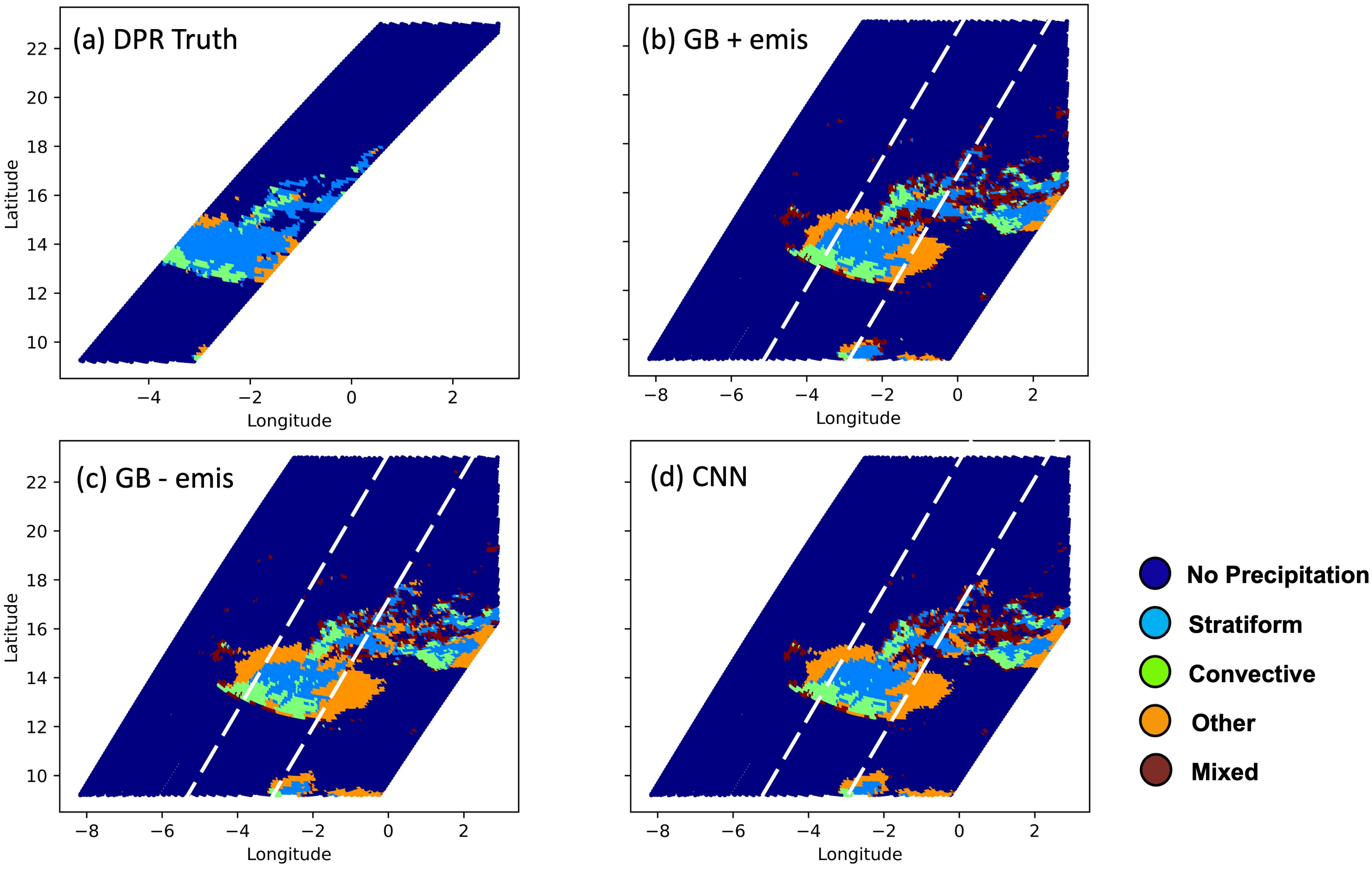
3.2. Sensitivity to Surface Emissivity

As emissivity was a new hand-engineered feature included in the training, it was necessary and beneficial to test how sensitive our trained models were with respect to these variables. The confusion matrices for the GB, RF and CNN models without emissivity are shown in Table 3. The overall accuracy change for every of the six ML models was less than 1% (only GB, RF and CNN results are shown). However, we can see from the statistics that excluding emissivity particularly further downgraded the capability of differentiating the signature for the “mixed” class category (numbers with underlines). For the CNN, the prediction accuracy for the other four monotype classes remained robust. Interestingly, however, for the other five simple ML models, prediction for the “other” type was significantly improved if the surface emissivity database was excluded for the training (bold numbers), while the other three monotypes remained robust.

Although it was a simple sensitivity test and we did not try to exclude emissivity at each channel one-by-one, the results were indicative of at least two important implications. Firstly, the fact that all six ML models remained robust in producing a high accuracy rate for the “nonprecipitation”, “stratiform” and “convective” classes indicates that these three monotypes were well separated in terms of the $T_c$ features in the multidimensional space. Such a separation is hard to model with radiative transfer models (RTMs) as hydrometeor scattering and absorption involve great variability and uncertainties; instead, even simple ML models can capture the feature separation easily. Second of all, the benefit of including surface emissivity in the training process is rather hard to determine. There is enough hint that including surface emissivity helps better identify the “mixed” class from the other types. However, the degradation and sensitivity of the “other” class from all five simple ML model to surface emissivity features suggests that the emissivity product itself might not be good enough to separate light precipitation against surface emissions. The deep learning CNN model was the only one among the six ML models that stayed robust against adding or removing emissivity in the training features.

3.3. Rank of Importance and Corresponding Physics Mechanisms

As described in Section 2.2, one of the most important novelties of this work is to include the PDs and retrieved surface emissivity for the training and prediction, both of which come with a solid radiative transfer theoretical basis. In this section, we demonstrate from the ML point of view how its results are consistent with the physical basis. This is a critical step to build-up physics-consistent retrieval algorithms using an ML/AI approach in the future.

For simple ML models such as GB and RF, the rank of the feature importance is provided together with the trained models. Feature importance refers to a class of techniques to assign a score to each input feature that indicates the marginal importance of each feature when a prediction is made. An RF model is essentially composed of a set of decision trees. For each decision tree, it is made from a set of internal nodes and leaves. The nodes determine how to divide the dataset into two different branches. The internal nodes are the most important features, and the ranking of the feature importance helps elucidate the important factors in the decision (or voting) process. The GB model employs a similar decision tree process, except it tries to minimize the cost function in each layer, rather than voting. This feature is not present in NN or CNN models. Here, only the top 15 most important features are listed in

Table 4. First 15 most important features listed for the GB and RF models with (+ emis) and without (− emis) emissivity in the training process. High-frequency channels $T_c$s are highlighted by bold letters, and $PD$s are further underlined.

Feature Importance Rank	GB + emis	RF + emis	GB − emis	RF − emis
1	$Emi{s}_{166H}$	$Emi{s}_{10V}$	CLWP	TWV
2	$Emi{s}_{10V}$	$Emi{s}_{10H}$	$\mathit{T}{\mathit{c}}_{\mathbf{166}\mathit{H}}$	$T_s$
3	CLWP	$Emi{s}_{166H}$	$\mathit{T}{\mathit{c}}_{\mathbf{166}\mathit{V}}$	$\mathit{T}{\mathit{c}}_{\mathbf{89}\mathit{V}}$
4	$Emi{s}_{10H}$	$\mathit{P}{\mathit{D}}_{\mathbf{89}}$	$T{c}_{36V}$	$\mathit{T}{\mathit{c}}_{\mathbf{183}/\mathbf{7}}$
5	$\mathit{T}{\mathit{c}}_{\mathbf{166}\mathit{H}}$	$\mathit{T}{\mathit{c}}_{\mathbf{89}\mathit{V}}$	$\mathit{T}{\mathit{c}}_{\mathbf{89}\mathit{V}}$	CLWP
6	$Emi{s}_{89H}$	CLWP	TWV	$\mathit{P}{\mathit{D}}_{\mathbf{89}}$
7	TWV	$Emi{s}_{89V}$	$\mathit{T}{\mathit{c}}_{\mathbf{183}/\mathbf{7}}$	$\mathit{T}{\mathit{c}}_{\mathbf{166}\mathit{H}}$
8	$\mathit{P}{\mathit{D}}_{\mathbf{89}}$	TWV	$\mathit{P}{\mathit{D}}_{\mathbf{89}}$	$\mathit{T}{\mathit{c}}_{\mathbf{166}\mathit{V}}$
9	$\mathit{T}{\mathit{c}}_{\mathbf{89}\mathit{V}}$	Ts	$\mathit{T}{\mathit{c}}_{\mathbf{183}/\mathbf{3}}$	$\mathit{T}{\mathit{c}}_{\mathbf{183}/\mathbf{3}}$
10	$\mathit{T}{\mathit{c}}_{\mathbf{166}\mathit{V}}$	$\mathit{T}{\mathit{c}}_{\mathbf{183}/\mathbf{7}}$	$T_s$	$\mathit{T}{\mathit{c}}_{\mathbf{89}\mathit{H}}$
11	$Emi{s}_{89H}$	$Emi{s}_{166V}$	$\mathit{P}{\mathit{D}}_{\mathbf{166}}$	$\mathit{P}{\mathit{D}}_{\mathbf{166}}$
12	$T_s$	$Emi{s}_{183/7}$	$\mathit{T}{\mathit{c}}_{\mathbf{89}\mathit{H}}$	$T{c}_{36V}$
13	$Emi{s}_{36V}$	$Emi{s}_{183/3}$	$T{c}_{10V}$	$T{c}_{24}$
14	$\mathit{P}{\mathit{D}}_{\mathbf{166}}$	$\mathit{P}{\mathit{D}}_{\mathbf{166}}$	$T{c}_{36H}$	$T{c}_{10V}$
15	$\mathit{T}{\mathit{c}}_{\mathbf{166}\mathit{H}}$	$\mathit{T}{\mathit{c}}_{\mathbf{166}\mathit{H}}$	$T{c}_{24}$	$T{c}_{36H}$

for the GB and RF models, with emissivity included in the training (+ emis) and without (− emis).

The first difference between “+ emis” and “− emis” experiments we can observe is the dominance of surface emissivities at 10, 89, and 166 GHz in the rank of importance if emissivity is included. In the meantime, $T_c$ values at 89 and 166 GHz also play some of the most dominant roles across the board. This indicates that there is a redundancy of input information at least for 89 and 166 GHz for surface emissivity characteristics. The original $T_c$ observations at these two channels contain enough distinctive surface emission and cloud scattering/emission signatures that can help us separate the five precipitation classes. When emissivity is removed from the input features, $T_c$ at the 183/3 and 183/7 GHz channels show up among the top ones. The high-frequency channels (>85 GHz) are much more sensitive to cloud ice and snow scattering rather than rain/liquid emission [41]. In contrast, classical PMW rainfall or liquid water path (LWP) retrieval channels (18–36 GHz; [42,43]) are not highly ranked in any of these models. All these findings strongly suggest that the precipitation type is more closely related to the cloud regime (frozen or liquid) above rather than surface precipitation characteristics, which is consistent with the definition of stratiform and convective for DPR’s retrievals. A stratiform pixel is identified in DPR’s profiles by the melting layer at ∼0 ${}^{\circ }$C, which reflects in changes at high-frequency MW channels and also in PDs [29]. Such a consistency suggests that an ML/AI technique can learn radiative transfer physics internally if the information is embedded in the training parameters, and a feature importance matrix such as that in Table 1 can be used to evaluate the consistency and may be used for channel optimization for future instrument designs.

The second commonality we can easily observe is that $PD$ at 89 and 166 GHz are ranked highly on the list for all four experiments, especially when surface emissivities are removed from the training. Furthermore, $P{D}_{89\mathrm{GHz}}$ ranks higher than $P{D}_{166\mathrm{GHz}}$ across the board. The frequency band 85–89 GHz is a band that is sensitive to both liquid-water emission and ice scattering. This complicated nonlinear feature makes it particularly challenging to simulate cloudy-sky $Tc$ signal at this band for RTMs. However, the ML models successfully identified the connection between the 89 GHz $PD$ and precipitation type, which is consistent with the previous findings in [8,29], where they identified the association between snow aggregates and the 85–89 GHz $PD$ in the stratiform layer using radiative transfer theories.

To summarize, the fact that $T_c$s at 89, 183/7, and 166 GHz are the top three direct radiance observations when determining the precipitation type suggests that precipitation type is tightly correlated with the middle troposphere snow amount and distribution, while the high ranks of $PD$s at 89 and 166 GHz indicate that snow microphysics details are closely related to precipitation type as well. It should be noted that these two variables are also useful to differentiate surface and cloud/precipitation when $T_c$ is relatively warm [29]. Interestingly, the liquid cloud water amount (CLWP) from the auxiliary MERRA-2 reanalysis data ranked among the top factors from all experiments, which fits into the common sense, as the liquid cloud layer is closer in vertical distance to the surface precipitation. The importance of the total water vapor (TWV) and surface temperature (Ts) were also learned by the ML models to differentiate clear-sky and cloudy-sky. Surface emissivities at 89, 166 and 10 GHz, when included, played a major role in determining a prediction. However, as the overall prediction accuracy barely dropped or even increased for certain types (Table 3) when the emissivity was excluded, it is temporarily concluded here that there is some redundant information between raw $T_c$ observations and surface emissivity at these channels. However, further thorough investigations are needed, for example, to understand whether including emissivity could help improve the “mixed” class prediction, as suggested in Table 3.

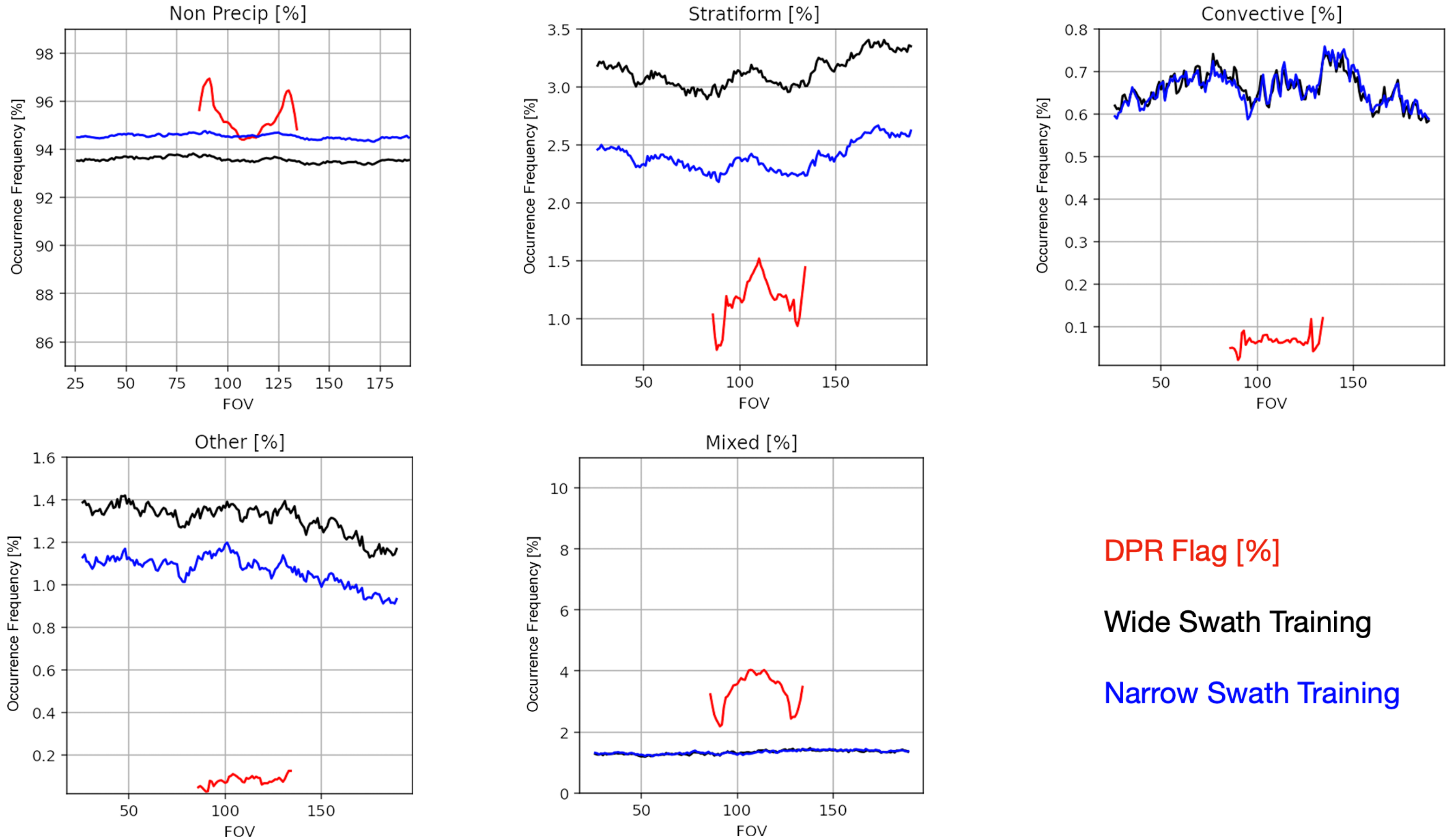
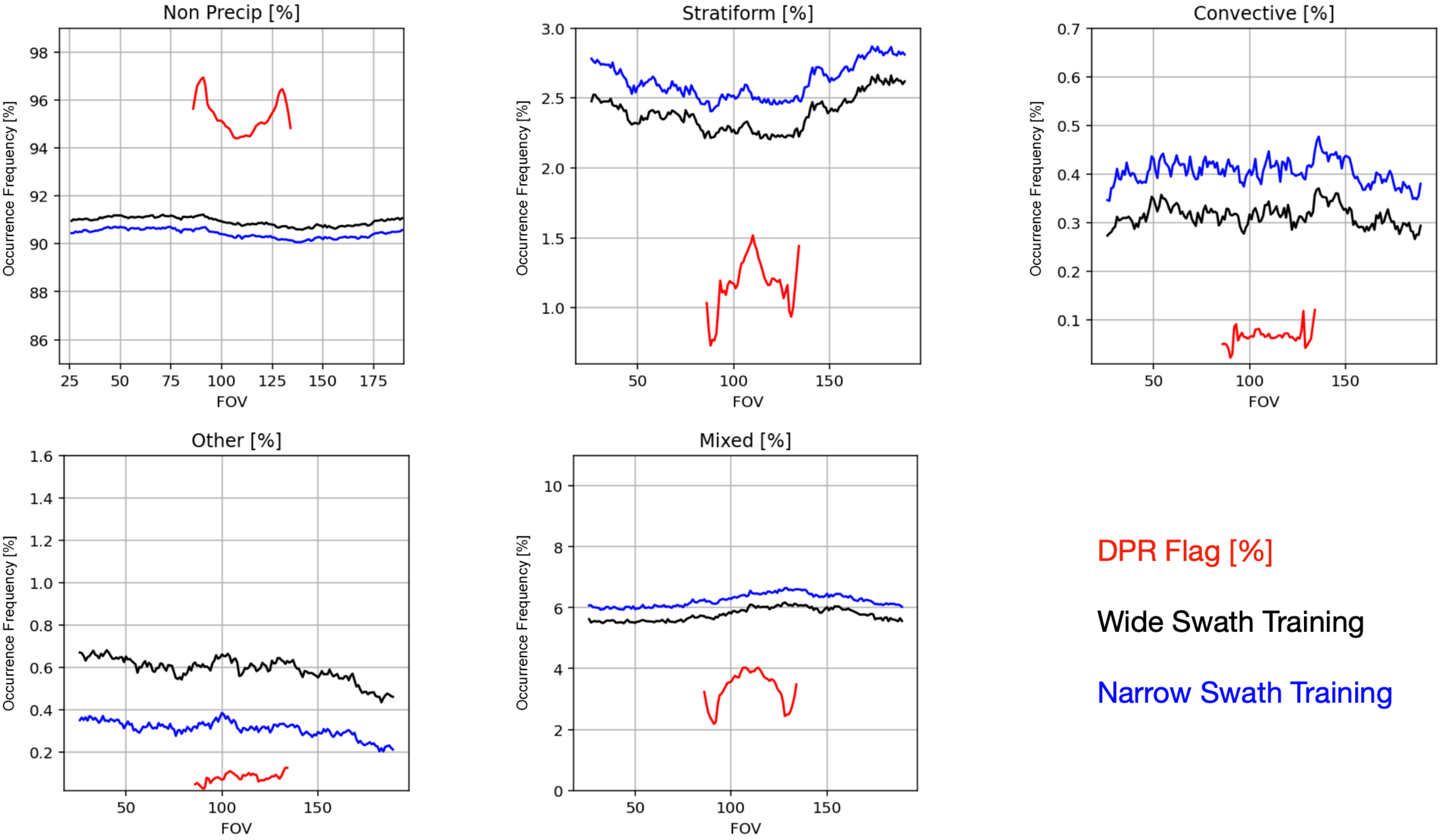
3.4. View-Angle Dependency

The DPR conducts cross-track scan consisting of 49 incidence angles in the range from $-{17}^{\circ }$ to ${17}^{\circ }$ relative to nadir for achieving a three-dimensional precipitation measurement. However, the measurements from off-nadir incidence angles are subject to contamination of surface clutter, leading to the DPR’s blind zone in which precipitation measurements are unavailable near the surface [25]. The degree of impact of surface clutter on the DPR’s precipitation measurements near the surface depends on the incidence angle and surface roughness. In general, the near-surface range contaminated by surface clutter increases with an increase of the off-nadir incidence angles. This caveat poses a practical problem in detecting shallow rain and classifying precipitation type when the bright-band/melting layer is close to the surface [44]. Moreover, the precipitation retrieval cannot be made without assumption in the blind zone. As the influence of surface clutter on the DPR’s measurements depends on the incidence angle, it is expected that some of the DPR product might exhibit angle dependence to various degrees. Therefore, it is intriguing and beneficial to study the view-angle dependency of the GMI-only retrieval product to understand whether the view-angle dependent artifact in the DPR product is propagated toward GMI or not.

The GMI’s and DPR’s precipitation occurring frequency (OF) as a function of the view-angle are shown for each precipitation type in Figure 6 for the GB model and Figure 7 for the CNN model outputs. “Wide-swath training” (Black lines in Figure 6) corresponds to the entire NS swath, while “narrow-swath training” (blue lines in Figure 6) corresponds to only the near-nadir 20 Ku-DPR’s footprints. The latter was a sensitivity experiment to test whether mitigating the DPR’s precipitation flag artifact at off-nadir angles would or would not affect the training results.

Evidently, DPR’s off-nadir artifact is clearly seen for the nonprecipitating, stratiform, and mixed classes. These are the three most frequently occurring types globally. Luckily, GMI did not learn this view-angle-dependent artifact because view-angle was not an input feature for the training. Rather, for this 1D retrieval, GMI treated each DPR view independently and hence did not propagate this error to larger oblique view angles. As a sensitivity study, we limited the training “truth” to only the near-nadir 20 DPR footprints (10 on each side), but the prediction results barely changed in terms of the view-angle dependency, although there was a hint that the narrow-swath training tended to result in predicting more stratiform and convective precipitations, while the “other” class tended to be less predicted (Figure 6).

Comparing the results generated from GB versus the CNN, the CNN’s prediction for nonprecipitation scenes were closer to that of the DPR. However, if we closely inspect the breakout from Figure 6 and Figure 7, there is not much difference between them for stratiform, convective, and other precipitation types, except the CNN model predicts 50% more convective and 60% more other types of precipitation compared to GB and RF (not shown) results. All three models overestimated the monotype precipitations, which may likely not indicate a bias, but rather a sensitivity of GMI to light precipitation that DPR is not sensitive to. This was also found previously in [22,27]. A future sensitivity study using the MS as the “truth” could help better elucidate this point and quantify the difference. The GB results overpredicted the occurrence chance for the “mixed” class while the CNN showed the opposite result. Since the accuracy rate for the “mixed” class was low for all the models, it was not very meaningful to compare their prediction.

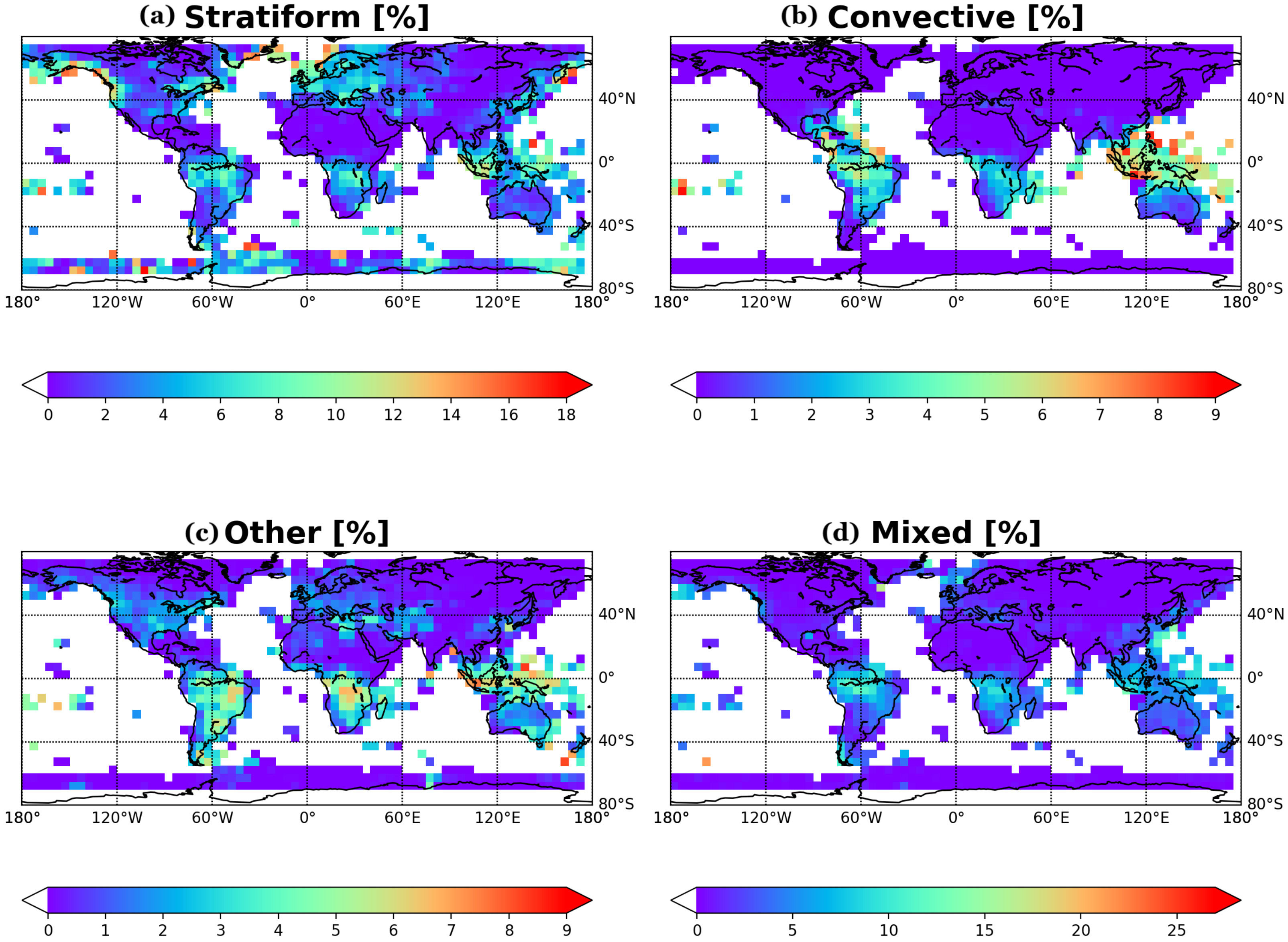
4. Application of GMI-Only Prediction on Weather and Climate Studies

The spatial and temporal distribution of each precipitation type is not only critical for making good weather forecast and potentially useful for enhancing weather-related warning products, its occurring frequency (OF) is also a straightforward matrix that can be used for comparing with GCM outputs, as GCM produces convective, stratiform, and anvil precipitation separately in each grid box [3]. In this section, we showcase the power of using GMI-only precipitation type classification for weather and climate research.

A squall line case passed by Mali, Africa on 6 June 2017, which was captured by the DPR and GMI. On the Ku-DPR’s retrieval shown in Figure 8a, the major squall line body, including the front line of convective cells (green), the large stratiform tail (blue), and the periphery anvil precipitation (orange), are well captured. We can further see another line of convection forming at its tail that seems to propagate northwestward, and the tip of another smaller squall line at the bottom right corner of the DPR swath. The full-swath (850 km) GMI-only prediction using the GB and CNN models are shown in Figure 8b–d, respectively, while the DPR swaths are bounded by the white dashed lines to ease a visual comparison. One can clearly see the overall structure agrees very well along the overlapped swaths, but the GMI also captures the long and complicated “goldfish tail” structure, and the other squall line system in the lower bottom corner. Further, the GMI prediction captures the anvil-head-associated precipitation signal ahead of the convection line (other, orange) which the DPR missed probably due to its low reflectivity. This anvil-head precipitation was previously identified in [29] from an ensemble collection of squall line cases that the GMI captured but the DPR missed.

Subtle differences were identified among the three model outputs. Notably the GB-emis model (Figure 8c) produced some convective flags in the middle of the vast area of stratiform trailing layers which the DPR did not observe, nor did the CNN and GB+emis models predict. A further inspection of the DPR’s vertical structure along the nadir path of the DPR swath (Figure 9) suggests that the CNN and GB+emis model predictions were of more fidelity for this case. As shown in Figure 9, the bright-band signature corresponding to the stratiform precipitation is evident in scan # 2305–2330 (black box). Yet, the enhancement of the Ku-DPR reflectivity at ∼scan #2305 indicates larger hydrometeor sizes or a stronger melting signature, which the GMI may likely capture and the GB-emis model learned. Besides this disparity, the GB-emis model predicted the least “stratiform” area and the most “other” precipitation area in the periphery of the main storm, while the GB+emis and CNN model results compared better with the DPR “truth”. We can find from this case study that including emissivity helped improve the overall quality for mesoscale weather systems. This is just a speculation, and extensive case studies will have to be carried out before any conclusion can be drawn. Furthermore, all three models predicted a lot of “mixed” pixels along the long gold fish tail, which apparently preferred to occur at the boundary of stratiform and nonprecipitating pixels. This fact supported our speculation that the mixed class tended to be overpredicted in a GMI-only product mainly because of the coarser resolution of the GMI’s footprint. Overall, we can conclude again from this case study that the three monotypes (nonprecipitating, stratiform, and convective) stayed robust against which ML model to choose. There were subtle differences, but the underlying physics played the dominant role. For the “other” and “mixed” classes, as the DPR has difficulties to sense light precipitation, and our “mixed” class was not well defined, we did not expect our model to produce very good results; nevertheless, they were still useful especially for the “other” type using the CNN model.

The global distribution of OF for each precipitation type is shown in Figure 10 for the CNN prediction for the boreal winter of 2017 (January, February, and December). The geographic distribution of stratiform and convective precipitation OFs agrees very well with previously reported features using TRMM-PR and GPM-DPR in the tropics and sub-tropics ([1,45]; and Figure 11 below). As expected, stratiform precipitations are found over tropical convection active centers as well as along the boreal winter storm tracks, while convective precipitations are found to frequently occur in the tropical convection active centers (i.e., Amazonia, Central Africa and West Pacific/Maritime continents). Because of the conical-scan geometry, the GMI covers a little bit more high-latitude areas than the DPR, and it is noticeable that stratiform precipitation occurs frequently over Southern Ocean above the sea-ice-covered area (i.e., where MERRA-2 has a land surface temperature retrieval), especially near the Antarctica Penninsula and McMurdo station where persistent mixed-phase cloud and associated pockets of ice precipitation have been reported in several ground measurement works [46,47]. Although all passive sensors have issues at snow/ice covered surfaces, the good comparison between the DPR and GMI-only prediction over the Antarctic sea ice suggests that high-frequency polarized passive MW measurements may provide some capability at distinguishing surface ice from frozen hydrometeors aloft in the air.

Here, we found “other” precipitation also occurred quite often in the similar regions where stratiform and convective precipitations prefer to happen, but the former generally covered a broader area. “Other” precipitation occurred as frequently as convective and stratiform precipitations in most of the tropical land areas. There were significant regional differences in terms of their relative importance. For example, in maritime continents—West Pacific area, convective precipitation occurred as frequently as stratiform precipitation, while that was not the case at other tropical convection active areas. We can also find convective precipitation rarely occurred over the winter storm tracks. As an extension of the North America storm track, the Middle East winter-time precipitation nearly all came from stratiform and “other” type of precipitations. Previous research had never reported a distribution of “other” type of precipitation to the authors’ best knowledge, probably because it is thought to happen less frequently due to the fact that precipitation radars such as TRMM-PR and GPM-DPR often miss to detect them. As also demonstrated in Figure 11, the “other” type saw by the DPR was in general one order of magnitude smaller than what GMI saw. At this point it is still too early to associate “other” class to anvil precipitation, but it is strongly indicated as such, and we will inspect collocated CloudSat radar echos to further study this type of precipitation. Part of the “other” type could also be associated with shallow convection or light precipitation that the DPR is not sensitive to.

Another merit of this GMI-only precipitation flag product is that one can construct and study the diurnal cycle of precipitation type. The diurnal cycle of precipitation is a well-known challenge for climate models to represent (e.g., [2]). In the tropics and mid-latitude summer, convection is thought to be responsible for initiating the precipitation processes. However, the time scale it takes for the decaying/dissipation processes determines the spread area and intensity of stratiform precipitation. Hence, it is necessary and a great benefit this product can bring to the precipitation community to separate out the diurnal cycle of different precipitation processes. In the winter hemisphere, it is stratiform precipitation process that dominates the surface precipitation variation, and hence it is more meaningful to single out this type of precipitation and study it.

GPM flies on a large inclination angle (${65}^{\circ }$) to cover high latitudes, hence it takes more than 3 months to sample the entire diurnal cycle at different latitudes. For this consideration, we combined June, July, and August (JJA) of 2016 and 2017 GMI-only predictions together to generate the diurnal cycle contours for different latitude bands shown in Figure 12 for DJF and Figure 13 for JJA. In the tropics, as well observed and reported before, convection peaks in the late afternoon, but we can still see the peak time tends to drift toward a later time moving away from the equator. The peak and trough of the diurnal cycle of the “other” class follows closely with that of the deep convection with a lag of about 2–3 h. This strongly indicates that the “other” class is associated with anvil precipitation which is subject to the development and dissipation of the convective core. However, the decay of stratiform precipitation takes a significantly longer time and has subtle latitudinal variations that do not follow closely with that of the deep convection.

Interestingly enough, the stratiform precipitation over the Southern Ocean wintertime (Figure 13) exhibits a distinctive diurnal cycle with peak occurrence at local night to early morning and a quiet period of precipitation in local afternoon. This is consistent with Macquarie Island’s ground rain gauge observations [48]. However, the summertime (Figure 12) diurnal cycle disagrees with ground measurements in the same paper. Boreal winter storm tracks also exhibit a weak but interesting diurnal cycle. These discrepancies and new features warrant further investigations.

5. Conclusions

This work developed a machine learning/artificial intelligence (ML/AI) approach to retrieval precipitation types from passive microwave (PMW) radiometers/imagers. This approach was applied to collocated GPM-GMI and GPM-DPR data, where the latter was used as the “truth” for training, validation, and independent testing. In principle, this approach can be easily extended to other spaceborne PMW instruments as the DPR overpasses frequently with polar orbiting satellites.

Different ML models were trained to classify five precipitation types and to make predictions simultaneously. The five types were (0) nonprecipitating; (1) stratiform; (2) convective; (3) other; and (4) mixed. The last class was created when the GMI footprint was filled with multiple DPR’s footprints that did not share the same precipitation type as the first four. A total of six ML models were tested, and only the logistic regression model failed to make a good prediction. Gradient boosting (GB) and the convolutional neural network (CNN) produced overall the highest accuracy at 96.7%. Although the overall accuracy was sample-size-weighted (i.e., total correct samples divided by total samples), the GMI-only CNN prediction was correct 80–87% of the time when it was precipitating, and the scene was filled with a single type of precipitation. Challenges were identified for the mixed class as the radiance signal was rather a mixture of different precipitation categories.

Different from previous ML/AI explorations on a similar topic (e.g., [17]), this work strove to separate nonprecipitation (>95% of the time) and precipitation scenes simultaneously by predicting the precipitation types, so the training dataset was extremely unbalanced. A data augmentation was subsequently introduced to subset the nonprecipitation scenes and bootstrap from the “convective” and “other” sample pools. This data augmentation technique is particularly useful for precipitation-related science as data imbalance frequently occurs in this field.

Other than using all 13 GMI channel observations and some ancillary features from the MERRA-2 reanalysis, the most important novelty of this work was to include hand-engineered features—polarization difference (PD), and emissivity retrieval products. Including these attributes turned out to be extremely useful, as PDs and emissivities at high-frequency (>89 GHz) channels were ranked among the top ones for making a precipitation type prediction. Simple ML models were sensitive to the emissivity by showing a trade-off of accuracy rate between the “other” and “mixed” classes. The deep learning CNN model remained robust with or without the surface emissivity included in the training features. We demonstrated in this paper how an ML model could learn the radiative transfer physics internally and reach microphysics- and emissivity-consistent results. This finding adds fidelity to use the ML/AI approach for developing retrieval algorithms.

While many of the current spaceborne PMW instruments have high-frequency channels, they barely hold the dual-polarized channel pairs nor have a pixel-by-pixel emissivity retrieval product readily available. This poses challenges for achieving high accuracy in predicting precipitation types from other PMW instruments using this approach, and it will be a good exercise for future works. Other possible future working directions could include assessing light precipitation and “other” precipitation from GMI-only predictions against collocated CloudSat data to further understand the capability or limitations of the GMI’s precipitation retrieval.

Besides demonstrating the advantages of using the GMI’s precipitation type retrievals for weather and climate studies, we identified two particular merits that GMI’s precipitation type retrieval exhibited while the DPR did not. Firstly, the DPR’s view-angle dependent artifact does not propagate into GMI’s oblique view angles. Combined with the fact that microphysical signals embedded in the PD observation are less complicated in a fixed view-angle conical scanner, this finding implies that conical scanning is a better design for future PMW instruments compared to cross-track scan, if mission budget is not factored in. Secondly, the GMI’s precipitation type retrieval captures more light precipitation scenes than that of the DPR, especially for the “other” type. Both findings suggest that ML/AI can not only learn from the “truth”, but it also has the capability to unearth embedded information in the training features that is highly intertwined and nonlinear that RTM simulations cannot reveal.

Admittedly the current work is far from a complete study. The quality of the DPR’s precipitation flag retrieval has not been widely assessed globally, so we do not have a good knowledge of the quality of the “truth” dataset. Consequently, the probability prediction (e.g., Figure 5) apparently does not include the uncertainty of the “truth” dataset. The GMI-only product should also be assessed against ground observations globally, especially at known difficult places such as coastal, arid, mountainous, or snow/ice-covered surfaces. These remain to be potential areas for future investigation.

References

1. Yang, S.; Smith, E.A. Convective–Stratiform Precipitation Variability at Seasonal Scale from 8 Yr of TRMM Observations: Implications for Multiple Modes of Diurnal Variability. J. Clim. 2008, 21, 4087–4114. [Google Scholar] [CrossRef]
2. Bosilovich, M.G.; Akella, S.; Coy, L.; Cullather, R.; Draper, C.; Gelaro, R.; Kovach, R.; Liu, Q.; Molod, A.; Norris, P.; et al. MERRA-2: Initial Evaluation of the Climate. Available online: https://gmao.gsfc.nasa.gov/pubs/docs/Bosilovich803.pdf (accessed on 4 May 2022).
3. Yuan, W.; Yu, R.; Zhang, M.; Lin, W.; Li, J.; Fu, Y. Diurnal cycle of summer precipitation over subtropical East Asia in CAM5. J. Clim. 2013, 26, 3159–3172. [Google Scholar] [CrossRef]
4. Liao, L.; Meneghini, R. GPM DPR Retrievals: Algorithm, Evaluation, and Validation. Remote Sens. 2022, 14, 843. [Google Scholar] [CrossRef]
5. Seto, S.; Iguchi, T.; Meneghini, R.; Awaka, J.; Kubota, T.; Masaki, T.; Takahashi, N. The Precipitation Rate Retrieval Algorithms for the GPM Dual-frequency Precipitation Radar. J. Meteorol. Soc. Jpn. 2021, 99, 205–237. [Google Scholar] [CrossRef]
6. Petković, V.; Kummerow, C.D.; Randel, D.L.; Pierce, J.R.; Kodros, J.K. Improving the Quality of Heavy Precipitation Estimates from Satellite Passive Microwave Rainfall Retrievals. J. Hydrometeorol. 2018, 19, 69–85. [Google Scholar] [CrossRef]
7. Henderson, D.S.; Kummerow, C.D.; Marks, D.A.; Berg, W. A Regime-Based Evaluation of TRMM Oceanic Precipitation Biases. J. Atmos. Ocean. Technol. 2017, 34, 2613–2635. [Google Scholar] [CrossRef]
8. Olson, W.S.; Hong, Y.; Kummerow, C.D.; Turk, J. A Texture-Polarization Method for Estimating Convective–Stratiform Precipitation Area Coverage from Passive Microwave Radiometer Data. J. Appl. Meteorol. 2001, 40, 1577–1591. [Google Scholar] [CrossRef] [Green Version]
9. Islam, T.; Srivastava, P.K.; Dai, Q.; Gupta, M.; Jaafar, W. Stratiform/convective rain delineation for TRMM microwave imager. ScienceDirect 2015, 133, 25–35. [Google Scholar] [CrossRef]
10. Hong, Y.; Kummerow, C.D.; Olson, W.S. Separation of convective and stratiform precipitation using microwave brightness temperature. J. Appl. Meteorol. Clim. 1999, 38, 1195–1213. [Google Scholar] [CrossRef] [Green Version]
11. Orescanin, M.; Petković, V.; Powell, S.W.; Marsh, B.R.; Heslin, S.C. Bayesian deep learning for passive microwave precipitation type detection. IEEE Geosci. Remote Sens. Lett. 2021, 19, 1–5. [Google Scholar] [CrossRef]
12. Wang, C.; Platnick, S.; Meyer, K.; Zhang, Z.; Zhou, Y. A machine-learning-based cloud detection and thermodynamic-phase classification algorithm using passive spectral observations. Atmos. Meas. Tech. 2020, 13, 2257–2277. [Google Scholar] [CrossRef]
13. Robbins, D.; Poulsen, C.; Siems, S.; Proud, S. Improving discrimination between clouds and optically thick aerosol plumes in geostationary satellite data. Atmos. Meas. Tech. Discuss. 2022, 15, 3031–3051. [Google Scholar] [CrossRef]
14. Gong, J.; Wang, C.; Wu, D.L.; Barahona, D.; Tian, B.; Ding, L. A GCM-Oriented and Artificial Intelligence Based Passive Microwave Diurnal Ice/Snow Cloud Retrieval Product using CloudSat/CALIPSO as the Baseline. Atmos. Chem. Phys. 2022, 2021, A14B-07. [Google Scholar]
15. Upadhyaya, S.A.; Kirstetter, P.-E.; Kuligowski, R.J.; Gourley, J.J.; Grams, H.M. Classifying precipitation from GEOS satellite observations: Prognostic model. Q. J. R. Meteorol. Soc. 2021, 147, 3394–3409. [Google Scholar] [CrossRef]
16. Upadhyaya, S.A.; Kirstetter, P.-E.; Kuligowski, R.J.; Searls, M. Classifying precipitation from GEO satellite observations: Diagnostic model. Q. J. R. Meteorol. Soc. 2021, 147, 3318–3334. [Google Scholar] [CrossRef]
17. Petkovic, V.; Orescanin, M.; Kirstetter, P.; Kummerow, C.; Ferraro, R. Enhancing PMW Satellite Precipitation Estimation: Detecting Convective Class. J. Atmos. Ocean. Technol. 2019, 36, 2349–2363. [Google Scholar] [CrossRef]
18. Iguchi, T.; Seto, S.; Meneghini, R.; Yoshida, N.; Awaka, J.; Kubota, T. GPM/DPR Level-2 Algorithm Theoretical Basis Document, Version 06 Updates. 2018. Available online: https://gpm.nasa.gov/sites/default/files/2019-05/ATBD_DPR_201811_with_Appendix3b.pdf (accessed on 4 May 2022).
19. Awaka, J.; Iguchi, T.; Okamoto, K.T. Early results on rain type classification by the Tropical Rainfall Measuring Mission (TRMM) precipitation radar. In Proceedings of the 8th URSI Commission F Triennial Open Symposium, Aveiro, Portugal, 22–25 September 1998; pp. 143–146. [Google Scholar]
20. Awaka, J.; Iguchi, T.; Okamoto, K. TRMM PR standard algorithm 2A23 and its performance on bright band detection. J. Meteorol. Soc. 2009, 87, 31–52. [Google Scholar] [CrossRef] [Green Version]
21. GPM Intercalibration (X-CAL) Working Group. Algorithm Theoretical Basis Document (ATBD), NASA Global Precipitation Measurement (GPM) Level 1C Algorithms (Version 1.6). 2016. Available online: https://gpm.nasa.gov/sites/default/files/2020-05/L1C_ATBD_v1.6_V04_0.pdf (accessed on 4 May 2022).
22. Turk, F.J.; Ringerud, S.E.; Camplani, A.; Casella, D.; Chase, R.J.; Ebtehaj, A.; Gong, J.; Kulie, M.; Liu, G.; Milani, L.; et al. Applications of a CloudSat-TRMM and CloudSat-GPM Satellite Coincidence Dataset. Remote Sens. 2021, 87, 2264. [Google Scholar] [CrossRef]
23. Suzuki, K.; Kamamoto, R.; Nakagawa, K.; Nonaka, M.; Shinoda, T.; Ohigashi, T.; Minami, Y.; Kubo, M.; Kaneko, Y. Ground Validation of GPM DPR Precipitation Type Classification Algorithm by Precipitation Particle Measurements in Winter. SOLA 2019, 15, 94–98. [Google Scholar] [CrossRef]
24. Tan, J.; Petersen, W.A.; Kirchengast, G.; Goodrich, D.C.; Wolff, D.B. Evaluation of Global Precipitation Measurement Rainfall Estimates against Three Dense Gauge Networks. J. Hydrometeorol. 2018, 19, 517–532. [Google Scholar] [CrossRef]
25. Grecu, M.; Bolvin, D.; Heymsfield, G.M.; Lang, S.E.; Olson, W.S. Improved parameterization of precipitation fluxes in the GPM combined algorithm to mitigate ground clutter effects. In Proceedings of the AGU Fall Meeting, New Orleans, LA, USA, 13–17 December 2021; Available online: https://agu.confex.com/agu/fm21/meetingapp.cgi/Paper/953816 (accessed on 4 May 2022).
26. Grecu, M.; Olson, W.S.; Munchak, S.J.; Ringerud, S.; Liao, L.; Haddad, Z.; Kelley, B.L.; McLaughlin, S.F. The GPM Combined Algorithm. J. Atmos. Ocean. Technol. 2016, 33, 2225–2245. [Google Scholar] [CrossRef]
27. Munchak, S.J.; Ringerud, S.; Brucker, L.; You, Y.; de Gelis, I.; Prigent, C. An Active–Passive Microwave Land Surface Database From GPM. IEEE Trans. Geosci. Remote Sens. 2020, 58, 6224–6242. [Google Scholar] [CrossRef]
28. Gong, J.; Wu, D.L. Microphysical properties of frozen particles inferred from Global Precipitation Measurement (GPM) Microwave Imager (GMI) polarimetric measurements. Atmos. Chem. Phys. 2017, 17, 2741–2757. [Google Scholar] [CrossRef] [PubMed] [Green Version]
29. Gong, J.; Zeng, X.; Wu, D.L.; Munchak, S.J.; Li, X.; Kneifel, S.; Ori, D.; Liao, L.; Barahona, D. Linkage among ice crystal microphysics, mesoscale dynamics, and cloud and precipitation structures revealed by collocated microwave radiometer and multifrequency radar observations. Atmos. Chem. Phys. 2020, 20, 12633–12653. [Google Scholar] [CrossRef]
30. Prigent, C. Precipitation retrieval from space: An overview. C. R. Geosci. 2010, 342, 380–389. [Google Scholar] [CrossRef]
31. Aires, F.; Prigent, C.; Bernardo, F.; Jiménez, C.; Saunders, R.; Brunel, P. A tool to estimate land-surface emissivities at microwave frequencies (TELSEM) for use in numerical weather prediction. Q. J. R. Meteorol. Soc. 2011, 137, 690–699. [Google Scholar] [CrossRef] [Green Version]
32. Japkowicz, N.; Stephen, S. The class imbalance problem: A systematic study. Intell. Data Anal. 2002, 6, 429–449. [Google Scholar] [CrossRef]
33. Menardi, G.; Torelli, N. Training and assessing classification rules with imbalanced data. Data Min. Knowl. Discov. 2014, 28, 92–122. [Google Scholar] [CrossRef]
34. Breiman, L. Random forest. Mach. Learn. 2001, 24, 123–140. [Google Scholar] [CrossRef] [Green Version]
35. Caruana, R.; Niculescu-Mizil, A. An empirical comparison of supervised learning algorithms. In Proceedings of the 23rd International Conference on Machine Learning, Pittsburgh, PA, USA, 25–29 June 2006. [Google Scholar] [CrossRef] [Green Version]
36. Friedman, J.H. Greedy function approximation: A gradient boosting machine. Ann. Stat. 2001, 29, 1189–1232. [Google Scholar] [CrossRef]
37. Branco, P.; Torgo, L.; Ribeiro, R.P. A survey of predictive modeling on imbalanced domain. ACM Comput. Surv. 2016, 49, 1–50. [Google Scholar] [CrossRef]
38. Kendall, A.; Gal, Y. What uncertainties do we need in bayesian deep learning for computer vision? In Proceedings of the Advances in Neural Information Processing Systems, Long Beach, CA, USA, 4–9 December 2017.
39. Ortiz, P.; Orescanin, M.; Petković, V.; Powell, S.W.; Marsh, B. Decomposing Satellite-Based Classification Uncertainties in Large Earth Science Datasets. IEEE Trans. Geosci. Remote Sens. 2022, 60, 1–11. [Google Scholar] [CrossRef]
40. Guo, C.; Pleiss, G.; Sun, Y.; Weinberger, K.Q. On calibration of modern neural networks. In Proceedings of the International Conference on Machine Learning, Sydney, Australia, 6–11 August 2017; pp. 1321–1330. [Google Scholar]
41. Skofronick-Jackson, G.M.; Wang, J.R.; Heymsfield, G.M.; Hood, R.; Manning, W.; Meneghini, R.; Weinman, J.A. Combined Radiometer-Radar Microphysical Profile Estimations with Emphasis on High Frequency Brightness Temperature Observations. J. Appl. Meteorol. 2003, 42, 476–487. [Google Scholar] [CrossRef] [Green Version]
42. O’Dell, C.W.; Wentz, F.; Bennartz, R. Cloud Liquid Water Path from Satellite-Based Passive Microwave Observations: A New Climatology over the Global Ocean. J. Clim. 2008, 21, 1721–1739. [Google Scholar] [CrossRef]
43. Choi, Y.; Shin, D.-B.; Kim, J.; Joh, M. Passive Microwave Precipitation Retrieval Algorithm With A Priori Databases of Various Cloud Microphysics Schemes: Tropical Cyclone Applications. IEEE Trans. Geosci. Remote Sens. 2020, 58, 2366–2382. [Google Scholar] [CrossRef]
44. Awaka, J.; Le, M.; Brodzik, S.; Kubota, T.; Masaki, T.; Chandrasekar, V.; Iguchi, T. Improvements of rain type classification algorithms for a full scan mode of GPM Dual-frequency Precipitation Radar. J. Meteorol. Soc. Jpn. 2021, 99, 1253–1270. [Google Scholar] [CrossRef]
45. Gao, J.; Tang, G.; Hong, Y. Similarities and Improvements of GPM Dual-Frequency Precipitation Radar (DPR) upon TRMM Precipitation Radar (PR) in Global Precipitation Rate Estimation, Type Classification and Vertical Profiling. Remote Sens. 2017, 9, 1142. [Google Scholar] [CrossRef] [Green Version]
46. Alexander, S.P.; McFarquhar, G.M.; Marchand, R.; Protat, A.; Vignon, É.; Mace, G.G.; Klekociuk, A.R. Klekociuk: Mixed-Phase Clouds and Precipitation in Southern Ocean Cyclones and Cloud Systems Observed Poleward of 64°S by Ship-Based Cloud Radar and Lidar. J. Geophys. Res. Atmos. 2021, 126, e2020JD033626. [Google Scholar] [CrossRef]
47. Mace, G.G.; Protat, A.; Benson, S. Mixed-Phase Clouds Over the Southern Ocean as Observed From Satellite and Surface Based Lidar and Radar. J. Geophys. Res. Atmos. 2021, 126, e2021JD034569. [Google Scholar] [CrossRef]
48. Lang, F.; Huang, Y.; Siems, S.T.; Manton, M.J. Evidence of a Diurnal Cycle in Precipitation over the Southern Ocean as Observed at Macquarie Island. Atmosphere 2020, 11, 181. [Google Scholar] [CrossRef] [Green Version]
Figure 2. Density distribution of PDs by precipitation types at (a) 89 GHz, and (b) 166 GHz from one day global GMI-DPR observations on 1 January 2017.
Remotesensing 14 03631 g002
Figure 3. Number of samples under each precipitation type from the training dataset from the original (blue) and after rebalancing (orange) for the entire training dataset.
Remotesensing 14 03631 g003
Figure 4. Confusion matrices to show the numbers of samples that are accurately predicted (along the diagonal) or misclassified using: (a) GB model; (b) CNN model.
Remotesensing 14 03631 g004
Figure 5. Distribution of probabilities for each precipitation type class produced by CNN model for (a) correct predictions and (b) incorrect predictions. Density corresponds to the absolute occurrence rate among all situations.
Remotesensing 14 03631 g005
Figure 6. The view-angle dependency of occurrence frequency of each precipitation type from DPR (red), wide-swath training result using GB+emis model (black), and narrow-swath training result using GB+emis model (blue).
Remotesensing 14 03631 g006
Figure 7. Same as Figure 6, except using CNN model, and only wide-swath training result is shown.
Remotesensing 14 03631 g007
Figure 8. Precipitation types from (a) DPR “truth”; predicted from (b) GB+emis model; (c) GB-emis model; and (d) CNN model for a squall line event on 6 June 2017. The DPR swath is marked by the two white dashed lines in (bd).
Remotesensing 14 03631 g008
Figure 9. Cross-section along the center of the swath in Figure 8 from DPR-Ku reflectivity. The area where GB-emis and CNN/GB+emis predictions have discrepancies is highlighted by a black rectangle box.
Remotesensing 14 03631 g009
Figure 10. Geographic distribution of precipitation type occurring frequency (%) over land and sea ice during January, February and December of 2017 from CNN model predictions using full-swath GMI’s L1-CR data for (a) stratiform, (b) convective, (c) other, and (d) mixed. Color bars correspond to the occurring frequency in the unit of %.
Remotesensing 14 03631 g010
Figure 11. Same as Figure 10, except from the DPR “truth” during DJF, 2016 and 2017.
Remotesensing 14 03631 g011
Figure 12. Diurnal variation of cloud fraction (%) from GMI-only prediction during DJF, 2016 and 2017 for (a) stratiform, (b) convective, and (c) other precipitation classes, respectively.
Remotesensing 14 03631 g012
Figure 13. Same as Figure 12, except for JJA, 2016 and 2017.
Remotesensing 14 03631 g013