Article

Performance of GEDI Space-Borne LiDAR for Quantifying Structural Variation in the Temperate Forests of South-Eastern Australia

1
School of Ecosystem and Forest Sciences, Faculty of Science, The University of Melbourne, Parkville, VIC 3010, Australia
2
US Forest Service, Rocky Mountain Research Station, Fire Sciences Laboratory, Missoula, MT 59803, USA
3
Hawkesbury Institute for the Environment, Western Sydney University, Penrith, NSW 2753, Australia
*
Author to whom correspondence should be addressed.
Remote Sens. 2022, 14(15), 3615; https://doi.org/10.3390/rs14153615
Submission received: 18 May 2022 / Revised: 18 July 2022 / Accepted: 21 July 2022 / Published: 28 July 2022

Abstract

:
Monitoring forest structural properties is critical for a range of applications because structure is key to understanding and quantifying forest biophysical functioning, including stand dynamics, evapotranspiration, habitat, and recovery from disturbances. Monitoring of forest structural properties at desirable frequencies and cost globally is enabled by space-borne LiDAR missions such as the global ecosystem dynamics investigation (GEDI) mission. This study assessed the accuracy of GEDI estimates for canopy height, total plant area index (PAI), and vertical profile of plant area volume density (PAVD) and elevation over a gradient of canopy height and terrain slope, compared to estimates derived from airborne laser scanning (ALS) across two forest age-classes in the Central Highlands region of south-eastern Australia. ALS was used as a reference dataset for validation of GEDI (Version 2) dataset. Canopy height and total PAI analyses were carried out at the landscape level to understand the influence of beam-type, height of the canopy, and terrain slope. An assessment of GEDI’s terrain elevation accuracy was also carried out at the landscape level. The PAVD profile evaluation was carried out using footprints grouped into two forest age-classes, based on the areas of mountain ash (Eucalyptus regnans) forest burnt in the Central Highlands during the 1939 and 2009 wildfires. The results indicate that although GEDI is found to significantly under-estimate the total PAI and slightly over-estimate the canopy height, the GEDI estimates of canopy height and the vertical PAVD profile (above 25 m) show a good level of accuracy. Both beam-types had comparable accuracies, with increasing slope having a slightly detrimental effect on accuracy. The elevation accuracy of GEDI found the RMSE to be 10.58 m and bias to be 1.28 m, with an R2 of 1.00. The results showed GEDI is suitable for canopy densities and height in complex forests of south-eastern Australia.

Graphical Abstract

1. Introduction

Remote sensing of forest structural properties has replaced traditional ground survey methods for many applications in the past 1–2 decades due to the ease of capturing data at large spatial scales. LiDAR (light detection and ranging) has emerged as a frequently used technique because of the three-dimensionality of the point clouds, the ability to distinguish structural characteristics in height increments, and for the ground return data to develop digital elevation models (DEMs). These attributes make LiDAR a useful method compared to other remotely sensed data such as passive optical (e.g., hyperspectral) and active sensors (e.g., radar) for particular applications, including stand height and vertical and horizontal structure. Furthermore, LiDAR overcomes some of the limitations of other methods; for example, passive reflectance-based sensors are non-linear and have been found to saturate in high biomass areas (e.g., >100 Mg ha−1) [1,2]. With radar, sensors are found to saturate at biomass densities higher than 200 Mg ha−1 [3,4].
Airborne laser scanning (ALS) has been widely used in forest science [1,5,6,7,8] and has been proven to have sufficient accuracy for many applications in a variety of environments [1,9,10,11]. However, there are challenges in its use where high resolution data are required, such as individual tree and crown delineation in forests with complex structures and asymmetrical crowns [12]. One solution to this is higher resolution data capture using unoccupied aerial vehicle (UAV)-mounted sensors that can generate orders of magnitude greater return densities than ALS [12]. However, both these platforms have the drawback of repeatability and coverage. That is, without large budgets, it is not feasible to capture ALS or UAV-mounted LiDAR at high spatial or temporal coverage. While this may not be a problem for some applications, these limitations can limit tracking of spatial and temporal changes over large areas, including forest recovery from wildfire.
The increasing change in global fire regimes under climate change [13,14,15,16], along with the increasing importance of measuring forest structural properties for carbon accounting and monitoring [17,18,19], highlights the benefit and importance of being able to actively measure forest structure affordably at higher return intervals. Furthermore, for developing countries or small organizations and communities, the cost of LiDAR capture and complex processing can be prohibitive. These limitations of ALS approaches highlight the potential benefits that space-borne LiDAR, such as the global ecosystem dynamics investigation (GEDI) mission [20,21,22], can have in measuring forest structural attributes at the needed cost and return interval.

1.1. Metrics to Estimate Forest Structure Using LiDAR

The structural properties of forest stands and plots are characterized using metrics such as mean, maximum, or percentiles of canopy height, plant area volume density (PAVD) curves, basal area, plant area index (PAI), and above-ground biomass models [23,24,25]. LiDAR (particularly airborne discrete-return LiDAR) has been used in high biomass, structurally complex forests as it is able to penetrate denser canopies than with optical and radar methods [26]. For example, in south-eastern Australia, airborne LiDAR has been used to model growth in eucalypt forests with variable structure [27]; estimate transpiration using LiDAR indices to upscale ground observations [28]; and for predicting temperate forest stand types using only structural profiles [29].

1.2. The Use of Space-Borne LiDAR Platforms (GEDI) in Remote Sensing of Forests

Recently, the potential to overcome the spatio-temporal and cost issues associated with ALS and UAV platforms has been enhanced by space-borne LiDAR platforms [30,31]. The first space-borne LiDAR mission was the geoscience laser altimeter system (GLAS, 2003–2007), instrument onboard NASA’s ice, cloud, and land elevation satellite (ICESat-1) [9,32]. Although a promising development, the mission was primarily aimed at sensing ice sheets, and did not have comprehensive coverage for forests in mid-latitudes [33]. Researchers reported 3–4 m canopy height errors when ground-truthed [9,32]. The most recent mission, NASA’s GEDI (launched in late 2018), has a focus on capturing terrestrial ecosystems [12]. GEDI enables access to LiDAR data for assessing forest structural properties at larger spatial scales and shorter temporal resolution than has previously been possible [34,35]. This now allows forest structural attributes such as canopy height and vegetation density (i.e., PAI and PAVD) to be regularly determined at time-scales and costs previously attainable only from optical satellite-based methods [36,37]. However, there is a clear need to assess the accuracy of GEDI for use across a broad range of forest ecosystems for multiple metrics.
There has been a proliferation of GEDI studies recently, given its promise. At two sites in Germany, Adam et al. [38] evaluated the accuracy of GEDI (Version 1) based on ALS data acquired from 2014 to 2019, reporting median and median absolute deviation (MAD) values of −0.259 m and 1.67 m, respectively, for terrain elevation errors; and 2.11 m and 2.98 m for canopy height, respectively, at the forested site. Using concurrent ALS data of 2019 from across the USA as reference, Liu et al. [39] examined the performance of GEDI terrain and canopy height estimates and found that GEDI yielded terrain elevation and canopy height estimates with root mean squared errors (RMSEs) of 4.03 m and 5.02 m, respectively. In Spain, Guerra-Hernandez and Pascual [40] assessed the terrain height accuracy of GEDI based on 2015–2017 ALS data, and reported an RMSE value of 4.48 m. Potapov et al. [41] mapped global forest canopy height at 30 m resolution by integrating GEDI and Landsat data, and compared to reference ALS data, found an RMSE and MAE of 9.07 m and 6.36 m, respectively. In Australia, using ALS data of up to 4 years older than GEDI, Huetterman et al. [42] found GEDI canopy height accuracy of RMSE: 9.6 m and bias: −1.6 m. A number of additional studies have examined various technical issues such as data fusion and simulation e.g., [33,35,41].
Overall, these studies demonstrate the utility of GEDI data for estimating forest structure across a range of forest systems. However, the variation in error suggests that its use should be evaluated specific to each forest type and location. Moreover, total PAI and canopy vertical profile (PAVD profile) performance of GEDI were not examined in these studies. In particular, wet/damp eucalypt forests represent ecosystems that are structurally complex and as such are a good test of the capabilities of GEDI, which motivated this study.

1.3. Forest Structural Properties

This study focuses on three important forest structural properties, these being canopy height, PAI, and PAVD. The canopy height used was the 95th percentile relative height (referred to as RH95). This is a commonly used height metric derived from LiDAR in forest applications [43,44] with this being a way of moderating the impact of outlier returns in LiDAR studies and representing the dominant canopy height [45].
Canopy height is the average height of all or a subset of trees within a designated area such as an inventory plot or a forest stand. Common canopy height metrics include “dominant height” (mean height of all trees that are not over-topped, or the dominant trees) and “Lorey’s height” (height of all trees in a plot weighted by their basal area) [46]. From the normalized point cloud for an areal unit, the canopy height can be inferred as the distance between the ground and a top-of-canopy LiDAR metric such as the maximum or a certain percentile of LiDAR returns [5]. For biodiversity studies, a LiDAR-derived absolute canopy height accuracy of ±2 m is required, and ±1 m is desired [22]. The fairly stringent requirement in terms of the accuracy of height measurements is in part related to young forest or shrub vegetation, where an absolute error of ±1 m, may represent a very high relative error.
PAI is a critical vegetation structural parameter used in modeling exchanges of energy [47], carbon, and water in ecosystems, and to monitor the status of forests. In mountain ash forests, PAI is strongly related to the moisture condition of fine fuels, which is used to assess the potential for wildfires in the region [48]. The sensitivity of global climate and biodiversity models to PAI [23,24,25] requires that uncertainty at the pixel scale for PAI mapping should be around ±15%, as has been proposed by the global terrestrial observing system [24].
PAVD curves describe the areal density of vegetation at different increments throughout the vertical profile of the forest [29]. This can be useful in distinguishing between older secondary forests and old-growth forests, which, while difficult using canopy height alone, may be possible using vertical PAVD information from LiDAR. This has significance for efforts to map and monitor successional forests and degraded areas (for example, as part of REDD + activities [49]). For example, Griebel et al. [50] used PAVD profile curves to detect redistribution of vegetation between the canopy and understory layers under various conditions, which would not have been possible using PAI alone.

1.4. Aims and Objectives

The objectives of this study are to investigate the ability of space-borne LiDAR data from the GEDI mission to characterize the structure of temperate eucalyptus forests found in south-eastern Australia. Three canopy structure metrics are chosen for this evaluation: canopy height, PAI, and vertical profiles of PAVD. The reference values for these three metrics are taken from ALS data which were flown over the study area in 2015–2016. The assumption in this study is that the ALS values are accurate enough to be considered reference values, as validated in recent studies that have used ALS in south-eastern Australian forests in conjunction with ground-truth data [51,52,53,54]. Additionally, we evaluate GEDI’s terrain elevation accuracy using the same ALS dataset.

2. Study Area and Data

2.1. Study Area

The study area is located in the Central Highlands region of Victoria and covers the area that has ALS LiDAR data available from a Department of Environment, Land, Water, and Planning (DELWP) LiDAR project in 2015–2016. This forested region is located approximately 100 km north-east of Melbourne (Figure 1). The long-term mean annual precipitation is 1343 mm, with most of the precipitation occurring in winter. It has a temperate climate with mean daily minimum temperatures ranging from 8 °C in July (winter) to 23 °C in February (summer), and mean daily maximum temperatures from 11 °C (July) to 28 °C (February; Marysville weather station) [51]. The area has a variable topography and complex terrain (elevation: 352–762 m; slope: 2–30°).
At the stand level, the temperate forests of this region fall into three broad categories: cool temperate rainforest, wet sclerophyll eucalyptus, and a transition zone of cool temperate mixed (“ecotone”) stands. These forests are characterized by complex, multi-strata structure. Rainforest stands are dominated by 30–40 m tall myrtle beech (Nothofagus cunninghamii), Australian blackwood (Acacia melanoxylon), and silver wattle (A. dealbata), with understory species reaching up to 20 m in height. The lower 5 m strata are dominated by tall tree ferns (Cyathea australis and Dicksonia antarctica), while ferns less than 1 m dominate the ground layer. Rainforest stands may occasionally include emergent mountain ash (Eucalyptus regnans). Wet sclerophyll eucalyptus stands in the study area range from stands dominated by mountain ash up to 80 m in height to smaller eucalyptus species, which range 30–60 m in height (Messmate (E. obliqua), grey gum (E. cypellocarpa), alpine ash (E. delegatensis), shining gum (E. nitens)). The understory is occasionally dominated by acacias (typically A. dealbata) reaching up to 30 m in height. However, the lower 20 m of these forests consists of smaller trees and single-stemmed tall shrubs. Ecotone stands generally have a rainforest understory co-existing under a eucalypt overstory in areas between distinct rainforest and eucalypt stands [29]. The ash forests (both E. regnans and E. delegatensis) are highly valued forests critical for the provision of ecosystem services such as water, carbon, and biodiversity, and are facing the compounded threats of wildfire and climate change.

2.2. Spaceborne LiDAR Dataset

The spaceborne LiDAR data from the GEDI mission [20] is delivered as a suite of science data products categorized into various levels which include footprint level and gridded data sets [20]. For this study, the data products used were the footprint level datasets (Level 2 data) which contain the footprint level canopy height metrics (Level 2A data), total PAI and vertical profile metrics (Level 2B data). The corresponding gridded datasets (Level 3) were created by spatially interpolating the footprint level estimates of canopy height and vertical profile metrics with their uncertainties onto grids with cell sizes of 1 km × 1 km using statistical theory [20,55]. The GEDI data were collected on 20 July 2019 and 14 August 2019. The GEDI data technical details are summarized in Table 1.

2.3. Airborne LiDAR Data

The discrete-return airborne LiDAR data used were obtained from the Victorian Department of Environment, Land, Water, and Planning (DELWP). The LiDAR point cloud data were provided in the form of classified LiDAR returns containing ground, vegetation, and other classes. This LiDAR flight was flown in January to May 2016. The ALS data technical details are summarized in Table 2.

3. Methodology

For this study, the initial steps were the acquisition and processing of the GEDI and ALS datasets to derive the metrics of interest (canopy height, PAI, PAVD, and elevation) for comparison. This was followed by carrying out a statistical analysis of their accuracy at two scales: one at the landscape level using all the sample GEDI footprints (for the canopy, height, PAI, and elevation); and for the other, a case study was done for two age-classes of mountain ash forests (for the PAVD profile and PAI). The overall methodology for the comparative accuracy analysis of the ALS and GEDI sensors for the metrics of interest is shown in Figure 2 and described below.

3.1. GEDI Data Processing

The GEDI data used in the study were downloaded from the NASA data portal (https://lpdaac.usgs.gov (accessed on 11 May 2021)). The version 2 data released in April 2021 (https://lpdaac.usgs.gov/news/release-gedi-version-2-data-products/ (accessed on 11 May 2021)) were used as they have improved geolocation accuracy due to improved calibration through post-processing and pointing, ranging, and timing calibration updates using the past year of data collection. The calibration process is expected to reduce the geolocation error (1σ) down to 8 m horizontal and 10 cm vertical from the earlier version 1 horizontal accuracy (1σ) of 20 m and the vertical accuracy on the order of 50 cm [20].
The footprints from two tracks of GEDI footprints (Figure 1; T04012 and T00860 in) Table 1 acquired in July and August of 2019, respectively, were used for this study. Each GEDI track has 8 sub-tracks, 4 from a “coverage” beam and 4 from the two “full-power” beams of the 3 laser beams comprising the GEDI laser system. At any one instant, 4 laser pulses from the 3 lasers hit the ground. These are then dithered across-track to produce a complement of 8 tracks, with a gap of one shot along-track [20]. As the 4 “coverage” sub-track footprints have only half the power of the full-power tracks, the strength of its penetration of the canopy foliage and the subsequent return signal waveform is expected to be much weaker. The footprints were then filtered to remove the poor-quality LiDAR shots using the available quality assurance flags supplied with the GEDI data (quality_flag = 1, degrade_flag = 0), and a sensitivity threshold of >0.95 was applied.
Applying these quality control filter criteria together with the removal of footprints located near the edge of the ALS LiDAR tiles (to avoid edge-effects during clipping of the ALS point-clouds) and footprints with data errors in the ALS point-cloud data resulted in reducing the number of useable footprints from the two GEDI tracks (T04012 and T00860) used in the landscape-level analysis, from 17,075 to 11,832 footprints.

3.1.1. Elevation and Canopy Height from the Level 2A Data

L2A processing uses the geolocated received waveform (L1B product) and computes footprint-level ground elevation and canopy heights. The elevation value used from this product was the “elev_lowestmode” value. This value corresponds to the elevation of the center of lowest mode relative to reference ellipsoid [55]. The canopy height is calculated by subtracting the elevation of the highest detected return from the elevation of the center of the lowest mode (which is interpreted as the “ground” elevation) in the received waveform. These ranging points are identified during processing of the received waveform, and first and last sample bin geolocation in the L1B product are interpolated to geolocate the ranging points. The received waveform processing involves smoothing the signal to minimize noise, identification of signal and noise sections of the waveform, and locating the center of each mode between the highest and lowest detected returns in each waveform [56].
The L2A product also includes the height above the ground of each energy quantile in the received waveform and these are expressed as a height above the ground.

3.1.2. Total PAI and Vertical Profile Metrics from the Level 2B Data

The GEDI Level 2B data product contains the total PAI and footprint-level vertical profile metrics of PAVD, which are evaluated in this study. The vertical canopy energy distribution is calculated by subtracting the ground component from the received waveform [55]. Then, the vertically resolved directional canopy gap probability of an individual footprint is estimated using the vertical canopy energy distribution and ground energy as given by [57]. The ratio of canopy to ground reflectance is a necessary input parameter in the estimation process, which is extracted from a gridded ancillary dataset, which is initialized with constants over different biomes [58].
PAI used in this approach is equivalent to deriving LAI from the vertical distribution of canopy gap probability [33], because branches and trunks also reflect laser energy. Additionally, variations in leaf angle distribution and clumping effects are ignored in the calculation of PAI, by assuming a random distribution of vegetation elements [20]. The L2B Algorithm Theoretical Basis document [55] describes the algorithm used to derive the GEDI values of PAI and vertical canopy metrics (VPM) as given below:
P θ = e G θ × L A I cos θ
where P(θ) is the gap probability within the canopy with a view zenith angle of θ and G(θ) is the projection coefficient representing unit leaf area on the canopy layer perpendicular to the view direction. For GEDI, we assume the viewing zenith angle is constant at 0, and hence we only need information of gap probability P(θ) and the projection coefficient (G) to obtain PAI.
P z = 1 f c o v e r z = 1 R v z R v 0 1 1 + ρ v R g ρ v R g 0
where P(z) represents the gap probability, and fcover(z) the canopy cover percentage above a particular height z within the canopy. The terms R v z , R v 0 , and R g are the integrated laser energy returns from the canopy top to height z, from canopy top to canopy bottom, and from the ground return individually. The canopy and ground reflectance are ρ v and ρ g , respectively. The value of ρ v ρ g that is used for pre-launch calibration of GEDI is 1.5 at 1064 nm [55]. With the relevant information regarding canopy and ground energy separation as well as ρ v ρ g , the cumulative gap probability and canopy cover are then calculated using Equation (1).
F a p p z = d   log P z d z
where F a p p z is the apparent foliage profile.
The cumulative PAI profile can then be calculated through the actual foliage profile (or foliage area volume density), which is a projection adjustment of F a p p z .
P A I c u m z = C z 0 z F a z d z = C z 0 z F a p p z G d z
Finally, the term F a z is the foliage area volume density (PAVD) with units of m2/m3 and G is the projection coefficient used to adjust the apparent foliage profile F a p p z to F a z .
Assuming a random foliage distribution within the canopy, the projection coefficient G is set to be 0.5 [57]. Clumping index C is another important parameter which adjusts the linear relationship between effective PAI and true PAI (a typical value of mean clumping index is 1.58 for broadleaf and evergreen forest). For GEDI, the clumping index value used is 1, which will be replaced with more representative biome-specific values once the foliage clumping databases under development are available [55,59].
GEDI uses the gap probability to derive PAI estimates at various height bins in the canopy. Both vertical PAI and total PAI were derived from GEDI waveforms with the GORT model [57]. Tang et al. [60] demonstrated that vertical PAI distributions may be derived from LiDAR waveforms, in addition to total PAI; entirely based on a physical derivation of PAI, not statistically based regression methods, as is commonly done in other methods of deriving PAI from LiDAR height and penetration metrics [61]. The detailed calculations are given in Equations (1)–(4) above.
This approach thus provides a pathway for estimating PAI profiles without the need for field-measured PAI values to develop model relationships, although ancillary data (or assumptions) are required to parameterize the model (e.g., the ratio of vegetation to ground reflectance), which for the GEDI are extracted from an external database values for different biomes, which will be updated periodically [55].

3.2. ALS Data Processing

The ALS data were processed to derive the metrics of interest (elevation, canopy height, PAI, and PAVD profile) for comparison.

3.2.1. Elevation and Slope

The elevation was determined by extracting the mean values from a DEM of ground hits with a resolution of 60 cm, generated from the same ALS dataset used in the study. The slope was then calculated from the DEM using the terrain function from the “raster” package in R. The mean slope values of the sites were then extracted for each of the footprints.

3.2.2. Canopy Height

While RH metrics other than RH95 have been used in other studies for representing the canopy height, higher percentile metrics (e.g., RH99 or RH100) are often affected by noise, whereas lower percentile metrics (e.g., RH50) tend to be affected by distorted waveforms or lower density point clouds in the presence of complex terrains such as that found in the study area. For deriving the RH95 metric, the discrete-return point cloud data are first clipped to the coincident GEDI footprint using the LidR package in R [62,63]. A pseudo-waveform is simulated from the clipped point-cloud using the approach given in [64], using the rGEDI package in R [65]. RH95 is then extracted from the pseudo-waveform, as is also done in [66].

3.2.3. PAI and PAVD Profile

For PAI and PAVD derivation, due to the inability of the vertical view to resolve foliage angle distribution, clumping, and non-foliage elements, the “effective” PAI is derived not the “actual” PAI; and the PAVD profiles derived are not the same as the “true” foliage density profiles and the derived profiles should be referred to as “apparent” foliage profiles (AFP). The difference between the true and apparent profiles depends on the canopy structure and type as discussed by Ni-Meister et al. [57], since this affects the nature of its projection in the vertical direction.
Derivation of the AFP from LiDAR observations has been described in [67,68]. To summarize briefly, the probability of a gap from the top of the canopy to a given height, z, can be estimated by summing the total number of returns down to z and comparing them to the total number of independent LiDAR pulses (N):
P g a p z = 1 { # z j | z j > z } N
where #z is the number of returns down to a height z above the ground [26].
A more robust estimate of return intensity can be derived by weighting individual returns by the Number of Returns (NoR) metadata value recorded for each outgoing pulse, that is 1/NoR. Although this is an oversimplification, for example ignoring the differing surface reflective properties, partial backscatter, or transmission losses [57], Armston et al. [58] reported a good agreement when comparing P g a p derived with this method and full-waveform data captured over the same plot.
Therefore, P g a p from airborne LiDAR data for a circular plot area coinciding with the GEDI footprint are estimated in this study using:
P g a p z = 1 Σ   w i   ( z i > z )   W
where W is the per plot sum of 1/NoR (including ground returns) and w i is 1/NoR for returns i above height z.
The cumulative projected foliage area index from the top of the canopy down to a height z is then given by,
L z = log P g a p z
where the first derivative of L(z) is the apparent foliage density profile or PAVD [26,67].
Using the above P g a p (z) and L z information, the vertical height profile of the AFP or PAVD, as well as total cumulative PAI are obtained from the ALS point-cloud data for each GEDI footprint. The ALS data processing is done using Python and the ForestLAS package [69].

3.3. Comparative Statistical Analysis

The statistical comparison of the GEDI vs. ALS was carried out by computing selected accuracy assessment metrics, across a gradient of elevations, canopy heights, slopes and within the two forest age-classes. The statistics were calculated in the R software environment using the “Metrics” package, except for the squared Pearson correlation coefficient (R2) and root mean squared percentage error (RMSPE), which were calculated using the base R functionality [63]. The R2, bias, percentage bias (%bias), root mean squared error (RMSE), and RMSPE were used to determine the performance for the entire study area for canopy height and PAI. Additionally, the mean, median, median absolute deviation (MAD), mean absolute error (MAE), and the mean absolute percentage error (MAPE) were calculated for the comparison between the power beams, canopy height, slope, and PAVD analysis. This allowed the absolute and relative difference in the GEDI vs. ALS values of the metrics of interest to be determined. The equations used in the comparative analysis are summarized below (Equations (8)–(11)).
M A E = 1 n · i = 1 n X i Y i
M A P E   % = 1 n · i = 1 n X i Y i X i · 100
R M S P E   % = 1 n · i = 1 n X i Y i Y i 2 · 100
% b i a s   % = i = 1 n X i Y i i = 1 n Y i · 100
where, X is equal to the observed value (ALS) and Y the predicted value (GEDI); n is the number of footprints used.

3.3.1. Landscape-Level Digital Elevation Model (DEM) Analysis

The relationship between the ground elevations produced by the two LiDAR platforms was assessed to determine the effect this error might have on the forest structural metric results. The elevation values were compared for all the footprints in the study area. The relationship between the ALS and GEDI across the range of elevations was investigated. The deviation around the difference between the ALS and GEDI was also investigated as even if the methods produce comparable trends, the spread in the data could result in larger uncertainty in subsequent canopy height results. The purpose of this analysis was to assess how the different ground elevation values produced by ALS and GEDI may affect the forest structural metrics, as differences in the elevation would subsequently affect the canopy height and PAVD estimates.
The effect of terrain slope on the accuracy was evaluated by grouping the GEDI footprints into classes at 5-degree intervals, starting from 0 degrees to 40 degrees; and two 10-degree intervals from 40 to 60 degrees, these larger degrees having a lower number of footprints. The slope values used for the analysis were extracted from the ALS derived DEM.

3.3.2. Landscape-Level Canopy Height and Plant Area Index (PAI) Analysis

The analysis of canopy height and PAI at the landscape-level was conducted using all 11,832 footprints from two entire GEDI tracks that transect a representative area in the middle of the Central Highlands of Victoria (Figure 1c), which also covers areas burnt in wildfires of 1939 and 2009. This enabled an overall comparison of the accuracy of the two LiDAR methods (ALS and GEDI) across the study area. As this area covers a large range of heights and varying terrain complexities, it allows for the assessment of the variance between the two methods across a diverse range of environmental conditions. The effect of the beam type (power or coverage beam) was also investigated to determine if utilizing the different beam types would make a difference on the results.
The differences between the two sensors (ALS, GEDI) at different canopy height and slope ranges was then investigated to examine the variance in error of the two methods when measuring different forest heights or under varying complexities of terrain. To do this the footprints were grouped into different height and slope classes. The canopy height classes were grouped using their ALS canopy height values, with 7 groups from: 0–10 m, 10–20 m, 20–30 m, 30–40 m, 40–50 m, 50–60 m, and >60 m. The effect of terrain slope was investigated with the same intervals as described in the DEM analysis (Section 3.3.1), with group classes from 0 degrees to 60 degrees. In addition to this, the beam type (power or coverage beam) was isolated to investigate the effect that the use of different beams has on the accuracy.

3.3.3. Case Study Analysis of PAVD and PAI

The analysis of PAVD plots across the landscape has limitations as the PAVD curves at different height are likely to vary significantly due to the study area covering a diverse range of forest types with varying disturbance histories. A theoretical example to demonstrate this would be a dry eucalyptus forest and a wet rainforest plot. Both can have the same height but would be expected to have significantly different vertical structural profile. The varying disturbance histories (e.g., wildfire) across the study area produces similar problems, as a young regrowth forest in a wet climate could end up being assessed in the same height class as a mature dry forest. To combat this variance in profiles, both age class and forest type must be kept constant.
Therefore, to determine how PAVD profile estimates differ between the two LiDAR sources, while accounting for these varying forest and disturbance histories, two age-classes of predominantly mountain ash forest were qualitatively analyzed. The fire sensitivity of ash species results in widespread mortality when exposed to medium-hot fire. Consequently, a mature (1939 origin) and a regrowth (2009 origin) stand will have vastly different structural characteristics [70,71], most notably height and density. Mature ash are typically 60–80 m tall, while a 10 year old stand would be around 20 m. Stand densities are also significantly different, because the forest stand undergoes self-thinning as it matures and the densely spaced individual trees complete for light [72]. Additionally, these forests were selected given their hydrological [73,74,75], carbon [76], and biodiversity [77] importance to the region.
Footprints from the two tracks of GEDI footprints were selected (Figure 1b,c), one for each age-class of forest resulting from being burnt during the wildfires of 1939 (transect of 1939 fire) and 2009 (transect of 2009 fire). For each age-class (1939 and 2009), the following analysis was carried out. The PAVD profiles were qualitatively assessed at the same height bins using a set of two figures showing: (a) PAVD profile curves for each sensor (ALS and GEDI), (b) boxplots showing the differences between the two sensors at height interval bins of 5 m, and (c) a 1:1 scatter plot of GEDI and ALS PAI values.

4. Results

4.1. DEM Analysis

The scatterplot of GEDI and ALS-derived elevation values shows a strong linear relationship (R2 = 1.00), with more variability in the medium elevation range (Figure 3). The MAE is 7.49 m and the RMSE is 10.58 m with a bias of 1.28 m. The percentage errors were small (<5%) for the %bias, RMSPE, and MAPE (Figure 3). The histogram of the distribution of elevation residuals (ALS, GEDI) shows a median error of 0.79 m, mean error of 1.28 m, and a MAD of 7.71 m. Overall, there is a strong agreement between GEDI and ALS elevation, with GEDI over-estimating the reference elevation by a mean of 1.28 m.
Upon examining the variation of elevation errors with slope (Figure 4), it can be seen that the median error increases with the slope once a threshold of around 20 degrees is crossed. Below this threshold, the median of the elevation error is low and remains close to zero for the first four slope bins between 0 and 20 degrees, i.e., 0–5, 5–10, 10–15, and 15–20 m.

4.2. Canopy Height

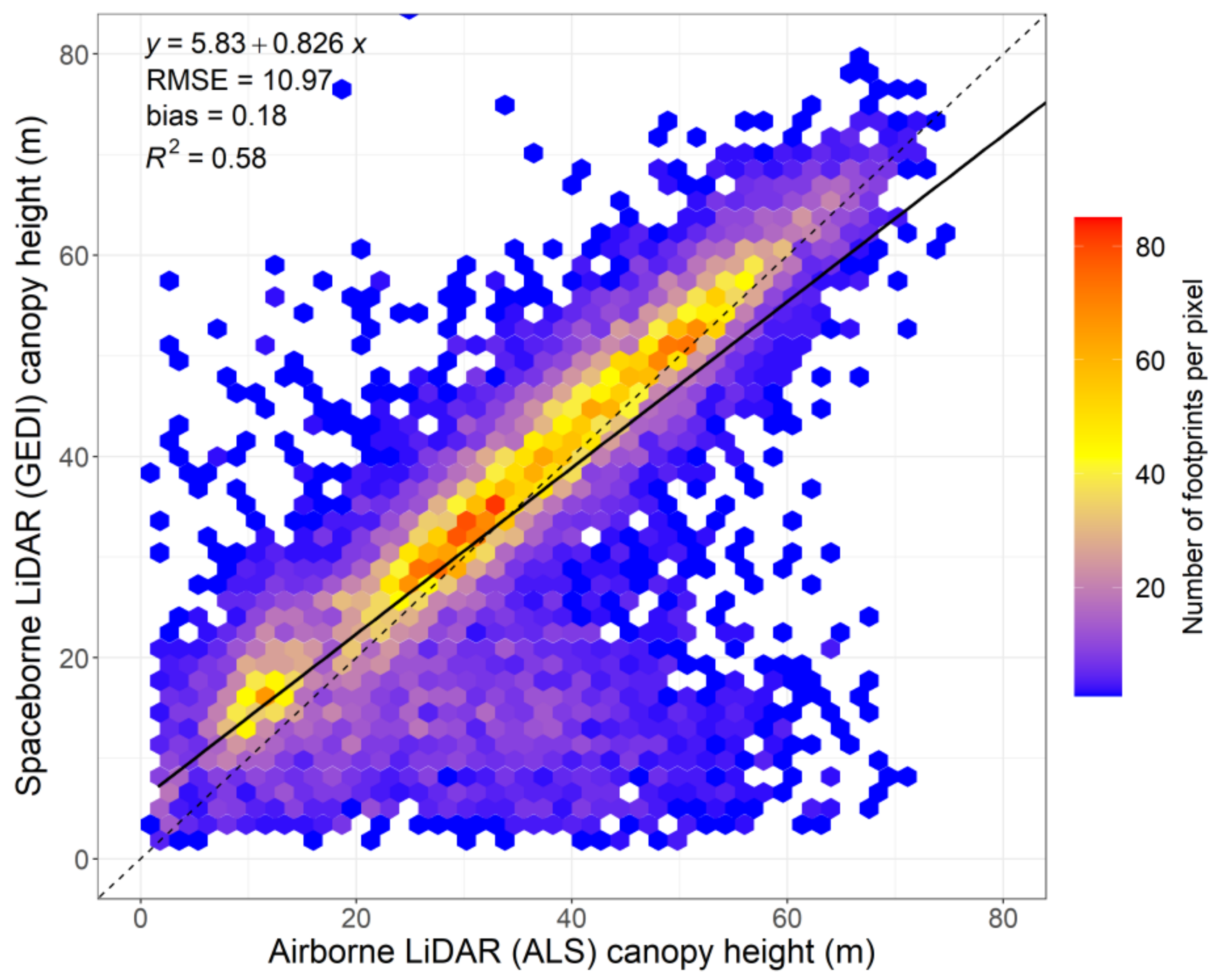
4.2.1. Accuracy of Canopy Height of Individual Footprints

The scatter plot of the canopy height metric between ALS (ALS95) and GEDI (GEDI95) showed consistent error across the footprints sampled (Figure 5), with the highest density of footprints lying close to the 1:1 line. The R2 value is 0.58 which means that 58% of the variation in the GEDI canopy height values can be explained by the ALS values of canopy height. The trend across the canopy height range showed a bias of 0.18 m (%bias −10.01%). The RMSE was 10.97 m (RMSPE 70.02%) and a MAE of 7.05 (MAPE 30.08%).
The overall accuracy of the GEDI canopy height estimates for all the 11,832 footprints is given in Table 3 below, for both beam type combined (power beams or coverage), and separately. When both beam types are considered together, the GEDI canopy height overestimates the reference ALS canopy height with a median value of 1.88 m and a MAD value of 5.35 m. For both beam types, the mean value by which GEDI underestimates ALS is 0.18 m (%bias = −10.01%), and the RMSE is 10.97 m (RMSPE = 70.02%). MAD and MAE for both types of beams are similar (MAD of 5.19 m and 5.58 m and MAE 6.69 and 7.58 for the power and coverage beams, respectively), producing a MAPE difference of 1.29%. The RMSE showed a larger difference (1.63 m), with a RMSPE difference of 18.97%. Despite the larger RMSPE value, the power beam produced a better R2 value of 0.63, with the coverage beam having a greater number of GEDI results under-estimating significantly compared to the power beam.

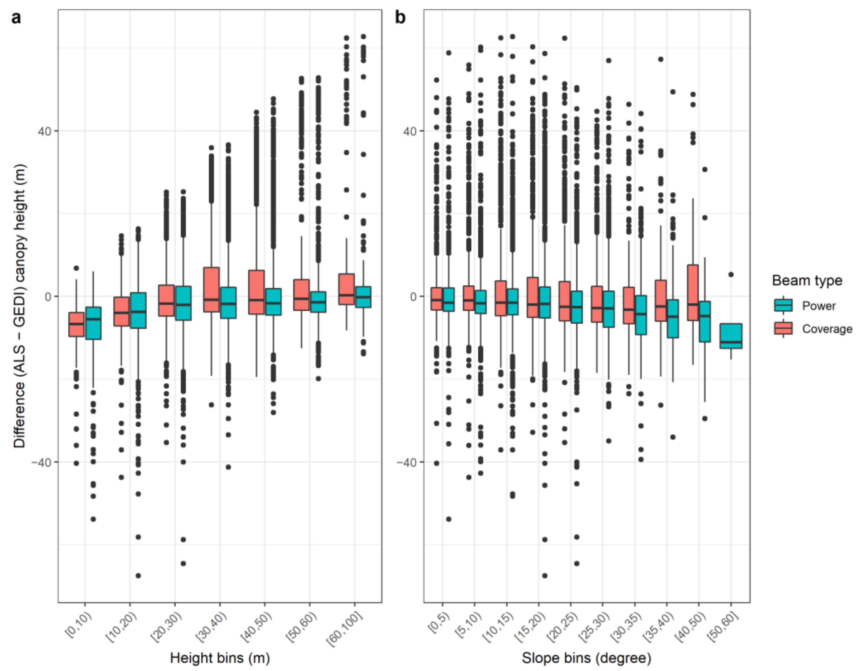
4.2.2. Variation of GEDI Canopy Height Accuracy with Height of the Canopy

The varying difference between ALS and GEDI canopy height (RH95) values for individual footprints across different height classes can be found in Figure 6a. There are some outliers, but the figure shows that the GEDI median value overestimates ALS values for all but the tallest height bin (canopy height > 60 m). The median difference in canopy height between ALS and GEDI peaks at 5.79 m for the 0–10 m height bin and decreases to 3.83 m for the 10–20 m height bin. From the 20–30 m bin upwards, the difference is less than 2 m and decreases with increasing height of the forest canopy. The highest median accuracy is found in the tallest forest canopy height (60–100 m) bin, in which the median of the ALS height is 0.03 m higher than the GEDI height value. The different beam types produced comparable results, with significant overlap in the differences at every height class.
The MAD across the height range did not show any significant trend, with values ranging from 4.05 m to 5.68 m (Table 4). The error variance across the height range was also relatively consistent (MAE ranging from 7.73 m to 6.87 m and RMSE from 10.43 m to 14.16 m). However, this relative consistency in absolute error resulted in an overall decrease in the percentage error with increasing canopy height, with MAPE decreasing from 151.31% to 10.73% and RMSPE decreasing from 256.58 to 22.72, showing that relatively speaking, the GEDI was more accurate when measuring taller forests.

4.2.3. Variation of Canopy Height Accuracy with Slope of Terrain

From Figure 6b, the median GEDI estimate of canopy height exceeds the ALS estimate for all slope classes, and there is an increasing trend in the error in canopy height with increasing slope (increasing median from −1.13 m at 0–5 degrees to −4.22 m at 40–50 degrees, with a similar trend in the mean). The maximum error between ALS and GEDI median estimates of canopy height is 11.11 m for the 50–60 m slope class, but with this class only containing 4 footprints, it may be regarded as an outlier. The MAE was also shown to increase with slope, increasing from 5.62 m to 10.70 m. However, this did not result in a percentage increase with the MAPE (Table 5), indicating that there is a larger abundance of taller forests at greater slopes in the study area. While the overall trend showed an increasing difference with slope, when split into different beam type, the power beam has a greater increase in the error compared to the coverage beam (Figure 6b, indicating that the power beam was more adversely affected at greater slopes than the coverage beam.

4.3. Plant Area Index

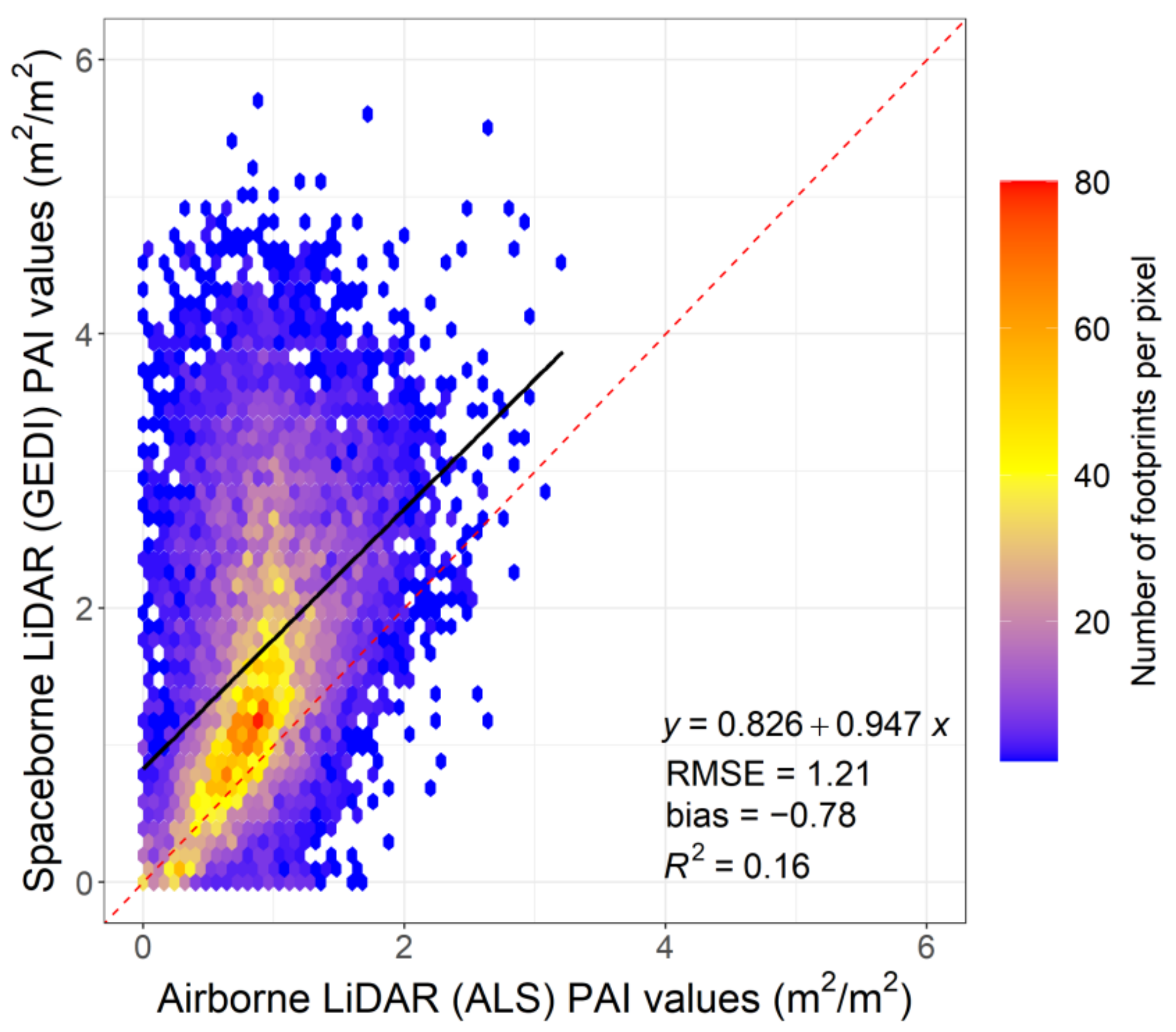
4.3.1. Accuracy of Total PAI of Individual Footprints

The scatter plot of the total PAI metrics between ALS and GEDI shows poor agreement for all the samples in the whole study area (Figure 7), with an R2 value of the linear model of only 0.16, meaning that the ALS PAI values can only explain 16% of the observed variation in GEDI PAI values, along with the trendline of the values sitting significantly above the 1:1 line, with a y-axis intercept of 0.826. The GEDIPAI values are consistently higher than the ALSPAI values, indicating that GEDI generally overestimating the total PAI. The error values produced were also high, with an RMSE of 1.21 m2/m2 (RMSPE = 383.60%) and MAE of 0.88 m2/m2 (MAPE = 144.08%). The different beam types did not improve the overall accuracy (Table 6), with the coverage beam producing a slightly higher correlation (0.20 compared to 0.15), but also had significantly larger errors (increase in RMSPE of 106.92% and MAPE of 32.33%).

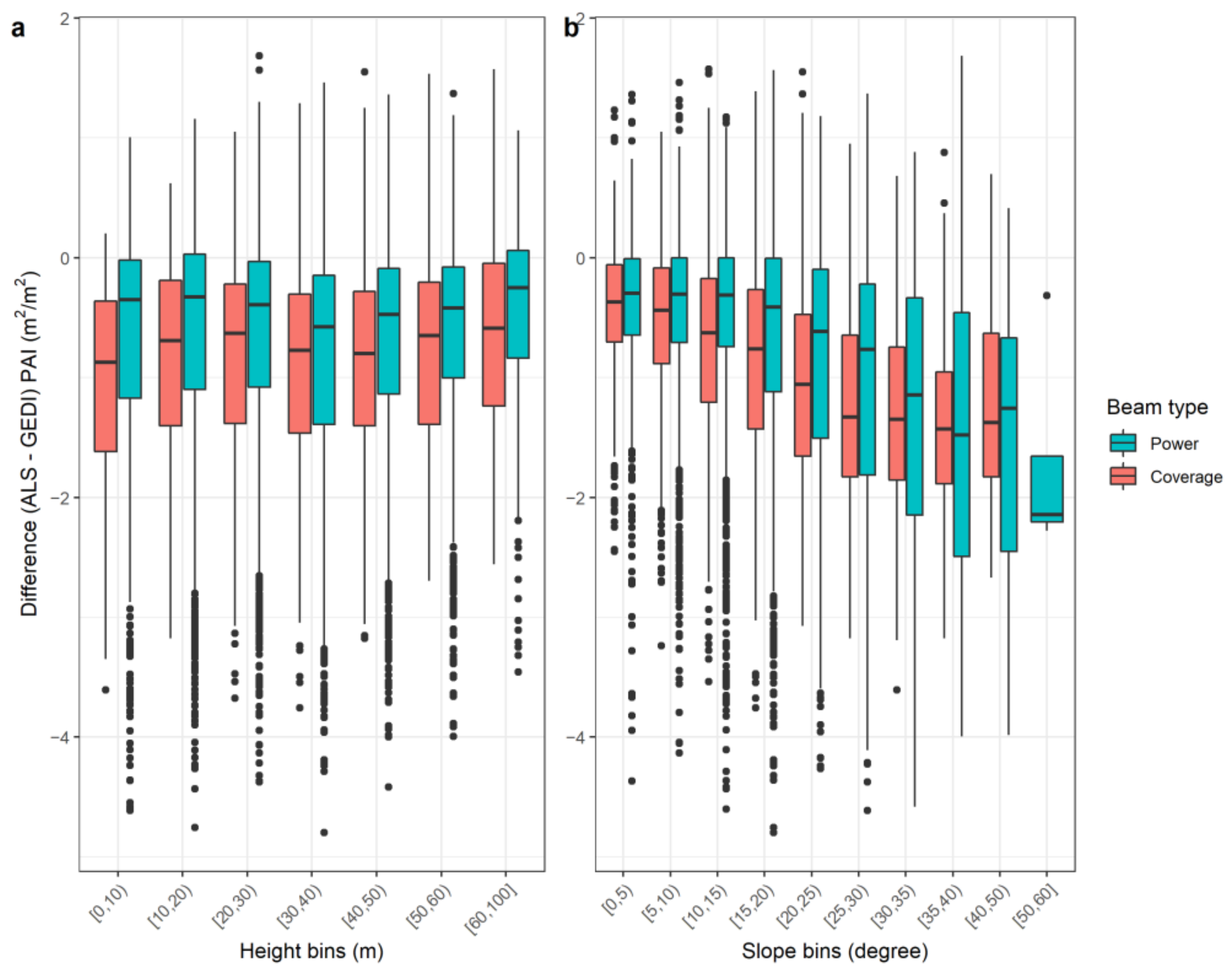
4.3.2. Variation of GEDI PAI Accuracy with Height of the Canopy

For the individual footprints which were grouped into 7 height bins based on their canopy heights derived from airborne LiDAR (ALS95), Figure 8a shows the differences between ALS and GEDI PAI values for all the individual footprints (11,832). As expected from the earlier density plot (Figure 7), GEDI overestimates the ALS values of PAI for all height bins. While the overall performance of the ALS PAI in comparison to the GEDI PAI was poor, the errors did decrease significantly with increasing height (Table 7). With MAPE and RMSPE values decreasing from 659.82% and 1141.78% (0–10 m tall forests), to 67.88% and 96.38% (forests more than 60 m tall). Like the overall comparison of the beam type across the entire dataset, the change in canopy height also did not consistently improve the accuracy of the GEDI values in comparison to the ALS (Figure 8a).

4.3.3. Variation of PAI Accuracy with Slope of Terrain

From Figure 8b, the median GEDI estimate of total PAI exceeds the ALS estimate for all slope classes, with an increasing trend in the difference in PAI values with increasing slope. The maximum absolute difference between ALS and GEDI median estimates of total PAI is 2.14 for the 50–60 m slope class; however, this slope class contains only 4 footprints and may be regarded as an outlier. As the slope increased, the over-estimation of PAI produced by GEDI increased (Table 8). The median difference of −0.32 m2/m2 at 0 to 5 degrees increased to −1.36 m2/m2 at 40 to 50 degrees. The MAE increased from 0.53 m2/m2 to 1.72 m2/m2 across the same range. The MAPE also showed an increase from 84.41% to 211.05%.

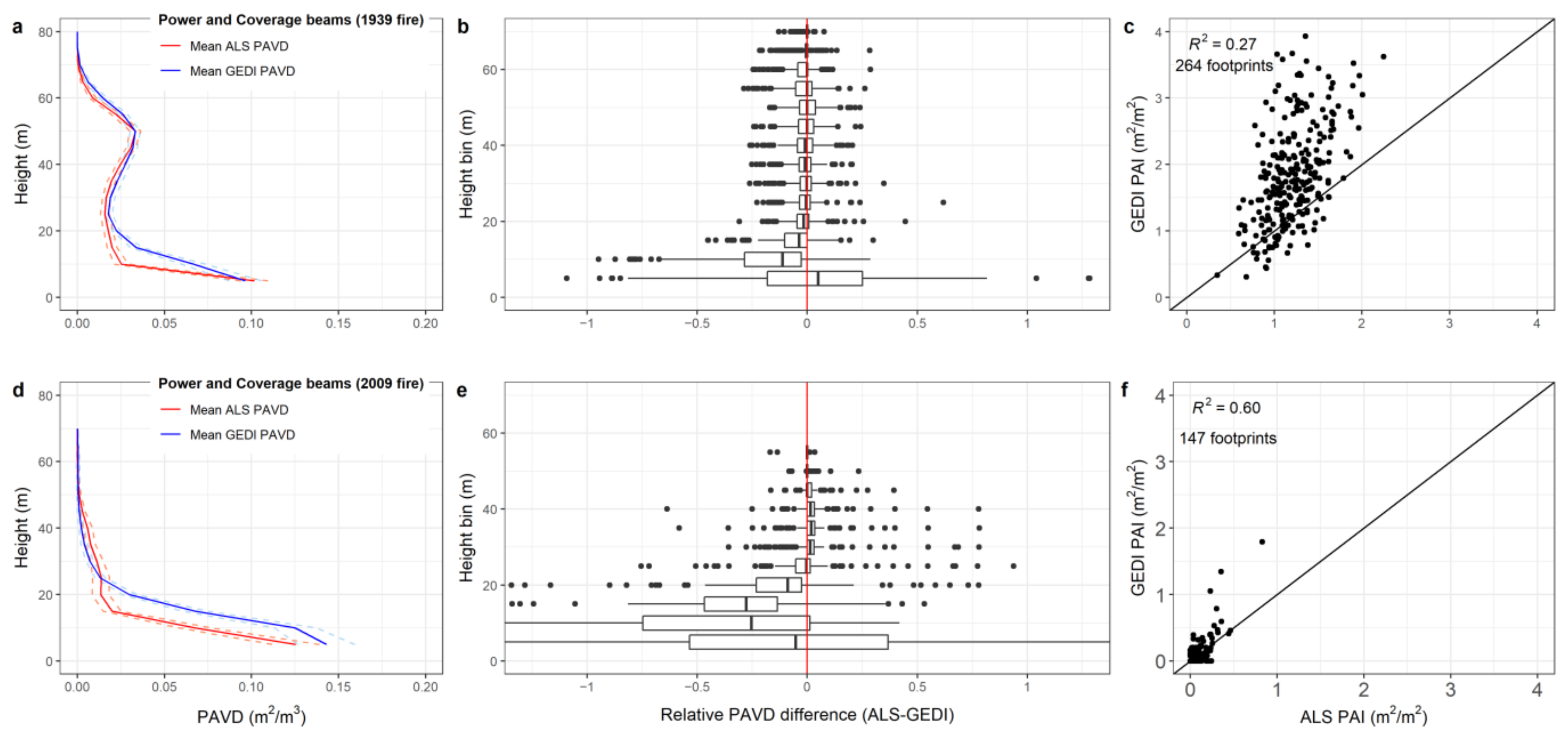
4.4. Analysis of Two Forest Age Classes

The vertical PAVD profile (Figure 9a,b) and scatter plot (Figure 9c) of the total PAI values from GEDI and ALS within the 1939 fire age-class show that GEDI is able to replicate within reasonable ranges the ALS PAVD profile from about 30 m upwards (MAPE decreases from 1171.97% to 103.61%), until the top of the canopy. The highest difference between GEDI and ALS PAVD values occurs at the lower end of the canopy (at 10 m with a median of −0.026). There is also a significant decrease in the RMSPE in this range, from 17,616.88% to 416.49%. The MAD decreased from 0.077 to 0.012 from 5 m to 20 m, remaining around this range for the rest of the vertical profile (0.008 to 0.012). The R2 value of the linear model for total PAI between GEDI and ALS also increased from 0.16 for the entire study area (Figure 7) to 0.27 (Figure 9c).
Similarly, the vertical PAVD profile (Figure 9d,e) and scatter plot (Figure 9f) of the total PAI values from GEDI and ALS for the 2009 fire age-class showed that GEDI is able to replicate the ALS PAVD profile from about 30 m upwards (MAPE decreases from 622.60% to 111.23%), until the top of the canopy. The highest difference between GEDI and ALS PAVD values also occurs at the lower end of the canopy (Table 9). Similar to the 1939, the 2009 fire age-class also saw a significant reduction in RMSPE in this range, from 2749.55% to 177.57%. The R2 value of the linear model for total PAI between GEDI and ALS also increased from 0.16 for the entire study area (Figure 7) to 0.60 (Figure 9f).

5. Discussion

The results of the accuracy assessment of the three forest structure LiDAR metrics of interest from the previous sections are examined in this section in light of the existing literature on similar studies. Relevant studies done thus far on GEDI have focused on assessing the ground elevation and canopy height accuracy in European temperate forests [38]; accuracy of a global 30 m canopy height model extrapolated from GEDI using Landsat optical data [41]; accuracy of extrapolated 1-km resolution contiguous maps of tree height (TH), canopy fraction cover (CFC), PAI, and foliage height diversity (FHD) for the conterminous US (CONUS) using VIIRS satellite data [34], and a study on GEDI simulator performance in eucalypt forests [42].
Of these studies, ref. [38,42] considered the accuracy assessment at GEDI footprint level for canopy height, similar to the methodology in this study. The analysis done in this study assessing total PAI and the vertical foliage profile (VFP; using PAVD) has not been undertaken in the literature to our knowledge. However, there are a couple of studies on PAI and VFP which used full-waveform large footprint LiDAR systems such as the airborne laser vegetation imaging sensor (LVIS) and the space-borne ICESat/GLAS sensor which has similar characteristics to the GEDI [60,78,79]. Therefore, a few pertinent observations will be made on the prominent findings with regard to these studies which used LVIS and GLAS LiDAR data.

5.1. Ground Elevation Effect on Height and Density Attributes

The analysis of the ground elevation showed that the GEDI on average has only a relatively small over-estimation in elevation in comparison to the ALS dataset used (1.28 m). While this is similar in trend to previous studies assessing GEDI elevation, these studies produced smaller over-estimations (Wang et al. [78] = 0.29 m; Quiros et al. [79] = 0.41 m). The high RMSE (10.58 m) was larger than some previous (Quiros et al. [79] = 6.05 m, although they did have values greater than 7.5 in forested and broadleaf areas) studies. However, a recent study by Huettermann et al. [42] had comparably large RMSE values (RMSE > 16 m for raw GEDI), in a similar region (south-eastern Australia). In this concurrent study [42], it was shown that this deviation could be reduced using simulated GEDI (RMSE < 2.35 m). The use of simulated GEDI increased the accuracy of ground elevation measurements and subsequently that of canopy height. The large deviation observed in our ground elevation results is likely to contribute to the large MAD observed in the canopy height (RH95) results. However, despite the large MAD, the low %bias (0.08%), RMSPE (1.76%) and high correlation (1.00) suggest that the overall difference in elevation would not lead to systematic errors when comparing the canopy and PAVD vertical profiles.
While overall the elevation comparison did not show any significant bias (%bias < 5%) across the elevation range, the slope did have an effect. As the slope increased, the under-estimation (in comparison to the ALS elevation values) increased (Figure 4). This effect of slope is consistent with the literature [42]. This error has been found to be worse in dense forests [78]. As our study area contains high density, complex forests, the over-estimation of elevation in our results and increasing deviation with slope is not surprising. Despite this result, the GEDI was still found to over-estimate canopy height (Figure 6b) with increasing slope. This means that the over-estimation in the elevation helped improve the correlation between the GEDI and ALS canopy height results. However, with this effect of slope only increasing significantly after ~30 degrees, the slope effect on the canopy height, PAI, and PAVD is likely to only affect a small subset of the footprints in the study area, with the trend in the deviation not reducing the accuracy of the analysis for these forest structural metrics.

5.2. Can GEDI Estimate ALS-Based Canopy Height?

Adam et al. [38] assessed the accuracy of GEDI estimates of canopy height at the individual footprint level, although they acknowledged the considerably poor geolocation accuracy of the GEDI Version 1 data that they used (1σ of 10–20 m). For this study, the Version 2 GEDI data with better geolocation accuracy (1σ of 10 m) were used.
Another difference is that [38] took the maximum value of the GEDI footprint of the canopy height model (CHM) generated from the ALS data, for comparing with the GEDI RH100 relative height metric, whereas in this study, the selected canopy height metric (RH95) of the ALS data (ALS95) was derived from the pseudo-waveform generated from the ALS point-cloud data, which was then compared with the RH95 metric from the GEDI data (GEDI95). This approach of emulating full waveform data from discrete return point-cloud airborne LiDAR data was found to provide a robust comparison of stand canopy metrics to reference data by Coops et al. [26] and also used by Roy et al. [66] in their assessment of the impacts of GEDI’s geolocation uncertainty.
The overall median of the differences in canopy height (ALS95, GEDI95) (Table 3) is −1.88 m with a median absolute difference (MAD) of 5.35 m, which is more than that found by [38] for the Thuringian temperate forest region in Germany, viz. a median of −0.23 m, with a MAD of 3.17 m. The higher canopy height difference could be due to the time difference between the acquisition of the two datasets (ALS in 2015-16 and GEDI in 2018) of about 3 years.
The mean growth rate of eucalyptus spp. in this is region is around 0.7 m/year [80], which could explain much of the difference in canopy heights between the two sensors (total growth in canopy height of approximately 2.1 m, for the approximately 3 years difference in time of acquisition between the ALS and GEDI data). This would give an actual median canopy height difference of 1.88 m −2.1 m = −0.22 m, which is very close to the median value of the differences between ALS and GEDI (viz. −0.23 m) found by Adam et al. [38].
Our results for the actual GEDI data are similar to those of Huettermann et al. [42]. However, the GEDI proved better at identifying canopy heights in tall forests in our study. The range of forest types used by Huetterman et al. [42] provided a more structurally diverse dataset than this paper focusing predominantly on canopy height, and notably, they found better correspondence between ALS and GEDI in shorter forests.
Kutchartt et al. [81]and Liu et al. [39] report that power beams provide more accuracy for canopy height retrieval. However, there is an absolute difference of 0.39 m in the corresponding median values of canopy height errors for the power and coverage beams, with the power beam exhibiting a higher median error of −2.03 (Table 3). This is surprising given that in dense forests, the coverage beams are expected to perform worse, having less laser energy to penetrate to the ground, which is why generally the power beams are recommended to be used [55].
Finally, the 3–4-year time difference between the ALS and GEDI missions introduces a potential source of error. For canopy height, this relates to stand growth dynamics. Our finding that GEDI significantly overestimated height for trees <20 m may be in part a function of growth rates. Annual increases in height for E. regnans forest range from 1.6 m year−1 (~20-year-old stand) to less than 0.4 m year−1 for mature (80+ year-old) trees [82]. This may account for GEDI overestimation of RH95 in Figure 5 for trees <20 m, because growth rates are higher in younger stands.

5.3. Can GEDI Estimate Total PAI Accurately?

The density plot (Figure 7) of the total PAI values from all the individual footprints (11,832) for ALS (ALSPAI) and GEDI (GEDIPAI) shows a low R2 value of 0.16. One possible source of the error could be the poor geolocation accuracy of individual footprints which have an uncertainty (1σ) of about ±10 m. This may be highly significant in the study area, which has a high level of variability in the vegetation structure within very short distances [27,28].
The error in the PAI also seems to be decreasing as the value of the canopy height classes or bins increase. This could be related to the difference in the years between data capture for GEDI and ALS, as we would expect the younger and shorter forests to change more in this timeframe given that they are likely to be growing at a faster rate. Thus, much of the observed difference (the over-estimation by GEDI) in the values of ALSPAI and GEDIPAI may be caused by the growth that has taken place in the forest during the 3 years since the ALS data were captured in 2015–2016; the GEDIPAI may thus be closer to the reference value than is shown by the observed discrepancy. Conversely, this may be a function of the complex structure in mountain ash forests.

5.4. Can GEDI Represent the Vertical Canopy Profile Accurately?

For the 1939 age-class, the PAVD vertical profile (Figure 9a) shows a marked improvement in the agreement between the ALS and GEDI values of PAVD once the canopy height of the samples (i.e., the height bins) exceeds approximately 30 m. Below this height threshold, the GEDI PAVD profile does not seem to be following the variation in the ALS PAVD profile well.
Therefore, GEDI does not appear to be accurate in the understory layer, i.e., below a canopy height of about 30 m. This is not consistent with the PAI pattern observed by Tang et al. [60] in a tropical forest in South America using the LVIS sensor and destructive sampling towers for reference data. Their finding was that the PAI vertical profile of the full-waveform LVIS sensor replicated the reference dataset without any specific height dependence or threshold. These contrasting results are curious. Our hypothesis is that the complex multi-strata understory in the ash forests posed a problem for the GEDI. However, the same might be expected for a tropical forest. This would seem to be an area for further research.

5.5. Operational Use of GEDI in South-East Australian Forests

The choice of which LiDAR platform to use is guided by the spatio-temporal resolution of data required for the application. Mature forests that have slower growth rates and little disturbance may not require repeat observations for some studies. ALS can be appropriate for many applications (e.g., [27,83]). Studies that require individual tree identification can require higher resolution data capture than either ALS or GEDI (see [12]).
A significant advantage of GEDI is its free availability, meaning that local jurisdictions, governments, and community organizations that cannot afford ALS data capture now have a readily accessible source of data on forest structure and resources. Although ALS is more accurate after large disturbance events such as wildfire or timber harvesting have occurred, the ALS dataset becomes quickly outdated and not representative of the forest’s current state.
Additionally, younger forests grow quickly and dynamically, so having a repeat measure is invaluable for monitoring forest growth rates. This is not realistic with an ALS-based approach for various reasons such as cost and logistics. These challenges of ALS were evident in this project, wherein the ALS data were collected in 2015–2016 and it has not been flown since. Spectral remote sensing products that are in common use are often based on using ‘greenness’ as a metric. This is problematic because of the uncertainty surrounding where the measured recovery is occurring structurally (e.g., understory regrowth, epicormic growth, or canopy recovery) after disturbance. The use of simulated GEDI, e.g., ([42,84]), is proposed as a method to both improve canopy height capture, and provides a more robust geolocation for repeat measures. Whether simulation improves other structural metrics is not well tested at this time.
The variable results reported here on PAI and PAVD suggest that some applications, such as fuel accumulation, LAI use in evapotranspiration models, or biomass growth may be beyond the current GEDI (at least as we have used it). However, it may be useable in a relative sense, and certainly any application using canopy height and PAVD of the overstorey and upper strata is confirmed.

5.6. Limitations of the Study

There is an inherent difference in terms of the full waveform vs. discrete return nature of the GEDI and ALS data acquisition modes, respectively. This has been addressed by deriving the canopy height metrics after simulating full waveform data from the ALS point-cloud data, which would help to minimize the discrepancies due to this difference in data acquisition mode [40,62,64,66].
The errors due to geo-location uncertainty in GEDI have no significant impact on the findings. The version 2 data product used here is within the mission design requirement of a geolocation error of 10 m (1σ). Roy et al. [66] and Liu et al. [39] examined the impact of this level of geolocation uncertainty on the reliability of canopy height estimation from GEDI.
As discussed above, a limitation of our study is the time between ALS (2015–2016) and GEDI data capture (2019), which may increase discrepancies between the sensors for all metrics. While growth rates of E. regnans are reasonably well known, there is less understanding of the dynamics of understory species [82]. We cannot ascribe errors arising from this source currently.

5.7. Future Research

Future studies could use more customized algorithms to process the raw GEDI L1B waveforms to get more accurate total PAI and vertical profile metrics. These algorithms could use more accurate values of the canopy to ground reflectivity ratio ( ρ v ρ g ) specific for the Australian temperate forest biome instead of the default value applied in the standard GEDI L2B data product [55].
Based upon the findings of this study, estimation of mean annual changes in forest ecosystem structure at the stand and landscape scale using GEDI data can be carried out. This could be used in applications such as aboveground biomass stock estimation, assessing the impacts of climate change and forest disturbances on water supplies and critical biodiversity habitat.

6. Conclusions

At the landscape scale, for 11,832 footprints, around 58% of the observed variation in the ALS canopy height values can be explained by the GEDI values of canopy height. The RMSE is 10.97 m (RMSPE of 70.02%) and the bias is 0.18 m (%bias of −10.02%). The GEDI overestimates the canopy height with a median value of 1.88 m and median absolute difference (MAD) of 5.35 m. The coverage beams are found to have comparable accuracy to the power beams. The accuracy improves for canopy heights above 20 m and decreases consistently for increasing terrain slope bins.
For the total PAI values, the ALS and GEDI values show poor agreement, with only 16% of the observed variation in ALS PAI values explained by the GEDI values. The RMSE is 1.21 m2/m2 and the bias is 0.87 m2/m2. GEDI generally overestimates the total PAI with a median value of −0.55 m and MAD value of 0.78 m. The accuracy of the power beams is found to be better than the coverage beams for total PAI. The absolute accuracy is low and remains stable (median value of ~0.50) for all canopy heights, and only improves significantly to 0.39 for a tall canopy with heights above 60 m. For increasing terrain slopes, the absolute accuracy degrades consistently from a median value of 0.32 for the lowest slope bin to a maximum of 2.13 for the highest slope bin. For the vertical PAVD profile, the error is found to be significant below a 30 m canopy height threshold. Above this threshold, the GEDI replicates the reference ALS vertical PAVD profile well.
We conclude that GEDI is appropriate for capturing PAI at the canopy level in tall forests, with most of the error or over-estimation near the forest floor. Within the limitations of the study discussed above, it would appear that space-borne LiDAR (GEDI) performs well in quantifying the canopy height and vertical structure of tall eucalyptus forests of south-eastern Australia, especially for characterizing the over-story canopy structure.

Author Contributions

Conceptualization, S.D., G.J.S. and P.N.J.L.; data curation, S.D. and C.S.L.; formal analysis, S.D., C.S.L., A.I., T.P.B., G.J.S. and P.N.J.L.; funding acquisition, G.J.S. and P.N.J.L.; methodology, S.D., C.S.L., T.P.B., A.I., G.J.S. and P.N.J.L.; software, S.D., C.S.L. and T.P.B.; supervision, G.J.S. and P.N.J.L.; validation, S.D., C.S.L., T.P.B., A.I., G.J.S. and P.N.J.L.; visualization, A.I., S.D. and C.S.L.; writing—original draft, S.D.; writing—review and editing, S.D., C.S.L., T.P.B., A.I., G.J.S. and P.N.J.L. All authors have read and agreed to the published version of the manuscript.

Funding

This work was supported by the Integrated Forest Ecosystem Research program, funded by the Victorian Department of Environment, Land, Water, and Planning (DELWP) (grant number: 094687).

Data Availability Statement

Not applicable.

Acknowledgments

We thank the Department of Environment, Land, Water, and Planning (DELWP), Australia, and NASA for providing the airborne LiDAR and GEDI data of the Central Highlands used in this study. Many thanks also to Aaron Heap for the processed shapefiles of the fire-affected mountain ash areas within the study area, which were used in the case-study analysis. Additionally, thanks to Raphael Trouve who supplied the ALS DEM which was used for the elevation analysis.

Conflicts of Interest

The authors declare no conflict of interest.

References

  1. Lefsky, M.A.; Cohen, W.B.; Acker, S.A.; Parker, G.G.; Spies, T.A.; Harding, D. Lidar Remote Sensing of the Canopy Structure and Biophysical Properties of Douglas-Fir Western Hemlock Forests. Remote Sens. Environ. 1999, 70, 339–361. [Google Scholar] [CrossRef]
  2. Riaño, D.; Valladares, F.; Condés, S.; Chuvieco, E. Estimation of Leaf Area Index and Covered Ground from Airborne Laser Scanner (Lidar) in Two Contrasting Forests. Agric. For. Meteorol. 2004, 124, 269–275. [Google Scholar] [CrossRef]
  3. Shugart, H.H.; Saatchi, S.; Hall, F.G. Importance of Structure and Its Measurement in Quantifying Function of Forest Ecosystems. J. Geophys. Res. Biogeosci. 2010, 115, G00E13. [Google Scholar] [CrossRef]
  4. Sinha, S.; Jeganathan, C.; Sharma, L.K.; Nathawat, M.S. A Review of Radar Remote Sensing for Biomass Estimation. Int. J. Environ. Sci. Technol. 2015, 12, 1779–1792. [Google Scholar] [CrossRef] [Green Version]
  5. Naesset, E. Determination of Mean Tree Height of Forest Stands Using Airborne Laser Scanner Data. ISPRS J. Photogramm. Remote Sens. 1997, 52, 49–56. [Google Scholar] [CrossRef]
  6. Nilsson, M. Estimation of Tree Heights and Stand Volume Using an Airborne Lidar System. Remote Sens. Environ. 1996, 56, 1–7. [Google Scholar] [CrossRef]
  7. Lefsky, M.A.; Harding, D.; Cohen, W.B.; Parker, G.; Shugart, H.H. Surface Lidar Remote Sensing of Basal Area and Biomass in Deciduous Forests of Eastern Maryland, USA. Remote Sens. Environ. 1999, 67, 83–98. [Google Scholar] [CrossRef]
  8. Lefsky, M.A. Application of Lidar Remote Sensing to the Estimation of Forest Canopy and Stand Structure. Ph.D. Thesis, University of Virginia, Charlottesville, VA, USA, 1997. Volume 130. [Google Scholar]
  9. Lefsky, M.A.; Harding, D.J.; Keller, M.; Cohen, W.B.; Carabajal, C.C.; Del Bom Espirito-Santo, F.; Hunter, M.O.; de Oliveira, R., Jr. Estimates of Forest Canopy Height and Aboveground Biomass Using ICESat. Geophys. Res. Lett. 2005, 32. [Google Scholar] [CrossRef] [Green Version]
  10. Lefsky, M.A.; Cohen, W.B.; Parker, G.G.; Harding, D.J. Lidar Remote Sensing for Ecosystem Studies: Lidar, an Emerging Remote Sensing Technology That Directly Measures the Three-Dimensional Distribution of Plant Canopies, Can Accurately Estimate Vegetation Structural Attributes and Should Be of Particular Inte. Bioscience 2002, 52, 19–30. [Google Scholar] [CrossRef]
  11. Magnussen, S.; Boudewyn, P. Derivations of Stand Heights from Airborne Laser Scanner Data with Canopy-Based Quantile Estimators. Can. J. For. Res. 1998, 28, 1016–1031. [Google Scholar] [CrossRef]
  12. Jaskierniak, D.; Lucieer, A.; Kuczera, G.; Turner, D.; Lane, P.N.J.; Benyon, R.G.; Haydon, S. Individual Tree Detection and Crown Delineation from Unmanned Aircraft System (UAS) LiDAR in Structurally Complex Mixed Species Eucalypt Forests. ISPRS J. Photogramm. Remote Sens. 2021, 171, 171–187. [Google Scholar] [CrossRef]
  13. McColl-Gausden, S.C.; Bennett, L.T.; Clarke, H.G.; Ababei, D.A.; Penman, T.D. The Fuel–Climate–Fire Conundrum: How Will Fire Regimes Change in Temperate Eucalypt Forests under Climate Change? Glob. Chang. Biol. 2022. [Google Scholar] [CrossRef]
  14. Keeley, J.E.; Syphard, A.D. Climate Change and Future Fire Regimes: Examples from California. Geosciences 2016, 6, 37. [Google Scholar] [CrossRef] [Green Version]
  15. Cary, G.J. Importance of a Changing Climate for Fire Regimes in Australia. In Flammable Australia: The Fire Regimes and Biodiversity of a Continent; Bradstock, R.A., Williams, J.E., Gill, M.A., Eds.; Cambridge University Press: Cambridge, UK, 2002; pp. 26–46. [Google Scholar]
  16. Liu, Z.; Wimberly, M.C. Direct and Indirect Effects of Climate Change on Projected Future Fire Regimes in the Western United States. Sci. Total Environ. 2016, 542, 65–75. [Google Scholar] [CrossRef] [PubMed] [Green Version]
  17. Goetz, S.; Dubayah, R. Advances in Remote Sensing Technology and Implications for Measuring and Monitoring Forest Carbon Stocks and Change. Carbon Manag. 2011, 2, 231–244. [Google Scholar] [CrossRef]
  18. Bustamante, M.M.C.; Roitman, I.; Aide, T.M.; Alencar, A.; Anderson, L.O.; Aragão, L.; Asner, G.P.; Barlow, J.; Berenguer, E.; Chambers, J. Toward an Integrated Monitoring Framework to Assess the Effects of Tropical Forest Degradation and Recovery on Carbon Stocks and Biodiversity. Glob. Chang. Biol. 2016, 22, 92–109. [Google Scholar] [CrossRef] [PubMed]
  19. Asner, G.P. Tropical Forest Carbon Assessment: Integrating Satellite and Airborne Mapping Approaches. Environ. Res. Lett. 2009, 4, 34009. [Google Scholar] [CrossRef]
  20. Dubayah, R.; Blair, J.B.; Goetz, S.; Fatoyinbo, L.; Hansen, M.; Healey, S.; Hofton, M.; Hurtt, G.; Kellner, J.; Luthcke, S.; et al. The Global Ecosystem Dynamics Investigation: High-Resolution Laser Ranging of the Earth’s Forests and Topography. Sci. Remote Sens. 2020, 1, 100002. [Google Scholar] [CrossRef]
  21. Hall, F.G.; Bergen, K.; Blair, J.B.; Dubayah, R.; Houghton, R.; Hurtt, G.; Kellndorfer, J.; Lefsky, M.; Ranson, J.; Saatchi, S. Characterizing 3D Vegetation Structure from Space: Mission Requirements. Remote Sens. Environ. 2011, 115, 2753–2775. [Google Scholar] [CrossRef] [Green Version]
  22. Bergen, K.M.; Goetz, S.J.; Dubayah, R.O.; Henebry, G.M.; Hunsaker, C.T.; Imhoff, M.L.; Nelson, R.F.; Parker, G.G.; Radeloff, V.C. Remote Sensing of Vegetation 3-D Structure for Biodiversity and Habitat: Review and Implications for Lidar and Radar Spaceborne Missions. J. Geophys. Res. Biogeosci. 2009, 114. [Google Scholar] [CrossRef] [Green Version]
  23. Aber, J.D. Foliage-height Profiles and Succession in Northern Hardwood Forests. Ecology 1979, 60, 18–23. [Google Scholar] [CrossRef]
  24. Gower, S.T.; Norman, J.M. Rapid Estimation of Leaf Area Index in Conifer and Broad-Leaf Plantations. Ecology 1991, 72, 1896–1900. [Google Scholar] [CrossRef]
  25. Baret, F.; Weiss, M.; Lacaze, R.; Camacho, F.; Makhmara, H.; Pacholcyzk, P.; Smets, B. GEOV1: LAI and FAPAR Essential Climate Variables and FCOVER Global Time Series Capitalizing over Existing Products. Part1: Principles of Development and Production. Remote Sens. Environ. 2013, 137, 299–309. [Google Scholar] [CrossRef]
  26. Coops, N.C.; Hilker, T.; Wulder, M.A.; St-Onge, B.; Newnham, G.; Siggins, A.; Trofymow, J.A. Estimating Canopy Structure of Douglas-Fir Forest Stands from Discrete-Return LiDAR. Trees Struct. Funct. 2007, 21, 295–310. [Google Scholar] [CrossRef] [Green Version]
  27. Jaskierniak, D.; Lane, P.N.J.; Robinson, A.; Lucieer, A. Extracting LiDAR Indices to Characterise Multilayered Forest Structure Using Mixture Distribution Functions. Remote Sens. Environ. 2011, 115, 573–585. [Google Scholar] [CrossRef]
  28. Mitchell, P.J.; Benyon, R.G.; Lane, P.N.J. Responses of Evapotranspiration at Different Topographic Positions and Catchment Water Balance Following a Pronounced Drought in a Mixed Species Eucalypt Forest, Australia. J. Hydrol. 2012, 440–441, 62–74. [Google Scholar] [CrossRef]
  29. Fedrigo, M.; Newnham, G.J.; Coops, N.C.; Culvenor, D.S.; Bolton, D.K.; Nitschke, C.R. Predicting Temperate Forest Stand Types Using Only Structural Profiles from Discrete Return Airborne Lidar. ISPRS J. Photogramm. Remote Sens. 2018, 136, 106–119. [Google Scholar] [CrossRef]
  30. Silva, C.A.; Duncanson, L.; Hancock, S.; Neuenschwander, A.; Thomas, N.; Hofton, M.; Fatoyinbo, L.; Simard, M.; Marshak, C.Z.; Armston, J. Fusing Simulated GEDI, ICESat-2 and NISAR Data for Regional Aboveground Biomass Mapping. Remote Sens. Environ. 2021, 253, 112234. [Google Scholar] [CrossRef]
  31. Liu, X.; Su, Y.; Hu, T.; Yang, Q.; Liu, B.; Deng, Y.; Tang, H.; Tang, Z.; Fang, J.; Guo, Q. Neural Network Guided Interpolation for Mapping Canopy Height of China’s Forests by Integrating GEDI and ICESat-2 Data. Remote Sens. Environ. 2022, 269, 112844. [Google Scholar] [CrossRef]
  32. Lefsky, M.A.; Keller, M.; Pang, Y.; De Camargo, P.B.; Hunter, M.O. Revised Method for Forest Canopy Height Estimation from Geoscience Laser Altimeter System Waveforms. J. Appl. Remote Sens. 2007, 1, 13537. [Google Scholar]
  33. Qi, W.; Dubayah, R.O. Combining Tandem-X InSAR and Simulated GEDI Lidar Observations for Forest Structure Mapping. Remote Sens. Environ. 2016, 187, 253–266. [Google Scholar] [CrossRef]
  34. Spracklen, B.; Spracklen, D. V Determination of Structural Characteristics of Old-Growth Forest in Ukraine Using Spaceborne LiDAR. Remote Sens. 2021, 13, 1233. [Google Scholar] [CrossRef]
  35. Rishmawi, K.; Huang, C.; Zhan, X. Monitoring Key Forest Structure Attributes across the Conterminous United States by Integrating GEDI LiDAR Measurements and VIIRS Data. Remote Sens. 2021, 13, 442. [Google Scholar] [CrossRef]
  36. Li, W.; Niu, Z.; Shang, R.; Qin, Y.; Wang, L.; Chen, H. High-Resolution Mapping of Forest Canopy Height Using Machine Learning by Coupling ICESat-2 LiDAR with Sentinel-1, Sentinel-2 and Landsat-8 Data. Int. J. Appl. Earth Obs. Geoinf. 2020, 92, 102163. [Google Scholar] [CrossRef]
  37. Jiang, F.; Zhao, F.; Ma, K.; Li, D.; Sun, H. Mapping the Forest Canopy Height in Northern China by Synergizing ICESat-2 with Sentinel-2 Using a Stacking Algorithm. Remote Sens. 2021, 13, 1535. [Google Scholar] [CrossRef]
  38. Adam, M.; Urbazaev, M.; Dubois, C.; Schmullius, C. Accuracy Assessment of GEDI Terrain Elevation and Canopy Height Estimates in European Temperate Forests: Influence of Environmental and Acquisition Parameters. Remote Sens. 2020, 12, 3948. [Google Scholar] [CrossRef]
  39. Liu, A.; Cheng, X.; Chen, Z. Performance Evaluation of GEDI and ICESat-2 Laser Altimeter Data for Terrain and Canopy Height Retrievals. Remote Sens. Environ. 2021, 264, 112571. [Google Scholar] [CrossRef]
  40. Guerra-Hernández, J.; Pascual, A. Using GEDI Lidar Data and Airborne Laser Scanning to Assess Height Growth Dynamics in Fast-Growing Species: A Showcase in Spain. For. Ecosyst. 2021, 8, 14. [Google Scholar] [CrossRef]
  41. Potapov, P.; Li, X.; Hernandez-Serna, A.; Tyukavina, A.; Hansen, M.C.; Kommareddy, A.; Pickens, A.; Turubanova, S.; Tang, H.; Silva, C.E. Mapping Global Forest Canopy Height through Integration of GEDI and Landsat Data. Remote Sens. Environ. 2021, 253, 112165. [Google Scholar] [CrossRef]
  42. Huettermann, S.; Jones, S.; Soto-Berelov, M.; Hislop, S. Intercomparison of Real and Simulated GEDI Observations across Sclerophyll Forests. Remote Sens. 2022, 14, 2096. [Google Scholar] [CrossRef]
  43. Nyman, P.; Metzen, D.; Hawthorne, S.N.D.; Duff, T.J.; Inbar, A.; Lane, P.N.J.; Sheridan, G.J. Evaluating Models of Shortwave Radiation below Eucalyptus Canopies in SE Australia. Agric. For. Meteorol. 2017, 246, 51–63. [Google Scholar] [CrossRef]
  44. Brown, T.P.; Inbar, A.; Duff, T.J.; Burton, J.; Noske, P.J.; Lane, P.N.J.; Sheridan, G.J. Forest Structure Drives Fuel Moisture Response across Alternative Forest States. Fire 2021, 4, 48. [Google Scholar] [CrossRef]
  45. Wilkes, P.; Jones, S.D.; Suarez, L.; Mellor, A.; Woodgate, W.; Soto-Berelov, M.; Haywood, A.; Skidmore, A.K. Mapping Forest Canopy Height across Large Areas by Upscaling ALS Estimates with Freely Available Satellite Data. Remote Sens. 2015, 7, 12563–12587. [Google Scholar] [CrossRef] [Green Version]
  46. Lim, K.; Treitz, P.; Wulder, M.; St-Onge, B.; Flood, M. LiDAR Remote Sensing of Forest Structure. Prog. Phys. Geogr. 2003, 27, 88–106. [Google Scholar] [CrossRef] [Green Version]
  47. Monsi, M.; Saeki, T. On the Factor Light in Plant Communities and Its Importance for Matter Production. Ann. Bot. 2005, 95, 549. [Google Scholar] [CrossRef] [Green Version]
  48. Cawson, J.G.; Duff, T.J.; Tolhurst, K.G.; Baillie, C.C.; Penman, T.D. Fuel Moisture in Mountain Ash Forests with Contrasting Fire Histories. For. Ecol. Manag. 2017, 400, 568–577. [Google Scholar] [CrossRef]
  49. Edwards, D.P.; Fisher, B.; Boyd, E. Protecting Degraded Rainforests: Enhancement of Forest Carbon Stocks under REDD+. Conserv. Lett. 2010, 3, 313–316. [Google Scholar] [CrossRef]
  50. Griebel, A.; Bennett, L.T.; Culvenor, D.S.; Newnham, G.J.; Arndt, S.K. Reliability and Limitations of a Novel Terrestrial Laser Scanner for Daily Monitoring of Forest Canopy Dynamics. Remote Sens. Environ. 2015, 166, 205–213. [Google Scholar] [CrossRef]
  51. Karna, K.Y.; Penman, D.T.; Aponte, C.; Bennett, T.L. Assessing Legacy Effects of Wildfires on the Crown Structure of Fire-Tolerant Eucalypt Trees Using Airborne LiDAR Data. Remote Sens. 2019, 11, 2433. [Google Scholar] [CrossRef] [Green Version]
  52. Wilkes, P.; Jones, S.D.; Suarez, L.; Haywood, A.; Mellor, A.; Woodgate, W.; Soto-Berelov, M.; Skidmore, A.K. Using Discrete-Return Airborne Laser Scanning to Quantify Number of Canopy Strata across Diverse Forest Types. Methods Ecol. Evol. 2016, 7, 700–712. [Google Scholar] [CrossRef]
  53. Woodgate, W.; Disney, M.; Armston, J.D.; Jones, S.D.; Suarez, L.; Hill, M.J.; Wilkes, P.; Soto-Berelov, M.; Haywood, A.; Mellor, A. An Improved Theoretical Model of Canopy Gap Probability for Leaf Area Index Estimation in Woody Ecosystems. For. Ecol. Manag. 2015, 358, 303–320. [Google Scholar] [CrossRef]
  54. Wilkes, P.; Jones, S.D.; Suarez, L.; Haywood, A.; Woodgate, W.; Soto-Berelov, M.; Mellor, A.; Skidmore, A.K. Understanding the Effects of ALS Pulse Density for Metric Retrieval across Diverse Forest Types. Photogramm. Eng. Remote Sens. 2015, 81, 625–635. [Google Scholar] [CrossRef]
  55. Tang, H.; Armston, J.; Dubayah, R. Algorithm Theoretical Basis Document (ATBD) for GEDI L2B Footprint Canopy Cover and Vertical Profile Metrics; Goddard Space Flight Center: Greenbelt, MD, USA, 2019. [Google Scholar]
  56. Hofton, M.; Blair, J.B.; Story, S.; Yi, D. Algorithm Theoretical Basis Document (ATBD) for GEDI Transmit and Receive Waveform Processing for L1 and L2 Products; University of Maryland: College Park, MA, USA, 2020. [Google Scholar]
  57. Ni-Meister, W.; Jupp, D.L.B.; Dubayah, R. Modeling Lidar Waveforms in Heterogeneous and Discrete Canopies. IEEE Trans. Geosci. Remote Sens. 2001, 39, 1943–1958. [Google Scholar] [CrossRef] [Green Version]
  58. Armston, J.; Disney, M.; Lewis, P.; Scarth, P.; Phinn, S.; Lucas, R.; Bunting, P.; Goodwin, N. Direct Retrieval of Canopy Gap Probability Using Airborne Waveform Lidar. Remote Sens. Environ. 2013, 134, 24–38. [Google Scholar] [CrossRef]
  59. Pisek, J.; Govind, A.; Arndt, S.K.; Hocking, D.; Wardlaw, T.J.; Fang, H.; Matteucci, G.; Longdoz, B. Intercomparison of Clumping Index Estimates from POLDER, MODIS, and MISR Satellite Data over Reference Sites. ISPRS J. Photogramm. Remote Sens. 2015, 101, 47–56. [Google Scholar] [CrossRef]
  60. Tang, H.; Dubayah, R.; Swatantran, A.; Hofton, M.; Sheldon, S.; Clark, D.B.; Blair, B. Retrieval of Vertical LAI Profiles over Tropical Rain Forests Using Waveform Lidar at La Selva, Costa Rica. Remote Sens. Environ. 2012, 124, 242–250. [Google Scholar] [CrossRef]
  61. Zhao, K.; Popescu, S. Lidar-Based Mapping of Leaf Area Index and Its Use for Validating GLOBCARBON Satellite LAI Product in a Temperate Forest of the Southern USA. Remote Sens. Environ. 2009, 113, 1628–1645. [Google Scholar] [CrossRef]
  62. Roussel, J.-R.; Auty, D.; Coops, N.C.; Tompalski, P.; Goodbody, T.R.H.; Meador, A.S.; Bourdon, J.-F.; de Boissieu, F.; Achim, A. LidR: An R Package for Analysis of Airborne Laser Scanning (ALS) Data. Remote Sens. Environ. 2020, 251, 112061. [Google Scholar] [CrossRef]
  63. R Core Team R: A Language and Environment for Statistical Computing; Team R C: Vienna, Austria, 2021.
  64. Silva, C.A.; Saatchi, S.; Garcia, M.; Labriere, N.; Klauberg, C.; Ferraz, A.; Meyer, V.; Jeffery, K.J.; Abernethy, K.; White, L. Comparison of Small-and Large-Footprint Lidar Characterization of Tropical Forest Aboveground Structure and Biomass: A Case Study from Central Gabon. IEEE J. Sel. Top. Appl. Earth Obs. Remote Sens. 2018, 11, 3512–3526. [Google Scholar] [CrossRef] [Green Version]
  65. Silva, C.A.; Hamamura, C.; Valbuena, R.; Hancock, S.; Cardil, A.; Broadbent, E.N.; Almeida, D.R.A.; Silva Junior, C.H.L.; Klauberg, C. RGEDI: NASA’s Global Ecosystem Dynamics Investigation (GEDI) Data Visualization and Processing 2020. Available online: https://cran.microsoft.com/snapshot/2020-04-20/web/packages/rGEDI/vignettes/tutorial.html (accessed on 17 May 2022).
  66. Roy, D.P.; Kashongwe, H.B.; Armston, J. The Impact of Geolocation Uncertainty on GEDI Tropical Forest Canopy Height Estimation and Change Monitoring. Sci. Remote Sens. 2021, 4, 100024. [Google Scholar] [CrossRef]
  67. Lovell, J.L.; Jupp, D.L.B.; Culvenor, D.S.; Coops, N.C. Using Airborne and Ground-Based Ranging Lidar to Measure Canopy Structure in Australian Forests. Can. J. Remote Sens. 2003, 29, 607–622. [Google Scholar] [CrossRef]
  68. Riaño, D.; Meier, E.; Allgöwer, B.; Chuvieco, E.; Ustin, S.L. Modeling Airborne Laser Scanning Data for the Spatial Generation of Critical Forest Parameters in Fire Behavior Modeling. Remote Sens. Environ. 2003, 86, 177–186. [Google Scholar] [CrossRef]
  69. Wilkes, P. ForestLAS, A Package for Reading, Writing and Analysing ALS Point Data for Forestry Applications. Available online: https://bitbucket.org/phil_wilkes/forestlas/src/master/ (accessed on 14 September 2021).
  70. Fairman, T.A.; Nitschke, C.R.; Bennett, L.T. Too Much, Too Soon? A Review of the Effects of Increasing Wildfire Frequency on Tree Mortality and Regeneration in Temperate Eucalypt Forests. Int. J. Wildl. Fire 2016, 25, 831–848. [Google Scholar] [CrossRef]
  71. Nolan, R.H.; Lane, P.N.J.; Benyon, R.G.; Bradstock, R.A.; Mitchell, P.J. Trends in Evapotranspiration and Streamflow Following Wildfire in Resprouting Eucalypt Forests. J. Hydrol. 2015, 524, 614–624. [Google Scholar] [CrossRef]
  72. Lakmali, S.; Benyon, R.G.; Sheridan, G.J.; Lane, P.N.J. Change in Fire Frequency Drives a Shift in Species Composition in Native Eucalyptus Regnans Forests: Implications for Overstorey Forest Structure and Transpiration. Ecohydrology 2022, 15, e2412. [Google Scholar] [CrossRef]
  73. Mitchell, P.; Lane, P.; Benyon, R. Capturing within Catchment Variation in Evapotranspiration from Montane Forests Using LiDAR Canopy Profiles with Measured and Modelled Fluxes of Water. Ecohydrology 2012, 5, 708–720. [Google Scholar] [CrossRef]
  74. Taylor, C.; Blair, D.; Keith, H.; Lindenmayer, D. Resource Conflict across Melbourne’s Largest Domestic Water Supply Catchment; The Australian National University, Fenner School of Environment and Society: Canberra, Australia, 2018. [Google Scholar]
  75. Mannik, R.D.; Herron, A.; Hill, P.I.; Brown, R.E.; Moran, R. Estimating the Change in Streamflow Resulting from the 2003 and 2006/2007 Bushfires in Southeastern Australia. Australas. J. Water Resour. 2013, 16, 107–120. [Google Scholar] [CrossRef]
  76. Keith, H.; Mackey, B.G.; Lindenmayer, D.B. Re-Evaluation of Forest Biomass Carbon Stocks and Lessons from the World’s Most Carbon-Dense Forests. Proc. Natl. Acad. Sci. USA 2009, 106, 11635–11640. [Google Scholar] [CrossRef] [PubMed] [Green Version]
  77. Burns, E.; Lowe, A.; Lindenmayer, D.; Thurgate, N. Biodiversity and Environmental Change: Monitoring, Challenges and Direction; CSIRO Publishing: Victoria, BC, Canada, 2014; ISBN 0643108572. [Google Scholar]
  78. Wang, C.; Elmore, A.J.; Numata, I.; Cochrane, M.A.; Shaogang, L.; Huang, J.; Zhao, Y.; Li, Y. Factors Affecting Relative Height and Ground Elevation Estimations of GEDI among Forest Types across the Conterminous USA. GIScience Remote Sens. 2022, 59, 975–999. [Google Scholar] [CrossRef]
  79. Quirós, E.; Polo, M.-E.; Fragoso-Campón, L. GEDI Elevation Accuracy Assessment: A Case Study of Southwest Spain. IEEE J. Sel. Top. Appl. Earth Obs. Remote Sens. 2021, 14, 5285–5299. [Google Scholar] [CrossRef]
  80. Trouvé, R.; Nitschke, C.R.; Robinson, A.P.; Baker, P.J. Estimating the Self-Thinning Line from Mortality Data. For. Ecol. Manag. 2017, 402, 122–134. [Google Scholar] [CrossRef]
  81. Kutchartt, E.; Pedron, M.; Pirotti, F. Assessment of Canopy and Ground Height Accuracy from Gedi Lidar over Steep Mountain Areas. ISPRS Ann. Photogramm. Remote Sens. Spat. Inf. Sci. 2022, V-3-2022, 431–438. [Google Scholar] [CrossRef]
  82. Ashton, D.H. The Development of Even-Aged Stands of Eucalyptus Regnans F. Muell. in Central Victoria. Aust. J. Bot. 1976, 24, 397–414. [Google Scholar] [CrossRef]
  83. Jaskierniak, D.; Kuczera, G.; Benyon, R.G.; Haydon, S.; Lane, P.N.J. Top-down Seasonal Streamflow Model with Spatiotemporal Forest Sapwood Area. J. Hydrol. 2019, 568, 372–384. [Google Scholar] [CrossRef]
  84. Qi, W.; Saarela, S.; Armston, J.; Ståhl, G.; Dubayah, R. Forest Biomass Estimation over Three Distinct Forest Types Using TanDEM-X InSAR Data and Simulated GEDI Lidar Data. Remote Sens. Environ. 2019, 232, 111283. [Google Scholar] [CrossRef]
Figure 1. Map of the study area within (a) Australia and (b) the state of Victoria. The main map (c) depicts two tracks of GEDI footprints (green) used for the landscape level analysis. GEDI footprints that overlap mountain ash forest areas burnt in 2009 and 1939 are displayed in red and blue, respectively. The outline polygon in blue showing the study area is the forested area covered by an airborne LiDAR scanning (ALS) survey project in the Central Highlands of Victoria in 2015–2016 carried out by the Victorian Department of Environment, Land, Water, and Planning (DELWP).
Remotesensing 14 03615 g001
Figure 2. Overall methodology of the study. The input data layers are shown by the parallelograms and the rectangles show the process steps followed. The blue boxes and section numbers describe the location in the manuscript where each method is described.
Remotesensing 14 03615 g002
Figure 3. Comparison of ALS derived ground elevation compared to GEDI, for all individual footprints (11,832). (left) Scatter plot of ALS and GEDI elevation values (meters). The 1:1 line is shown (dashed), along with the linear regression (solid red line). (right) Histogram showing the distribution of the difference between the elevation values (ALS, GEDI).
Remotesensing 14 03615 g003
Figure 4. Boxplot of differences in elevation between ALS and GEDI i.e., (ALS95, GEDI95) for individual footprints (11,832) in different slope bins.
Remotesensing 14 03615 g004
Figure 5. Scatter plot of ALS and GEDI canopy height values (RH95 or 95th percentile of cumulative return energy) for all individual footprints (11,832). The 1:1 line is shown (dashed); the color of the pixel (legend) represents the number of footprints having a common value of canopy height.
Remotesensing 14 03615 g005
Figure 6. Boxplot of differences in canopy heights between ALS and GEDI, i.e., (ALS95, GEDI95) for individual footprints (11,832) in different canopy height bins (a) and in different slope bins (b). Canopy height differences are shown for footprints from the two types of beams (power and coverage).
Remotesensing 14 03615 g006
Figure 7. Scatter of total PAI for all sample ALS and GEDI footprints in the study area. The 1:1 line is shown in red; the color of the pixel (legend) represents the number of footprints having a common value of plant area index (PAI).
Remotesensing 14 03615 g007
Figure 8. (a) Boxplot of overall differences between ALSPAI and GEDIPAI, i.e., (ALS, GEDI) values of PAI for footprints in 7 height bins (a) and for footprints in different slope bins (b). PAI differences are shown for footprints from the two types of beams (power and coverage).
Remotesensing 14 03615 g008
Figure 9. Mean vertical PAVD profile of ALS and GEDI, for footprints from 1939 fire age-class (a) and 2009 fire age-class (d); difference between GEDI and ALS values in 5 m canopy height bins for 1939 age-class (b) and 2009 age-class (e); scatter plot of ALS and GEDI PAI values for footprints within the 1939 fire age-class (c) and the 2009 fire age-class (f).
Remotesensing 14 03615 g009
Table 1. Details of the GEDI dataset used in the study.
Platform:International Space Station
Coverage Extent:Between 51.6 N and S Latitude
File numbers of the two GEDI tracks used:
(i)
GEDI02_B_2019201045445_O03406
_01_T04012_02_003_01_V002.h5
(ii)
GEDI02_B_2019226184840_O03803
_01_T00860_02_003_01_V002.h5
Date and time of acquisition of the two tracks:20 July 2019 and
14 August 2019
Footprint size:~25 m diameter
Along-track spacing:60 m
Across-track spacing:600 m
Swath width:4.2 km
Beams used:4 power beams and 4 coverage beams
Table 2. Details of airborne LiDAR dataset used.
Title of Project:2015–2016 Central Highlands LiDAR Project
Purpose:To map the key forest structure
Coverage extent:4580 km2 northeast of Melbourne in Victoria
Date of acquisition:January to May 2016
Sensor Name: Trimble AX60
Avg. Point Density: 4.38 pts/m2
Nominal density:4 outgoing laser pulses per square meter with 50% overlap in swaths
Footprint Size:0.22 m diameter
Number of returns:Up to 7 returns
Data Format:LAS 1.3, Waveform Packets
Table 3. Overall accuracy of GEDI canopy height estimates for all individual footprints (11,832). Statistics for differences in canopy height values (ALS95, GEDI95). MAD is median absolute deviation, MAE is mean absolute error, MAPE is mean absolute percentage error, RMSE is root mean square error, RMSPE is RMS percentage error, and R2 is the co-efficient of determination.
Beam TypeMedianMADMeanMAEMAPE (%)RMSERMSPE (%)Bias%Bias (%)R2
Power−2.035.19−0.756.6929.7910.2976.97−0.75−12.510.63
Coverage −1.675.581.577.5830.5011.9258.001.57−6.240.51
Both−1.885.350.187.0530.0810.9770.020.18−10.010.58
Table 4. Accuracy statistics of GEDI canopy height differences (ALS95, GEDI95) of individual footprints (11,832) within different canopy height bins. Footprints were grouped using the ALS canopy height (RH95) values.
Height Bin (m)MedianMADMeanMAEMAPE (%)RMSERMSPE (%)
0–10−5.794.87-7.317.73151.3110.43256.58
10–20−3.835.68-3.746.4045.317.7461.45
20–30−1.985.63-0.836.1124.318.2833.12
30–40−1.405.471.417.3421.0210.5430.23
40–50−1.465.172.418.0218.0212.6428.88
50–60−1.164.052.066.8712.6712.6623.59
>600.034.173.776.9010.7314.1622.72
Table 5. Accuracy of GEDI canopy height estimates of individual footprints (11,832) for different slope bins (ALS95, GEDI95 values).
Slope Bin
(Degree)
MedianMADMeanMAEMAPE (%)RMSERMSPE (%)
0–5−1.133.960.755.6225.079.6667.56
5–10−1.384.110.415.9127.139.9363.42
10–15−1.534.940.976.8829.8811.1372.81
15–20−1.855.691.087.7532.1312.0470.02
20–25−2.565.86−0.467.4531.8111.1870.60
25–30−2.896.23−0.527.8131.5411.1658.26
30–35−3.846.55−2.427.6733.7010.39101.23
35–40−4.096.48−2.418.2330.4111.2651.24
40–50−4.227.67−1.759.3628.7613.3139.51
50–60−11.113.48−8.0410.7027.2911.2729.20
Table 6. Overall accuracy of GEDI PAI estimates for all individual footprints (11,832). Statistics for differences in values (ALSPAI, GEDIPAI).
Beam TypeMedianMADMeanMAEMAPE (%)RMSERMSPE (%)Bias%Bias (%)R2
Power−0.440.70−0.730.85131.161.23337.27−0.73−115.520.15
Coverage−0.730.83−0.850.92163.491.17444.19−0.85−154.090.20
Both−0.550.78−0.780.88144.081.21383.60−0.78−130.940.17
Table 7. Accuracy of GEDI PAI estimates of individual footprints (11,832) for different height bins. Statistics for differences in values (ALSPAI, GEDIPAI). MAD is median absolute deviation and SD is standard deviation.
Height Bin (m)MedianMADMeanMAEMAPERMSERMSPE
0–10−0.560.82−0.941.00659.821.421441.78
10–20−0.440.75−0.760.85163.351.24310.41
20–30−0.510.73−0.760.85131.611.19275.95
30–40−0.660.82−0.880.95126.731.27230.07
40–50−0.590.79−0.770.8898.761.18154.92
50–60−0.490.71−0.690.8183.981.11125.41
>60−0.390.69−0.550.7167.880.9896.38
Table 8. Accuracy of GEDI total PAI estimates of individual footprints (11,832) for different slope bins. Statistics for differences in values (ALSPAI, GEDIPAI).
Slope Bin
(Degree)
MedianMADMeanMAEMAPERMSERMSPE
0–5−0.320.47−0.420.5384.410.76216.85
5–10−0.350.53−0.490.5992.580.84247.88
10–15−0.410.63−0.610.72117.381.01323.07
15–20−0.550.80−0.770.88150.171.22382.80
20–25−0.800.99−0.961.04170.241.35483.25
25–30−1.021.09−1.131.21202.791.52456.01
30–35−1.221.15−1.311.36236.161.67618.52
35–40−1.461.17−1.431.50220.221.78316.29
40–50−1.361.12−1.421.47211.051.76304.31
50–60−2.140.13−1.721.72194.171.90217.77
Table 9. Accuracy of GEDI PAVD of individual footprints for the two fire age-classes at different height intervals. Statistics for differences in values (ALSPAVD, GEDIPAVD).
Fire Age-Class19392009
Height Bin (m)MedianMADMAEMAPERMSERMSPEMedianMADMAEMAPERMSERMSPE
50.0120.0770.06888.300.088144.04−0.0070.0970.089747.570.1214617.36
10−0.0260.0350.04611,246.960.067133,410.21−0.0380.0710.075505.670.1041676.06
15−0.0080.0160.0207043.900.02993,788.13−0.0420.0390.0521254.640.0663678.82
20−0.0040.0100.0125779.060.01987,236.17−0.0110.0190.0281250.350.0423897.17
25−0.0010.0080.0101171.970.0217,616.880.0000.0070.015622.600.032749.55
30−0.0010.0090.010103.610.017416.490.0030.0030.012111.230.027177.57
40−0.0020.0120.01267.830.016131.910.0040.0020.00994.940.02296.66
500.0030.0150.01342.990.01774.020.0030.0010.00594.850.0090.96
600.0020.0150.01465.820.01997.43------
700.0010.0100.00861.660.01170.87------
Publisher’s Note: MDPI stays neutral with regard to jurisdictional claims in published maps and institutional affiliations.

