Article

Aerial Imagery-Based Building Footprint Detection with an Integrated Deep Learning Framework: Applications for Fine Scale Wildland–Urban Interface Mapping

Department of Land, Air and Water Resources, University of California, Davis, CA 95616, USA
*
Author to whom correspondence should be addressed.
Remote Sens. 2022, 14(15), 3622; https://doi.org/10.3390/rs14153622
Submission received: 3 June 2022 / Revised: 6 July 2022 / Accepted: 26 July 2022 / Published: 28 July 2022
(This article belongs to the Section AI Remote Sensing)

Abstract

:
Human encroachment into wildlands has resulted in a rapid increase in wildland–urban interface (WUI) expansion, exposing more buildings and population to wildfire risks. More frequent mapping of structures and WUIs at a finer spatial resolution is needed for WUI characterization and hazard assessment. However, most approaches rely on high-resolution commercial satellite data with a particular focus on urban areas. We developed a deep learning framework tailored for building footprint detection in the transitional wildland–urban areas. We leveraged meter scale aerial imageries publicly available from the National Agriculture Imagery Program (NAIP) every 2 years. Our approach integrated Mobile-UNet and generative adversarial network. The deep learning models trained over three counties in California performed well in detecting building footprints across diverse landscapes, with an F1 score of 0.62, 0.67, and 0.75 in the interface WUI, intermix WUI, and rural regions, respectively. The bi-annual mapping captured both housing expansion and wildfire-caused building damages. The 30 m WUI maps generated from these finer footprints showed more granularity than the existing census tract-based maps and captured the transition of WUI dynamics well. More frequent updates of building footprint and improved WUI mapping will improve our understanding of WUI dynamics and provide guidance for adaptive strategies on community planning and wildfire hazard reduction.

Graphical Abstract

1. Introduction

The wildland–urban interface (WUI), defined as the transition area where urban development meets or intermingles with the undeveloped wildland dominated by vegetation, is widespread across the globe [1,2]. The WUI extent has been increasing rapidly in many countries [3,4]. In the United States (US), decentralized urbanization has led to a rapid development in the outlying fringes of cities, fragmented rural areas and forests, and subsequently an increase in the WUI areas over the past three decades [5,6]. One tenth of the U.S. land areas are approximately within the WUI, home to around one third of the houses [7]. The loss of wildland areas, which used to serve as critical buffers from natural disasters such as wildfires, when combined with higher probability of human ignition, can increase community exposure to wildfire risk and destruction [6,7,8]. For example, the 2018 Camp fire burned in WUI destroyed over 18,000 structures with 85 fatalities, causing significant impacts on the functionalities of urban facilities [9,10]. Therefore, it is critical to routinely examine and update the WUI extent and characteristics, especially at the individual building level, in order to understand the spatio-temporal dynamics of WUIs and assess the community wildfire risk for planning and hazard preparedness purposes.
Large scale WUI mapping requires information on building density and vegetation coverage. Although vegetation monitoring from remote sensing observations has advanced significantly at multiple resolutions, housing density is mostly based on the census data, typically performed at the census block level every 10 years [11,12,13,14]. For example, the most widely used WUI maps in U.S. were developed by the Spatial Analysis for Conservation and Sustainability (SILVIS) Lab, using the census housing data and vegetation information derived from 30 m Landsat satellite data [3,7,15]. The size of census blocks typically gets bigger in less populated areas, e.g., ranging from 0.06 km2 to 18,011 km2 in California [16]. This aggregated housing information at the coarse scale poses a big challenge for WUI mapping and characterization, especially considering the highly heterogeneous yet dynamic nature of the WUI landscape. Recently, machine learning models have been applied to satellite imagery at moderate resolution to improve 30 m land cover mapping in WUI areas, e.g., in the alpine region of Switzerland [17] and in southern California [18]. Most recently, some deep learning models, U-Net, and customed Convolutional Neural Network (CNN) were explored for 30 m mapping of land details within WUI using the aggregated Planet satellite imagery in southern California [13]. However, the capability of building detection for housing density quantification is limited by the large pixel size of publicly available free satellite imagery.
Recent advances in deep convolutional neural networks and availability of very high-resolution satellite images or aerial photos make it possible to extract detailed building footprints [18,19,20,21]. For example, the deep-supervision convolutional neural network for semantic building segmentation was built on high-resolution images at 0.3 m from the WHU Building Dataset and 1 m from the Massachusetts Building Dataset [22]. The DeepLav3+ model was modified to map building footprints for over 15 cities in the U.S., using raster tiles from Mapbox satellite-view base maps at a zoom level of 19 [23]. Ekim et al. [24] developed a three-output multi-task learning framework using the pan-sharpened RGB images acquired from the WorldView-2 commercial satellite. By integrating CNN and long shot-term memory network, post-disaster changes in WUI and urban can also be detected from aerial orthophotos at 0.2 and 0.6 m [25,26]. Recent advances in 3D city models further integrated deep neural networks with WorldView-2 commercial stereo imageries or point clouds to construct high-quality building reconstructions in the urban area [27,28]. In 2018, Microsoft also released an open building footprint dataset in the United States, derived from Bing images with very high-resolution ranging from 0.07 m to 0.3 m [29,30,31]. However, deep learning models from these studies were typically trained with data over urban areas with relatively high housing density [20,21]. It is not clear how well these proposed models work in different landscapes such as WUIs or with different input images [32,33]. Moreover, the relatively high cost of commercial satellite data acquisition limits the spatial coverage and temporal frequency of building footprint mapping.
The National Agriculture Imagery Program (NAIP), on the other hand, provides nationwide high-quality free data in U.S. It has acquired aerial images at 1 m or higher resolution since 2009, with a 2-year or shorter cycle [34]. At this meter and sub-meter resolution, it can serve as a trustworthy open data source for building and wildland survey. An early study by Cleve et al. [35] explored the application of NAIP imageries for wildland and urban built-up mapping in Napa County of California. Xie et al. [36] proposed the Locally Constrained You-Only-Look-Once framework to detect the bounding boxes of buildings from NAIP images over five cities in Minnesota. Several segmentation methods have also been tested for the semantic segmentation of building footprints based on NAIP imageries around selected urban areas [37,38,39]. However, the publicly available repeated free data have not been fully utilized for building footprint mapping at a large scale and subsequently for land use and socio-economic analysis. Furthermore, most of the previous building footprint detection models were optimized for urban or dense residential areas, and many were only tested for small communities. A consistent and robust approach is needed to map the building footprints in the WUI areas using frequent NAIP imagery and subsequently update the WUI maps.
This study therefore aims to develop a deep learning-based method to map building footprints across landscapes with diverse building-vegetation mixtures using NAIP aerial imageries and to further improve WUI mapping. Specifically, we first developed a combined framework integrating Mobile-UNet and generative adversarial network (GAN) for the semantic segmentation of building footprints, using ground truth footprints from three counties in California. The ability of the model to capture spatial patterns and temporal dynamics of buildings was then examined over another three counties, taking advantage of the full time series of NAIP imageries since 2010. We further explored the potential improvements in generating WUI maps and analyzed the WUI dynamics through time.

2. Materials and Methods

2.1. Datasets

NAIP aerial photos were downloaded from Google Earth Engine for six counties in California, i.e., Shasta, Lake, Napa, Sonoma, San Luis Obispo, and Orange Counties. These counties have experienced a rapid expansion of the WUI in the past two decades [40,41], and represent the diverse landscape from the northern to southern part of the state. The NAIP imageries provide ortho photography in four spectral channels (red, green, blue, and near infrared) for the whole continental United States during the agricultural growing season. In California, it provides high-resolution images at 1 m since 2009 and at 0.6 m since 2016, with a 2-year acquisition cycle.
For building footprint detection algorithm development, we focused on Shasta, Napa, and San Luis Obispo (Figure 1a), where the complete building footprint data are available for the entire county. We obtained the footprints shapefiles, derived from various sources, from the corresponding county websites [42,43,44]. These footprints matched well with the ground truth for both locations and geometries based on the visual inspection with ortho-imageries. We further converted these reference shapefiles into binary rasters at 1 m resolution to match the pixel size of NAIP imagery dated back to 2009. For comparison purposes, we also obtained the 2018 Microsoft building footprint data detected from centimeter-resolution Bing images, which has a precision of 99% and recall of 92% across the U.S. based on 15,000 tested buildings [29].

2.2. Deep Learning Model Architecture

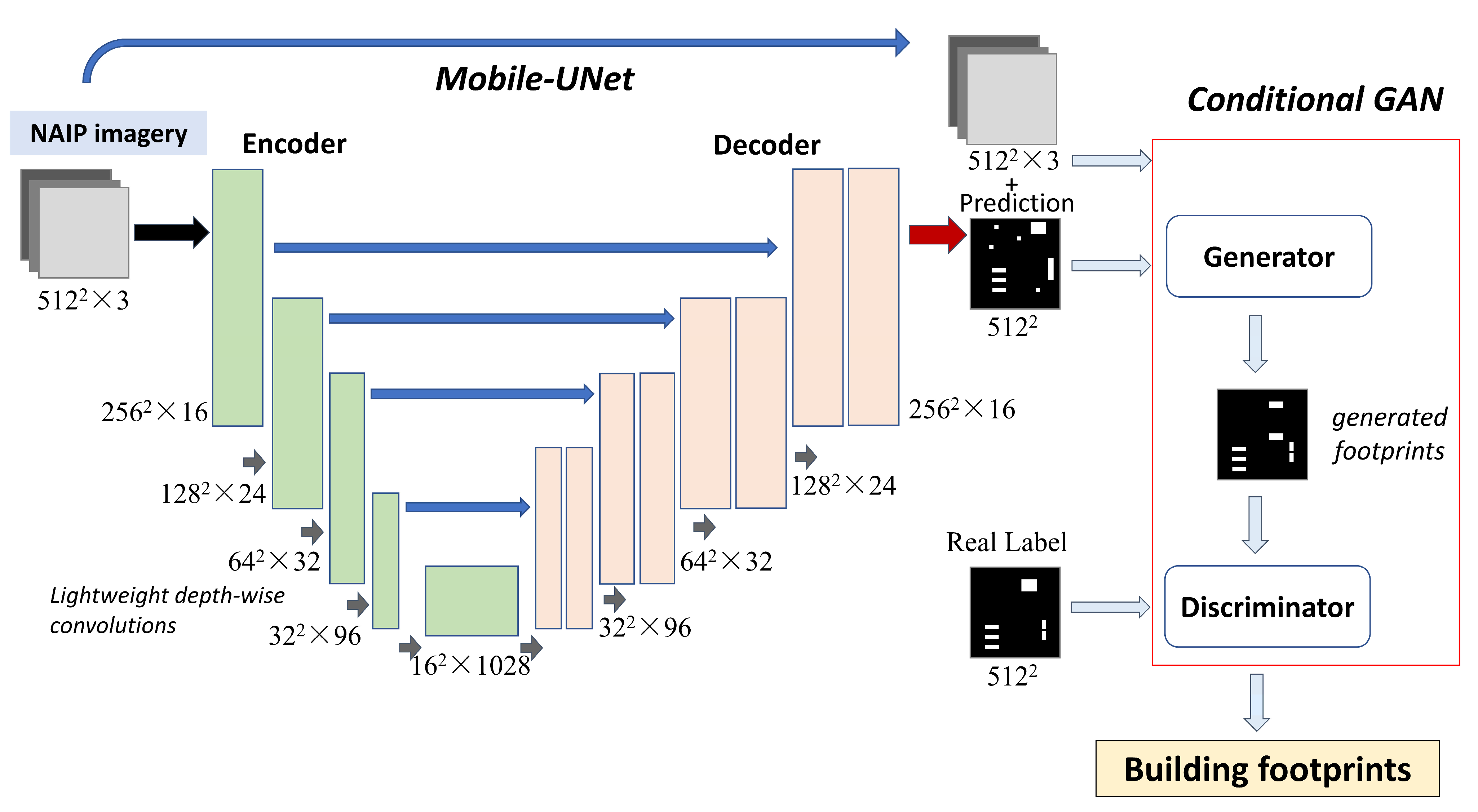
As an advanced technique in computer vision, deep learning models have recently been applied to remote sensing imagery and achieved state-of-the-art results in both pixel- and object-level classification tasks [45,46,47,48,49]. Our model framework consists of two components (Figure 2). The Mobile-UNet was first used to generate building segment candidates from NAIP images, i.e., detecting candidate building pixels [50]. The fully convolutional network (FCN) can efficiently label pixels from high-resolution images [51]. The UNet model, for example, has been used to map objects such as tree crowns, roads, and buildings from commercial satellite images or aerial photos [52,53,54,55]. The UNet network structure uses convolutional layers to perform the semantic segmentation via spatial feature extraction by encoder followed by segmentation construction by decoder [52]. A UNet-based architecture was found to perform better for buildings in WUI regions than other network structures such as FCN or DeepLabv3 [45]. We used the Mobile-UNet model due to its improved accuracy and efficiency [50]. It replaces the UNet encoder with the MobileNetV2, a simple but efficient network, for robust feature extraction [56]. The adoption of depth-wise separable convolution reduces both the size and the complexity cost of the network [56]. Moreover, its implementation requires less parameters and thus potentially minimizes the over-fitting issue [50]. Features extracted from MobileNetV2 were further deconvoluted to generate segmentation masks [50].
To refine the building segments from the Mobile-UNet, the conditional generative adversarial network (cGAN) was applied to combine the candidate map with the original input images for final prediction labels [57]. This second step is necessary due to the potential challenges of using coarser resolution imagery for building segmentation in the diverse WUI landscapes, e.g., missing pixels or partially occluded objects, and false alarms. Originally proposed as the generative model for unsupervised learning, the GAN model includes a pair of two competing networks, namely, the generator and the discriminator [57,58]. The objective of the generative network is to generate fake samples while the discriminative network aims to evaluate outputs from the generator and distinguish these generated samples from the true data distribution [58]. cGAN extends the basic GAN model to condition on external information and thus can be used for image-to-image translation [59,60]. We here adopted the model structure proposed by Isola et al. (2018), which uses a U-Net-based generator and a convolutional PatchGAN discriminator, for image translation (Figure 2). In cGAN, the generator not only aims to synthesize realistic-looking images to fool the discriminator, but also uses auxiliary information to generate images matching the labels [61]. The PatchGAN discriminator runs convolutionally across the image, focuses on each N×N patch of the image, and determines if it is real or fake [60,62]. It only penalizes the structure at the scale of image patches and then averages out all responses to make the final decision [63].

2.3. Model Implementation

2.3.1. Data Preparation

For the model development, we used the 2016 NAIP imagery for Napa and San Luis Obispo, and 2018 imagery for Shasta County to match the report years of the corresponding building footprint reference data. NAIP images were resampled from 0.6 m to 1 m, in order to apply the pre-trained model to 1 m NAIP images prior to 2016. Both the NAIP images and the reference building data were partitioned into blocks of 512 m by 512 m. We compiled a total of 2573 NAIP image subsets to cover different types of human settlement patterns in WUI, rural, and urban areas (Figure 1). These subsets represented over 10,000 buildings across these three counties. We further randomly sampled 1200 image blocks for model training and 670 blocks for the general model accuracy evaluation (Figure 1). To further examine the model performance across the four different residential patterns, the rest of 703 blocks were reserved as an independent evaluation dataset, including 128 interface WUI subsets (6573 buildings), 179 intermix WUI subsets (2430 buildings), 68 urban subsets (4878 buildings), and 327 rural subsets (1121 buildings).
To further evaluate the model’s ability in capturing both spatial and temporal dynamics of the building footprint and WUIs, we used all NAIP images from 2010 to 2018 in Lake County, and in 2010 and 2018 for Sonoma County and Orange County.

2.3.2. Model Configurations

The structure of our framework integrating two models is shown in Figure 2. The model takes image blocks at the size of 512 by 512, corresponding to 512 m by 512 m on the ground. We first applied two image preprocessing steps, histogram normalization through adaptive equalization and wavelet-based image denoising [64]. During the preliminary experiment, we also compared different input channels, including all four input bands, natural color composite (red, green, and blue), color infrared (near infrared, red, and green), and top three principal components. Simple RGB input was found to provide the best results and thus was used for this study.
The Mobile-UNet component consists of a contraction path and an expansion path. The contraction section applies an encoder with five inverted residual blocks to the input NAIP image to extract features. Each block includes the 1 × 1 convolution with the batch normalization, the rectified linear unit (ReLU) activation function, and a stride of 1; the 3 × 3 depth-wise convolution with batch-normalization, the ReLU function, and a stride of 2, and one more 1 × 1 convolution with the batch-normalization but without a non-linear function. The expansion path uses the decoder to create segmentation maps of candidate building footprints. Each upsampling layer in the decoder of the expansion section is fused with the same scale as it is in its symmetric downsampling layer.
Both the raw NAIP image and the candidate maps of building footprints were then fed into the cGAN component of the model. The generator of the cGAN follows a basic U-Net structure. The downsampler of the generator has seven 4 × 4 convolutions with the batch normalization, the LeakyReLU activation function, and a stride of 2. The upsampler uses the 4 × 4 deconvolution with the 50% dropout rate, the batch normalization, the ReLU function, and a stride of 2. The loss of the generator is calculated as the combination of the sigmoid cross entropy loss and mean absolute error between the generated image and the real image [60]. The PatchGAN discriminator applies blocks of 4 × 4 convolutions with batch normalization and LeakyReLU activation to generate 30 × 30 patches. It uses the Adam optimizer to minimize the sum of the sigmoid cross entropy losses of the real and the generated images.
The resulting images of building segmentations were further converted into shapefile format for geospatial analysis and applications. Finally, we applied a post-processing algorithm to smooth the output building segmentations, remove noise pixels, and regularize the shape and the geometry [65,66,67]. Specifically, we cleaned small polygons smaller than 4 m2 and straightened narrow sides of any building outline shorter than 4 m.

2.4. Model Evaluation

We evaluated the model performance at the building segment level with testing and evaluation datasets, respectively. Evaluations were performed at the county level and across four types of residential landscape, i.e., urban, interface WUI, intermix WUI, and rural areas. Besides overall pixel level accuracy, three metrics, including precision, recall, and F1 score (also known as dice score), were calculated to assess the segmentation results at the object level, according to the number of objects correctly or falsely predicted by the model, as shown by Equations (1)–(3) [68,69,70]. Precision is used to represent, out of all the detected building footprints, what percentage is truly positive, while the “recall” metrics quantifies, out of all the reference building footprints, what percentage is detected. The F1 metric provides a solid evaluation of model performance, by taking the harmonic mean of both false positives and false negatives.
P r e c i s i o n = T r u e   P o s i t i v e T r u e   P o s i t i v e + F a l s e   P o s i t i v e
R e c a l l = T r u e   P o s i t i v e T r u e   P o s i t i v e + F a l s e   N e g a t i v e
F 1 = T r u e   P o s i t i v e T r u e   P o s i t i v e + 0.5 F a l s e   P o s i t i v e + F a l s e   N e g a t i v e  
In addition, intersection of union (IoU), also known as Jaccard index, was calculated to assess the overlapping of the predicted segmentations (Equation (4)).
I o U = A r e a   o f   O v e r l a p A r e a   o f   U n i o n
Using our pre-trained model, we also detected the building footprints for another three counties, i.e., Lake, Sonoma, and Orange Counties from NAIP imagery. The 2018 wall-to-wall mapping results was compared with 2018 Microsoft building footprints generated from very high-resolution Bing images. We randomly sampled 600 512 m by 512 m sites from the WUIs of these three counties and calculated evaluation metrics. We also evaluated the spatial consistence between our whole county maps and Microsoft data through visualizations of both subset regions and aggregated 300 m building count maps across the time.

2.5. WUI Mapping

Based on detected building footprints in Lake, Sonoma, and Orange Counties from our model, we further mapped wildland urban interface. WUI is the area containing at least one housing unit per 0.16 km2 (40 acres), following the federal register’s definition [1]. Based on the vegetation information, it can be further split into intermix WUI, where vegetation coverage is higher than 50%; and interface WUI, where vegetation coverage is lower than 50% but the land is within 2.4 km to a continuously heavily vegetated area that includes 75% wildland vegetation and is larger than 5 km2 [1,3]. Additionally, if the intermix WUI is within a heavily vegetated area, it is further defined as a heavily vegetated intermix WUI [1].
We built a 30 m binary mask for vegetation and another mask for continuously heavily vegetated areas using National Land Cover Data (NLCD) available in 2011, 2013, 2016, and 2019 [71]. Forests, shrublands, herbaceous plants, and woody wetlands from the NLCD layers are masked as the vegetation. We then applied the moving window approach to quantify the housing density, the vegetation cover, and the distance to remote areas. The 400 m by 400 m moving window size (16 ha, 40 acres) was chosen to calculate housing density. For each 30 m pixel, if a housing unit exists in the 16 ha moving window, the vegetation percentage is then examined within the neighborhood of the pixel. If the fractional vegetation cover is higher than 50%, the pixel is labeled as the intermix WUI. However, if the vegetation cover is lower than 50% but the closest continuously heavily vegetated zone of the pixel is within 2.4 km, the pixel is labeled as the interface WUI. For an intermix WUI pixel, if the vegetation coverage is higher than 75% within the 2.25 km by 2.25 km moving window (5 km2), the pixel is further classified as highly vegetated intermix WUI.
To evaluate the model applicability in county-wide WUI mapping, we generated WUI maps for the Lake, Sonoma, and Orange Counties in 2010, based on the building footprints detected in this study. Results of the 2010 WUI mapping were compared with the existing widely used WUI maps, developed by SILVIS lab [7]. The SILVIS WUI map relied on the housing density data from TIGER at the census block scale, available in 1990, 2000, and 2010 [3]. We also derived another set of WUI maps using the Microsoft building footprints, available only in 2018, for comparison. To examine if our approach can capture the temporal dynamics of WUI areas, we further performed a wall-to-wall mapping of the WUI region in the whole Lake County for the year of 2010, 2012, 2014, 2016, and 2018.

3. Results

3.1. Model Performance

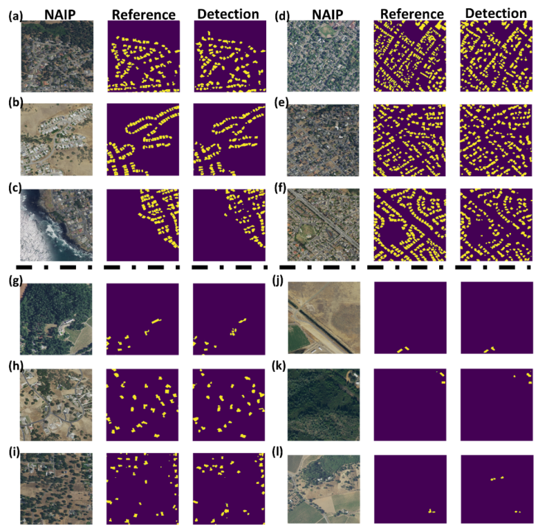
The integrative deep learning model was built with the 1200 NAIP image blocks, using the labeled reference data in three counties. Overall, it performed well in detecting building footprints over California’s diverse landscape with various housing density (Figure 3). A visual inspection of examples over the independent evaluation blocks showed that the majority of the reference buildings were identified correctly over the interface WUI (Figure 3a–c) and urban areas (Figure 3d–f), and the mapped building footprints aligned well with reference buildings. For example, houses within Cambria Pines near Moonstone Park (Figure 3a) and the community next to barren areas around Lake Nacimiento (Figure 3b) were all been detected. The model also showed a good performance over areas where buildings intermingled with vegetation (Figure 3g–i) and where few buildings scattered across the landscape dominated by forests or bare soil (Figure 3h,i). Our approach even identified buildings omitted by the reference data in the rural areas of Calistoga (Figure 3l). Occasionally several adjacent buildings were identified as one large building segment, for example in dense urban areas, and the size of some detected building segmentations were smaller than that of the reference, such as the pixel-level omission at the building edges (Figure 3d,f).
A comparison with the full testing dataset from 670 blocks showed a high overall pixel level accuracy of 97% for building segmentation (Table 1). An F1 score of 0.53 and IoU of 0.52 suggest a reasonable performance on the individual building detection. Similar results were found when evaluated with the additional evaluation dataset with an F1 score of 0.64 and IoU of 0.5. The accuracy of our approach varied slightly with housing density (Table 2). Relatively more precise and robust results were found over less populated regions such as intermix WUI or rural areas, as shown by F1 scores of 0.67 for the intermix WUI and 0.75 for rural regions vs. 0.62 for interface and urban areas, and higher percentages of predicted building objects being correctly mapped in dense residential areas. However, relatively lower recall values for these two sparse regions, especially for the intermix WUI, indicated potential omission of some buildings when they are highly intermixed with vegetation. In interface WUI, the model captured the individual buildings slightly better than in the intermix WUI and rural areas. We also found larger overlapping between the NAIP-based building segmentation and the reference building footprints in the interface WUI and urban areas (IoU of 0.53) vs. 0.47 for intermix and 0.43 for rural areas. Similarly, better results were found in counties with more dispersed building patterns, i.e., San Luis Obispo and Shasta Counties, than counties with more dense communities such as Napa County, as shown by much higher F1 scores and IoU across the four different types of human settlements.
The model also captured the total building count and footprint coverage well along the gradient of different housing densities across multiple counties (Table 2). The result showed a very good agreement on the percentage of identified building footprint areas, with an error of around 1% in dense settlements compared with the ground truth information. It detected 80% of the building count in the interface areas, accounting for 5.1% of the total land area, similar to 6.15% from the reference data. In the intermix region, the model slightly overestimated the total building count but mapped a similar total percentage of the building area (1.39% vs. 1.47%). The detected building footprint areas in regions with very dense or sparse housing also agreed well with the reference data, accounting for (7.26% vs. 8.83%) and (0.39% vs. 0.40%) of the land areas, respectively.
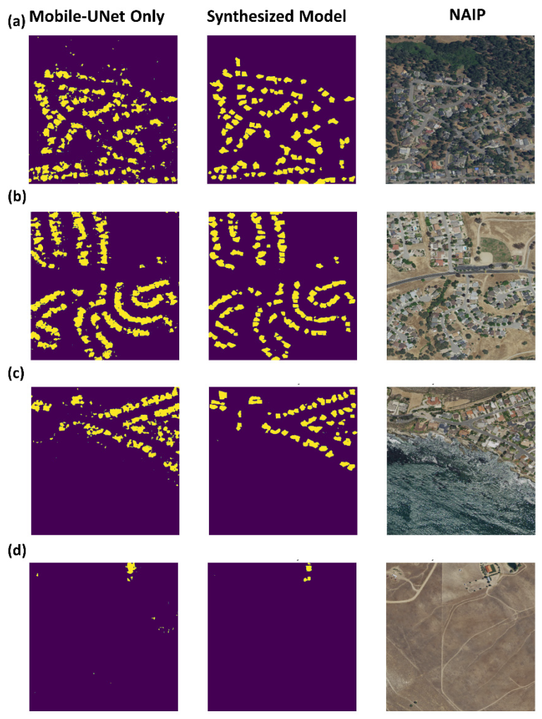
The integrative model developed here significantly improved the accuracy of building footprint detection, compared with Mobile-UNet only and cGAN only models (Table 1). It had a more balanced performance, as shown by the higher F1 score of 0.53 in the testing dataset and 0.64 in the evaluation dataset, compared with 0.41 and 0.48 by Mobile-UNet, as well as 0.31 and 0.35 by cGAN only. Although the Mobile-UNet model itself identified a higher percentage of reference building objects (recall), it caused false detection more likely as indicated by its lower precision (Table 1 and Figure 4). For example, some discrete and noisy pixels falsely detected by Mobile-UNet over intermix WUI or rural areas, probably due to the confusion with bare ground, were removed by applying the cGAN to the Mobile-UNet results and NAIP images at a second step (Figure 4b,c). Incorporation of cGAN also improved separating the adjacent buildings and filled the missing pixels for relatively large buildings in the Mobile-UNet outputs (Figure 4a,b). For example, predictions of Mobile-UNet clumped adjacent buildings together as one large and long object in communities by the Moonstone beach in Cambria and the buildings close to the Nacimiento Lake in Paso Robles (Figure 4a,b). The synthesized model, however, successfully solved this problem by learning the separation of those mixed pixels with building boundaries and residential spacings in input images.

3.2. Building Footprint Mapping and Patterns

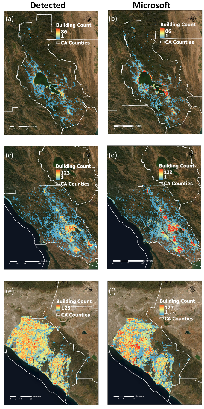
We applied the trained model to the time series of NAIP imagery and mapped individual building footprints for Lake, Sonoma, and Orange Counties every 2 years from 2010 to 2018. For county-wide visualization purposes, we aggregated the building footprints into building count at 300 m resolution (Figure 5 and Figure 6). The building footprint mapping based on our approach captured the human settlement patterns from more remote to suburban counties well (Figure 5). For example, in Lake County, areas such as Clearlake city and Lakeport city were well-identified as dense residential clusters and the expansion of the houses to the WUI region was also delineated (Figure 5a). Orange County was mapped as highly urbanized, with few smaller communities such as Silverado scattered in the rural region (Figure 5e). In Sonoma County, on the other hand, most buildings were clustered around Santa Rosa and human settlements spread towards the wildland areas (Figure 5c). Overall, the building patterns from our approach matched the 2018 Microsoft data, as shown by the building density aggregated at 300 m (Figure 5b,d,f). However, missing buildings from our detection may exist in the very dense region. Across the random samples from each county, our detected building footprints showed good consistency with Microsoft data, with F1 scores over 0.6 for all three counties. For Lake and Sonoma counties with sparse housing arrangements, our predictions have high precision scores of 0.79 and 0.83, but relatively low recalls of 0.62 and 0.47 as reference to Microsoft buildings. Conversely, in Orange County with dense interface WUIs or cities, the predictions have a lower precision of 0.54 but a recall of 0.79, possibly constrained by the limited number of urban trainings sampled in the model.
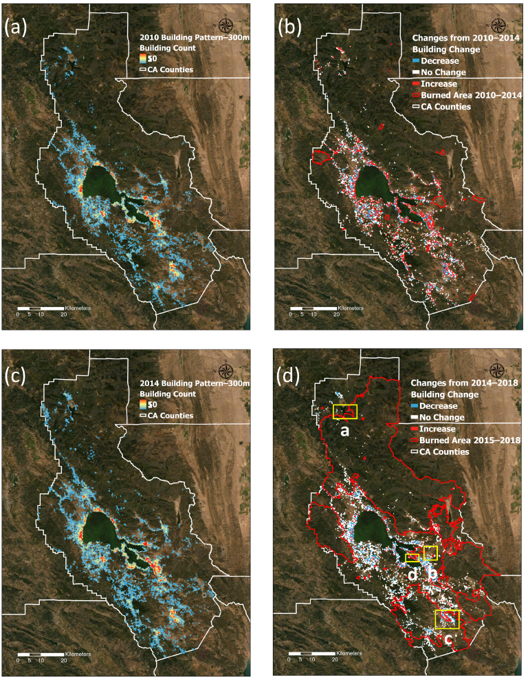
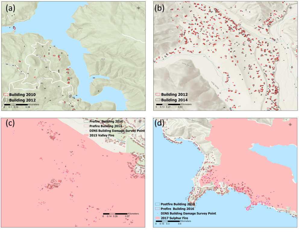
The time series of building footprints derived from NAIP imagery captured the dynamics of building expansion, for example, in Lake County (Figure 6). The total number of houses increased from 34,566 in 2010 to 45,695 in 2014 (Figure 6a,b). Transitions from rural to human settlements, such as infills, community expansion, and new community development were well-captured by the model. The intermix WUI region showed an increase in both building density, e.g., around the town of Clear Lake, and area expansion, e.g., new residential communities in the southern and northeastern parts of the county. Example subsets were shown at the individual building level (Figure 7). Our approach detected recreational houses built between 2010 and 2012 around Lake Pillsbury, as well as the changes in structures such as the dam across the Eel River and piers along the shoreline of the lake (Figure 7a). New houses were also detected across the whole Spring Valley community and along the Spring Valley Road and Long Valley Road in the southwest of the community, resulting in increased housing density by approximately 25% from 2012 to 2014 in the local community (Figure 7b).
Our approach also identified building reduction caused by wildfire events. We found that the number of mapped buildings decreased by around 20% in 2018 from 2014. A closer examination of Lake County’s fire history showed that around 2000 km2, approximately 57% of the total area in Lake County, were burned during 2015–2018 (Figure 6d), especially over the eastern and southern parts of the county, covering southern Mendocino National Forests and Cache Creek Wilderness. We found that a total of 6,768 buildings shown in the 2014 building footprint map (Figure 6c) were within the 2015–2018 fire perimeters and 2459 buildings were destroyed. This result was consistent with the DINS building survey which recorded a total of 2982 buildings damaged by 2015–2018 fire events in Lake County.
Although not designed for mapping building damage, the approach from this study captured the building loss from wildfires well (Figure 7c,d). For example, over the 30,790 ha burned by the 2015 Valley fire, we found 2078 buildings, out of 3574 buildings in our pre-fire building footprint map, disappeared in our postfire building footprint map (Figure 7c), while 80 out of 165 buildings were destroyed over the 892.8 ha burned by 2017 Sulphur fire (Figure 7d). The numbers and locations of building loss were consistent with those from the DINS postfire building damage survey.

3.3. WUI Mapping—Spatial Patterns and Temporal Dynamics

We generated WUI maps every two years since 2010 in three counties, i.e., Lake, Sonoma, and Orange, using the building footprints derived from NAIP 1 m imagery with our approach and the NLCD vegetation map [72]. Overall, our WUI maps showed similar spatial patterns with the existing 2010 census tract-based SILVIS WUI maps within each county and across counties (Figure 8). For example, in Lake County, both approaches identified major clusters of interface WUI around the boundaries of major cities, such as Lakeport, Kelseyville, and Clearlake, around Lake Clear, transitioning into intermix WUI and highly vegetated regions. In the more urbanized counties (Figure 8d–i), such as Orange and Sonoma, our approach successfully mapped those WUI areas with a low housing density, especially those large census tracts with small housing clusters scattered within vegetated wildlands, which further captured the spatial spanning of the WUI clusters. Orange County has the largest WUI interface areas, followed by Sonoma, and Lake Counties. In contrast, Sonoma and Lake Counties have much larger intermixed WUI areas, similar to what were shown by SILVIS maps.
However, our 30 m WUI maps identified larger WUI areas and showed more granularity and smoother transition from urban to WUI areas than SILVIS maps. Overall, the results from this study were similar to patterns derived from the Microsoft building footprints (Figure 8c,f,i). In Lake County, our approach mapped a total WUI area of 468 km2, dominated by intermix WUI (375 vs. 94 km2 of interface WUI), compared with 411 km2 from the SILVIS WUI map (334 km2 of intermix WUI vs. 78 km2 of interface WUI). Our results identified total WUI areas of 1635 km2 in Sonoma County and 660 km2 in Orange County, which were 28% higher than, and almost doubled the SILVIS estimates, respectively. Among the WUI areas, both our maps and SILVIS maps showed that the intermix WUI was dominant in Sonoma County, accounting for 74% and 77% of the WUI areas; while Orange County was dominated by interface WUI, contributing to 80% based on our map and 82% in the SILVIS WUI map.
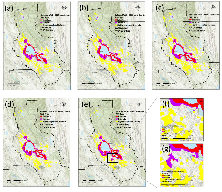
Using bi-annual building density and vegetation maps, the approach developed in this study captured well the temporal dynamics of WUI areas and types. For example, the time series of derived WUI maps in Lake County showed the changes in WUI regions every 2 years from 2010 to 2018 (Figure 9), associated with urban sprawl and wildfire disasters. We found that the combined area of interface and intermix WUI fluctuated from year to year. In the first half of the 2010s, WUI areas expanded steadily, reaching 210 km2 in 2012 and 215.6 km2 in 2014. The majority of expansions was found in the regions transitioning from wildlands to intermix WUI regions, with additional housing development in some tracts of highly vegetated intermix regions further away from populated towns (Figure 9f,g). After the 2015 extreme fire events, the total WUI areas decreased to 199.4 km2 in 2016, but then increased to 215.5 km2 in 2018 following the community rebuilding [73,74,75]. Our approach also detected that a continuous highly vegetated intermix region has evolved into the intermix WUI in the southwest of the county in 2018.

4. Discussion

Our study demonstrated the possibility of an efficient approach for building surveys from high resolution images and improved the temporal and spatial accuracy of WUI mapping. Further improvements are needed for operational and broader applications. First, the building detection in this study was limited by the 1 m NAIP imagery in order to take advantage of the historical archives for bi-annual mapping. An improvement of the model can be based on the 0.6 m NAIP images in California after 2016 to better resolve the mixed pixel issues at the edge of the buildings. Additionally, some uncertainties in our building detection may be caused by some inconsistency in NAIP image acquisitions, such as varying viewing angles, sunlight conditions, and imaging days across different images. Although denoising and equalization during preprocessing can help harmonize differences in ground reflection, calibration of the input images across the space and time can further improve the accuracy and generalization of the model. Whenever possible, other well-calibrated high-resolution imagery can also be used as additional sources for improved local scale mapping. Secondly, improved accuracy of ground truth building footprints data are also needed, especially in intermix and rural areas.
Moreover, the building detection model in this study was trained mostly on images within the WUI regions due to the WUI focus of our study. Although when applied into a large region, the model can successfully capture the spatial extent of housing development areas, regions such as urban or dense residential areas might be less represented. Lastly, in this study, we used Mobile-UNet as the backbone of the model architecture considering its efficiency in applications. A previous study on WUI building detection showed that the UNet-based structure has promising performance; however, a more sophisticated feature extractor, such as ResNet or VGG models, can better optimize the model performance and improve detection accuracy through considerably increased network depth [76,77].
The improved performance of the combined network structure by stacking UNet or GAN was consistent with previous studies for image harmonization and noise cleaning for products derived from medical or remote sensing images [78,79,80,81]. Through image-to-image translation, GAN can serve as a post-processing process to reinforce spatial contiguity, remove artifacts or undesired objects, and boost and harmonize the quality of predictions from relatively low-resolution or compressed inputs [80,81]. Only a limited number of studies have focused on building detection in WUI at 1 m resolution. Caggiano et al. detected building footprints within sparse WUIs using object-based approaches in four counties of Colorado from NAIP images in 2014 [82,83]. Their approach achieved an overall accuracy fluctuated from 50 to 95%, a precision of 0.66, and recall of 0.51 [82]. The other study in WUI achieved a high F1 score of around 0.8, but was based on 0.5 m fused commercial SuperView-1 satellite data, which has twice as high resolution as NAIP images [45].
Most previous research of building detection have focused on urban regions, which had quite different landscapes and housing patterns from wildland urban interfaces. Although trained for the WUI areas, our model had a decent performance, F1 of 0.61, and IoU of 0.53, over the urban regions. Compared with urban building segmentation models, our model had very competitive recall scores, but slightly lower precision scores, possibly due to the much fewer urban samples in our training data [37]. For instance, Locally Constrained You-Only-Look-Once (YOLO) framework for object detection was developed for NAIP images with F1 scores varying from 0.73 to 0.8 across testing cities in Minnesota [36]. For similar studies using semantic building segmentation methods on NAIP images within urban regions, deep learning models such as segNet, CRFasRNN, or FCN were constructed for dense residential areas in the U.S. and achieved the overall accuracy ranging from 0.62 to 0.71 and IoU ranging from 0.45 to 0.58 [37,84]. As shown in these studies, the model built on dense urban regions performed relatively worse with high false positives when applied to sparse landscapes such as desert, mountainous areas, or agricultural lands, and requires further modification and retraining of the model [37,84].
In terms of WUI mapping, our approach improved upon previous methods and is able to delineate the natural transition from dense urban regions to WUIs and rural human settlements. Currently, the most widely used SILVIS WUI dataset relied on housing densities from census tract regions, which captures spatial heterogeneity at relatively coarse scales [7]. Although there were several other recent studies exploring the possibilities of using building locations or individual building information for WUI mapping, these results were only available for 1 static year while our bi-annual WUI maps provide more frequent updates with free NAIP imagery [31,85].

5. Conclusions

We developed and evaluated a deep learning framework to detect individual building footprints over the transitional areas from urban to wildland in this study. By taking advantage of the publicly available NAIP aerial imagery at meter scale, our framework provides an efficient approach to provide high resolution building footprint maps every other year. Our analysis in California showed that the combination of Mobile-UNet and generative adversarial network had a more balanced detection performance. When examined at a large scale over three counties, the total building area agreed well with that derived from the reference building area. Bi-annual footprint maps of Lake, Sonoma, and Orange Counties showed the capability of the integrated approach to capture the spatial patterns and dynamics associated with urban expansion and wildfire damages. We further applied a moving window-based workflow for WUI mapping using the derived fine scale building footprints. The resulting WUI maps showed finer granularity than those from census tract-based housing density, and are expected to contribute to community development planning, wildfire risk assessment, and adaptive strategies on climate adaptation and disaster response.

Author Contributions

Conceptualization, Y.H. and Y.J.; methodology, Y.H. and Y.J.; software, Y.H.; validation, Y.H; formal analysis, Y.H.; writing, Y.H. and Y.J.; visualization, Y.H.; project administration, Y.J.; funding acquisition, Y.J. All authors have read and agreed to the published version of the manuscript.

Funding

This research was funded by NASA Land Cover and Land Use Change Program (grand # 80NSSC21K0295) and the California Strategic Growth Council under the Innovation Center for Advancing Ecosystem Climate Solutions. Partial support was also provided by the USGS’s AmericaView grant to CaliforniaView (grand # AV18-CA-01).

Data Availability Statement

Not applicable.

Acknowledgments

The authors would like to thank VeriDaas Corporation for providing the Geiger-mode LiDAR data that made this study possible; with special thanks to Stephen Griffith, for valuable discussions and feedback. In addition, we thank the Academic Editor and three anonymous reviewers for providing helpful comments and suggestions which substantially improved the manuscript.

Conflicts of Interest

The authors declare no conflict of interest. The funders had no role in the design of the study; in the collection, analyses, or interpretation of data; in the writing of the manuscript, or in the decision to publish the results.

References

  1. Glickman, D.; Babbitt, B. Urban wildland interface communities within the vicinity of federal lands that are at high risk from wildfire. Fed. Regist. 2001, 66, 751–777. [Google Scholar]
  2. Manzello, S.L.; Almand, K.; Guillaume, E.; Vallerent, S.; Hameury, S.; Hakkarainen, T. FORUM Position Paper1 The Growing Global Wildland Urban Interface (WUI) Fire Dilemma: Priority Needs for Research. Fire Saf. J. 2018, 100. [Google Scholar] [CrossRef]
  3. Radeloff, V.C.; Hammer, R.B.; Stewart, S.I.; Fried, J.S.; Holcomb, S.S.; McKeefry, J.F. The wildland–urban interface in the united states. Ecol. Appl. 2005, 15, 799–805. [Google Scholar] [CrossRef] [Green Version]
  4. Godoy, M.M.; Martinuzzi, S.; Kramer, H.A.; Defossé, G.E.; Argañaraz, J.; Radeloff, V.C. Rapid WUI growth in a natural amenity-rich region in central-western Patagonia, Argentina. Int. J. Wildland Fire 2019, 28, 473. [Google Scholar] [CrossRef]
  5. Johnson, K.; Nucci, A.; Long, L. Population trends in metropolitan and nonmetropolitan America: Selective deconcentration and the rural rebound. Popul. Res. Policy Rev. 2005, 24, 527–542. [Google Scholar] [CrossRef]
  6. Martinuzzi, S.; Stewart, S.I.; Helmers, D.P.; Mockrin, M.H.; Hammer, R.B.; Radeloff, V.C. The 2010 Wildland-Urban Interface of the Conterminous United States; Research Map NRS-8; US Department of Agriculture, Forest Service, Northern Research Station: Newtown Square, PA, USA, 2018; 124p, Available online: https://www.fs.fed.us/nrs/pubs/rmap/rmap_nrs8.pdf (accessed on 15 April 2022).
  7. Radeloff, V.C.; Helmers, D.P.; Kramer, H.A.; Mockrin, M.H.; Alexandre, P.M.; Bar-Massada, A.; Butsic, V.; Hawbaker, T.J.; Martinuzzi, S.; Syphard, A.D.; et al. Rapid growth of the US wildland-urban interface raises wildfire risk. Proc. Natl. Acad. Sci. USA 2018, 115, 3314–3319. [Google Scholar] [CrossRef] [PubMed] [Green Version]
  8. Faivre, N.; Jin, Y.; Goulden, M.L.; Randerson, J.T. Controls on the spatial pattern of wildfire ignitions in Southern California. Int. J. Wildland Fire 2014, 23, 799–811. [Google Scholar] [CrossRef] [Green Version]
  9. Haynes, K.; Short, K.; Xanthopoulos, G.; Viegas, D.; Ribeiro, L.M.; Blanchi, R. Wildfires and WUI fire fatalities. In Encyclopedia of Wildfires and Wildland-Urban Interface (WUI) Fires; Manzello, S.L., Ed.; Springer: Cham, Switzerland, 2020; p. 16. [Google Scholar]
  10. Schulze, S.S.; Fischer, E.C.; Hamideh, S.; Mahmoud, H. Wildfire impacts on schools and hospitals following the 2018 California Camp Fire. Nat. Hazards 2020, 104, 901–925. [Google Scholar] [CrossRef]
  11. Bar-Massada, A.; Stewart, S.I.; Hammer, R.B.; Mockrin, M.H.; Radeloff, V.C. Using structure locations as a basis for mapping the wildland urban interface. J. Environ. Manag. 2013, 128, 540–547. [Google Scholar] [CrossRef]
  12. Johnston, L.M.; Flannigan, M.D. Mapping Canadian wildland fire interface areas. Int. J. Wildland Fire 2017, 27, 1–14. [Google Scholar] [CrossRef]
  13. Nguyen, M.H.; Block, J.; Crawl, D.; Siu, V.; Bhatnagar, A.; Rodriguez, F.; Kwan, A.; Baru, N.; Altintas, I. Land cover classification at the wildland urban interface using high-resolution satellite imagery and deep learning. In Proceedings of the 2018 IEEE International Conference on Big Data (Big Data), Seattle, WA, USA, 10–13 December 2018; pp. 1632–1638. [Google Scholar] [CrossRef]
  14. Miranda, A.; Carrasco, J.; González, M.; Pais, C.; Lara, A.; Altamirano, A.; Weintraub, A.; Syphard, A.D. Evidence-based mapping of the wildland-urban interface to better identify human communities threatened by wildfires. Environ. Res. Lett. 2020, 15, 094069. [Google Scholar] [CrossRef]
  15. Stewart, S.I.; Radeloff, V.C.; Hammer, R.B.; Hawbaker, T.J. Defining the wildland–urban interface. J. For. 2007, 105, 201–207. [Google Scholar]
  16. U.S. Census Bureau. Available online: https://www2.census.gov/geo/tiger/TIGER2021/TRACT/ (accessed on 6 May 2022).
  17. Conedera, M.; Tonini, M.; Oleggini, L.; Orozco, C.V.; Leuenberger, M.; Pezzatti, G.B. Geospatial approach for defining the Wildland-Urban Interface in the Alpine environment. Comput. Environ. Urban Syst. 2015, 52, 10–20. [Google Scholar] [CrossRef]
  18. Zhong, Y.; Fei, F.; Liu, Y.; Zhao, B.; Jiao, H.; Zhang, L. SatCNN: Satellite image dataset classification using agile convolutional neural networks. Remote Sens. Lett. 2016, 8, 136–145. [Google Scholar] [CrossRef]
  19. Chen, Y.; Ming, D.; Lv, X. Superpixel based land cover classification of VHR satellite image combining multi-scale CNN and scale parameter estimation. Earth Sci. Inform. 2019, 12, 341–363. [Google Scholar] [CrossRef]
  20. Bischke, B.; Helber, P.; Folz, J.; Borth, D.; Dengel, A. Multi-Task Learning for Segmentation of Building Footprints with Deep Neural Networks. In Proceedings of the 2019 IEEE International Conference on Image Processing (ICIP), Taipei, Taiwan, 22–25 September 2019; pp. 1480–1484. [Google Scholar] [CrossRef] [Green Version]
  21. Rastogi, K.; Bodani, P.; Sharma, S.A. Automatic building footprint extraction from very high-resolution imagery using deep learning techniques. Geocarto Int. 2020, 37, 1501–1513. [Google Scholar] [CrossRef]
  22. Guo, H.; Su, X.; Tang, S.; Du, B.; Zhang, L. Scale-Robust Deep-Supervision Network for Mapping Building Footprints From High-Resolution Remote Sensing Images. IEEE J. Sel. Top. Appl. Earth Obs. Remote Sens. 2021, 14, 10091–10100. [Google Scholar] [CrossRef]
  23. Touzani, S.; Granderson, J. Open Data and Deep Semantic Segmentation for Automated Extraction of Building Footprints. Remote Sens. 2021, 13, 2578. [Google Scholar] [CrossRef]
  24. Ekim, B.; Sertel, E. A Multi-Task Deep Learning Framework for Building Footprint Segmentation. In Proceedings of the 2021 IEEE International Geoscience and Remote Sensing Symposium IGARSS, Brussels, Belgium, 11–16 July 2021; pp. 2500–2503. [Google Scholar]
  25. Liu, T.; Yang, L. A Fully Automatic Method for Rapidly Mapping Impacted Area by Natural Disaster. In Proceedings of the InIGARSS 2020—2020 IEEE International Geoscience and Remote Sensing Symposium, Waikoloa, HI, USA, 26 September–2 October 2020; pp. 6906–6909. [Google Scholar]
  26. Liu, T.; Yang, L.; Lunga, D. Change detection using deep learning approach with object-based image analysis. Remote Sens. Environ. 2021, 256, 112308. [Google Scholar] [CrossRef]
  27. Pepe, M.; Costantino, D.; Alfio, V.S.; Vozza, G.; Cartellino, E. A Novel Method Based on Deep Learning, GIS and Geomatics Software for Building a 3D City Model from VHR Satellite Stereo Imagery. ISPRS Int. J. Geo-Inf. 2021, 10, 697. [Google Scholar] [CrossRef]
  28. Buyukdemircioglu, M.; Kocaman, S.; Kada, M. DEEP LEARNING FOR 3D BUILDING RECONSTRUCTION: A REVIEW. ISPRS Int. Arch. Photogramm. Remote Sens. Spat. Inf. Sci. 2022, XLIII-B2-2, 359–366. [Google Scholar] [CrossRef]
  29. Microsoft U.S. Building Footprints. 2018. Available online: https://github.com/microsoft/USBuildingFootprints (accessed on 4 October 2021).
  30. Hou, D.; Miao, Z.; Xing, H.; Wu, H. Two novel benchmark datasets from ArcGIS and bing world imagery for remote sensing image retrieval. Int. J. Remote Sens. 2020, 42, 240–258. [Google Scholar] [CrossRef]
  31. Li, S.; Dao, V.; Kumar, M.; Nguyen, P.; Banerjee, T. Mapping the wildland-urban interface in California using remote sensing data. Sci. Rep. 2022, 12, 1–12. [Google Scholar] [CrossRef] [PubMed]
  32. Su, J.; Vargas, D.V.; Sakurai, K. One Pixel Attack for Fooling Deep Neural Networks. IEEE Trans. Evol. Comput. 2019, 23, 828–841. [Google Scholar] [CrossRef] [Green Version]
  33. Dechesne, C.; Lassalle, P.; Lefèvre, S. Bayesian U-Net: Estimating Uncertainty in Semantic Segmentation of Earth Observation Images. Remote Sens. 2021, 13, 3836. [Google Scholar] [CrossRef]
  34. NAIP Information Sheet. 2015. Available online: https://www.fsa.usda.gov/Internet/FSA_File/naip_info_sheet_2015.pdf (accessed on 10 November 2021).
  35. Cleve, C.; Kelly, M.; Kearns, F.R.; Moritz, M. Classification of the wildland–urban interface: A comparison of pixel- and object-based classifications using high-resolution aerial photography. Comput. Environ. Urban Syst. 2008, 32, 317–326. [Google Scholar] [CrossRef]
  36. Xie, Y.; Cai, J.; Bhojwani, R.; Shekhar, S.; Knight, J. A locally-constrained YOLO framework for detecting small and densely-distributed building footprints. Int. J. Geogr. Inf. Sci. 2020, 34, 777–801. [Google Scholar] [CrossRef]
  37. Yang, H.L.; Yuan, J.; Lunga, D.; Laverdiere, M.; Rose, A.; Bhaduri, B. Building Extraction at Scale Using Convolutional Neural Network: Mapping of the United States. IEEE J. Sel. Top. Appl. Earth Obs. Remote Sens. 2018, 11, 2600–2614. [Google Scholar] [CrossRef] [Green Version]
  38. Kusz, M.; Peters, J.; Huber, L.; Davis, J.; Michael, S. Building Detection with Deep Learning. In Proceedings of the Practice and Experience in Advanced Research Computing, Portland, OR, USA, 17 July 2021; pp. 1–8. [Google Scholar]
  39. Yu, K.; Frank, H.; Wilson, D. Points 2 Polygons: Context-Based Segmentation from Weak Labels Using Adversarial Networks. arXiv 2021, arXiv:2106.02804. [Google Scholar]
  40. Theobald, D.M.; Romme, W.H. Expansion of the US wildland–urban interface. Landsc. Urban Plan. 2007, 83, 340–354. [Google Scholar] [CrossRef]
  41. Kramer, H.A.; Mockrin, M.H.; Alexandre, P.M.; Radeloff, V.C. High wildfire damage in interface communities in California. Int. J. Wildland Fire 2019, 28, 641–650. [Google Scholar] [CrossRef] [Green Version]
  42. Napa County Building Footprints. Available online: http://gis.napa.ca.gov/giscatalog/catalog_xml.asp (accessed on 15 April 2022).
  43. Shasta County Building Footprints. Available online: https://data-shasta.opendata.arcgis.com/datasets/Shasta:buildingfootprints/about (accessed on 15 April 2022).
  44. San Luis Obispo County Building Footprints. Available online: https://opendata.slocounty.ca.gov/datasets/building-footprints/explore (accessed on 15 April 2022).
  45. Chen, D.-Y.; Peng, L.; Li, W.-C.; Wang, Y.-D. Building Extraction and Number Statistics in WUI Areas Based on UNet Structure and Ensemble Learning. Remote Sens. 2021, 13, 1172. [Google Scholar] [CrossRef]
  46. Zhu, X.X.; Tuia, D.; Mou, L.; Xia, G.S.; Zhang, L.; Xu, F.; Fraundorfer, F. Deep learning in remote sensing: A comprehensive review and list of resources. IEEE Geosci. Remote Sens. Mag. 2017, 5, 8–36. [Google Scholar] [CrossRef] [Green Version]
  47. Kussul, N.; Lavreniuk, M.; Skakun, S.; Shelestov, A. Deep Learning Classification of Land Cover and Crop Types Using Remote Sensing Data. IEEE Geosci. Remote Sens. Lett. 2017, 14, 778–782. [Google Scholar] [CrossRef]
  48. Liu, Y.; Chen, X.; Wang, Z.; Wang, Z.J.; Ward, R.K.; Wang, X. Deep learning for pixel-level image fusion: Recent advances and future prospects. Inf. Fusion 2018, 42, 158–173. [Google Scholar] [CrossRef]
  49. Yuan, Q.; Shen, H.; Li, T.; Li, Z.; Li, S.; Jiang, Y.; Xu, H.; Tan, W.; Yang, Q.; Wang, J.; et al. Deep learning in environmental remote sensing: Achievements and challenges. Remote Sens. Environ. 2020, 241, 111716. [Google Scholar] [CrossRef]
  50. Jing, J.; Wang, Z.; Rätsch, M.; Zhang, H. Mobile-Unet: An efficient convolutional neural network for fabric defect detection. Text. Res. J. 2022, 92, 30–42. [Google Scholar] [CrossRef]
  51. Xu, Y.; Wu, L.; Xie, Z.; Chen, Z. Building Extraction in Very High Resolution Remote Sensing Imagery Using Deep Learning and Guided Filters. Remote Sens. 2018, 10, 144. [Google Scholar] [CrossRef] [Green Version]
  52. Ronneberger, O.; Fischer, P.; Brox, T. U-net: Convolutional networks for biomedical image segmentation. In Proceedings of the International Conference on Medical image computing and computer-assisted intervention, Cham, Switzerland, 5 October 2015; pp. 234–241. [Google Scholar]
  53. Wagner, F.H.; Sanchez, A.; Tarabalka, Y.; Lotte, R.G.; Ferreira, M.P.; Aidar, M.P.; Gloor, E.; Phillips, O.L.; Aragao, L.E. Using the U-net convolutional network to map forest types and disturbance in the Atlantic rainforest with very high resolution images. Remote Sens. Ecol. Conserv. 2019, 5, 360–375. [Google Scholar] [CrossRef] [Green Version]
  54. Yang, X.; Li, X.; Ye, Y.; Lau, R.Y.K.; Zhang, X.; Huang, X. Road Detection and Centerline Extraction Via Deep Recurrent Convolutional Neural Network U-Net. IEEE Trans. Geosci. Remote Sens. 2019, 57, 7209–7220. [Google Scholar] [CrossRef]
  55. Ivanovsky, L.; Khryashchev, V.; Pavlov, V.; Ostrovskaya, A. Building detection on aerial images using U-NET neural networks. In Proceedings of the 2019 24th Conference of Open Innovations Association (FRUCT), Moscow, Russia, 8 April 2019; pp. 116–122. [Google Scholar]
  56. Sandler, M.; Howard, A.; Zhu, M.; Zhmoginov, A.; Chen, L.C. Mobilenetv2: Inverted residuals and linear bottlenecks. In Proceedings of the IEEE conference on computer vision and pattern recognition, Salt Lake City, UT, USA, 18–23 June 2018; pp. 4510–4520. [Google Scholar]
  57. Goodfellow, I.; Pouget-Abadie, J.; Mirza, M.; Xu, B.; Warde-Farley, D.; Ozair, S.; Courville, A.; Bengio, Y. Generative adversarial nets. Adv. Neural Inf. Processing Syst. 2014, 27, 2672–2680. [Google Scholar]
  58. Creswell, A.; White, T.; Dumoulin, V.; Arulkumaran, K.; Sengupta, B.; Bharath, A.A. Generative Adversarial Networks: An Overview. IEEE Signal Process. Mag. 2018, 35, 53–65. [Google Scholar] [CrossRef] [Green Version]
  59. Gauthier, J. Conditional generative adversarial nets for convolutional face generation. Winter Semester 2014, 2014, 2. [Google Scholar]
  60. Isola, P.; Zhu, J.Y.; Zhou, T.; Efros, A.A. Image-to-image translation with conditional adversarial networks. In Proceedings of the IEEE Conference on Computer Vision and Pattern Recognition, Honolulu, HI, USA, 21–26 July 2017; pp. 1125–1134. [Google Scholar]
  61. Mirza, M.; Osindero, S. Conditional generative adversarial nets. arXiv 2014, arXiv:1411.1784. [Google Scholar]
  62. Li, C.; Wand, M. Precomputed Real-Time Texture Synthesis with Markovian Generative Adversarial Networks. In Proceedings of the European Conference on Computer Vision, Amsterdam, The Netherlands, 11–14 October 2016; pp. 702–716. [Google Scholar] [CrossRef] [Green Version]
  63. Demir, U.; Unal, G. Patch-based image inpainting with generative adversarial networks. arXiv 2018, arXiv:1803.07422. [Google Scholar]
  64. Gorgel, P.; Sertbas, A.; Ucan, O.N. A Wavelet-Based Mammographic Image Denoising and Enhancement with Homomorphic Filtering. J. Med. Syst. 2009, 34, 993–1002. [Google Scholar] [CrossRef] [PubMed]
  65. Bayer, T. Automated Building Simplification Using a Recursive Approach. In Cartography in Central and Eastern Europe; Springer: Berlin/Heidelberg, Germany, 2009; pp. 121–146. [Google Scholar] [CrossRef] [Green Version]
  66. Yekeen, S.T.; Balogun, A.-L.; Yusof, K.B.W. A novel deep learning instance segmentation model for automated marine oil spill detection. ISPRS J. Photogramm. Remote Sens. 2020, 167, 190–200. [Google Scholar] [CrossRef]
  67. Goutte, C.; Gaussier, E. A probabilistic interpretation of precision, recall and F-score, with implication for evaluation. In Proceedings of the European Conference on Information Retrieval, Santiago de Compostela, Spain, 21 March 2005; Springer: Berlin/Heidelberg, Germany, 2005; pp. 345–359. [Google Scholar]
  68. Rezatofighi, H.; Tsoi, N.; Gwak, J.; Sadeghian, A.; Reid, I.; Savarese, S. Generalized intersection over union: A metric and a loss for bounding box regression. In Proceedings of the IEEE/CVF Conference on Computer Vision and Pattern Recognition, Long Beach, CA, USA, 15–20 June 2019; pp. 658–666. [Google Scholar]
  69. Haunert, J.H.; Wolff, A. Optimal and topologically safe simplification of building footprints. In Proceedings of the 18th Sigspatial International Conference on Advances in Geographic Information Systems, San Jose, CA, USA, 2 November 2010; pp. 192–201. [Google Scholar]
  70. Guercke, R.; Sester, M. Building footprint simplification based on hough transform and least squares adjustment. In Proceedings of the 14th Workshop of the ICA commission on Generalisation and Multiple Representation, Paris, France, 1 July 2011; Volume 30. [Google Scholar]
  71. Homer, C.; Dewitz, J.; Jin, S.; Xian, G.; Costello, C.; Danielson, P.; Gass, L.; Funk, M.; Wickham, J.; Stehman, S.; et al. Conterminous United States land cover change patterns 2001–2016 from the 2016 National Land Cover Database. ISPRS J. Photogramm. Remote Sens. 2020, 162, 184–199. [Google Scholar] [CrossRef]
  72. Multi-Resolution Land Characteristics Consortium Data. Available online: https://www.mrlc.gov/data (accessed on 6 May 2022).
  73. Mockrin, M.H.; Stewart, S.I.; Radeloff, V.C.; Hammer, R.B.; Alexandre, P.M. Adapting to Wildfire: Rebuilding After Home Loss. Soc. Nat. Resour. 2015, 28, 839–856. [Google Scholar] [CrossRef]
  74. Kramer, H.A.; Butsic, V.; Mockrin, M.H.; Ramirez-Reyes, C.; Alexandre, P.M.; Radeloff, V.C. Post-wildfire rebuilding and new development in California indicates minimal adaptation to fire risk. Land Use Policy 2021, 107, 105502. [Google Scholar] [CrossRef]
  75. Hui, I.; Zhao, A.; Cain, B.E.; Driscoll, A.M. Baptism by Wildfire? Wildfire Experiences and Public Support for Wildfire Adaptation Policies. Am. Politics Res. 2022, 50, 108–116. [Google Scholar] [CrossRef]
  76. Simonyan, K.; Zisserman, A. Very deep convolutional networks for large-scale image recognition. arXiv 2014, arXiv:1409.1556. [Google Scholar]
  77. He, K.; Zhang, X.; Ren, S.; Sun, J. Deep residual learning for image recognition. In Proceedings of the IEEE Conference on Computer Vision and Pattern Recognition, Las Vegas, NV, USA, 27 June–30 June 2016; pp. 770–778. [Google Scholar]
  78. Ueki, W.; Nishii, T.; Umehara, K.; Ota, J.; Higuchi, S.; Ohta, Y.; Nagai, Y.; Murakawa, K.; Ishida, T.; Fukuda, T. Generative adversarial network-based post-processed image super-resolution technology for accelerating brain MRI: Comparison with compressed sensing. Acta Radiol. 2022. [Google Scholar] [CrossRef]
  79. Khalel, A.; El-Saban, M. Automatic pixelwise object labeling for aerial imagery using stacked u-nets. arXiv 2018, arXiv:1803.04953. [Google Scholar]
  80. Van Hoorick, B. Image outpainting and harmonization using generative adversarial networks. arXiv 2019, arXiv:1912.10960. [Google Scholar]
  81. Zhu, X.; Zhang, X.; Zhang, X.-Y.; Xue, Z.; Wang, L. A novel framework for semantic segmentation with generative adversarial network. J. Vis. Commun. Image Represent. 2019, 58, 532–543. [Google Scholar] [CrossRef]
  82. Caggiano, M.D.; Tinkham, W.T.; Hoffman, C.; Cheng, A.; Hawbaker, T. High resolution mapping of development in the wildland-urban interface using object based image extraction. Heliyon 2016, 2, e00174. [Google Scholar] [CrossRef] [PubMed] [Green Version]
  83. Caggiano, M. Mapping Values at Risk, Assessing Building Loss and Evaluating Stakeholder Expectations of Wildfire Mitigation in the Wildland-Urban Interface. Ph.D. Thesis, Colorado State University, Fort Collins, CO, USA, 2020. [Google Scholar]
  84. Yang, H.L.; Lunga, D.; Yuan, J. Toward country scale building detection with convolutional neural network using aerial images. In Proceedings of the 2017 IEEE International Geoscience and Remote Sensing Symposium (IGARSS), Fort Worth, TX, USA, 23–28 July 2017; pp. 870–873. [Google Scholar] [CrossRef]
  85. Carlson, A.R.; Helmers, D.P.; Hawbaker, T.J.; Mockrin, M.H.; Radeloff, V.C. The wildland–urban interface in the United States based on 125 million building locations. Ecol. Appl. 2022, 32, e2597. [Google Scholar] [CrossRef] [PubMed]
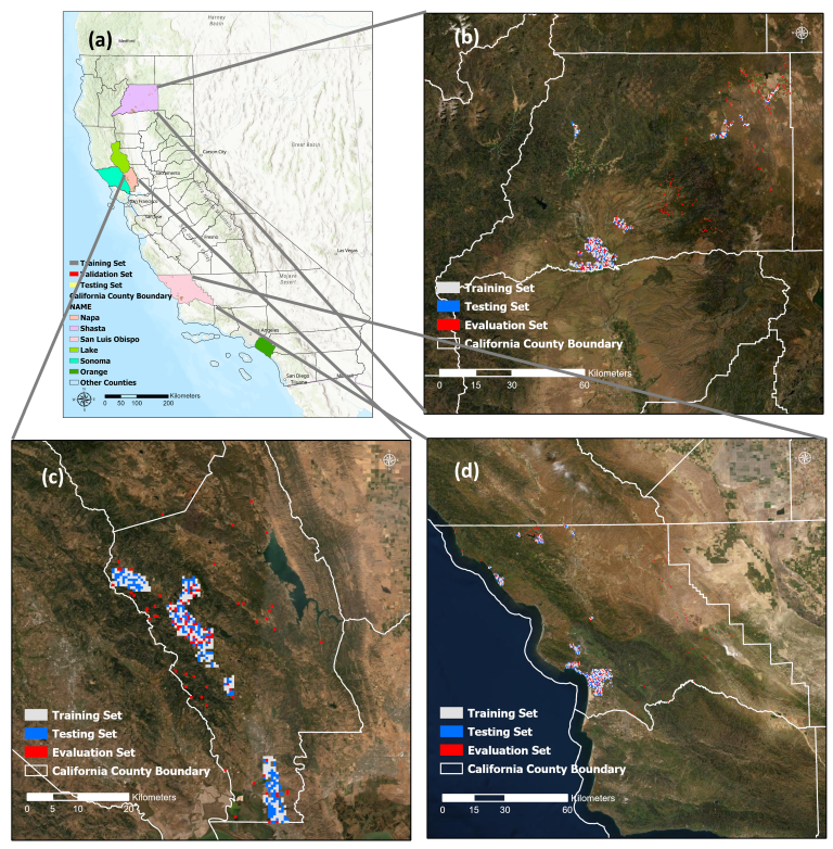
Figure 1. Foci of the study areas (a). NAIP image subsets from three counties, (b) Shasta, (c) Napa, and (d) San Luis Obispo were used to train and test the deep learning model. The model was applied to all NAIP imagery in Lake, Sonoma, and Orange Counties for building detection and WUI mapping every 2 years.
Remotesensing 14 03622 g001
Figure 2. The diagram of the modeling framework for identifying individual building footprint based on the NAIP imagery.
Remotesensing 14 03622 g002
Figure 3. Building footprints detected by our approach over selected sub-regions, representing areas with relatively dense human settlement: (ac) interface WUI and (df) urban areas; and areas with relatively sparse settlements: (gi) intermix WUI and (jl) rural areas. NAIP RGB imagery and the building footprints obtained from county websites are also included for reference and comparison purposes. Locations of these testing subsets are shown in Figure 1.
Remotesensing 14 03622 g003
Figure 4. Building footprints detected by Mobile-UNet (left) and the synthesized approach (middle), respectively, over example areas with dense human settlements (a,b) and sparse human settlements (c,d). The original true color NAIP imagery from the testing set is also shown as a reference (right).
Remotesensing 14 03622 g004
Figure 5. Comparison of building counts aggregated to 300 m resolution from individual building footprints in 2018 by this study (left panel) and Microsoft (right panel) in Lake (a,b), Sonoma (c,d), and Orange Counties (e,f).
Remotesensing 14 03622 g005
Figure 6. Spatial patterns of building counts in Lake County aggregated to 300 m resolution from building footprints identified from the NAIP imagery in (a) 2010 and (c) 2014. Changes in building counts are also shown from 2010 to 2014 (b) and from 2014 to 2018 (d), overlaid with wildfires burned during the corresponding periods. The yellow bounding boxes on Figure 6d indicate locations of example regions in Figure 7.
Remotesensing 14 03622 g006
Figure 7. Examples of tracking building dynamics: (a,b) newly built houses (in black) during 2010–2014 and (c,d) destroyed buildings (in red) by wildfires during 2015-2018 in Lake County. The 2010 buildings were shown at the top in red (a,b) and 2018 postfire buildings in black (c,d). The damaged buildings from the DINS survey were shown in purple for comparison (c,d). Refer to yellow bounding boxes in Figure 6d for the locations of these four examples.
Remotesensing 14 03622 g007
Figure 8. Comparison of WUI maps derived from the 2010 NAIP-based building footprints in this study (a,d,g); from SILVIS 2010 WUI maps (b,e,h); and from the 2018 Microsoft building dataset (c,f,i). Results are shown over Lake County (top), Sonoma County (middle), and Orange County (bottom panel).
Remotesensing 14 03622 g008
Figure 9. Changes in identified WUI areas in Lake County from 2010 to 2018 (ae). Closeups are also shown for a subset region in 2010 (f) and 2018 (g).
Remotesensing 14 03622 g009
Table 1. Performance of different model components in building footprint detection, based on the testing and the evaluation sets, respectively.
AccuracyF1PrecisionRecallIoU
Testing Dataset
Final Model0.970.530.520.540.52
Mobile-UNet Only0.960.410.300.660.43
cGAN only0.880.310.240.400.32
Evaluation Dataset
Final Model0.980.640.650.620.50
Mobile-UNet Only0.970.480.360.700.43
cGAN only0.930.350.490.270.34
Table 2. Evaluation of building footprint mapping with the evaluation dataset at the pixel and individual object level over the whole study area and three counties in California, along the gradient of housing density, i.e., urban, Interface WUI, Intermix WUI, and rural areas, respectively. Moreover, included are the aggregated percentages of building cover from this study and reference data.
Accuracy% Building Area
AccuracyF1PrecisionRecallIoUThis StudyGround Truth
Overall
Urban0.930.610.580.650.537.26%8.83%
Interface WUI0.950.620.620.620.525.12%6.15%
Intermix WUI0.990.670.800.580.471.39%1.47%
Rural0.990.750.890.640.430.39%0.40%
Shasta County
Urban0.950.610.690.550.515.14%6.13%
Interface WUI0.970.620.690.560.513.54%4.61%
Intermix WUI0.990.680.840.580.481.18%1.25%
Rural0.990.760.910.660.440.43%0.42%
Napa County
Urban0.880.580.560.610.509.21%11.82%
Interface WUI0.930.560.570.550.477.39%7.35%
Intermix WUI0.980.600.710.520.442.10%2.07%
Rural0.990.660.860.540.360.36%0.41%
San Luis Obispo County
Urban0.930.620.550.700.547.91%9.62%
Interface WUI0.950.640.570.720.536.75%8.09%
Intermix WUI0.990.700.780.640.481.41%1.60%
Rural0.990.760.860.680.470.31%0.33%
Publisher’s Note: MDPI stays neutral with regard to jurisdictional claims in published maps and institutional affiliations.