Article

Evaluating the Spatial Risk of Bacterial Foodborne Diseases Using Vulnerability Assessment and Geographically Weighted Logistic Regression

1
Zhejiang Provincial Key Laboratory of Urban Wetlands and Regional Change, Hangzhou Normal University, Hangzhou 311121, China
2
Zhejiang Provincial Center for Disease Control and Prevention, Hangzhou 310051, China
3
School of Earth and Planetary Sciences, Curtin University, Perth 6845, Australia
*
Author to whom correspondence should be addressed.
Remote Sens. 2022, 14(15), 3613; https://doi.org/10.3390/rs14153613
Submission received: 5 June 2022 / Revised: 24 July 2022 / Accepted: 26 July 2022 / Published: 28 July 2022
(This article belongs to the Special Issue Remote Sensing and GIS for Monitoring Urbanization and Urban Health)

Abstract

:
Foodborne diseases are an increasing concern to public health; climate and socioeconomic factors influence bacterial foodborne disease outbreaks. We developed an “exposure–sensitivity–adaptability” vulnerability assessment framework to explore the spatial characteristics of multiple climatic and socioeconomic environments, and analyzed the risk of foodborne disease outbreaks in different vulnerable environments of Zhejiang Province, China. Global logistic regression (GLR) and geographically weighted logistic regression (GWLR) models were combined to quantify the influence of selected variables on regional bacterial foodborne diseases and evaluate the potential risk. GLR results suggested that temperature, total precipitation, road density, construction area proportions, and gross domestic product (GDP) were positively correlated with foodborne diseases. GWLR results indicated that the strength and significance of these relationships varied locally, and the predicted risk map revealed that the risk of foodborne diseases caused by Vibrio parahaemolyticus was higher in urban areas (60.6%) than rural areas (20.1%). Finally, distance from the coastline was negatively correlated with predicted regional risks. This study provides a spatial perspective for the relevant departments to prevent and control foodborne diseases.

Graphical Abstract

1. Introduction

Foodborne diseases are infectious or toxic diseases transmitted by the consumption of food [1] and are one of the most significant public health problems worldwide. According to a World Health Organization (WHO) Foodborne Disease Burden Epidemiology Reference Group (FERG) report, 600 million foodborne illnesses and 420,000 deaths were caused by global foodborne hazards in 2010 [2]. In China, studies have shown that 748 million cases of acute gastrointestinal illness and 420 million medical consultations occur annually throughout the country [3]. As a result, foodborne diseases bring significant socioeconomic burdens and hidden dangers to residential health. According to the national foodborne disease molecular tracing network established in 2013, Salmonella species, Vibrio parahaemolyticus, Staphylococcus aureus, and diarrheagenic Escherichia coli are the most common foodborne pathogens that cause outbreaks in China [4]. Among these, V. parahaemolyticus is a halophilic, gram-negative bacterium that has been the leading cause of foodborne disease outbreaks and cases of infectious diarrhea in China, especially in coastal regions [5]. Therefore, it is essential to analyze the influencing factors and risk of foodborne diseases caused by V. parahaemolyticus.
Based on surveillance data, many studies on foodborne diseases have explored their epidemiological characteristics [6,7,8] and many scholars have conducted research on foodborne diseases, such as exploring influencing factors and predicting infection risks [9,10,11,12]. Chen et al. conducted a multivariable logistic regression analysis to analyze the association between food-handling behaviors and foodborne acute gastroenteritis in Anhui, China [9]. Zhang et al. used several machine learning models (e.g., support vector machine, random forest, and XGBoost) to study foodborne disease outbreaks across China and identify their confounding factors [10]. Wang et al. applied a Bayesian nowcasting model to forecast the total daily number of foodborne disease cases [11]. Li et al. used the autoregressive integrated moving average (ARIMA) model to predict foodborne disease incidence in Shenzhen City [12]. However, these studies assumed each factor affected the diseases uniformly, ignoring geographical variations in the influencing factors. As a spatial regression method, geographically weighted logical regression (GWLR) allows the intensity of these factors and their relative importance to vary geographically [13] and has been widely used in epidemiological studies of infectious diseases, such as thrombocytopenia syndrome, dengue, and malaria [14,15,16]. For instance, Zhou et al. found that, compared to the non-spatial logistical regression, the GWLR model offers better understanding of the geographical variations of the risk factors associated with infection of hepatitis C virus [17]. Using GWLR to explore influencing factors can provide a unique spatial perspective.
Vulnerability, which comprises exposure, sensitivity, and adaptability [18], plays a vital role in global environmental change and sustainability research (e.g., flood, heat waves, dengue, and SARS-CoV-2 infections) [19,20,21,22,23]. The concept of vulnerability first appeared in the study of natural hazards [24]. Then it gradually developed into an interdisciplinary and multiscale direction. Adger considered vulnerability as “…the state of susceptibility to harm from exposure to stresses associated with environmental and social change and from the absence of capacity to adapt” [24]. The above definition is widely recognized [25,26,27]. Exposure is defined as the proximity of people or systems to external disturbances [28]. Climate variables, such as temperature and precipitation patterns, extreme weather events, and ocean warming, have complex effects on the food chain, thus affecting the occurrence of foodborne diseases, especially those caused by bacteria. Studies have shown that rising temperatures and heavy rainfall may increase the number of foodborne disease cases [29,30,31]. Sensitivity can be understood as the degree of a system being easily disturbed [26]. The effect of foodborne diseases on crowds varies and the degree of this effect depends on age, sex, food preferences, and food-handling behaviors [32,33]. Osei-Tutu et al. found that the most affected group were those between the ages of 15 and 34 in Accra, Ghana [34]. Moreover, the degree of impact also differs between urban and rural areas; for example, Czerwinski et al. found that the incidence of foodborne botulism among rural residents was more than twice as high as that in urban areas [35]. Adaptability reflects the ability of a system to adapt and adjust to external disturbances [28]. The higher the level of economic medical development, the stronger the ability to deal with health threats. Xiao et al. found that per capita gross domestic product (GDP) was negatively associated with disease incidence [36]. The selection of vulnerability indicators varies depending on the physical attributes of the event; however, few studies have assessed foodborne diseases and vulnerability together. Therefore, we propose a comprehensive foodborne disease vulnerability assessment framework to identify the dominant influencing factors.
Zhejiang Province is an important part of the Yangtze River Delta urban agglomeration, which belongs to the typical subtropical monsoon climate and has a wide variety of aquatic products. Geographical and climatic conditions are suitable for the growth of microorganisms. Among the identified causes of foodborne disease outbreaks, the number of foodborne illnesses caused by bacterial pathogen infections were the largest [6]. Previous evidence has shown that V. parahaemolyticus was responsible for the largest number of outbreaks in Zhejiang Province from 2010 to 2014 [37]. Taking Zhejiang as a case study, this study aimed to screen the influencing factors of foodborne diseases, based on the vulnerability assessment framework, and investigate the specific relationship between these factors and the positive foodborne disease cases caused by V. parahaemolyticus. Furthermore, the GWLR model was combined with foodborne diseases to identify the relative geographical importance of environmental and sociodemographic variables. Finally, we produced a map of the predicted probability of foodborne diseases to determine the spatial epidemiological risk.

2. Materials and Methods

2.1. Study Area

Zhejiang Province is on the southeast coast of China (Figure 1) and covers 101,800 km2 with a long 1805 km zigzag-shaped coastline. It has a subtropical monsoon climate with hydrothermal conditions that are conducive to microorganism growth. The province includes 11 prefecture-level cities and has experienced significant economic development. With rapid socioeconomic development, regional relationships grow closer, and personal dietary structures become richer. Zhejiang Province has a high incidence of foodborne diseases, especially bacterial foodborne diseases caused by V. parahaemolyticus. According to the Zhejiang Province Foodborne Disease Monitoring and Reporting System, the detection rate of foodborne diseases caused by V. parahaemolyticus has recently increased. Zhejiang Province first set up sentinel hospitals to conduct foodborne disease surveillance and reporting in 2010. To ensure that each district and county can be effectively monitored, 101 sentinel hospitals are located in 89 districts and counties in Zhejiang Province. It should be noted that sentinel hospitals were added in areas with a large resident population. However, some problems remain unsolved, such as imperfect monitoring mechanisms, disunity of information construction standards, and inadequate data utilization. Overall, it is essential to more effectively mine information based on existing monitoring data. To carry out more detailed research, we used the ArcGIS fishnet tool to generate the 0.1° × 0.1° grid data.
This study uses the township administrative region as the primary division unit, dividing the study area into urban and rural areas (Figure 1). The division principles were defined based on the “Provisions on Statistical Division of Urban and Rural Areas” designated by the National Bureau of Statistics [38]. Urban areas are those that house municipal district governments and other subdistrict offices under the jurisdiction of the district, along with town governments and other neighborhood committee areas under the jurisdiction of the town. Rural areas refer to the regions outside of these urban areas. Notably, since regular grids and irregular administrative boundaries do not always fit well, some grids required manual judgement when dividing the urban and rural areas according to local knowledge. For example, street administrative divisions are incomplete in a grid. When the proportion of urban administrative areas in a grid was greater than 70%, we defined the grid as an urban area. In short, there was an initial division of urban and rural areas based on the administrative division data of the town, and then a more detailed judgment was made with the help of remote sensing images and local knowledge.

2.2. Data Source

Meteorological data, including dew point temperature, temperature, surface net solar radiation, total precipitation, daily maximum temperature, and daily minimum temperature, were obtained from the European Center for Medium-Range Weather Forecasts (ECMWF).
Road data were derived from OpenStreetMap (https://www.openstreetmap.org (accessed on 23 March 2021)), and the hospital-related points of interest (POI) data were extracted from Amap application programming interface (API). The population density data came from the Gridded Population of the World (https://sedac.ciesin.columbia.edu/data/collection/gpw-v4 (accessed on 23 July 2022)). Based on the Seventh National Census of China in 2020, the population raster data were adjusted [39]. The GDP spatial distribution kilometer grid data, annual normalized difference vegetation index (NDVI), spatial distribution data, and the China land use data were downloaded from the Resource and Environmental Science and Data Center of the Chinese Academy of Sciences (https://www.resdc.cn (accessed on 28 April 2021)).
Data on foodborne diseases caused by V. parahaemolyticus were collected from the “Zhejiang Province Foodborne Disease Surveillance and Reporting System”, which contained data on 31,932 tested cases came from 101 sentinel hospitals in 2018, including attributes of date, gender, age, address, occupation, and detection results.

2.3. Foodborne Diseases Vulnerability Assessment Framework

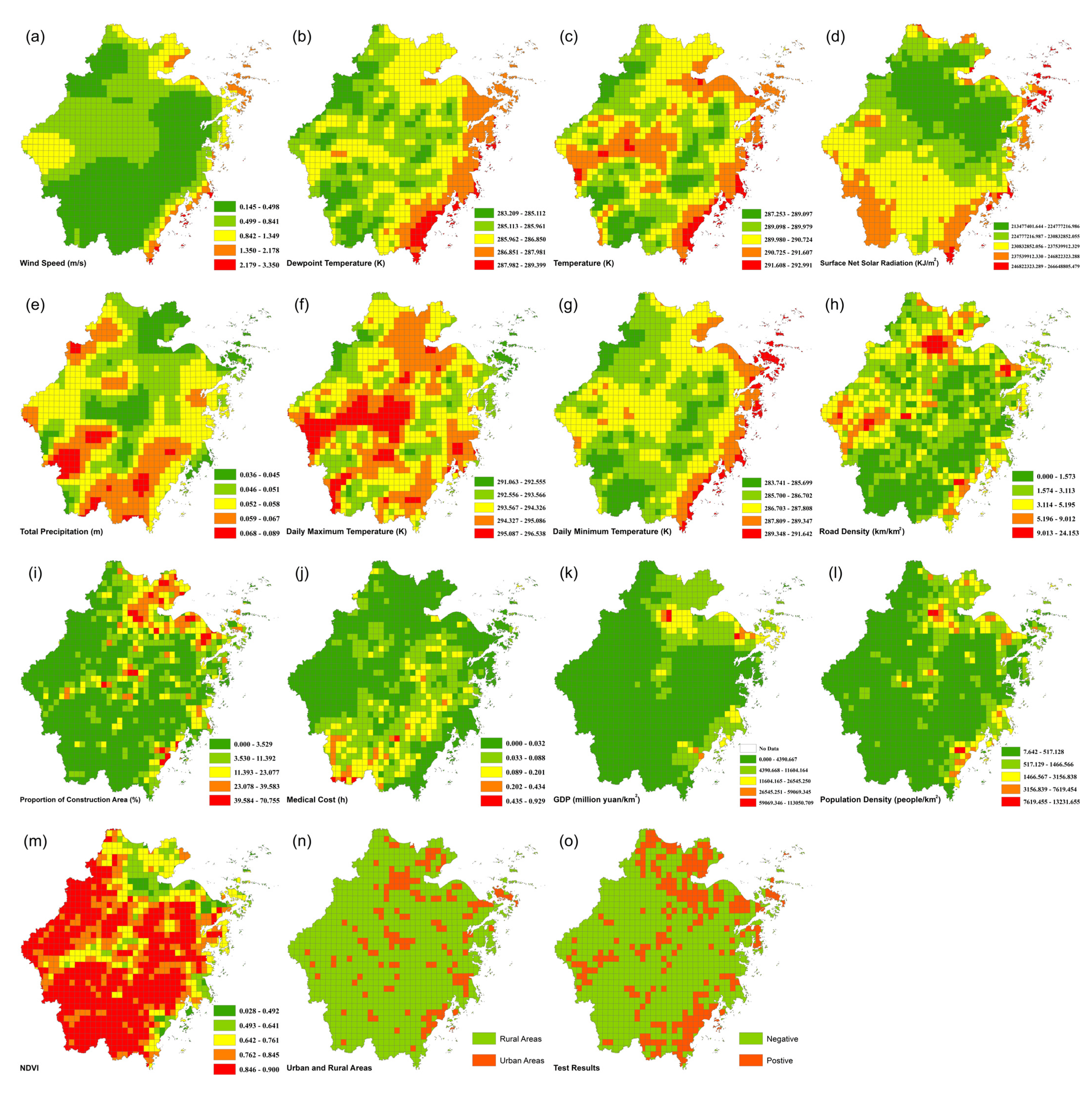
According to the definition of vulnerability, this study proposes an assessment framework for foodborne disease vulnerability based on exposure, sensitivity, and adaptability (Table 1). Previous studies have shown that climate change will have a complex impact on the persistence and dispersal of foodborne pathogens [40]; therefore, our exposure indices here were focused on various meteorological indicators. Urbanization affects consumption patterns and food production processes, which can increase the risk of foodborne diseases [41]; therefore, our sensitivity indices were focused on road density and construction area proportions. As indispensable social resources for combating diseases, hospitals and health institutes are crucial to maintaining personal health [42]. Additionally, medical resources are closely related to regional economic development; therefore, our adaptability indices are focused on regional medical time costs and GDP. The vulnerability of foodborne diseases mentioned in this paper refers to the relationship between the “human–environment” system and foodborne diseases; that is, the susceptibility of the state of the system to harm from exposure to stresses associated with foodborne diseases and from the absence of the capacity to adapt. All data were processed using the same grid size (0.1° × 0.1°) in ArcGIS as shown in Figure 2. The numerical differences among each variable are shown in Table 2.

2.4. Global Logistic Regression

We applied classic logistic regression to explore the relationship between vulnerability to environmental factors and foodborne diseases caused by V. parahaemolyticus. The logistic regression model is a generalized linear model with a binomial distribution for the dependent variable [43]. The dependent variable of the logistic regression in this study was the presence or absence of foodborne disease cases caused by V. parahaemolyticus. When Y = 1, there were positive cases in the grid; otherwise, Y = 0. The independent variables were temperature, total precipitation, road density, proportion of the construction area, distribution of urban and rural areas, and GDP. The classic logistic regression is called global logistic regression (GLR), expressed as follows:
l o g i t Y = β 0 + n = 1 k β n X n + ε
where βn is the regression coefficient of independent variable Xn, β0 is the intercept, logit (Y) is a linear combination function of the covariates, and ε is the error term. To detect and reduce the multicollinearity of these independent variables before regression modeling, we calculated the variance inflation factor (VIF). When VIF > 10, collinearity in the explanatory variables was considered problematic [44,45]. The probability (Y = 1) can be calculated as follows:
P Y = 1 = exp β 0 + n = 1 k β n X n 1 + exp β 0 + n = 1 k β n X n
where P (Y = 1) represents the probability of detecting foodborne disease cases caused by V. parahaemolyticus. Areas with larger probability values represent a higher risk of foodborne diseases. Thus, we can identify the risk of foodborne diseases in the analysis area.

2.5. Geographically Weighted Logistic Regression Model

Figure 2 shows the geospatial heterogeneity of independent and dependent variables. Therefore, using the GWLR model is instrumental for considering the spatial dependence and capturing spatial variations. The GWLR model is a local regression method for investigating spatial non-stationarity [46], and it can explore the variation of the coefficient of each covariate geographically. For GWLR, the variables involved in the operation of the model were the same as those previously described. GWLR model is expressed as follows:
y = β 0 u j , v j + n = 1 k β n u j , v j X n j + ε j
where uj and vj are the spatial coordinates of grid j, βn (uj, vj) is the regression coefficient of the independent variable Xn at location j, and εj is the error term specific to location j. Similar to the GLR model, the probability that (Y = 1) is expressed as follows:
P Y = 1 = exp β 0 u j , v j + n = 1 k β n u j , v j X n j 1 + exp β 0 u j , v j + n = 1 k β n u j , v j X n j
To compare the performances of the GLR and GWLR models, we used the deviance, corrected Akaike information criterion (AICc), and area under the receiver operating characteristic curve (AUC) to evaluate the model fitness and prediction accuracy. For example, the lower the deviance and AICc, the better the model fits the data [47,48]; the higher the AUC, the better the prediction accuracy of the model [47].

3. Results

3.1. Global Logistic Regression

Based on correlation analysis, we eliminated some variables because of the multicollinearity problem. For instance, proportion of construction area, population density, and NDVI were significantly collinear; dewpoint temperature, temperature, and daily minimum temperature were highly correlated. After evaluating the performance of the models from the perspective of collinearity, temperature, total precipitation, road density, proportion of construction area, dummy variable for rural areas, and GDP were included as the dependent variables in the regression model. Table 3 shows that the VIF values of these covariates (VIF = 1.443, 1.412, 1.820, 2.207, 1.503, and 1.456, respectively) are all smaller than the preselected threshold. The results of the GLR model showed that except for dummy variable for rural areas, most selected variables had a significant positive association with foodborne disease cases caused by V. parahaemolyticus (p < 0.05), which indicated that as temperature, total precipitation, road density, construction area proportions, and GDP increased, the probability of a grid converting from negative to positive also increased (Table 3). Furthermore, the positive effects of these independent variables on the presence or absence of foodborne disease cases, from strong to weak, were construction area proportions, GDP, road density, temperature, and total precipitation.

3.2. Geographically Weighted Logistic Regression

To capture geographical spatial variations, we applied GWLR to the same dataset of 964 grids, which showed a clear improvement over the GLR model, as shown in Table 3 and Table 4. While the AICc and deviance values for the GWLR model (AICc = 874.659; deviance = 760.530) were much lower than those of the GLR model (AICc = 952.390; deviance = 938.390), which meant that the GWLR model had a much better model fit, the higher AUC value of the GLR model (AUC = 0.871) compared to that of the GWLR model (AUC = 0.772) suggested that it had a higher prediction accuracy for foodborne diseases.
Parameter estimates and pseudo-t-statistics for each grid were generated using the software package GWR4. The summary descriptive statistics of the local parameter coefficients are shown in Table 4, suggesting that temperature, total precipitation, road density, construction area proportions, and GDP each have negative and positive parameter values. The majority of the local parameter coefficients for all the variables were positive except for the dummy variable for rural areas.
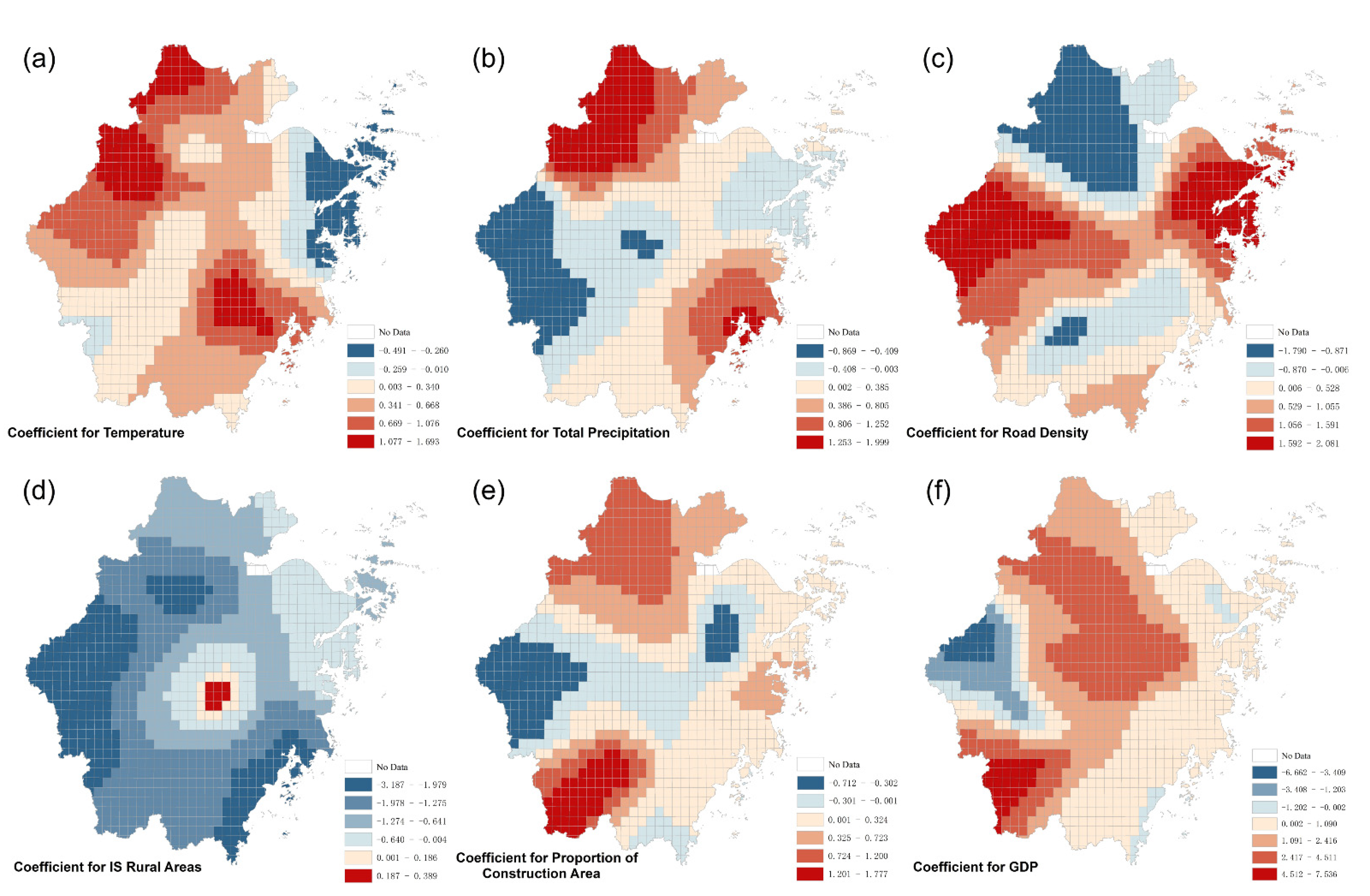
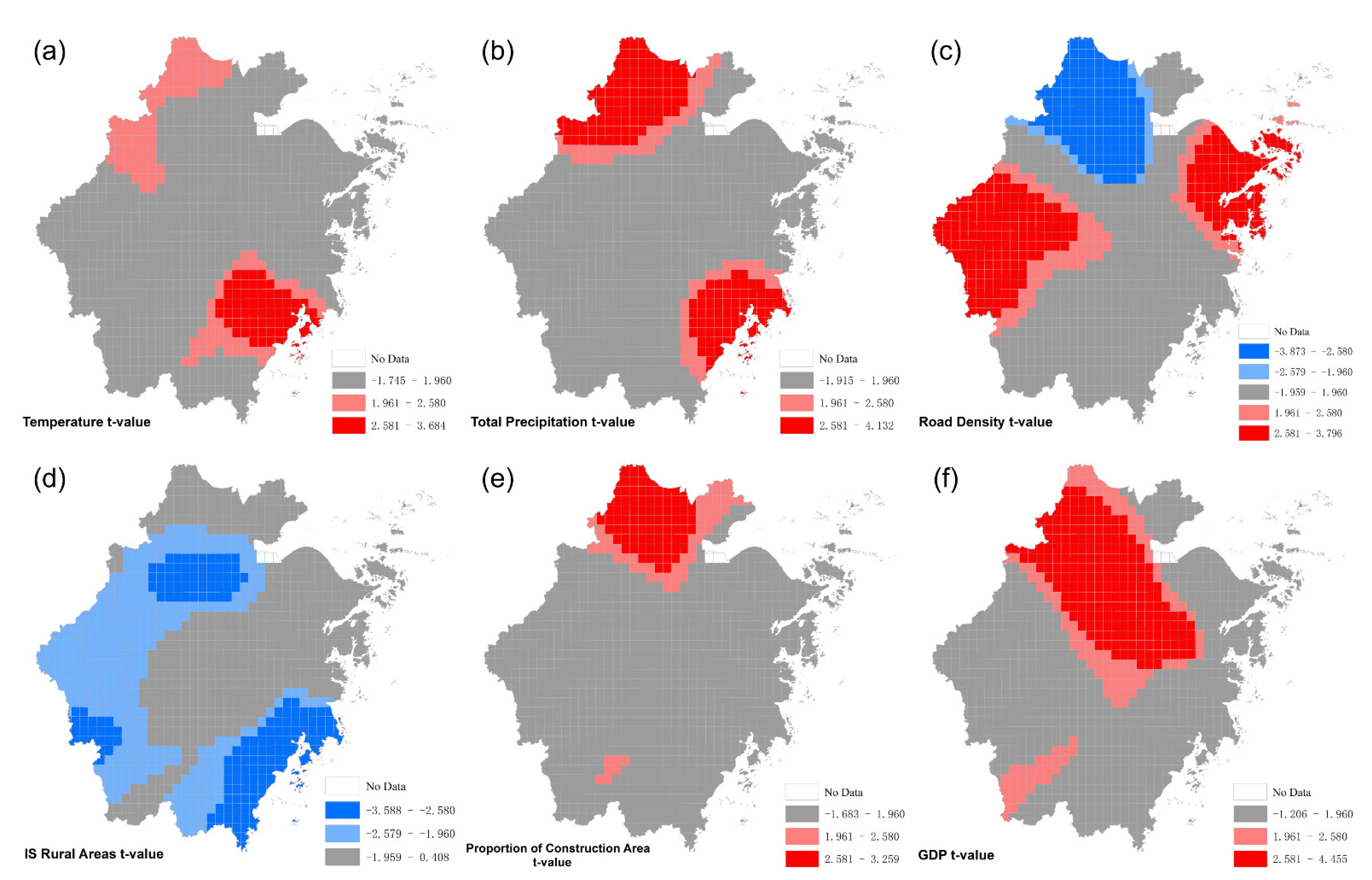
The spatial distributions of the generated coefficients and t-statistics surfaces with a grid size of 0.1° × 0.1° are shown in Figure 3 and Figure 4, respectively. Figure 4 shows that all the selected variables had certain areas where they were not statistically significant. For example, temperature had a significant positive effect on foodborne diseases in the northwestern and southeastern portions of the study area, while total precipitation had a larger significant positive impact area. In significantly affected areas, only the coefficient of road density and rural areas were negative. The construction area proportions had a positive relationship, mainly in the northern regions of the study area. The significantly positive influence areas of GDP extend in a strip from the northwest to the center of Zhejiang Province.

3.3. Mapping the Risk of Foodborne Diseases

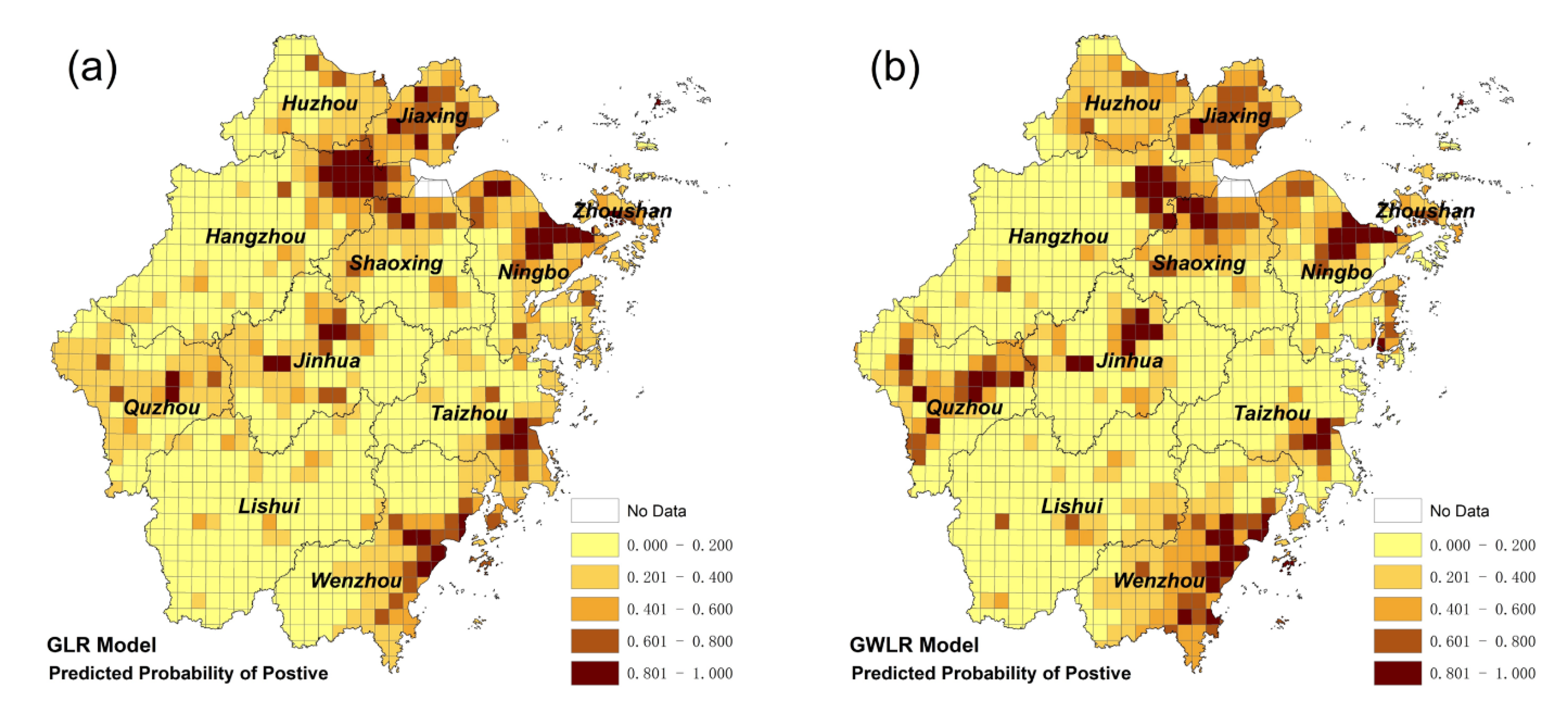
Figure 5 illustrates a map of the predicted probability of foodborne disease infection based on the GLR and GWLR models. We divided the risk of foodborne diseases into five grades, from low to high, based on GWLR. The areas of each risk region were 55.7%, 20.1%, 12.3%, 6.7%, and 5.2%, respectively (Table 5). Moreover, this map indicates that the risks were higher in urban areas (60.6%) than in rural areas (20.1%). Compared with the GLR, the GWLR risk map predicted a higher probability of cases in some regions (e.g., Wenzhou in the southern part of Zhejiang Province) and a lower probability in some areas (e.g., the western part of Hangzhou).
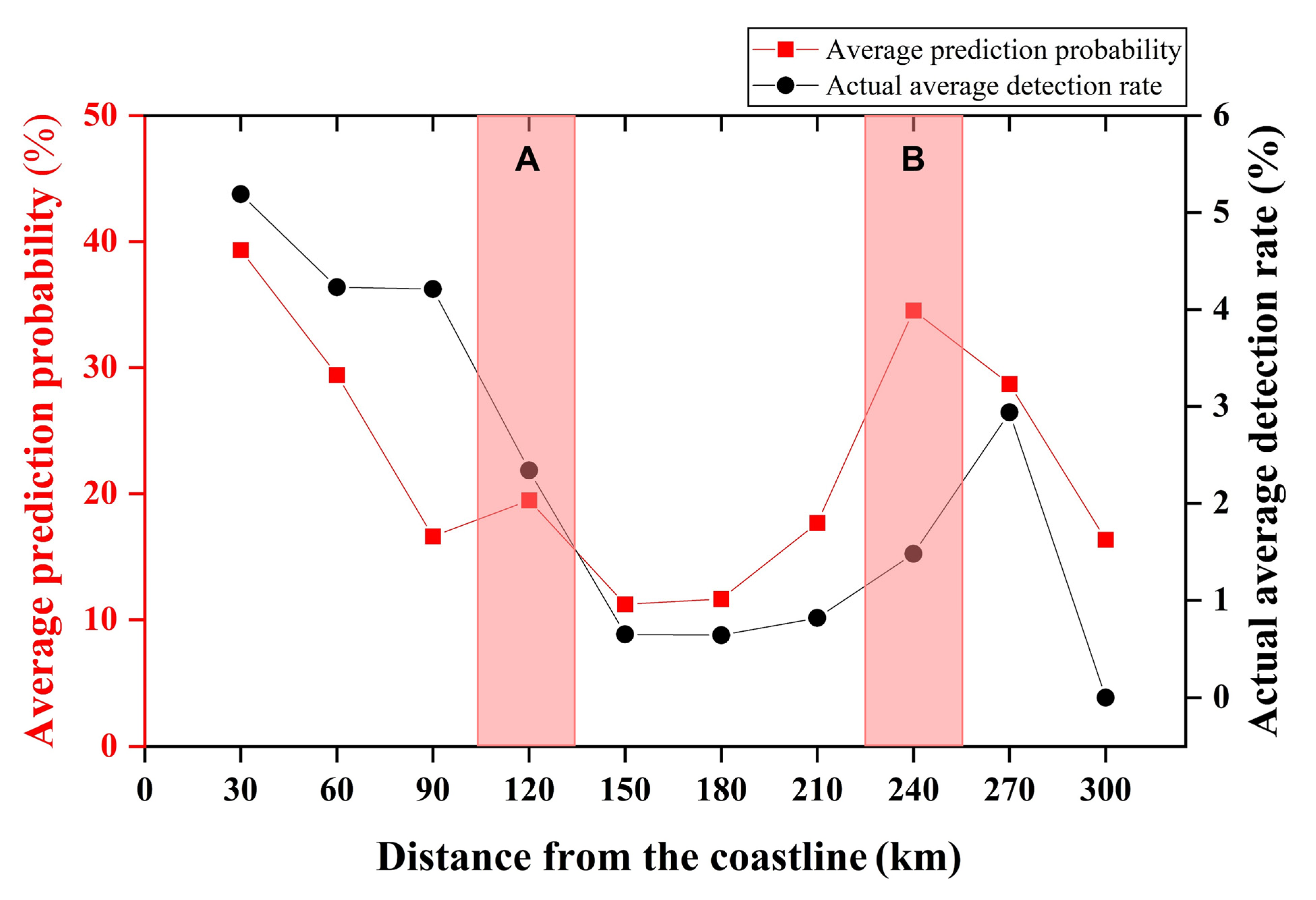
Furthermore, we divided Zhejiang Province into different areas according to their distance from the coastline and calculated the average prediction probability for each area. The calculation results are shown in Figure 6. The changing trend of the prediction probability is similar to that of the actual average detection rate. The distance from the coastline had a negative association with the average prediction probability around Zhejiang Province, except for an area 90–120 km and 180–240 km from the coastline.

4. Discussion

Based on the vulnerability assessment framework and variable screening method, Table 3 and Table 5 show that regional temperature, total precipitation, road density, construction area proportions, rural areas, and GDP have a significant effect on the positive detection of V. parahaemolyticus in the GLR or GWLR models. Positive cases of foodborne diseases were positively correlated with air temperature, which is consistent with the findings of Hsiao et al. [49], who reported similar findings in Taiwan [49]. However, these positive relationships differ from the findings of Shih et al. [50], in that the detection rate of V. parahaemolyticus was negatively correlated with average daily rainfall [50]. One possible reason for this disparity is that the very humid plum rain season occurs in June and July in Zhejiang Province, which brings abundant precipitation, making it easier for bacteria to breed. Road density and construction area proportions also had significant positive effects on foodborne diseases, while the occurrence of rural areas had a negative relationship with positive cases occurrence. It is consistent with the view proposed by Prinsen [41] that urbanization can affect the risk of foodborne diseases. Based on these correlations, urban areas in Zhejiang Province should be more heavily studied than rural areas. Additionally, there was a positive correlation between GDP and foodborne diseases, suggesting that the prevention and control of foodborne diseases should not be neglected when pursuing economic development. However, this differed from the findings of Yang et al. [51], who reported that the incidence of foodborne diseases had a negative correlation with GDP in Jinan. This discrepancy could be because the attitudes and behavior of foodborne disease patients in choosing healthcare vary due to different socioeconomic and cultural backgrounds; for example, rural residents are less likely to visit hospitals when they suffer from foodborne diseases.
The GLR model ignores geographical variations in the relationships between the dependent variable and covariates, whereas the GWLR model can detect this spatial variability [52]. Temperature and total precipitation only showed significant positive effects in some areas of northwest and southeast Zhejiang. The mostly non-significant relationship and differences from others may have been a consequence of the spatiotemporal scales of the meteorological data. A significant and positive relationship between road density and the presence or absence of positive cases was found in the western and eastern regions, while an outlier occurred in northern Zhejiang, and there was a negative correlation between road density and V. parahaemolyticus detection rate. Although the developed road network can promote food transportation, the supervision of food hygiene quality in these areas near the main urban area of the provincial capital city is more stringent, and the daily dietary hygiene habits of residents are healthier. The proportion of construction area had a positive relationship, predominantly in the northern and southwestern parts of the study area. Furthermore, the rural areas had a significant negative relationship in the west and southeast of Zhejiang Province. The significantly positive influence area of GDP extends in a strip from the northwest to the center of Zhejiang Province. The coefficients and significance of the proportion of construction areas and GDP varied geographically. The influence of these factors on foodborne diseases caused by V. parahaemolyticus varied geographically. Furthermore, our findings verify that GWLR can provide improvements and additional perspectives over classic non-spatial regression models for eco epidemiological studies on bacterial foodborne diseases [53]. As the relative importance of each independent variable differed geographically, public health practitioners can identify the most important influencing factors and develop public health interventions for various regions more precisely.
GWLR had more advantages in model performance compared to GLR. Owing to the spatial heterogeneity of the driving mechanism, non-spatial regression models may perform poorly [54]. A comparison of the model performances between the GLR and GWLR is shown in Table 3 and Table 4. The AICc and deviance values of GWLR were 874.659 and 760.530, respectively, which were lower than those of the GLR model, indicating that GWLR performed better than the GLR model in quantifying the impact of selected variables on foodborne diseases. Additionally, the AUC of GWLR was 0.871, which was much larger than that of the GLR model, suggesting that GWLR had higher prediction accuracy for the probability of positive foodborne disease cases. The evaluation indices of the GWLR model were all better than those of the GLR model, similar to the findings of previous studies [53,55], suggesting that the influence of spatial geographical location on the results of the dependent variables should be considered when fitting data with spatial structure. However, this GWLR approach used the annual total value or average value of covariables to model the relationship between V. parahaemolyticus detection information and vulnerability environmental factors in different regions, ignoring the seasonal variation characteristics of foodborne diseases. It is difficult to predict the epidemic trends of foodborne diseases according to the climate change and other risk factors. Similar to the study on the spatial trends in Salmon infection in Spain [56], we paid attention to the geospatial variation of bacterial pathogen detection, and confirmed the existence of the spatial difference in the risk of bacterial pathogen infection at the province level or grid level. Under the constraints of limited resource input and environmental improvement, it is important to evaluate the spatial risk of V. parahaemolyticus infection in Zhejiang province to help develop local public health strategies, which is the main contribution of this study.
According to the predicted risk maps of foodborne diseases caused by V. parahaemolyticus (Figure 5), the prediction probability in urban areas (60.6%) was higher than that in the rural areas (20.1%). One reason for this phenomenon is that the percentage of seafood intake is lower in rural residents than in urban residents [57]. Outbreaks of foodborne diseases caused by V. parahaemolyticus are associated with dietary habits of seafood consumption. V. parahaemolyticus foodborne disease risks differed between urban and rural areas, which have also been reported by other researchers; for example, using simple linear regression and locally weighted regression, Ford et al. found significantly higher rates of V. parahaemolyticus serotype typhimurium in urban areas than rural areas [58]. Therefore, relevant departments should pay more attention to urban areas than to rural areas. Stricter food regulations, such as the step-by-step seafood safety regulations in Japan, from the production to the consumption stages, are recommended [59]. Considering factors such as medical distance and cost, there are also patients in rural areas who do not visit the hospital after falling ill. Therefore, the monitoring, prevention, and control of foodborne diseases requires efforts from both urban and rural departments.
However, not all urban areas have high prediction probabilities and not all rural areas have low prediction probabilities; for example, the prediction probability of the coastal areas that belonged to rural areas in the northeast and southeast of Zhejiang Province was also high, whereas the prediction probability of some grids belonging to urban areas in the middle of Zhejiang Province was low. Additionally, Figure 6 shows that, as the distance from the coast increased, the prediction probability decreased overall, except for some regions, which was consistent with a study conducted in the littoral domain, where V. parahaemolyticus caused outbreaks of most foodborne diseases [6]. One possible reason for the high prediction probability in inland areas is that V. parahaemolyticus is occasionally detected in other foods. Remarkably, V. parahaemolyticus contamination has been found at a high rate in aquatic products as well as in ready-to-eat (RTE) foods, such as cooked meat, roasted poultry, and cold vegetable dishes in sauce, which are popular in China [60]. Jinhua, 90–180 km from the coastline, is famous for its traditional pickled food, Jinhua ham; Quzhou, 210–270 km from the coastline, is famous for its special stewed meat. Therefore, relevant departments should not ignore other foods while addressing seafood contamination.

5. Conclusions

In this study, we proposed a foodborne disease vulnerability assessment framework, and foodborne disease vulnerability environments were comprehensively described using various types of geographic data. This study combined the GWLR model with foodborne diseases for the first time to analyze the spatial epidemiological risk of foodborne diseases caused by V. parahaemolyticus.
We found that temperature, total precipitation, road density, the proportion of construction area, and GDP are important environmental indicators that affect foodborne diseases. Additionally, the GWLR model had better model fitness and higher prediction accuracy than the GLR model. Compared with the GLR model, the GWLR model can consider the spatial heterogeneity of selected independent variables and their relative geographical importance. The significant relationship between foodborne diseases and these covariates was mostly positive throughout Zhejiang Province, except that road density also had a negative relationship in the northern part of the study area. Furthermore, our model can effectively predict the foodborne disease risks, and our predicted risk map showed that urban areas had a higher overall probability of positive cases. Although foodborne diseases caused by V. parahaemolyticus are related to the distance from the coastline, the supervision of food and residential dietary hygiene habits also contributed to an increased risk of foodborne diseases. Generally, this study provides guidance and geographical support for relevant government departments to prevent and control foodborne diseases in Zhejiang Province.
The limitations and future perspectives should be addressed to better understand these findings. First, urban and rural divisions in this study were based on administrative divisions, and a mixed area may still exist. Determining how to divide urban and rural areas more effectively would be instrumental for future work. Second, the spatiotemporal resolutions of meteorological and socio-economic data limit the spatial scale and neglects seasonal changes in the results. Except for meteorological data, other vulnerability environmental assessment data show the annual average distribution of factors in each region, which are cross-sectional data. Future studies should include higher spatial resolution and dynamically changing time-series data, and then carry out spatiotemporal risk prediction research. Third, the proposed foodborne disease vulnerability assessment framework must be further improved. Based on the perspective of exposure, sensitivity, and adaptability, related information such as age structure, food consumption structure, and fiscal medical hygienic expenditure to the index framework should be included in future studies, aiming to describe the vulnerability of the Zhejiang Province environments from a more comprehensive perspective.

Author Contributions

Conceptualization, W.B. and T.L.; methodology, W.B., H.H., B.Z., and T.L.; software, W.B.; validation, J.C. and S.X.; formal analysis, W.B., H.H., and T.L.; investigation, J.C., W.B., and T.L.; resources, J.C.; data curation, W.B. and T.L.; writing—original draft preparation, W.B. and B.Z.; writing—review and editing, H.H. and J.X.; visualization, W.B.; supervision, H.H. and T.L.; project administration, T.L.; funding acquisition, T.L. All authors have read and agreed to the published version of the manuscript.

Funding

This research was funded by Hangzhou Science and Technology Development Plan (Grant No. 20201203B141), the National Natural Science Foundation of China (Grant No. 41101371).

Data Availability Statement

The data used to support the findings of this study are available from the corresponding author upon request.

Acknowledgments

The authors would like to thank of Zhejiang Provincial Center for Disease Control and Prevention for providing data for the study.

Conflicts of Interest

The authors declare no conflict of interest. The funders had no role in the design of the study; in the collection, analyses, or interpretation of data; in the writing of the manuscript, or in the decision to publish the results.

References

  1. World Health Organization. Foodborne Disease Outbreaks: Guidelines for Investigation and Control; World Health Organization: Geneva, Switzerland, 2008. [Google Scholar]
  2. World Health Organization. WHO Estimates of the Global Burden of Foodborne Diseases: Foodborne Disease Burden Epidemiology Reference Group 2007–2015; World Health Organization: Geneva, Switzerland, 2015. [Google Scholar]
  3. Chen, Y.; Yan, W.; Zhou, Y.; Zhen, S.; Zhang, R.; Chen, J.; Liu, Z.; Cheng, H.; Liu, H.; Duan, S.; et al. Burden of Self-reported Acute Gastrointestinal Illness in China: A Population-based Survey. BMC Public Health 2013, 13, 456. [Google Scholar] [CrossRef] [Green Version]
  4. Li, W.; Wu, S.; Fu, P.; Liu, J.; Han, H.; Bai, L.; Pei, X.; Li, N.; Liu, X.; Guo, Y. National Molecular Tracing Network for Foodborne Disease Surveillance in China. Food Control 2018, 88, 28–32. [Google Scholar] [CrossRef]
  5. Pang, R.; Li, Y.; Chen, M.; Zeng, H.; Lei, T.; Zhang, J.; Ding, Y.; Wang, J.; Wu, S.; Ye, Q.; et al. A Database for Risk Assessment and Comparative Genomic Analysis of Foodborne Vibrio Parahaemolyticus in China. Sci. Data 2020, 7, 321. [Google Scholar] [CrossRef] [PubMed]
  6. Chen, L.; Sun, L.; Zhang, R.; Liao, N.; Qi, X.; Chen, J. Surveillance for Foodborne Disease Outbreaks in Zhejiang Province, China, 2015–2020. BMC Public Health 2022, 22, 135. [Google Scholar] [CrossRef]
  7. Swoveland, J.L.; Stewart, L.K.; Eckmann, M.K.; Gee, R.; Allen, K.J.; Vandegrift, C.M.; Olson, G.; Kang, M.G.; Tran, M.L.; Melius, E.; et al. Laboratory Review of Foodborne Disease Investigations in Washington State 2007–2017. Foodborne Pathog. Dis. 2019, 16, 513–523. [Google Scholar] [CrossRef] [PubMed] [Green Version]
  8. Lee, J.K.; Kwak, N.S.; Kim, H.J. Systemic Analysis of Foodborne Disease Outbreak in Korea. Foodborne Pathog. Dis. 2016, 13, 101–107. [Google Scholar] [CrossRef] [PubMed]
  9. Chen, Y.J.; Wen, Y.F.; Song, J.G.; Chen, B.F.; Ding, S.S.; Ding, L.; Dai, J.J. The Correlation Between Family Food Handling Behaviors and Foodborne Acute Gastroenteritis: A Community-oriented, Population-based Survey in Anhui, China. BMC Public Health 2018, 18, 1290. [Google Scholar] [CrossRef] [PubMed]
  10. Zhang, P.; Cui, W.; Wang, H.; Du, Y.; Zhou, Y. High-Efficiency Machine Learning Method for Identifying Foodborne Disease Outbreaks and Confounding Factors. Foodborne Pathog. Dis. 2021, 18, 590–598. [Google Scholar] [CrossRef] [PubMed]
  11. Wang, X.L.; Zhou, M.Q.; Jia, J.Z.; Geng, Z.; Xiao, G.X. A Bayesian Approach to Real-Time Monitoring and Forecasting of Chinese Foodborne Diseases. Int. J. Environ. Res. Public Health 2018, 15, 1740. [Google Scholar] [CrossRef] [PubMed] [Green Version]
  12. Li, S.; Peng, Z.; Zhou, Y.; Zhang, J. Time Series Analysis of Foodborne Diseases During 2012–2018 in Shenzhen, China. J. Consum. Prot. Food Saf. 2021, 17, 83–91. [Google Scholar] [CrossRef]
  13. Lesiv, M.; Moltchanova, E.; Schepaschenko, D.; See, L.; Shvidenko, A.; Comber, A.; Fritz, S. Comparison of Data Fusion Methods Using Crowdsourced Data in Creating a Hybrid Forest Cover Map. Remote Sens. 2016, 8, 261. [Google Scholar] [CrossRef] [Green Version]
  14. Yasuo, K.; Nishiura, H. Spatial Epidemiological Determinants of Severe Fever with Thrombocytopenia Syndrome in Miyazaki, Japan: A GWLR Modeling Study. BMC Infect. Dis. 2019, 19, 498. [Google Scholar] [CrossRef] [PubMed] [Green Version]
  15. Imran, M.; Hamid, Y.; Mazher, A.; Ahmad, S.R. Geo-spatially Modelling Dengue Epidemics in Urban Cities: A Case Study of Lahore, Pakistan. Geocarto. Int. 2021, 36, 197–211. [Google Scholar] [CrossRef]
  16. Manyangadze, T.; Mavhura, E.; Mudavanhu, C.; Pedzisai, E. An Exploratory Analysis of the Spatial Variation of Malaria Cases and Associated Household Socio-economic Factors in Flood-prone Areas of Mbire district, Zimbabwe. GeoJournal 2021, 1–16. [Google Scholar] [CrossRef]
  17. Zhou, Y.B.; Wang, Q.X.; Yang, M.X.; Gong, Y.H.; Yang, Y.; Nie, S.J.; Liang, S.; Nan, L.; Coatsworth, A.; Yang, A.H.; et al. Geographical variations of risk factors associated with HCV infection in drug users in southwestern China. Epidemiol. Infect. 2016, 144, 1291–1300. [Google Scholar] [CrossRef] [PubMed] [Green Version]
  18. Birch, E.L. Climate Change 2014: Impacts, Adaptation, and Vulnerability. J. Am. Plann. Assoc. 2014, 80, 184–185. [Google Scholar] [CrossRef]
  19. Rathi, S.K.; Chakraborty, S.; Mishra, S.K.; Dutta, A.; Nanda, L. A Heat Vulnerability Index: Spatial Patterns of Exposure, Sensitivity and Adaptive Capacity for Urbanites of Four Cities of India. Int. J. Environ. Res. Public Health 2022, 19, 283. [Google Scholar] [CrossRef]
  20. Udayanga, L.; Gunathilaka, N.; Iqbal, M.C.M.; Abeyewickreme, W. Climate Change Induced Vulnerability and Adaption for Dengue Incidence in Colombo and Kandy Districts: The Detailed Investigation in Sri Lanka. Infect. Dis. Poverty 2020, 9, 102. [Google Scholar] [CrossRef] [PubMed]
  21. De Andrade, M.M.N.; Szlafsztein, C.F. Vulnerability Assessment Including Tangible and Intangible Components in the Index Composition: An Amazon Case Study of Flooding and Flash Flooding. Sci. Total Environ. 2018, 630, 903–912. [Google Scholar] [CrossRef] [PubMed]
  22. Mitrica, B.; Mocanu, I.; Grigorescu, I.; Dumitrascu, M.; Pistol, A.; Damian, N.; Serban, P.R. Population Vulnerability to the SARS-CoV-2 Virus Infection. A County-Level Geographical-Methodological Approach in Romania. GeoHealth 2021, 5, e2021GH000461. [Google Scholar] [CrossRef] [PubMed]
  23. Ahmad, I.; Wang, X.; Waseem, M.; Zaman, M.; Aziz, F.; Khan, R.Z.N.; Ashraf, M. Flood Management, Characterization and Vulnerability Analysis Using an Integrated RS-GIS and 2D Hydrodynamic Modelling Approach: The Case of Deg Nullah, Pakistan. Remote Sens. 2022, 14, 2138. [Google Scholar] [CrossRef]
  24. Adger, W.N. Vulnerability. Glob. Environ. Change 2006, 16, 268–281. [Google Scholar] [CrossRef]
  25. Zhang, Y.; Shen, J.; Li, Y. Atmospheric Environment Vulnerability Cause Analysis for the Beijing-Tianjin-Hebei Metropolitan Region. Int. J. Environ. Res. Public Health 2018, 15, 128. [Google Scholar] [CrossRef] [PubMed] [Green Version]
  26. Chen, Y.; Liu, T.; Ge, Y.; Xia, S.; Yuan, Y.; Li, W.; Xu, H. Examining Social Vulnerability to Flood of Affordable Housing Communities in Nanjing, China: Building Long-term Disaster Resilience of Low-income Communities. Sustain. Cities Soc. 2021, 71, 102939. [Google Scholar] [CrossRef]
  27. Swami, D.; Parthasarathy, D. Dynamics of Exposure, Sensitivity, Adaptive Capacity and Agricultural Vulnerability at District Scale for Maharashtra, India. Ecol. Indic. 2021, 121, 107206. [Google Scholar] [CrossRef]
  28. He, C.; Ma, L.; Zhou, L.; Kan, H.; Zhang, Y.; Ma, W.; Chen, B. Exploring the Mechanisms of Heat Wave Vulnerability at the Urban Scale Based on the Application of Big Data and Artificial Societies. Environ. Int. 2019, 127, 573–583. [Google Scholar] [CrossRef]
  29. Morral-Puigmal, C.; Martinez-Solanas, E.; Villanueva, C.M.; Basagana, X. Weather and Gastrointestinal Disease in Spain: A Retrospective Time Series Regression Study. Environ. Int. 2018, 121, 649–657. [Google Scholar] [CrossRef] [PubMed]
  30. Kim, Y.S.; Park, K.H.; Chun, H.S.; Choi, C.; Bahk, G.J. Correlations Between Climatic Conditions and Foodborne Disease. Food Res. Int. 2015, 68, 24–30. [Google Scholar] [CrossRef]
  31. Bari, L.; Yeasmin, S.; Kawamoto, S. Impact of Climate Change on Foodborne Pathogens and Diseases. J. Jpn. Soc. Food. Sci. 2008, 55, 264–269. [Google Scholar] [CrossRef] [Green Version]
  32. Strassle, P.D.; Gu, W.; Bruce, B.B.; Gould, L.H. Sex and Age Distributions of Persons in Foodborne Disease Outbreaks and Associations with Food Categories. Epidemiol. Infect. 2019, 147, e200. [Google Scholar] [CrossRef] [Green Version]
  33. Chen, Y.J.; Wen, Y.F.; Song, J.G.; Chen, B.F.; Wang, L.; Ding, S.S.; Ding, L.; Dai, J.J. Food Handling Behaviors Associated with Reported Acute Gastrointestinal Disease That May Have Been Caused by Food. J. Food Prot. 2019, 82, 494–500. [Google Scholar] [CrossRef] [PubMed]
  34. Osei-Tutu, B.; Anto, F. Trends of Reported Foodborne Diseases at the Ridge Hospital, Accra, Ghana: A Retrospective Review of Routine Data from 2009–2013. BMC Infect. Dis. 2016, 16, 139. [Google Scholar] [CrossRef] [Green Version]
  35. Czerwinski, M.; Czarkowski, M.P.; Kondej, B. Foodborne Botulism in Poland in 2017. Prz. Epidemiol. 2019, 73, 445–450. [Google Scholar] [CrossRef]
  36. Xiao, G.X.; Xu, C.D.; Wang, J.F.; Yang, D.Y.; Wang, L. Spatial-temporal Pattern and Risk Factor Analysis of Bacillary Dysentery in the Beijing-Tianjin-Tangshan Urban Region of China. BMC Public Health 2014, 14, 998. [Google Scholar] [CrossRef] [PubMed] [Green Version]
  37. Chen, J.; Zhang, R.; Qi, X.; Zhou, B.; Wang, J.; Chen, Y.; Zhang, H. Epidemiology of Foodborne Disease Outbreaks Caused by Vibrio Parahaemolyticus During 2010–2014 in Zhejiang Province, China. Food Control 2017, 77, 110–115. [Google Scholar] [CrossRef]
  38. National Bureau of Statistics of China. Provisions on the Statistical Division of Urban and Rural Areas (for Trial Implementation). Available online: http://www.stats.gov.cn/tjsj/pcsj/rkpc/5rp/html/append7.htm (accessed on 22 December 2021).
  39. Bai, H.M.; Shi, Y.L.; Seong, M.S.; Gao, W.K.; Li, Y.H. Influence of Spatial Resolution on Satellite-Based PM2.5 Estimation: Implications for Health Assessment. Remote Sens. 2022, 14, 2933. [Google Scholar] [CrossRef]
  40. Hellberg, R.S.; Chu, E. Effects of Climate Change on the Persistence and Dispersal of Foodborne Bacterial Pathogens in the Outdoor Environment: A review. Crit. Rev. Microbiol. 2016, 42, 548–572. [Google Scholar] [CrossRef] [PubMed]
  41. Prinsen, G.; Benschop, J.; Cleaveland, S.; Crump, J.A.; French, N.P.; Hrynick, T.A.; Mariki, B.; Mmbaga, B.T.; Sharp, J.P.; Swai, E.S.; et al. Meat Safety in Tanzania’s Value Chain: Experiences, Explanations and Expectations in Butcheries and Eateries. Int. J. Environ. Res. Public Health 2020, 17, 82833. [Google Scholar] [CrossRef] [PubMed]
  42. Cutter, S.L.; Finch, C. Temporal and Spatial Changes in Social Vulnerability to Natural Hazards. Proc. Natl. Acad. Sci. USA 2008, 105, 2301–2306. [Google Scholar] [CrossRef] [Green Version]
  43. Wu, W.; Zhang, L. Comparison of Spatial and Non-spatial Logistic Regression Models for Modeling the Occurrence of Cloud Cover in North-eastern Puerto Rico. Appl. Geogr. 2013, 37, 52–62. [Google Scholar] [CrossRef]
  44. Zuur, A.F.; Ieno, E.N.; Elphick, C.S. A Protocol for Data Exploration to Avoid Common Statistical Problems. Methods Ecol. Evol. 2010, 1, 3–14. [Google Scholar] [CrossRef]
  45. Ye, X.P.; Yu, X.P.; Wang, T.J. Investigating Spatial Non-stationary Environmental Effects on the Distribution of Giant Pandas in the Qinling Mountains, China. Glob. Ecol. Conserv. 2020, 21, e00894. [Google Scholar] [CrossRef]
  46. Lu, B.; Charlton, M.; Harris, P.; Fotheringham, A.S. Geographically Weighted Regression with a Non-Euclidean Distance Metric: A Case Study Using Hedonic House Price Data. Int. J. Geogr. Inf. Sci. 2014, 28, 660–681. [Google Scholar] [CrossRef]
  47. Han, H.; Jang, K.-M.; Chung, J.-S. Selecting Suitable Sites for Mountain Ginseng (Panax ginseng) Cultivation by Using Geographically Weighted Logistic Regression. J. Mt. Sci. 2017, 14, 492–500. [Google Scholar] [CrossRef]
  48. Yang, L.; Yu, K.; Ai, J.; Liu, Y.; Yang, W.; Liu, J. Dominant Factors and Spatial Heterogeneity of Land Surface Temperatures in Urban Areas: A Case Study in Fuzhou, China. Remote Sens. 2022, 14, 1266. [Google Scholar] [CrossRef]
  49. Hsiao, H.I.; Jan, M.S.; Chi, H.J. Impacts of Climatic Variability on Vibrio Parahaemolyticus Outbreaks in Taiwan. Int. J. Environ. Res. Public Health 2016, 13, 20188. [Google Scholar] [CrossRef] [Green Version]
  50. Shih, Y.J.; Chen, J.S.; Chen, Y.J.; Yang, P.Y.; Kuo, Y.J.; Chen, T.H.; Hsu, B.M. Impact of Heavy precipitation Events on Pathogen Occurrence in Estuarine Areas of the Puzi River in Taiwan. PLoS ONE 2021, 16, e0256266. [Google Scholar] [CrossRef]
  51. Yang, L.; Sun, Y.B.; Zhong, Q.; Duan, D.S.; Liu, S.Q.; Zhang, Y. Epidemiological Characteristics and Spatio-temporal Patterns of Foodborne Diseases in Jinan, Northern China. Biomed. Environ. Sci. 2019, 32, 309–313. [Google Scholar] [CrossRef]
  52. Zhang, L.; Wei, Y.; Meng, R. Spatiotemporal Dynamics and Spatial Determinants of Urban Growth in Suzhou, China. Sustainability 2017, 9, 30393. [Google Scholar] [CrossRef] [Green Version]
  53. Mayfield, H.J.; Lowry, J.H.; Watson, C.H.; Kama, M.; Nilles, E.J.; Lau, C.L. Use of Geographically Weighted Logistic Regression to Quantify Spatial Variation in the Environmental and Sociodemographic Drivers of Leptospirosis in Fiji: A Modelling Study. Lancet Planet. Health 2018, 2, 223–232. [Google Scholar] [CrossRef]
  54. Li, H.; Peng, J.; Yanxu, L.; Yi’na, H. Urbanization Impact on Landscape Patterns in Beijing City, China: A Spatial Heterogeneity Perspective. Ecol. Indic. 2017, 82, 50–60. [Google Scholar] [CrossRef]
  55. Clary, C.; Lewis, D.J.; Flint, E.; Smith, N.R.; Kestens, Y.; Cummins, S. The Local Food Environment and Fruit and Vegetable Intake: A Geographically Weighted Regression Approach in the ORiEL Study. Am. J. Epidemiol. 2016, 184, 837–846. [Google Scholar] [CrossRef] [PubMed]
  56. Teng, K.T.Y.; Aviles, M.M.; Ugarte-Ruiz, M.; Barcena, C.; de la Torre, A.; Lopez, G.; Moreno, M.A.; Dominguez, L.; Alvarez, J. Spatial Trends in Salmonella Infection in Pigs in Spain. Front. Vet. Sci. 2020, 7, 345. [Google Scholar] [CrossRef] [PubMed]
  57. Yan, Y.; You, L.; Wang, X.; Zhang, Z.; Li, F.; Wu, H.; Wu, M.; Zhang, J.; Wu, J.; Chen, C.; et al. Iodine Nutritional Status, the Prevalence of Thyroid Goiter and Nodules in Rural and Urban Residents: A Cross-sectional Study from Guangzhou, China. Endocr. Connect. 2021, 10, 1550–1559. [Google Scholar] [CrossRef] [PubMed]
  58. Ford, M.W.; Odoi, A.; Majowicz, S.E.; Michel, P.; Middleton, D.; Ciebin, B.; Dore, K.; McEwen, S.A.; Aramini, J.A.; Deeks, S.; et al. A Descriptive Study of Human Salmonella Serotype Typhimurium Infections Reported in Ontario from 1990 to 1998. Can. J. Infect. Dis. Med. Microbiol. 2003, 14, 267–273. [Google Scholar] [CrossRef] [Green Version]
  59. Hara-Kudo, Y.; Kumagai, S. Impact of Seafood Regulations for Vibrio Parahaemolyticus Infection and Verification by Analyses of Seafood Contamination and Infection. Epidemiol. Infect. 2014, 142, 2237–2247. [Google Scholar] [CrossRef] [PubMed]
  60. Xie, T.; Xu, X.; Wu, Q.; Zhang, J.; Cheng, J. Prevalence, Molecular Characterization, and Antibiotic Susceptibility of Vibrio Parahaemolyticus from Ready-to-Eat Foods in China. Front. Microbiol. 2016, 7, 17–23. [Google Scholar] [CrossRef] [PubMed]
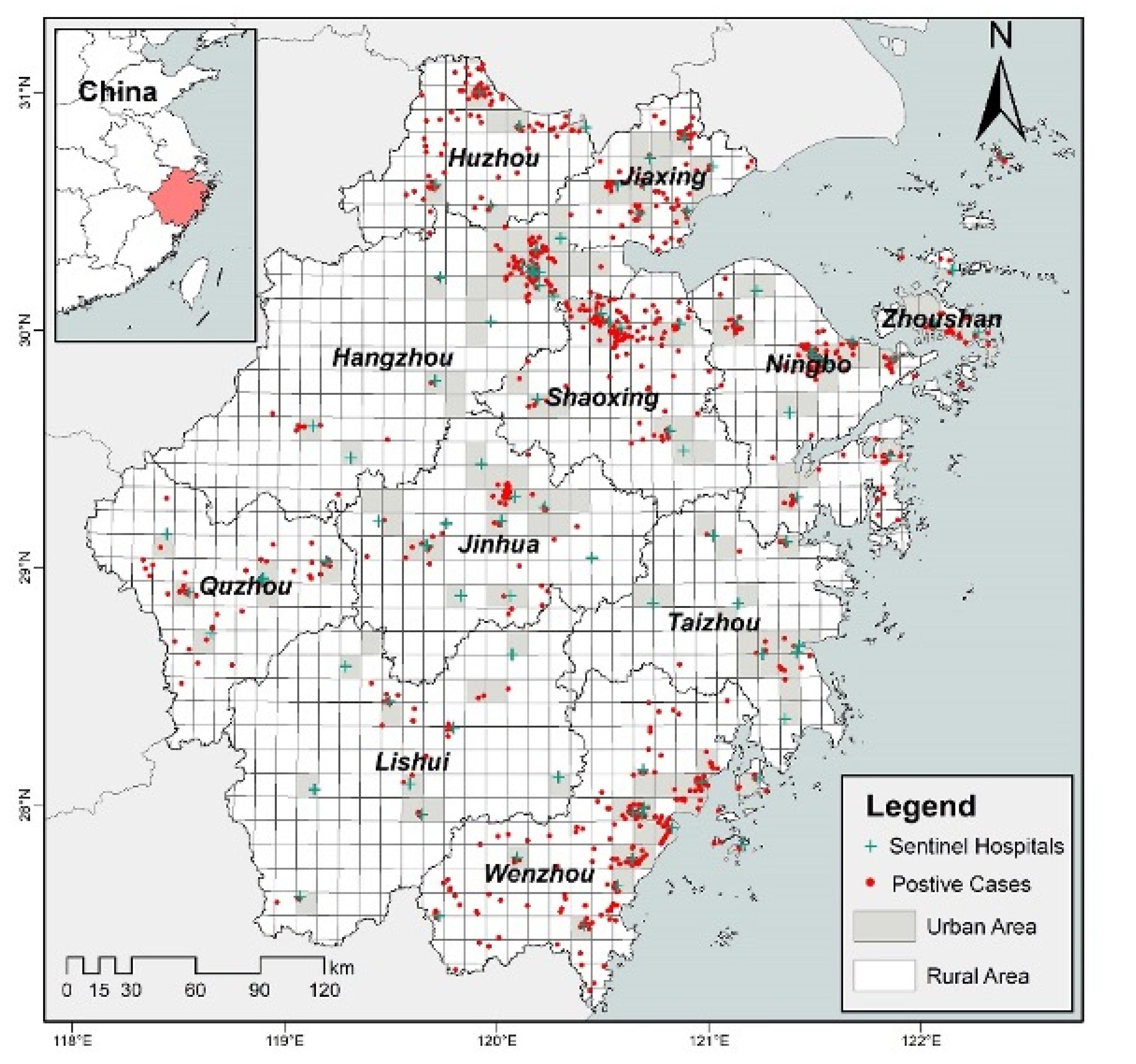
Figure 1. Locations of the study area (0.1° × 0.1° grid size) and positive cases caused by V. parahaemolyticus.
Remotesensing 14 03613 g001
Figure 2. Spatial distribution of variables and detection results of V. parahaemolyticus, including (a) wind speed, (b) dewpoint temperature, (c) temperature, (d) surface net solar radiation, (e) total precipitation, (f) daily maximum temperature, (g) daily minimum temperature, (h) road density, (i) proportion of construction area, (j) medical cost, (k) GDP, (l) population density, (m) NDVI, (n) distribution of urban and rural areas, and (o) test results.
Remotesensing 14 03613 g002
Figure 3. Spatial variation of regression coefficients in geographically weighted logistic regression model, including (a) temperature, (b) total precipitation, (c) road density, (d) dummy variable for rural areas, (e) proportion of construction area, and (f) GDP.
Remotesensing 14 03613 g003
Figure 4. Spatial variation of t-value in geographically weighted logistic regression model, including (a) temperature, (b) total precipitation, (c) road density, (d) dummy variable for rural areas, (e) proportion of construction area, and (f) GDP.
Remotesensing 14 03613 g004
Figure 5. Predicted risk map of foodborne disease cases caused by V. parahaemolyticus. (a) Global logistic regression model; (b) geographically weighted logistic regression model.
Remotesensing 14 03613 g005
Figure 6. Average of prediction probability within a certain distance and actual average detection rate. Note: The corresponding areas near the peak (A and B) are located in Jinhua and Quzhou, respectively.
Remotesensing 14 03613 g006
Table 1. Evaluation index system of foodborne diseases vulnerability.
CriterionIndexSourceResolutionYear
ExposureWind Speed (m/s)ERA5-Land
(https://www.ecmwf.int/ (accessed on 20 October 2021))
2018
Dewpoint Temperature (K)
Temperature (K)
Surface Net Solar Radiation (KJ/m2)0.1° × 0.1°
Total Precipitation (m)
Daily Maximum Temperature (K)
Daily Minimum Temperature (K)
SensitivityRoad Density (km/km2)Road Data
(https://www.openstreetmap.org/ (accessed on 23 March 2021))
Vector2021
Proportion of Construction Area (%)Land Use Data
(https://www.resdc.cn/ (accessed on 28 April 2021))
1 km2015
Rural AreasAdministrative Division Data (http://www.ngcc.cn/ngcc/ (accessed on 6 November 2021))Vector2018
Population Density (people/km2)Grid Population Density
(https://sedac.ciesin.columbia.edu/data/collection/gpw-v4 (accessed on 23 July 2022))
1 km2020
NDVIGrid NDVI
(https://www.resdc.cn/ (accessed on 28 April 2021))
1 km2018
AdaptabilityMedical Cost (h)POI from Amap
(https://restapi.amap.com/v3/place/text (accessed on 15 May 2013))
Vector2012
GDP (million yuan/km2)Grid GDP
(https://www.resdc.cn/ (accessed on 28 April 2021))
1 km2015
Table 2. Mean and standard deviations of urban and rural areas.
IndexTotalUrban AreaRural Area
964 Grids155 Grids809 Grids
Wind Speed (m/s)0.655 (0.405)0.767 (0.456)0.633 (0.391)
Dewpoint Temperature (K)286.204 (0.980)286.673 (0.792)286.114 (0.987)
Temperature (K)290.307 (0.892)290.788 (0.592)290.215 (0.911)
Surface Net Solar Radiation (KJ/m2)231,698.574 (8818.364)229,737.638 (9464.728)232,074.279 (8644.563)
Total Precipitation (m)0.052 (0.008)0.049 (0.006)0.053 (0.008)
Daily Maximum Temperature (K)294.143 (0.875)294.423 (0.830)294.089 (0.874)
Daily Minimum Temperature (K)287.010 (1.316)287.614 (1.150)286.894 (1.315)
Road Density (km/km2)3.105 (2.288)5.486 (3.544)2.649 (1.597)
Proportion of Construction Area (%)7.946 (11.614)22.643 (15.630)5.131 (8.052)
Population Density (people/km2)638.452 (1098.019)2048.545 (2105.047)407.526 (546.304)
NDVI0.783 (0.121)0.655 (0.130)0.807 (0.102)
Medical Cost (h)0.041 (0.063)0.017 (0.038)0.046 (0.065)
GDP (million yuan/km2)4762.486 (9651.622)10,687.459 (15866.161)3627.293 (7417.539)
Note: Standard deviations are in parentheses.
Table 3. Parameter estimates for the global logistic regression model.
VariableβS.Ez-ValuepExp(β)VIF
Temperature0.3900.1043.747<0.0011.4761.443
Total Precipitation0.2620.0992.6520.0081.3001.412
Road Density0.2720.1421.9140.0561.3121.820
Proportion of Construction Area0.3730.1223.0530.0021.4522.207
Is Rural Areas−0.9240.231−4.007<0.0010.3971.503
GDP0.5590.2122.6440.0081.7501.456
Intercept−1.2220.094−13.000<0.0010.295-
AICc952.390 Deviance938.390
AUC0.772
Table 4. Summary statistics for geographically weighted logistic regression parameter estimates.
VariableMeanSTDMinMax% −% +
Temperature0.4580.469−0.4911.69316.5%83.5%
Total Precipitation0.2970.637−0.8301.98237.4%62.6%
Road Density0.4611.076−1.7902.07232.4%67.6%
Proportion of Construction Area0.2730.506−0.7121.77729.0%71.0%
Is Rural Areas−1.3240.745−3.1870.38997.9%2.1%
GDP1.2181.768−6.4427.53512.5%87.5%
Intercept−0.0011.131−3.6974.11151.1%48.9%
AICc874.659 Deviance760.530
AUC0.871
Table 5. Percentage of foodborne disease risk areas and average prediction probability based on geographically weighted logistic regression model.
GradeTotal AreaUrban AreaRural Area
Very low (0–0.2)55.7%11.4%63.2%
Low (0.2–0.4)20.1%15.8%20.8%
Middle (0.4–0.6)12.3%17.1%11.5%
High (0.6–0.8)6.7%25.3%3.6%
Very High (0.8–1.0)5.2%30.4%0.9%
Average Prediction probability26.0%60.6%20.1%
Publisher’s Note: MDPI stays neutral with regard to jurisdictional claims in published maps and institutional affiliations.