1. Introduction
Since the concept of GNSS meteorology was first proposed by Bevis et al., the water vapor information derived from GNSS has drawn increasing attention in the meteorological and GNSS communities [
1]. The precipitable water vapor (PWV), which refers to the height of an equivalent column of water vapor [
2], has been widely validated to achieve mm-level accuracy based on the conversion of GNSS zenith tropospheric delay [
3]. Further, the three-dimensional water vapor information can also be inversed by using GPS signals as scanning rays in the research area, which is called water vapor tomography.
Braun et al. first proposed the concept of GPS water vapor tomography [
4] and Flores et al. first realized it using the data from the Kilauea network in Hawaii [
5]. The research region, covered by ground GPS receivers, is discretized into finite voxels according to its latitude, longitude, and altitude, and the unknown estimated parameter of the voxels are assumed to be constant during a given period. The GPS-derived slant water vapor is regarded as the observations for water vapor tomography.
In modeling the GPS water vapor tomography, it is found that the geometric distribution of the observed signals is an inverted cone due to the fixed structure of GPS sites and satellites [
6]. The direct effect caused by this phenomenon is the presence of tomographic voxels without signal rays passing through, especially at the lower and edge layer of the area of interest. It also makes many voxels be penetrated by only a very small number of signals. From the perspective of the water vapor tomography model, it often leads to a large number of zero elements appearing in the coefficient matrix, which becomes a sparse matrix [
7]. This is the fundamental cause of the ill-posed problem in GPS water vapor tomography, which seriously restricts its stable and high-accuracy solution. Obviously, enriching the observation equation of the GPS water vapor tomography is an effective way to overcome the above problem by introducing various observation information, and related research has been carried out.
Based on voxel horizontal boundary selection and non-uniform symmetrical division, Chen et al. and Yao et al. proposed an optimized approach of horizontal voxel division to introduce more signal rays penetrated from the top layer into the observation equation [
8,
9]. The similar effect can be obtained by the method of constructing the tomographic buffer area carried out by Trzcina et al. and Sa et al. [
10,
11]. These methods are limited to specific tomographic regions and certain experimental periods. Adavi et al. explored how to use the constructed virtual reference sites to augment location-specific GPS observations [
12]. The virtual signals were also introduced to the tomography model using the calculated mapping function and ZWD/PWV of corresponding site and the elevation and azimuth of specified virtual satellite [
6,
13]. Studies have shown that it is a feasible method to incorporate the GPS signal rays passed through form the side face into the tomography model; for example, Zhao et al. constructed the unit scale factor for these signals using the radiosonde and reanalysis data [
14], Zhang et al. and Hu et al. established the height factor models adapted to these signals from side face [
15,
16]. In addition, Zhao et al. tried to extend the observations of GPS sites outside the tomographic region into the tomography model based on the GPT2w and TMF models [
17,
18]. The above methods all rely on external data or models and tend to introduce new error for the observation information. On the other hand, some have attempted to add multi-source observation information from various sensors into the GPS tomography model, such as the COSMIC occultation data [
19], the GNSS-R data [
20], the InSAR data [
21,
22], WRF output data [
23], LEO constellation-augmented data [
24], PWV data derived from FY-3, and MODIS [
25,
26]. However, the spatiotemporal resolution, availability, and consistency with the tomographic region are the factors that seriously restrict the fusion of the above observations into the tomography model.
It is more reasonable and convenient to construct the GNSS water vapor tomography model together with the observations from GPS and the other three satellite navigation systems. Bender et al. simulated GPS, GLONASS, and Galileo data and introduced the method for obtaining three-dimensional water vapor information by tomography technique in multi-satellite systems [
27]. Wang et al. compared the tomographic accuracy of BDS and GPS based on simulated data, and showed that the result using 9 satellites of BDS is basically comparable to that of GPS [
28]. Xia et al. and Benevides et al. carried out the water vapor tomography experiments of GPS combined with GLONASS and GPS combined with Galileo in Hongkong and Lisbon regions, respectively [
29,
30]. Dong et al. and Zhao et al. utilized the measured data derived from different numbers of BDS2 satellites and combined it with GPS and GLONASS data to construct the tomography model in Wuhan and Guiyang, respectively [
31,
32]. With the gradual improvement of Galileo and the opening of BDS-3 services, the above experiments based on simulated data or incomplete satellite data cannot fully reflect the current status of water vapor tomography based on multi-GNSS. Therefore, this paper aims to explore the differences between the four satellite navigation systems and their combination in water vapor tomography, including the modeling process and the reconstructed results.
2. Materials and Methods
The observations in GNSS water vapor tomography are the slant water vapor (SWV) which can be converted from slant wet delay (SWD) as follows [
33]:
where
refers to the liquid water density with the unit of
;
denotes the universal gas constant;
and
represent the molar mass of water and the dry atmosphere and their values are
and 28.96
, respectively;
is the weighted mean temperature, which can be calculated by using surface temperature [
34,
35];
,
, and
are the empirical physical constants, which are equal to
,
, and
, respectively [
36]. After mapping the zenith wet delay (ZWD) and the wet delay gradients into the elevation direction, the SWD can be obtained as follows [
37]:
where
indicates the wet mapping function and the global mapping function (GMF) was used in this paper;
ele and
azi denote the satellite elevation and azimuth angles, respectively.
and
represent the wet delay gradient parameters in the east-west and north-south directions, respectively. Affected by water vapor along the signal ray, ZWD is the wet component of zenith total delay (ZTD) which is the primary parameter retrieved from GNSS observation. To obtain ZWD, the zenith hydrostatic delay (ZHD) should be subtracted from ZTD [
38]. In this paper, the Saastamoinen model is used to calculate the accurate ZHD using the pressure measurements as follows [
39]:
where
and
H denote the latitude and geodetic height of the GNSS site, respectively.
is the measured surface pressure.
In the water vapor tomography, the SWV value is also an integral expression of water vapor along the slant path from the ground receiver and GNSS satellite, given by the following:
where
in
denotes the water vapor density and
refers to the path traveled by a satellite signal ray. After discretizing the tomographic region into finite voxels, the observation equation of GNSS water vapor tomography can be established based on the distances of GNSS signal rays crossing the divided voxel and the unknown estimated water vapor density with each voxel. It can be expressed as follows:
where
n represents the total number of divided voxels in the research region.
denotes the distance of signal rays inside voxel
i, which can be calculated by using the coordinates of GNSS sites and satellites.
refers to the water vapor density of voxel
i, which is the unknown estimated parameter.
In water vapor tomography, two types of constraints are widely used in tomographic modeling along with the observation equation, one is the horizontal constraint and the other is vertical constraint, since a spatial relation exists between water vapor in a specific voxel and its surrounding ones. For the horizontal constraint, it assumes that the distribution of water vapor density is relatively stable in the horizontal direction within a small region, and represents the relationship between the water vapor density of a certain voxel and those of its adjacent voxels in the same layer. For the vertical constraint, it refers to the exponential relationship between the water vapor density of voxels for two consecutive layers. These two constraints can be expressed as follows:
where
m is the total number of voxels in the same layer.
and
denote the horizontal weighted coefficient and the vertical weighted coefficient, respectively. The horizontal weighted coefficient is constructed based on the Gaussian inverse distance weighted function as the following equation:
where
d is the distance between the two voxels.
j is a number from 1 to
m, represented the voxel ordering of the same horizontal layer.
denotes the smoothing factor. The vertical weighted coefficient is constructed based on exponential function as follows:
where
h represents the height of the corresponding voxel and
Hs refers to the water vapor scale height with an empirical value of 1.5 km [
40]. Note that each voxel has corresponding equations for horizontal and vertical constraints.
Thus, the tomography model for water vapor reconstruction can be established by combining the observation equation of multi-GNSS and the two types of constraint equations.
where
denotes the vector with SWV values derived from these four satellite systems;
A represents the coefficient matrices of the observation equation for different types of satellite systems;
H and
V are the coefficient matrices of the horizontal and vertical constraints, respectively. The tomography solution of the unknown water vapor density vector
x can be obtained as follows:
where
P represents the weighting matrices of different equations, which are determined by an optimal weighting method using the variance components estimation and homogeneity test [
41]. Note that the number of satellite systems in Equations (8) and (9) can be adjusted in the experiment.
3. Results
3.1. Experimental Description
In this paper, the Hong Kong satellite Positioning Reference Station Network (SatRef) was selected to conduct the water vapor tomography experiment. We divided this research region into 560 voxels ranging from 113.87° to 114.35°, from 22.19° to 22.54°, and from 0 to 8 km for longitude, latitude, and altitude, respectively; that is, a voxel of 8 × 7 in the horizontal direction and 10 layers in the vertical direction. As shown in
Figure 1, thirteen GNSS sites (T430, HKKT, HKLT, HKSL, HKNP, HKMW, HKPC, HKLM, HKOH, HKSC, HKST, HKSS, HKWS) in this region were used to provide SWV in the tomography modeling, and one GNSS (HKQT) and one radiosonde (45004) site were selected to validate the results of the water vapor tomography.
We utilized the GAMIT 10.71 software to estimate the tropospheric parameters including ZTD and gradient parameters using the four GNSS systems. In this process, the elevation cutoff angle was set to 15°, the IGS precise ephemeris was adopted. Three MEGX stations (JFNG, URUM, and LHAZ) were incorporated into the solution model to reduce the strong correlation of tropospheric parameters caused by the short baseline. The processing strategies were set to LC_AUTCLN and BASELINE modes, meaning that the ionosphere-free linear combination was selected and the orbital parameters were fixed, respectively. The tropospheric parameters, including troposphere delay gradients and ZTD at 4 and 2 h intervals, are estimated and interpolated to a 30 s sampling rate in the GAMIT software. After calculating the ZHD using the measured pressure recorded by an automatic meteorological device, the SWV values of each satellite system were obtained by using Equations (1) and (2).
In this experiment, the GNSS observation data of one month from DOY 121 to 151, 2021 were selected to conduct the modeling and solution of water vapor tomography. For each tomographic solution, the period covered is 0.5 h. To assess the performance of water vapor tomography based on different satellite systems and different combinations of satellite system, each tomographic solution has 15 results, including those of a signal satellite system, the combination of two satellite systems, the combination of three satellite systems, and the combination of four satellite systems, namely GPS (G), BDS (C), GLONASS (R), Galileo (E), GPS+BDS (GC), GPS+GLONASS (GR), GPS+Galileo (GE), BDS+GLONASS (CR), BDS+Galileo (CE), GLONASS+Galileo (RE), GPS+BDS+GLONASS (GCR), GPS+BDS+Galileo (GCE), GPS+GLONASS+Galileo (GRE), BDS+GLONASS+Galileo (CRE), and GPS+BDS+GLONASS+Galileo (GCRE). Note that both BDS-2 and BDS-3 were included in the experiment.
3.2. Experimental Analysis
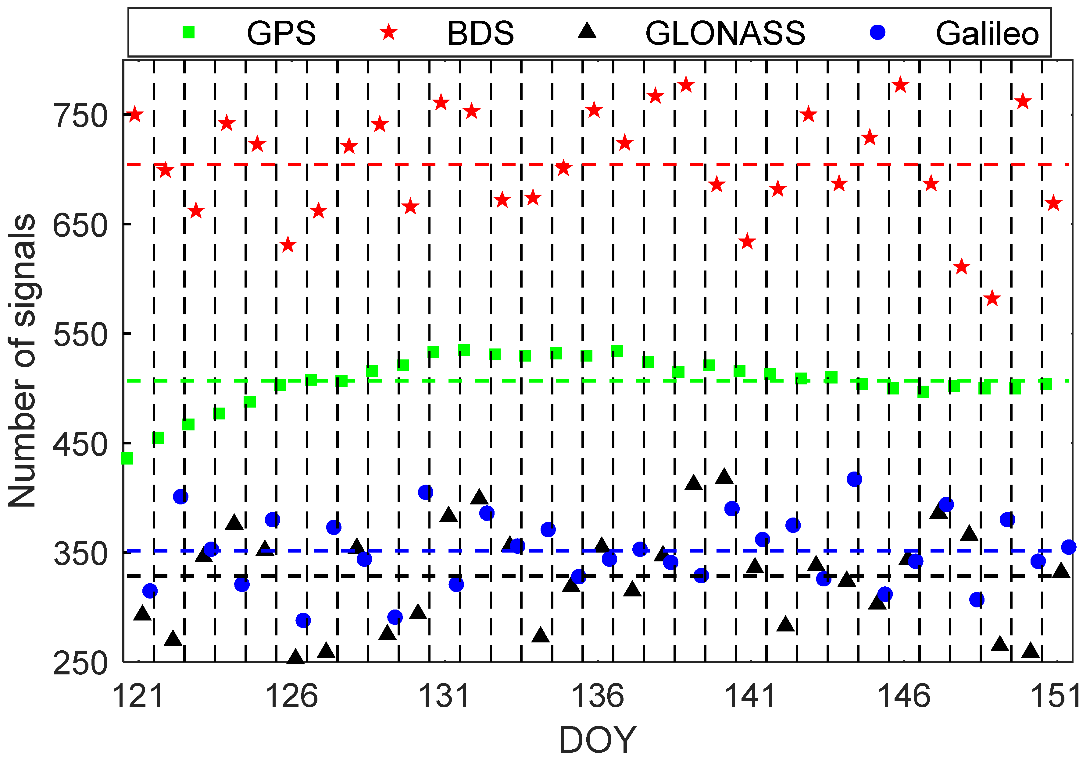
The number of satellite signal rays available for the four satellite systems in each tomographic solution is counted and their averages during the 31 days from DOY 121 to 151, 2021 are shown in
Figure 2. It can be seen that the BDS has the largest number (704) of available signal rays, followed by GPS, Galileo, and GLONASS with the average values of 507, 329, and 351, respectively. The percentages of available signal rays in BDS that exceed GLONAA and Galileo are more than 100%, achieving 114% and 101%, respectively. Compared with GPS, the value also reaches 39%. The number of signal rays used in GPS is the most stable during the experimental period, the difference between the maximum and minimum value is less than 100 with the standard deviation (STD) being only 23. While the other three satellite systems have obvious fluctuations in the number of available signal rays, with the differences between the maximum and minimum value far greater than 100 and the STDs reach 51, 48, and 34 for BDS, GLONASS, and Galileo, respectively. Note that the average number of signal rays used in Galileo is greater than that of GLONASS, but there are still days when GLONASS has more available signal rays than Galileo. When the satellite systems are combined, only the available signal rays of RE have just reached the level of BDS and the other combinations are all obviously improved compared with these single systems, especially since the average number of signal rays used in the combination of four systems could be close to 2000.
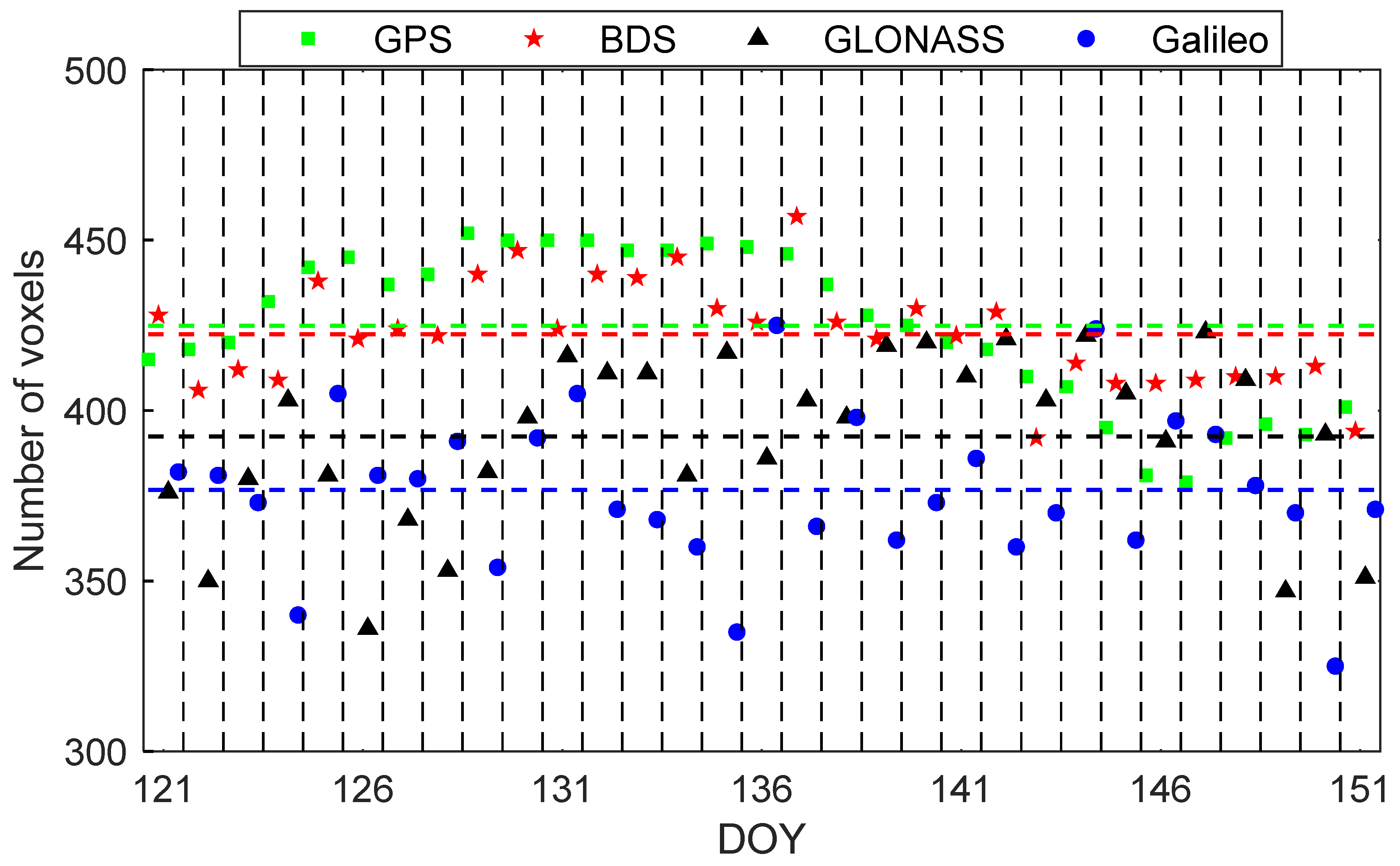
The number of voxels passed through by signal rays for the four satellite systems in each tomographic solution is also counted, and their average values are shown in
Figure 3. It was observed that the GPS has the largest number of voxels crossed by signal rays, followed by BDS, GLONASS, and Galileo with average values of 425, 424, 392, and 377, respectively. Corresponding to the 560 voxels in the entire tomographic region, the coverage rate of the four satellite systems reaches 75.9%, 75.4%, 70%, and 67.3%, respectively. Note that GPS and GLONASS with fewer available signal rays have more penetrated voxels than BDS and Galileo, respectively, and in fact, their differences are relatively small. In addition, the number of voxels crossed by signal rays for the four satellite systems all show a certain fluctuation during the experimental period.
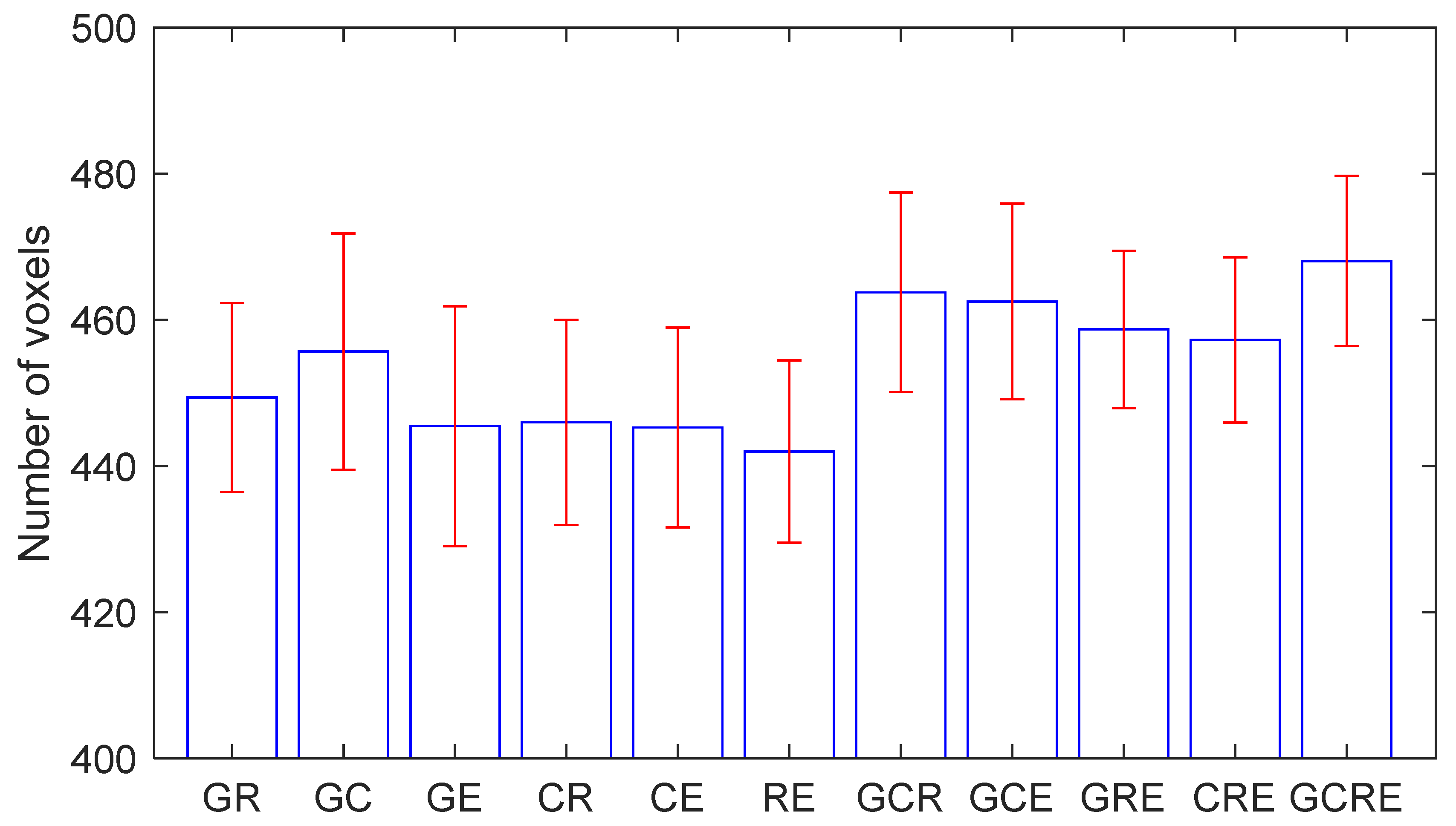
When combining the satellite systems, the number of crossed voxels and their coverage rate is counted and shown in the form of a histogram in
Figure 4. It can be seen that the number and coverage rate of voxels are increased after the combinations compared with single satellite system. In addition, the performances of the three-satellite systems combination are better than those of the two-satellite systems combination, and four satellite systems combination outperforms the three-satellite systems combination. Specifically, combination of GCRE achieved the best performance with the number and coverage rate of voxels of 468 and 83.6%, respectively.
In the tomographic experiment, we found the existence of voxels that were only penetrated by a few signal rays, thus the concept of voxels crossed by sufficient signal rays was introduced from the relevant literature [
7]. Based on the fact that a ray crossed a minimum number of voxels when the signal ray passed vertically through the tomographic region, the minimum probability that a voxel will be penetrated by a ray could be calculated. In this experiment, the value is 10/560, namely 1.79%. Then, the value of minimum probability multiplied by total SWV used is regarded as the criteria to determine whether a voxel is crossed by sufficient signal rays. Therefore, the number of voxels passed through by sufficient signal rays for the four single satellite systems and their combinations are counted and listed in
Table 1 during the experimental period. It was observed that GPS had the largest number of voxels penetrated by sufficient signal rays among the four single systems, and only 7 voxels more than Galileo with the least effective voxels. After the combinations, the number of voxels increased but very little and the value of the combination of four system was only 278. Regarding the coverage rate, the difference of those 15 values in
Table 1 is even smaller.
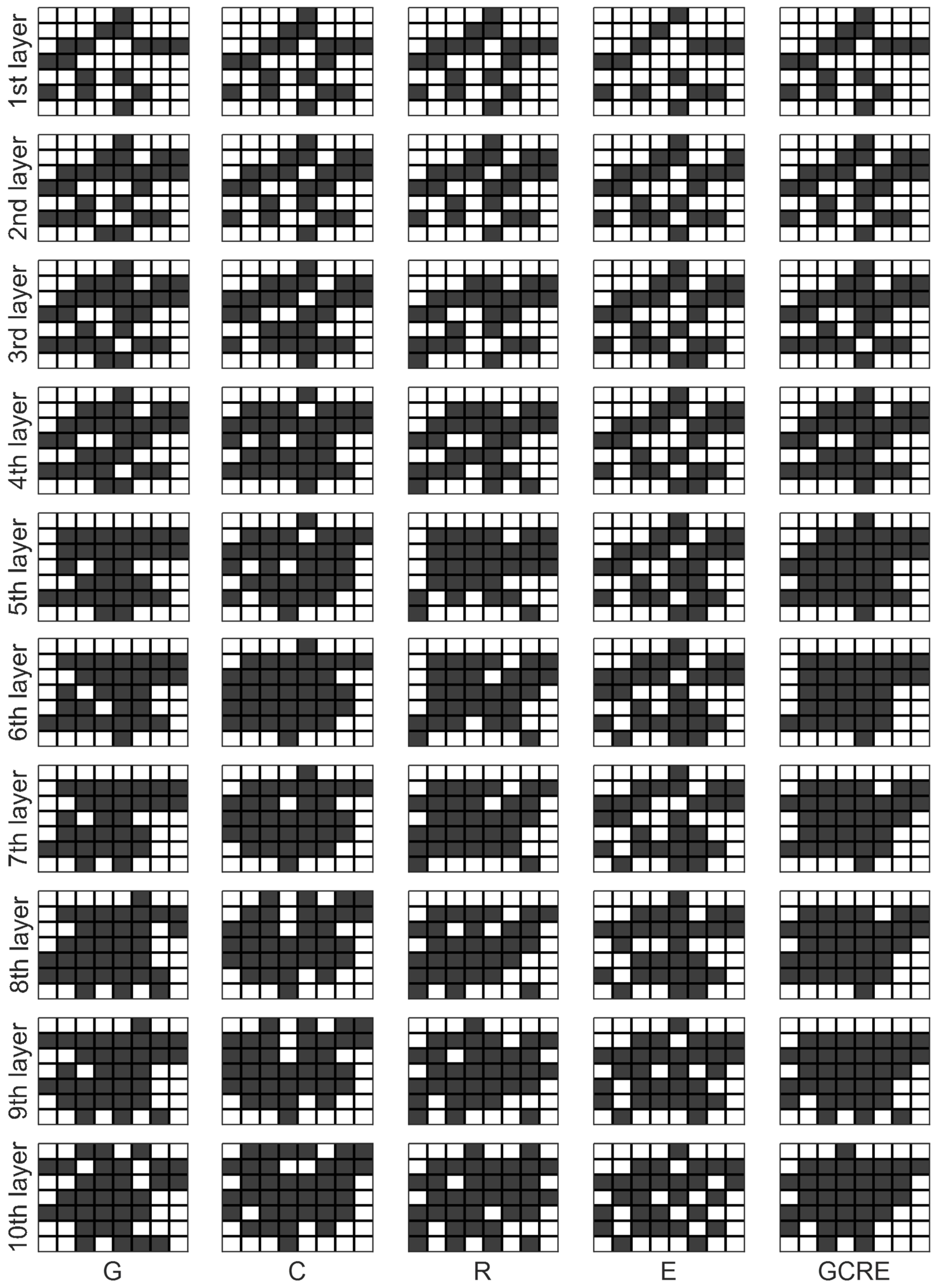
Further, the situation that each voxel passed through by signal rays in a certain tomographic solution (UTC 11:45–12:15, DOY 137, 2021) is shown in detail in
Figure 5, in which the black and white rectangles represent the voxels crossed by sufficient and in sufficient signal rays, respectively. Note that only the four single satellite systems and the combination of the four systems are illustrated in this figure. It is observed in the figure that the distribution of the black and white rectangles for different systems is very similar, especially in the lower and middle layers. From this point, for water vapor tomography in Hong Kong, the selection of a single satellite system or multi-GNSS combination has little effect on the structure of the tomographic model.
4. Discussion
To assess the performance of water vapor tomography using different satellite systems, SWV of the GNSS sites for validation were computed using these 15 tomographic results and the distances of signal ray in each voxel based on the observation equation established in Equation (5). The 15 tomography-computed SWV were then compared with the GAMIT-estimated SWV (as a reference).
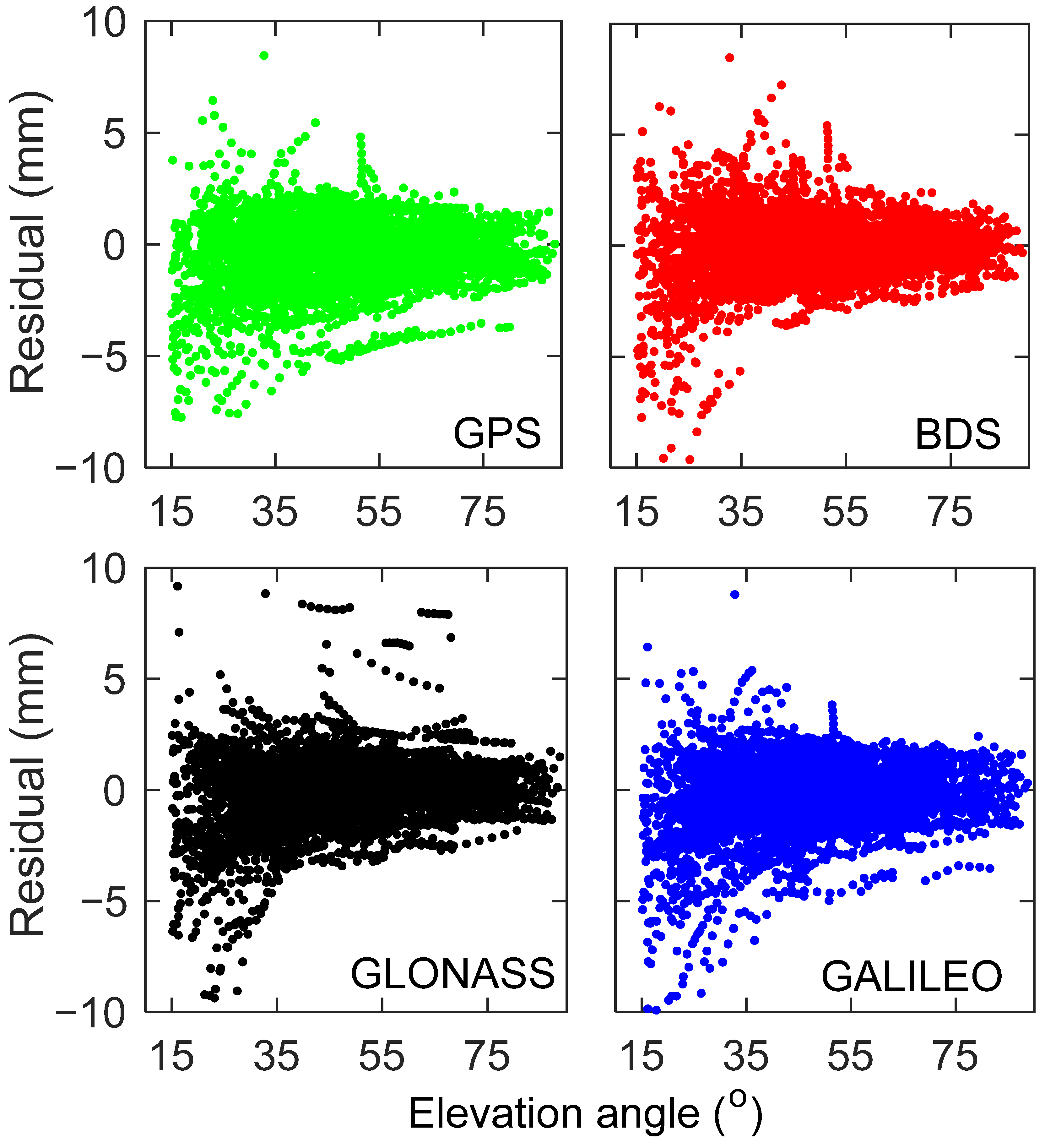
Figure 6 shows the change of tomography-computed vs. GAMIT-estimated SWV residuals with elevation angle during the experimental period for the four single systems. The change of the SWV residuals has the same trend in the four satellite systems, and they decrease as the elevation angle increases. It is observed that the residuals of four systems all ranged from −10 to 10 mm, and most of them concentrated between −2.0 and 2.0 mm. The percentage of absolute residuals smaller than 2.0 mm are 86.9%, 88.1%, 85.7%, and 85.3% for GPS, BDS, GLONASS, and Galileo, respectively. The largest absolute residual of the four satellite systems is 8.46, 9.63, 9.37, and 9.91 mm, respectively. We obtained the SWV residuals for various combinations of satellite systems, which also follow a decreasing trend with increasing elevation. These ranges and concentrated areas of the SWV residuals are unchanged compared with the four single satellite systems.
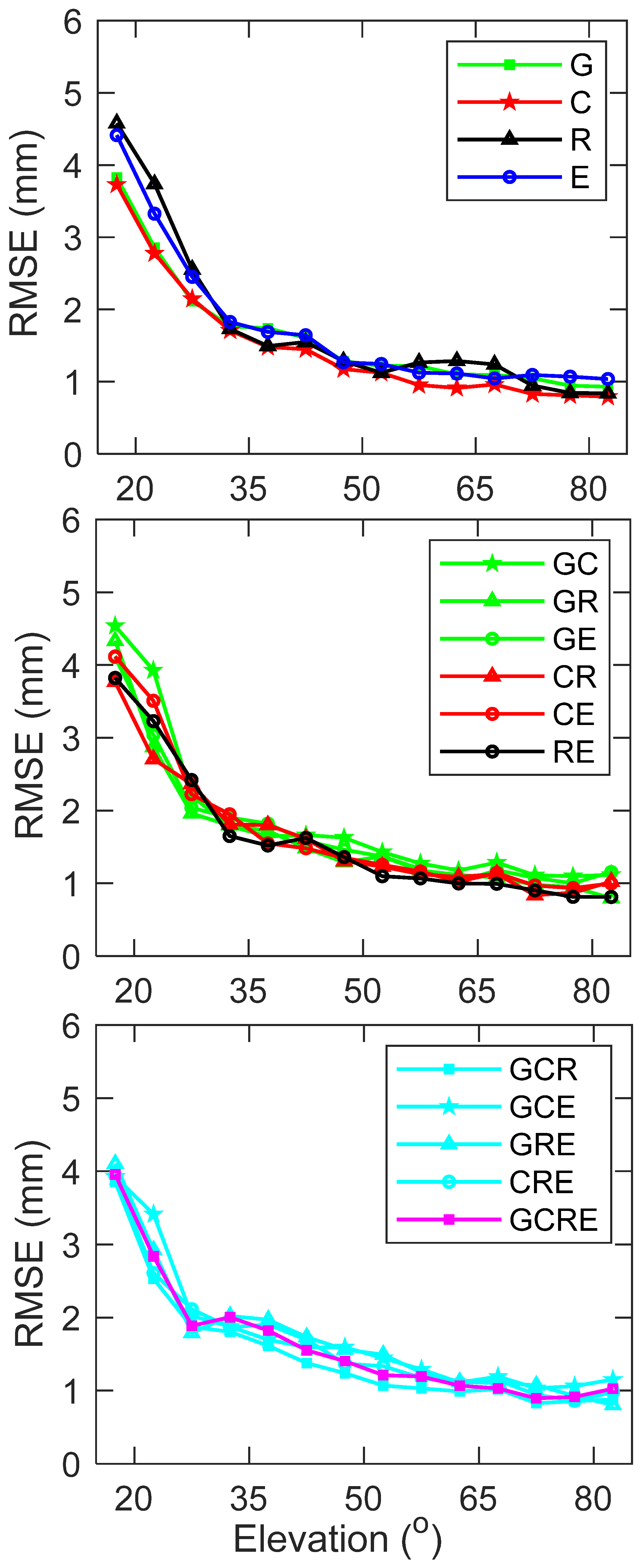
To further assess their performance, SWV values were grouped into individual elevation bins of 5°, i.e., all SWVs with an elevation angle between 15 and 20° were evaluated as a single unit. Thus, the RMSE of each elevation bin for these 15 tomographic results was calculated and is shown in
Figure 7. It can be seen from the left panel that the GLONASS and Galileo performance is not as good as the BDS and GPS at low elevation angles. As the elevation angle increases, their differences become very small. BDS achieved the best RMSE with a value of 1.59 mm, followed by GPS, Galileo, and GLONASS. In fact, the differences between these RMSEs are small and the values do not exceed 0.2 mm. Considering the magnitude range of SWV, these differences can be negligible. After the combinations, the RMSE of SWV residuals in each elevation bin were shown in the middle and right panels, which are the combination of two systems and multi systems, respectively. The RMSE difference of the SWV residuals for various combinations is relatively small in each elevation bin. Specifically, the RMSEs of whole SWV residuals are 1.66, 1.59, 1.75, 1.74, 1.68, 1.64, 1.67, 1.62, 1.63, 1.60, 1.59, 1.64, 1.65, 1.65, and 1.63 mm for G, C, R, E, GC, GR, GE, CR, CE, RE, GCR, GCE, GRE, CRE, and GCRE, respectively. Considering the magnitude range of SWV values, the differences of RMSE mentioned above not more than 0.2 mm could be negligible. Therefore, it is concluded that the tomographic results of different satellite systems and different combinations have little difference in SWV validation.
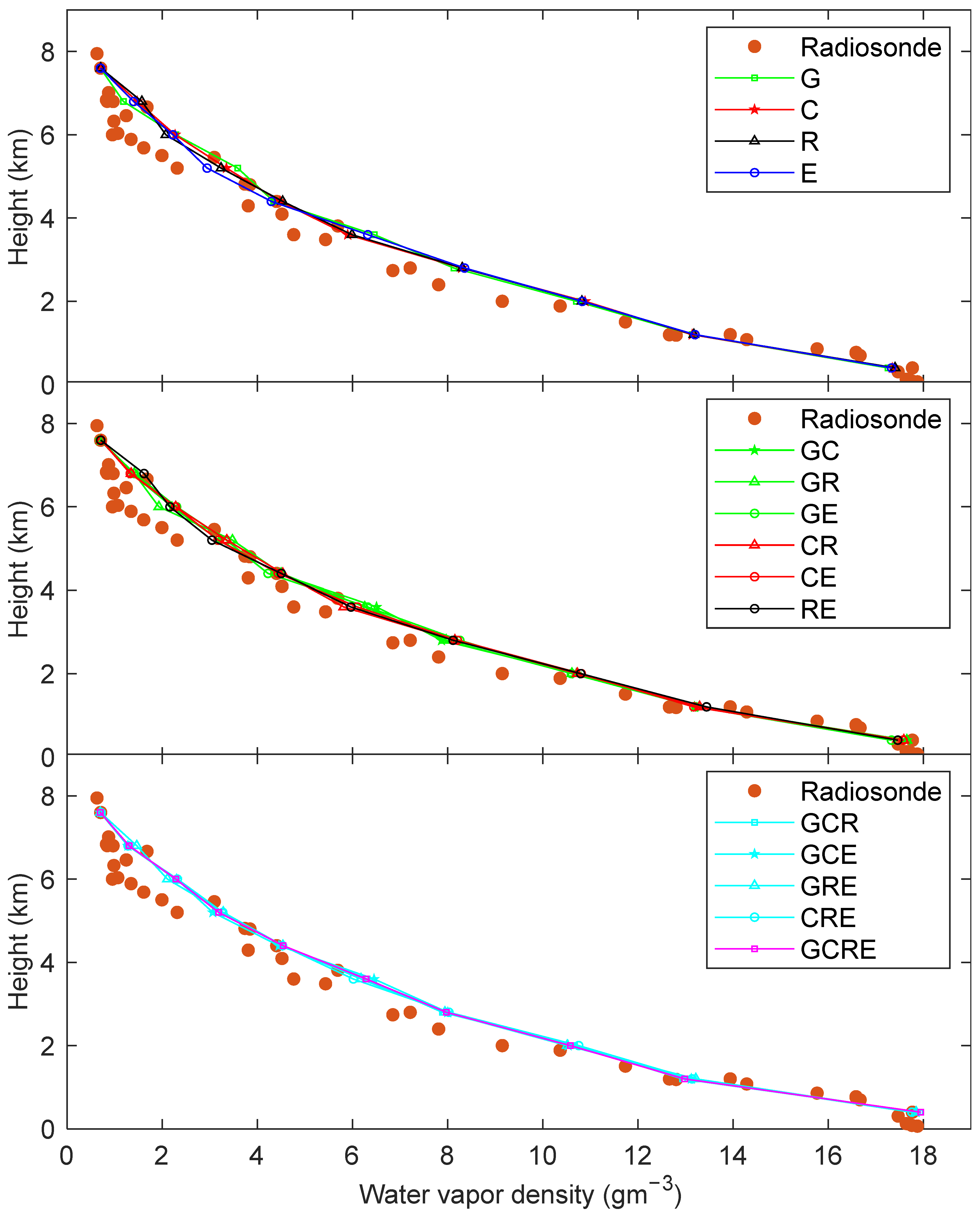
Radiosonde data are well suited as a reference to validate the accuracy of the water vapor tomography results, since they can provide a water vapor density profile with high precision based on the atmospheric parameters obtained at different altitudes.
Figure 8 illustrates the water vapor density comparisons between radiosonde data and these 15 tomographic results for different altitudes on UTC 11:45–12:15, DOY 137, 2021, which is consistent with the time of tomographic solution shown in
Figure 5. It is clear from the profiles that the water vapor density decreased with increasing height. The water vapor density profiles reconstructed by these 15 tomographic results conform with those derived from radiosonde data. From
Figure 8, it is difficult to observe the difference in the water vapor density reconstructed by different satellite combinations. Therefore, the radiosonde comparison of 31 days from DOY 121 to 151, 2021 was conducted and the statistical results were listed in
Table 2 to further illustrate their performances. From the mean value of RMSE, the difference between the WVD results reconstructed by single system tomography is 0.05 gm
−3, and BDS and GPS outperforms GLONASS and Galileo slightly. Compared with the single system, improvement can be observed from the WVD results reconstructed after the satellite system combination. The largest improvement appears from the Galileo with a RMSE of 1.46 gm
−3 to the combination of GCR with a RMSE of 1.30 gm
−3. The number of satellite systems in the combination (two, three, or four satellite systems) did not present an obvious impact on the WVD results reconstructed by water vapor tomography.
5. Conclusions
In this paper, the performances of the four navigation satellite systems and their combinations in the water vapor tomography were analyzed and assessed using the GNSS data of SatRef in Hong Kong. In the tomographic modeling, the signal rays that can be used, the voxels crossed by signal rays, and the number and distribution of the effective voxels were computed and counted for these different combinations. For the tomographic results, the GAMIT-estimated SWV of HKQT and the water vapor density derived from radiosonde were selected as references to assess these 15 tomographic solutions.
In the experimental period, the average number of available signal rays was 507, 704, 329, and 351 for GPS, BDS, GLONASS, and Galileo, respectively. Combining satellite systems in water vapor tomography can increase the number of available signal rays, especially as the value of four-system combination reaches close to 2000. The average number of voxels crossed by signal rays are 425, 424, 392, and 377 for GPS, BDS, GLONASS, and Galileo, respectively, showing that the number of penetrated voxels is not entirely determined by the number of available signal rays. The combinations improved the number of voxels crossed by signal rays; for example, the number and coverage rate of penetrated voxels achieved by GCRE are 468 and 83.6%, respectively. When the voxels with sufficient signal rays are concerned, these 15 tomographic solutions differ very little in both number and coverage rate. The distribution diagram of effective voxels based on black and white rectangle also indicated the small differences in the 15 solutions. The numerical statistics showed that the RMSE in SWV comparison are 1.66, 1.59, 1.75, 1.74, 1.68, 1.64, 1.67, 1.62, 1.63, 1.60, 1.59, 1.64, 1.65, 1.65, and 1.63 mm for G, C, R, E, GC, GR, GE, CR, CE, RE, GCR, GCE, GRE, CRE, and GCRE, respectively. In the comparison with radiosonde data, the average RMSE are 1.42, 1.41, 1.45, 1.46, 1.33, 1.34, 1.41, 1.34, 1.36, 1.40, 1.30, 1.34, 1.36, 1.37, and 1.32 gm−3 for these 15 tomographic results. The above comparisons indicated that the differences in the tomographic results of a single satellite system are small, and the combinations of satellite systems have limited improvement in the water vapor tomography results.
In the follow-up research, the impact of different satellite systems and their combination on water vapor tomography need to be explored in more representative regions. In addition, the number, distribution, and density of GNSS stations in the research region is another important factor determining the structure of the tomographic model. Thus, it is necessary to pay more attention to the influence of the GNSS sites on water vapor tomographic results in the case of a determined satellite system.


