Technical Note

High-Throughput Remote Sensing of Vertical Green Living Walls (VGWs) in Workplaces

1
Department of Soil & Water Sciences, Institute of Environmental Sciences, The Robert H. Smith Faculty of Agriculture, Food and Environment, The Hebrew University of Jerusalem, Rehovot 7610001, Israel
2
The Advanced School for Environmental Studies, The Hebrew University of Jerusalem, Jerusalem 9112102, Israel
*
Author to whom correspondence should be addressed.
Remote Sens. 2022, 14(14), 3485; https://doi.org/10.3390/rs14143485
Submission received: 22 June 2022 / Revised: 15 July 2022 / Accepted: 19 July 2022 / Published: 21 July 2022
(This article belongs to the Special Issue Urban Vegetation and Ecology Monitoring Using Remote Sensing)

Abstract

:
Vertical green living walls (VGWs)—growing plants on vertical walls inside or outside buildings—have been suggested as a nature-based solution to improve air quality and comfort in modern cities. However, as with other greenery systems (e.g., agriculture), managing VGW systems requires adequate temporal and spatial monitoring of the plants as well as the surrounding environment. Remote sensing cameras and small, low-cost sensors have become increasingly valuable for conventional vegetation monitoring; nevertheless, they have rarely been used in VGWs. In this descriptive paper, we present a first-of-its-kind remote sensing high-throughput monitoring system in a VGW workplace. The system includes low- and high-cost sensors, thermal and hyperspectral remote sensing cameras, and in situ gas-exchange measurements. In addition, air temperature, relative humidity, and carbon dioxide concentrations are constantly monitored in the operating workplace room (scientific computer lab) where the VGW is established, while data are continuously streamed online to an analytical and visualization web application. Artificial Intelligence is used to automatically monitor changes across the living wall. Preliminary results of our unique monitoring system are presented under actual working room conditions while discussing future directions and potential applications of such a high-throughput remote sensing VGW system.

Graphical Abstract

1. Vertical Green Living Walls (VGWs) as an Urban Nature-Based Solution (NBS)

Nature-based solutions (NBSs) refer to efforts aimed at tackling socio-environmental challenges by the use of nature through sustainable management. As part of NBS, the concept of “green” cities has been recommended for sustainable urban development [1,2]. The idea is to introduce vegetation into spaces within the urban fabric to reduce the heat island effect and air pollution in the city [3]. Such a solution could also support efforts to achieve carbon-neutral cities since plants uptake CO2 from the environment. The European Commission has proposed such a solution, which was recently adopted by Horizon 2030 as one of the potential strategies to meet the goal of carbon-free cities [4].
Since introducing new parks and gardens in the urban fabric is not straightforward, as free spaces are rarely found in modern cities, deploying vertical greening systems may be the optimal solution. Introducing vertical green systems into the city where the vegetation is grown on new or existing vertical walls has great potential as an NBS. These vertical green living systems (VGSs) are presently found in indoor and outdoor environments through a plethora of growing techniques [5,6,7]. However, the main challenge of such NBSs is understanding how these VGSs respond to and affect the urban environment. Another challenge is the management of such systems, which requires a different approach than the conventional management of horizontal green systems.
Since the VGS term also includes vertical growing in horizontal layers (one layer on top of the other), where the plants grow in the vertical direction, in this paper, we distinguish such systems from systems that grow vegetation on a vertical wall, where plants grow mostly in the horizontal direction (Figure 1a). We name such systems as vertical green wall (VGW) systems and use this term throughout this paper.
While extensive research exists on the effects of cooling [8] and humidity regulation [9,10], as well as the reduction in air pollutants [11,12,13], carbon dioxide [14], and particulate matter [15,16], of both indoor and outdoor VGSs and VGWs, most of the studies are focused on conventional horizontal planting systems and traditional potted plants. Since the vertical living wall approaches are a recent innovation, little is known about the potential impacts of such new horticultural living walls, known as VGW systems, on indoor air quality and comfort [17]. The increased plant density of VGW systems, vertical alignment, and higher areal and microflora exposure likely have distinct environmental impacts compared with the traditional potted systems [18,19].
The little-known fact about these systems through the few existing studies is that indoor VGW systems can reduce formaldehyde [20] and efficiently filter indoor particulate matter [11]. Recent studies also showed that VGW systems can reduce indoor carbon dioxide [14]. However, most of these studies are held in small cells or tiny room spaces under controlled conditions. High levels of indoor carbon dioxide are known to affect working performance. For example, research conducted at the Harvard T.H. Chan School of Public Health showed that office workers increased their cognitive performance when exposed to a more ventilated room with lower carbon dioxide levels [21]. Thus, indoor VGWs can potentially improve indoor air quality in workplaces, providing the required environment for better working conditions. However, a major challenge remains the spatiotemporally continuous monitoring of the performance of the VGW and its effect on the surrounding environment.

2. Using Remote-Sensing-Based Precision Agriculture Tools in VGWs

In terms of effect, the spatial dimension of the VGW system is crucial. To provide recommendations regarding the total area of the VGW system needed to reduce carbon dioxide in a room with a specific volume, for example, it is necessary to assess its spatial effect, which includes knowing the response at a given planting density as well as the plant type response to ambient and elevated CO2 conditions. While most studies explore the effects of living systems by measuring air quality in the room, how different wall parts react to their surrounding environment is still unknown. This effect may further change across the wall and through time. The same plant, for example, may respond differently due to its position in the wall because of the different exposure to local environmental conditions (e.g., light, ventilation, water supply, etc.). This spatial information is required to monitor and manage such systems properly.
Today, VGWs are expected to be automatically or semi-automatically maintained to become efficient systems. In that sense, proximal sensing, using cameras that measure the spectral and thermal signals reflected and emitted by the plants on the wall, can be leveraged to monitor variations across the VGW as well as to effectively manage such systems through smart decision support systems. Using proximal and remote sensing to track the performance of VGWs in carbon dioxide and temperature reduction capacity while associating spatial changes across the wall to variations in indoor environmental conditions is a promising management solution for these innovative NBS systems [22].
The general idea is to deploy precision agriculture techniques developed and used in conventional farming (horizontal vegetation systems) in VGW systems. For example, the photochemical reflectance index (PRI), which is based on spectral data acquired from proximal or remote sensing, was found to be associated with volatile organic compounds [23], as well as photosynthetic traits [24,25]. Thus, using spectral images of the proper wavelength bands may allow the generation of the wall’s PRI maps through time. This information may be beneficial to monitoring changes in CO2 uptake across the wall, helping automatically or semi-automatically manage the VGW system and improving its efficacy in reducing indoor carbon dioxide concentrations. Models driven by spectral-based vegetation indices [26,27,28] can be used to provide a spatial assessment of the plants’ water use and carbon uptake rates across the VGW. Thermal information, commonly used to assess water stress conditions in crops and trees [29,30,31], may also be used to determine transpiration rates across the VGW system for irrigation control purposes.
This short descriptive paper presents a first-of-its-kind high-throughput monitoring system of an indoor VGW that includes low- and high-cost sensors, thermal and hyperspectral remote sensing, and in situ gas-exchange measurements. In addition, air temperature, relative humidity, and carbon dioxide concentrations are constantly monitored in an operating workplace room (scientific computer lab) where the VGW is established, while data are continuously streamed online to an analytical and visualization web application. We show preliminary results of our monitoring system under actual working room conditions, discussing future directions and potential applications of such a sensing high-throughput monitoring VGW system.

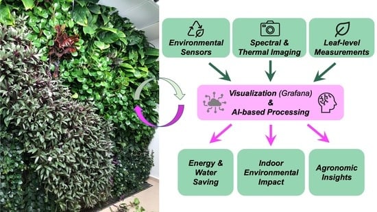
3. Description and First Results of the High-Throughput VGW Monitoring System

3.1. The VGW System in the Modeling and Monitoring Vegetation Systems Lab

A 15 m2 VGW system was established on April 2021 in the Modeling and Monitoring Vegetation Systems lab (M&M-VS; http://davidhelman.weebly.com) at the Faculty of Agriculture, Food and Environment, in Rehovot, Israel (Figure 1a). The VGW is a hydroponic system based on Patrick Blanc’s method in which the vegetation is directly transplanted into several layers of clothing, which are adhered to the wall [32]. Irrigation is applied daily (7 am) from the top of the wall via a computer-based drip irrigation system. Water is collected at the bottom through a drainage system that streams the water back to a 200 L tank placed behind the wall in a separate room (Figure 2). The water is pumped again from the tank the following day after filling to 130 L at the end of the previous day. The tank is completely emptied and refilled with fresh water and fertilizer on Tuesdays. Sensors in the tank continuously monitor pH and salinity (electrical conductivity, EC) every 10 s. The pH of the water is maintained at 6–7 and the EC at 1.4–1.6 mS cm−1.
The water is enriched with a “Bounty1” fertilizer (Zalmanson Fertilizers ©) to a 4:2:6 NPK composition. In addition, 0.75% calcium, 0.9% magnesium, and 6% microelements in chelation are added to the water to reach a total concentration of 2 mL L−1. The average daily water consumption of the wall is 16.5 ± 6.4 L day−1.
Artificial light in the photosynthetic range (wavelength of 400–700 nanometer) is the only energy source for the plants on the VGW in the room. However, light conditions are not homogeneous across the wall, with light intensities ranging from 10 μmol photons m−2 s−1 to 190 μmol photons m−2 s−1, which allows us to examine the species’ response under different light conditions (Figure 1b).
Six main species were planted across the 15 m2 VGW system (Figure 1a), with an average distance of 20–30 cm between the plants. In what follows, a short description of the six species is provided. Table 1 summarizes the main traits of each species.

3.1.1. Peperomia obtusifolia

Usually called “baby rubber plant”, “American rubber plant”, or “pepper face”, this plant has relatively smooth and thick round leaves. Peperomia is native to Mexico, South America, and West Indies. The plant can reach a height of 30 cm. It prefers bright indirect light conditions. Ideal temperatures for this species range from 16 °C to 26 °C, and pH from 6 to 8 [33]. According to the American Society for the Prevention of Cruelty to Animals, P. obtusifolia is non-toxic for humans and animals [34].

3.1.2. Tradescantia spathacea

Also known as “Moses in the cradle”, “boat lily”, and “wandering jew”, this plant is native to tropical areas such as Belize, Guatemala, and southern Mexico. It can be an understory plant in coastal forests, shrublands, pinelands, hammocks, secondary forests, cultivated grounds, and disturbed areas from sea level to low elevations [35]. T. spathacea may reach a maximum height of 30–50 cm. It is a very fast-growing species, easy to maintain. T. spathacea preferred conditions are warm and humid, with temperatures ranging from 14 °C to 27 °C [36]. It can be found in indoor and outdoor growing systems. T. spathacea can be toxic to animals and humans [37].

3.1.3. Chlorophytum comosum

Usually known as the “spider plant”, this is a perennial flowering plant native to tropical and southern Africa but was introduced to other parts of the world, such as western Australia [38]. It is easy to grow as a houseplant, prospering under various environmental conditions. C. comosum is well-known for its medicinal characteristics [38]. The ideal temperatures in which this species grow and develop range from 15 °C to 30 °C, with pH recommended levels of 6 to 6.5. C. comosum was found by the NASA Clean Air Study to effectively remove common household air toxins such as formaldehyde and xylene [39]. It is not toxic to animals and humans [34].

3.1.4. Spathiphyllum wallisii

Usually called “peace lily”, it is a genus of more than 47 species of monocotyledonous flowering plants from the Araceae family, which are very popular as indoor house plants. This species is native to tropical regions of the Americas and southeastern Asia. The evergreen herbaceous perennial plants have large leaves of 12–65 cm long and 3–25 cm broad. The flowers are produced in a spadix, surrounded by a white, yellowish, or greenish spathe. Spathiphyllum requires relatively small amounts of light and water. It is also known to remove household air toxins such as benzene and formaldehyde [39]. Recommended pH levels for this species are 5.6 to 6.5. S. wallisii can be toxic to animals and humans [40].

3.1.5. Aeschynanthus radicans

This plant is usually named “Monalisa” and “lipstick plant” because of its beautiful, red-colored scarlet flowers that open from buds resembling lipstick tubes. It is native to Malaysia and may grow to a height of 1.5 m. The ideal temperature for this species is 15 to 30 °C, with required pH levels of 6–8. The Monalisa is non-toxic to animals and humans [34]. Its best light conditions are bright indirect light, best grown indoors.

3.1.6. Philodendron hederaceum

Philodendron is an evergreen climber plant native to North and South American tropical areas [41]. Taxonomically, the genus Philodendron is still poorly known, with many undescribed species. It can grow to a height of 3–6 m, with a temperature requirement of 15 to 26 °C and pH levels ranging between 4.5 and 6. The recommended light conditions are moderate-to-bright diffusive light. P. hederaceum can be toxic to animals and humans [40].

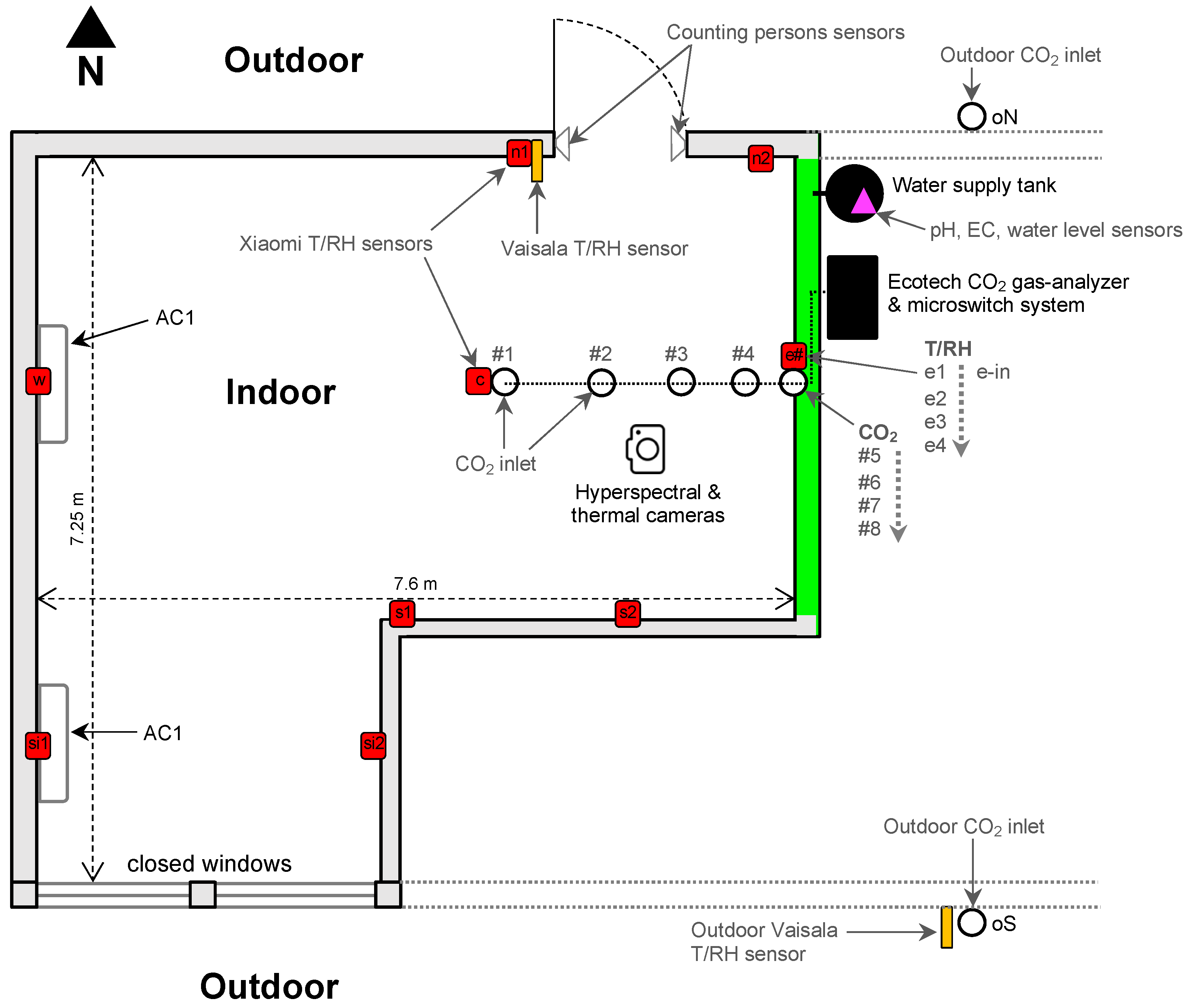
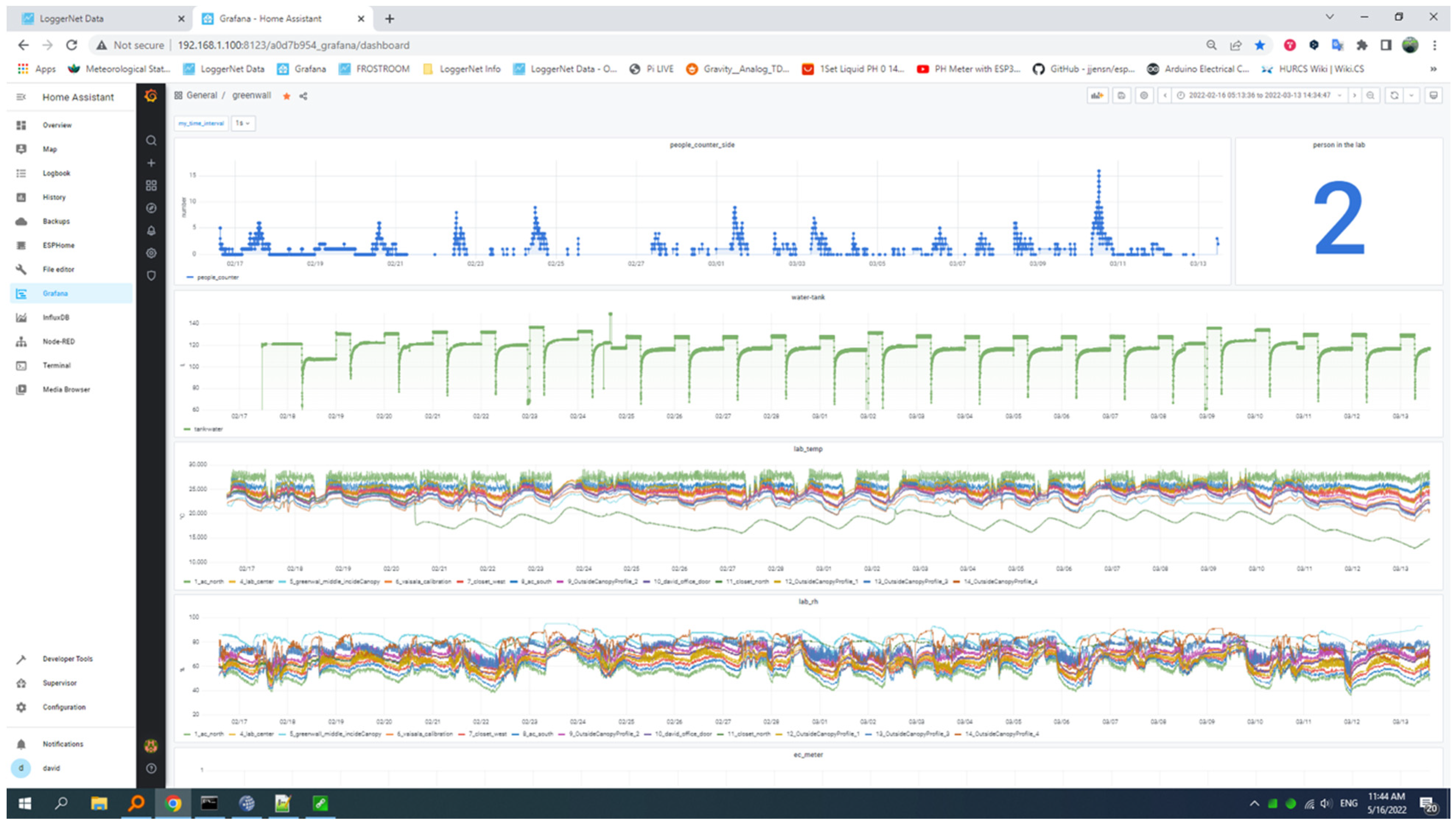
3.2. The Working Space and Its Indoor Environmental Monitoring System

The M&M-VS lab is an Agritech workplace of approximately 46 m2, with a total volume of about 140 m3. The lab is equipped with desktop workstations, and typically 2 to 8 students work in the lab simultaneously. Typical working hours are from 8 am to 8 pm. Air conditioning in the room is set at 25 °C, and fresh air is supplied through a mixing ventilation system (from the top) with an air exchange rate of 0.25–1.5 h−1.
The indoor conditions were continuously monitored via a set of sensors, including air temperature and relative humidity (RH) sensors (T/RH sensors of Xiaomi, Beijing, China, and an HMP155 sensor, Vaisala, Finland) distributed across the room in the horizontal and vertical directions (Figure 2). In addition, a people-counting sensor was placed at the lab entrance to monitor the number of people in the room at any given time. A series of 10 inlet tubes injected air into a gas analyzer (Serinus 31, Ecotech Pty Ltd., Sydney, Australia), located behind the wall, at different distances from the VGW (0.1, 0.35, 0.8, 2, and 3 m from the wall and 0.8 m from the top) and to varying heights near the wall (at a distance of 10 cm from the wall and 0.8, 1.2, 1.9, and 2.5 m from the top) in addition to two external inlet tubes that sample the outdoor air at the northern and southern sides of the building (Figure 2). The eight internal and two outer tubes provided horizontal and vertical CO2 profiles across the transect from the wall towards the room’s center and from the top to the floor, as well as outdoor CO2 conditions.
The CO2 sampling was conducted via a microswitch system that injects air from 10 inlet tubes for 3 min each. The sampled air was streamed from the inlet tube to the gas analyzer at a constant rate using a 1 L reciprocating vacuum pump. To avoid air contamination from the previous tube, we wrote a Python code that excludes the first two minutes of data after the valve opens. That way, we could investigate the “clean” air from the specific opened tube. This resulted in a 30 min cycle of the 10 sampling tubes at different distances and heights from the VGW (see “CO2 inlet” in Figure 2). Air temperature, RH, and solar radiation were also monitored outside the building (Figure 2).
Data were streamed to and displayed in, Grafana, a multiplatform, open-source analytics and interactive data-visualization web application (https://grafana.com; accessed on 1 June 2022). This enables a continuous, real-time data visualization at a relatively high frequency, with some basic, on-the-fly analytical capabilities (Figure 3).

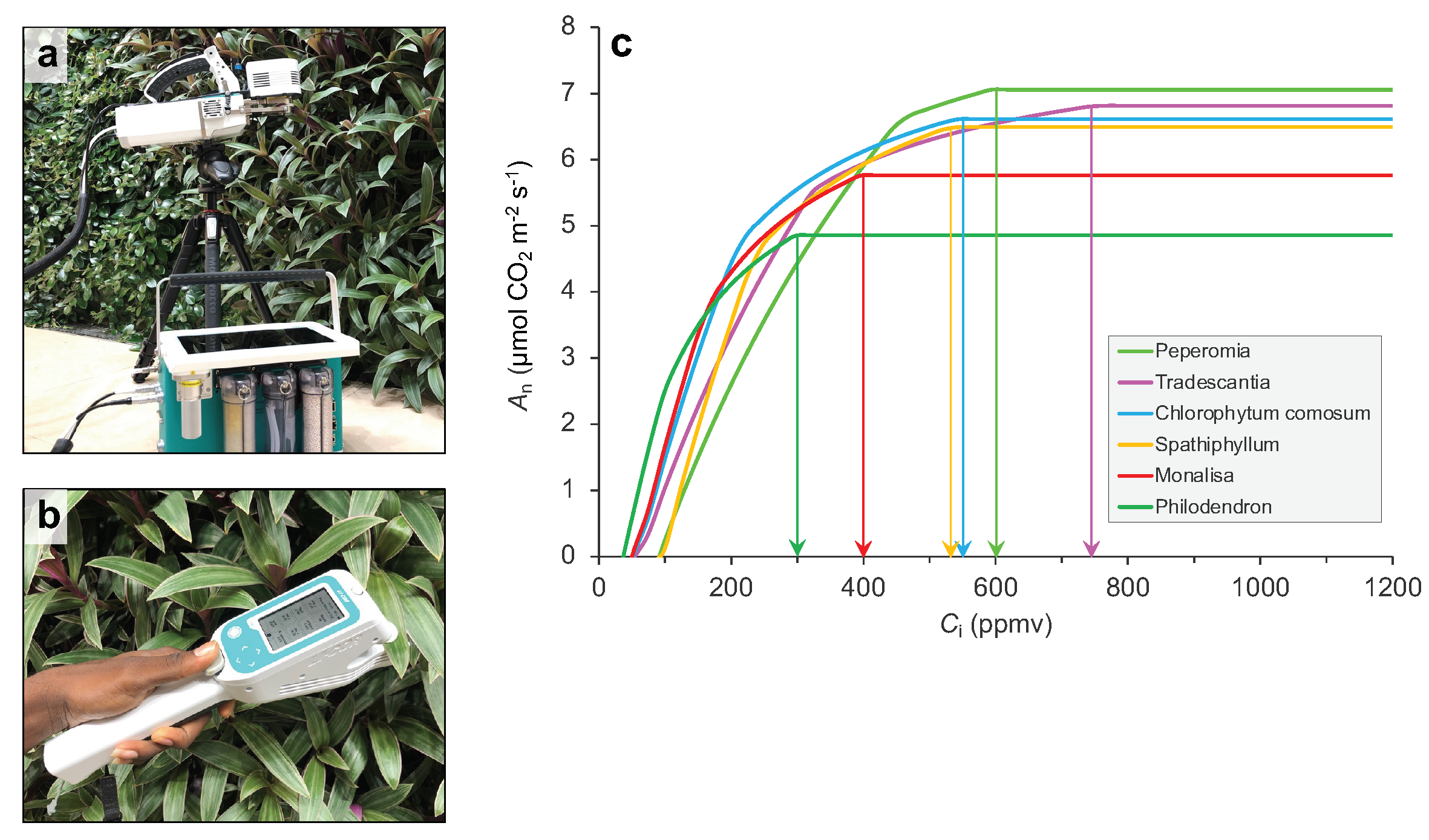
3.3. Leaf Level Gas Exchange Measurements

We used LiCOR devices (LI-6800 and LI-600, LiCOR, NE, USA; Figure 4a,b) to monitor level leaf gas-exchange rates. Measurements of leaf transpiration, CO2 assimilation, and stomatal conductance were conducted periodically once every three weeks on average on each of the six species to characterize their light use efficiencies and carbon uptake capacities. A total of three leaves were sampled per species per date to maintain a minimum interval of time between the leaf measurements and the images. In addition, the actual transpiration was measured with the LI-600 porometer on a total of 60 to 90 random leaves across the wall (10–15 leaves per species) every month.
Our preliminary single leaf results showed that the six species grown on the indoor VGW had a diverse response to increasing ambient CO2 concentrations (Figure 4c).
Since intercellular CO2 concentration (Ci) can be taken as 70% of the ambient concentration in C3 plants [42], the ACi curve can provide information regarding the effectiveness of the species in reducing CO2 levels in the room through the process of carbon assimilation. For example, Peperomia seemed to reach a maximum assimilation rate of ~7 μmol m−2 s−1 at 600 ppmv (light green arrow in Figure 4c). At the same time, Philodendron, which had the lowest response to elevated CO2 with ~5 μmol m−2 s−1, reached its maximum assimilation capacity at a much lower intercellular CO2 concentration (Ci) of only 300 ppmv (dark green arrow in Figure 4c). This means that, under light conditions of 300 μmol photons m−2 s−1, Peperomia was 40% more efficient in reducing indoor CO2 concentrations, with increased assimilation up to 600 ppm. This information can help us design VGWs with specific species at specific light conditions and at the required density and area to provide the most efficient system that reduces indoor CO2 to meet the room’s indoor air quality requirements and customers’ needs.

4. Remote Sensing and Artificial Intelligence for VGWs

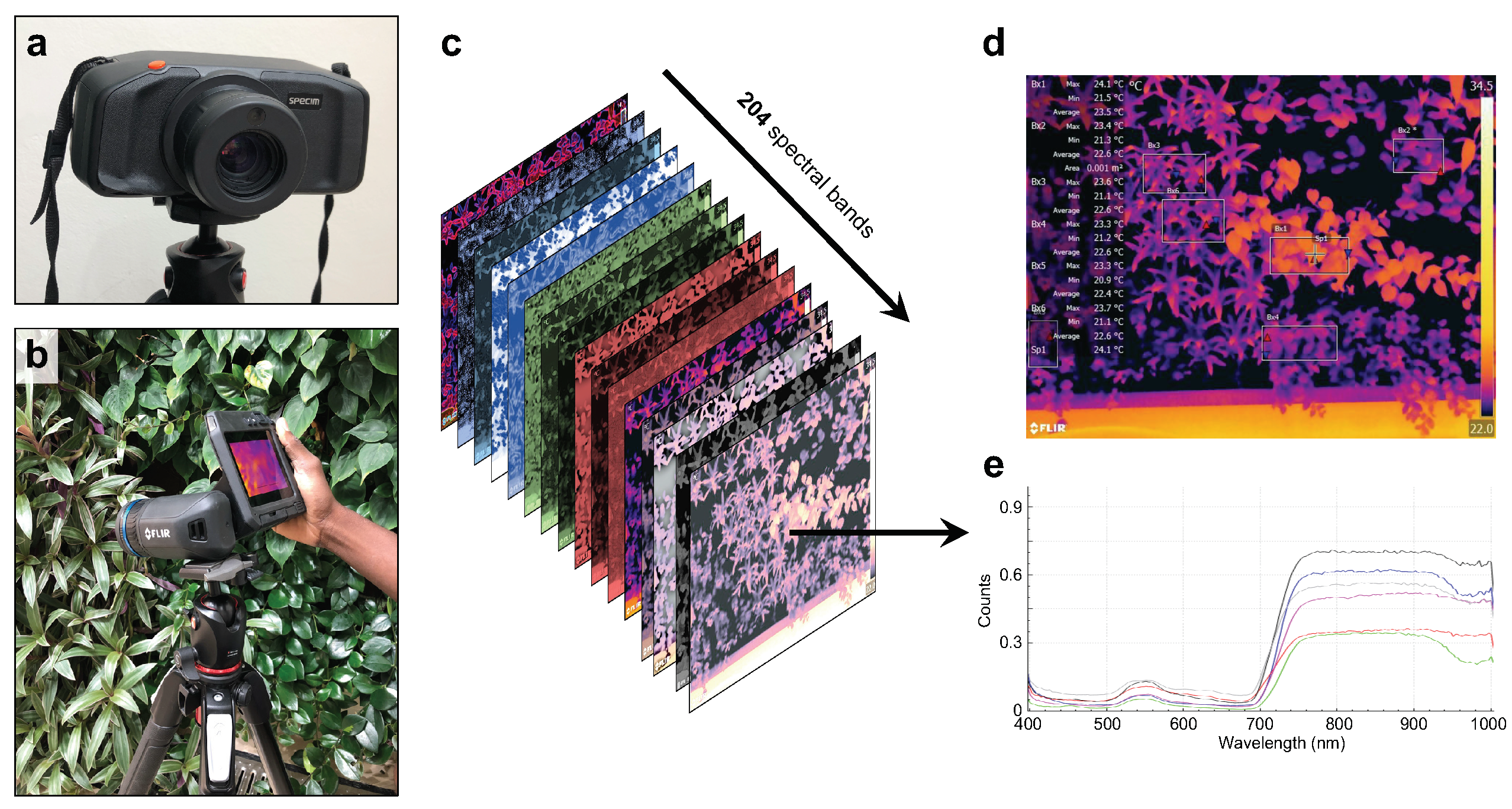
4.1. Creating the Spectral and Thermal Data Collections

The use of remote sensing cameras (sometimes called proximal sensing) can aid in monitoring and managing VGW systems [22]. The idea is to apply techniques borrowed from the precision agriculture field to monitor indoor vertical vegetation. This task often requires using artificial intelligence (AI) to make sense of the high-throughput data generated from such cameras (Figure 5).
In our VGW system, we used hyperspectral and thermal cameras to monitor the wall, while the cameras were placed in the center of the lab in front of the living wall (Figure 2). A SpecimIQ hyperspectral camera (Specim Ltd., Oulu, Finland; Figure 5a) [43] provided spectral information in the 400–1000 nm range, having a total of 204 spectral bands with a 7 nm FWHM bandwidth and a field-of-view (FOV) of 0.55 by 0.55 m at 1 m with a spatial resolution of 512 × 512 pixels. The 204 bands provided a unique spectral signature for each leaf, plant, and species (Figure 5e). This signature could then be used, in combination with gas-exchange data, to develop models that quantify the water use (transpiration) and carbon uptake of the plants (e.g., [26]). These models can be used to monitor the spatial variability across the wall for management purposes.
In addition, a thermal FLIR T560 camera (FLIR Systems, Inc., Wilsonville, OR, USA), with a spatial resolution of 640 × 480 pixels, is used to provide the plant’s leaf surface temperature (Figure 5b,d). Since leaf temperature is usually highly correlated with stomatal conductance and transpiration [29,31], this information can be used to quantify changes in the water use of the plants across the wall. It provides timely information on, for example, stress conditions due to a failure in the irrigation system [44] or plant damage caused by diseases or pests [45].

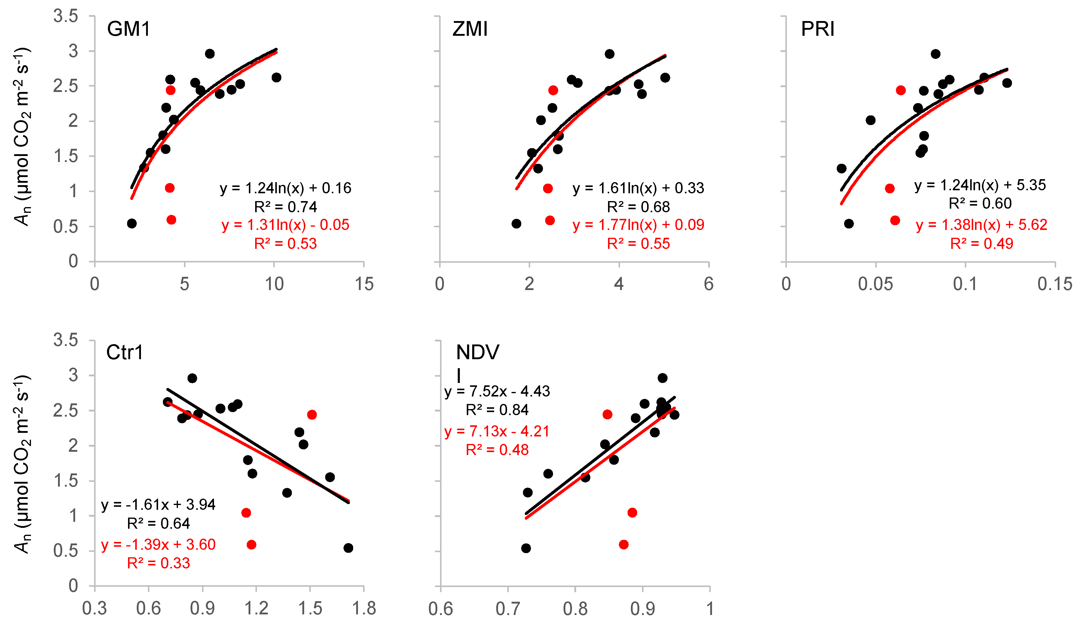
4.2. Remote Sensing of Gas-Exchange Parameters

Several spectral-based vegetation indices were developed to track changes in the vegetation functioning and dynamics using remote sensing tools [46]. These indices can be derived from sensors onboard satellites [47], drones [48], or manually handled cameras [31].
Table 2 presents a few of these indices alongside a brief description of each index and its primary use in previous studies.
Figure 6 shows that these indices had different types of relationships, from linear to curvilinear, with assimilation rate (carbon uptake) measured in leaves of the six species from across the VGW. These relationships could then be used to quantify the amount of carbon dioxide removed from the room’s space and to monitor changes across the wall for management purposes.
Here, we present two examples of the PRI, which is known to be related to photosynthetic activity and, more specifically, to the light use efficiency of the plant through the xanthophyll cycle (i.e., the plant’s ability to use the light for photosynthesis [54,55,56]), and the temperature difference between the leaf surface (derived from the FLIR T560 camera) and the surrounding air (derived from the Xiaomi sensor)—ΔTleaf-air.
Figure 7a shows that the PRI had a positive, linear relationship with carbon assimilation, which is consistent when using all six species. Such a relationship was previously reported for different types of vegetation and different scales [24,25,54,57,58]. In contrast, ΔTleaf-air was negatively correlated to stomatal conductance, meaning that closing of the stomata increased the leaf surface’s temperature through a reduced evaporative cooling, which, in turn, increased ΔTleaf-air (Figure 7b). This negative relationship was previously observed in several tree species and wheat [29,31].

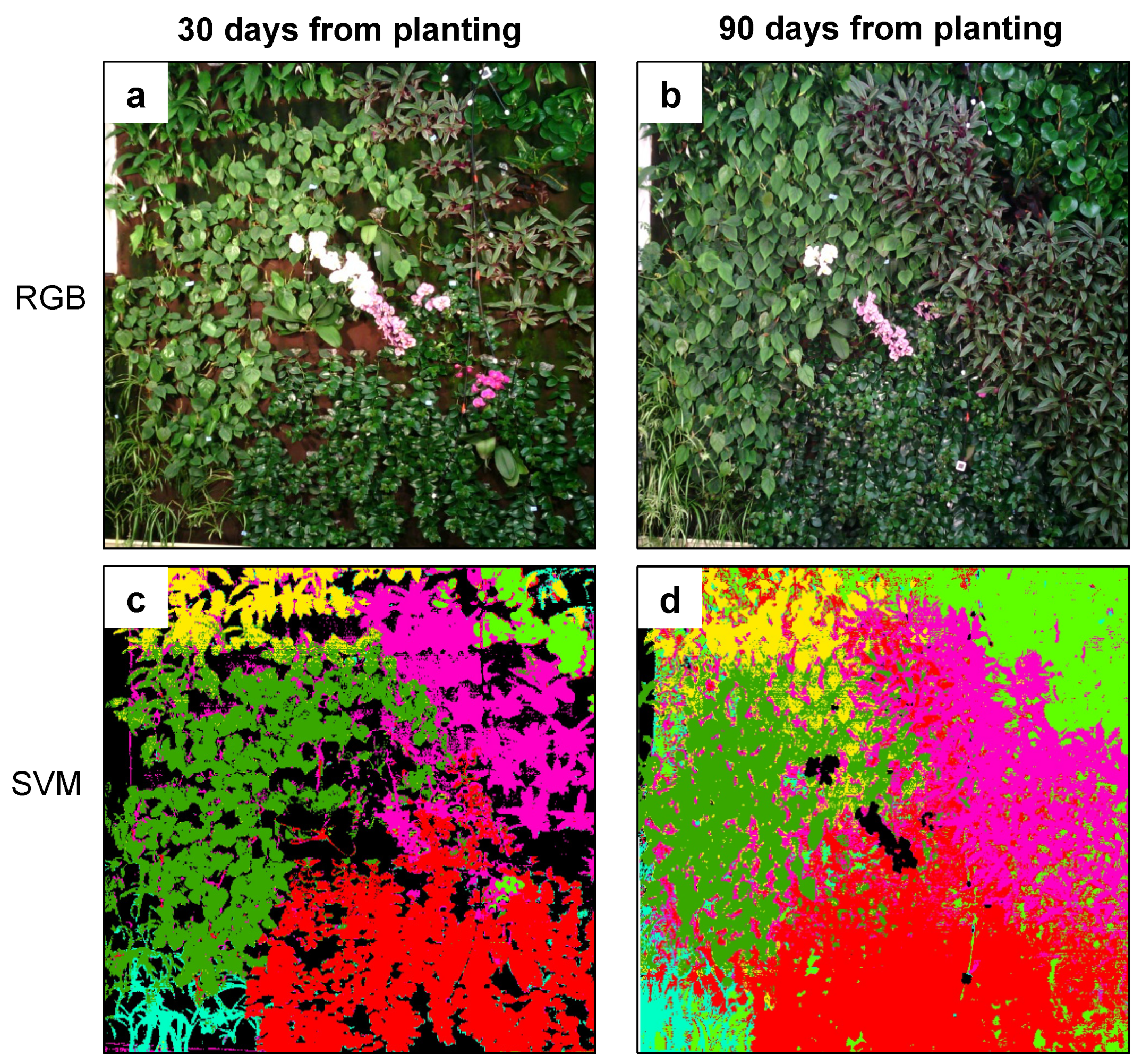
4.3. AI and Machine Learning Supervised Classification for Tracking Vegetation Dynamics

The large number of spectral bands provided by the SpecimIQ camera can be leveraged to automatically distinguish between the species across the VGW, tracking their development through time.
Figure 8 shows results from a supervised classification applied to the 204-spectral band images of the bottom left side of the VGW using a support vector machine (SVM) algorithm [59]. The SVM was trained on the images after passing through a dimensionality reduction to 10 bands using principal component analysis (PCA). The SVM was then run in ArcGIS Pro using the segment attribute data of average chromaticity color, count of pixels, compactness, and rectangularity [60].
Preliminary results of two images, one taken 30 days from planting (Figure 8a,c) and another taken 90 days from planting (Figure 8b,d), showed the evolution and development of the green living wall through time. Species competition was noticed through the expansion of the plant area through the supervised classification images.
Combining spectral- and thermal-based models with the supervised classification maps can enable the tracking of the per-species response to indoor environmental changes. It may also be used to alert when a species is under stressed conditions, enabling better management of the species and the whole VGW, optimizing the efficiency of the living wall in improving indoor conditions.

5. Future Work and Implications for NBS and Urban Farming

Indoor vertical green living wall systems (VGWs) may fulfill NBS targets of air pollution and carbon dioxide reductions and enhance building occupant health, well-being, and comfort conditions [3]. Such indoor and outdoor systems may serve as potential “green” smart city solutions in the future [1,2], especially when such systems are managed with high-tech monitoring tools. Advancements in the Internet of Things (IoT) and cloud technologies are excellent opportunities for leveraging the information acquired through low-cost sensors in monitoring and managing VGWs [61]. However, significant challenges still need to be addressed, such as the spatially continuous monitoring of the living wall, which cannot be easily achieved with simple sensors. This is where precision agriculture tools that include proximal and remote sensing may be combined with IoT and cloud-based systems to provide such crucial information.
In this short paper, we described a first-of-its-kind remote sensing high-throughput indoor VGW system that may serve as a pilot for the automatic (or semi-automatic) monitoring of indoor/outdoor vertical greenery systems. There is still a need for model development to take the unprocessed remote sensing data and produce meaningful information that will aid in managing VGWs (e.g., [26,27,62]). However, combining spectral indices, such as those presented in this study, with gas exchange and other biophysical parameters may help produce a spatially continuous picture of the status of the living wall. Thermal information may also assist in detecting early stresses [22,31] or quantifying the plant’s water use [29]. Such models can produce spatially continuous, real-time status maps of the VGW.
The next step is to use this information to learn about the functioning of VGWs and their feedback and impact on the surrounding environment. Such a step is essential to improve indoor and outdoor conditions more efficiently. Artificial intelligence (AI) may play a critical role in this task. AI algorithms are already being used to accurately acquire information about indoor environmental quality from low-cost sensors [63]. In this context, AI can be combined with remote sensing to detect plant disease, which may assist in managing VGWs [64]. Hyperspectral data can be leveraged to alert on disease development across the living wall even before it is detected by our bare eyes or the use of RGB images.
Anomaly detection using AI was also shown to support the predictive maintenance of VGWs’ indoor environment [65]. The core task to achieve VGWs’ predictive maintenance is to recognize anomalous changes as early as possible across the wall (from time series of remote sensing images) and in the indoor environment (from low-cost sensors spread across the room). A decision support system can then be used to control and manipulate the VGW conditions through, for example, changing the light conditions, irrigation scheme, and room ventilation rate. This idea of combining low-cost sensors, remote sensing imaging, and AI in a decision support system is already being implemented in conventional agriculture (e.g., [66,67,68]). However, this might require special adjustments to indoor VGW systems, which must be guided through further research. In the meantime, more VGW monitoring systems such as the one described in this paper may open new opportunities to develop smart techniques for managing VGWs and study these systems under different conditions and with various plant species and monitoring solutions.

Author Contributions

Conceptualization, D.H.; Data curation, Y.Y., G.M. and Y.M.; Formal analysis, D.H., Y.Y., G.M. and Y.M.; Investigation, D.H., Y.Y. and G.M.; Methodology, D.H., Y.Y., G.M. and Y.M.; Project administration, D.H.; Software, Y.M.; Supervision, D.H.; Writing—original draft, D.H.; Writing—review & editing, D.H. and Y.Y. All authors have read and agreed to the published version of the manuscript.

Funding

This research received no external funding.

Data Availability Statement

The data presented in this study are available on request from the corresponding author.

Acknowledgments

Y.Y. thanks Israel’s Women League for partly supporting his M.Sc. studies and research in the Advanced School for Environmental Studies. The authors thank Richard Rozenbaum from Richard vertical gardens (www.rrgardening.co.il/en/vertical-gardens; accessed on 1 July 2022) for constructing the VGW in our lab, EnviroManager©, Gil Lerner for building and installing the gas analyzer microswitch system, and Jiang Duo for helping with preparing the ACi curve. The camera icon in Figure 2 was created by Good Ware (www.flaticon.com; accessed on 1 January 2022).

Conflicts of Interest

The authors declare no conflict of interest.

References

  1. Kabisch, N.; Frantzeskaki, N.; Pauleit, S.; Naumann, S.; Davis, M.; Artmann, M.; Haase, D.; Knapp, S.; Korn, H.; Stadler, J.; et al. Nature-based solutions to climate change mitigation and adaptation in urban areas. Ecol. Soc. 2016, 21, 15. [Google Scholar] [CrossRef] [Green Version]
  2. Seto, K.C.; Golden, J.S.; Alberti, M.; Turner, B.L. Sustainability in an urbanizing planet. Proc. Natl. Acad. Sci. USA 2017, 114, 8935–8938. [Google Scholar] [CrossRef] [Green Version]
  3. Sanchez Rodriguez, R.; Ürge-Vorsatz, D.; Barau, A.S. Sustainable Development Goals and climate change adaptation in cities. Nat. Clim. Chang. 2018, 8, 181–183. [Google Scholar] [CrossRef]
  4. European Commission. Towards an EU Research and Innovation Policy Agenda for Nature-Based Solutions and Re-Naturing Cities. Final Report of the Horizon 2020 Expert Group on “NatureBased Solutions and Re-Naturing Cities”; Publications Office of the European Union: Brussels, Belgium, 2015. [Google Scholar]
  5. Nan, X.; Yan, H.; Wu, R.; Shi, Y.; Bao, Z. Assessing the thermal performance of living wall systems in wet and cold climates during the winter. Energy Build. 2020, 208, 109680. [Google Scholar] [CrossRef]
  6. De Jesus, M.P.; Lourenço, J.M.; Arce, R.M.; Macias, M. Green façades and in situ measurements of outdoor building thermal behaviour. Build. Environ. 2017, 119, 11–19. [Google Scholar] [CrossRef] [Green Version]
  7. Gunawardena, K.; Steemers, K. Living walls in indoor environments. Build. Environ. 2019, 148, 478–487. [Google Scholar] [CrossRef]
  8. Rotem-Mindali, O.; Michael, Y.; Helman, D.; Lensky, I.M. The role of local land-use on the urban heat island effect of Tel Aviv as assessed from satellite remote sensing. Appl. Geogr. 2015, 56, 145–153. [Google Scholar] [CrossRef]
  9. Pérez-Urrestarazu, L.; Fernández-Cañero, R.; Franco, A.; Egea, G. Influence of an active living wall on indoor temperature and humidity conditions. Ecol. Eng. 2016, 90, 120–124. [Google Scholar] [CrossRef]
  10. Abdo, P.; Huynh, B.P. Effect of Passive Green Wall Modules on Air Temperature and Humidity; American Society of Mechanical Engineers: New York, NY, USA, 2018. [Google Scholar]
  11. Irga, P.J.; Paull, N.J.; Abdo, P.; Torpy, F.R. An assessment of the atmospheric particle removal efficiency of an in-room botanical biofilter system. Build. Environ. 2017, 115, 281–290. [Google Scholar] [CrossRef]
  12. Torpy, F.; Zavattaro, M. Bench-study of green-wall plants for indoor air pollution reduction. J. Living Archit. 2018, 5, 1–15. [Google Scholar] [CrossRef]
  13. Pettit, T.; Irga, P.J.; Torpy, F.R. The in situ pilot-scale phytoremediation of airborne VOCs and particulate matter with an active green wall. Air Qual. Atmos. Health 2019, 12, 33–44. [Google Scholar] [CrossRef]
  14. Torpy, F.; Zavattaro, M.; Irga, P. Green wall technology for the phytoremediation of indoor air: A system for the reduction of high CO2 concentrations. Air Qual. Atmos. Health 2017, 10, 575–585. [Google Scholar] [CrossRef]
  15. Torpy, F.; Clements, N.; Pollinger, M.; Dengel, A.; Mulvihill, I.; He, C.; Irga, P. Testing the single-pass VOC removal efficiency of an active green wall using methyl ethyl ketone (MEK). Air Qual. Atmos. Health 2018, 11, 163–170. [Google Scholar] [CrossRef] [Green Version]
  16. Gawrońska, H.; Bakera, B. Phytoremediation of particulate matter from indoor air by Chlorophytum comosum L. plants. Air Qual. Atmos. Health 2015, 8, 265–272. [Google Scholar] [CrossRef] [Green Version]
  17. Charoenkit, S.; Yiemwattana, S. Living walls and their contribution to improved thermal comfort and carbon emission reduction: A review. Build. Environ. 2016, 105, 82–94. [Google Scholar] [CrossRef]
  18. Soreanu, G. 12—Biotechnologies for Improving Indoor Air Quality; Pacheco-Torgal, F., Rasmussen, E., Granqvist, C.-G., Ivanov, V., Kaklauskas, A., Makonin, S.B.T.-S.-U.C., Eds.; Woodhead Publishing: Thorston, UK, 2016; pp. 301–328. ISBN 978-0-08-100546-0. [Google Scholar]
  19. Irga, P.J.; Pettit, T.J.; Torpy, F.R. The phytoremediation of indoor air pollution: A review on the technology development from the potted plant through to functional green wall biofilters. Rev. Environ. Sci. Biotechnol. 2018, 17, 395–415. [Google Scholar] [CrossRef]
  20. Wang, Z.; Zhang, J.S. Characterization and performance evaluation of a full-scale activated carbon-based dynamic botanical air filtration system for improving indoor air quality. Build. Environ. 2011, 46, 758–768. [Google Scholar] [CrossRef]
  21. Allen, J.G.; MacNaughton, P.; Satish, U.; Santanam, S.; Vallarino, J.; Spengler, J.D. Associations of cognitive function scores with carbon dioxide, ventilation, and volatile organic compound exposures in office workers: A controlled exposure study of green and conventional office environments. Environ. Health Perspect. 2016, 124, 805–812. [Google Scholar] [CrossRef] [Green Version]
  22. Yuan, X.; Laakso, K.; Davis, C.D.; Guzmán Q., J.A.; Meng, Q.; Sanchez-Azofeifa, A. Monitoring the Water Stress of an Indoor Living Wall System Using the “Triangle Method”. Sensors 2020, 20, 3261. [Google Scholar] [CrossRef]
  23. Peñuelas, J.; Marino, G.; LLusia, J.; Morfopoulos, C.; Farré-Armengol, G.; Filella, I. Photochemical reflectance index as an indirect estimator of foliar isoprenoid emissions at the ecosystem level. Nat. Commun. 2013, 4, 2604. [Google Scholar] [CrossRef] [Green Version]
  24. Peñuelas, J.; Garbulsky, M.F.; Filella, I. Photochemical reflectance index (PRI) and remote sensing of plant CO2 uptake. New Phytol. 2011, 191, 596–599. [Google Scholar] [CrossRef] [PubMed]
  25. Zhang, C.; Filella, I.; Garbulsky, F.M.; Peñuelas, J. Affecting Factors and Recent Improvements of the Photochemical Reflectance Index (PRI) for Remotely Sensing Foliar, Canopy and Ecosystemic Radiation-Use Efficiencies. Remote Sens. 2016, 8, 677. [Google Scholar] [CrossRef] [Green Version]
  26. Helman, D.; Lensky, I.M.; Osem, Y.; Rohatyn, S.; Rotenberg, E.; Yakir, D. A biophysical approach using water deficit factor for daily estimations of evapotranspiration and CO2 uptake in Mediterranean environments. Biogeosciences 2017, 14, 3909–3926. [Google Scholar] [CrossRef] [Green Version]
  27. Helman, D.; Bonfil, D.J.; Lensky, I.M. Crop RS-Met: A biophysical evapotranspiration and root-zone soil water content model for crops based on proximal sensing and meteorological data. Agric. Water Manag. 2019, 211, 210–219. [Google Scholar] [CrossRef]
  28. Helman, D.; Lensky, I.M.; Bonfil, D.J. Early prediction of wheat grain yield production from root-zone soil water content at heading using Crop RS-Met. Field Crops Res. 2019, 232, 11–23. [Google Scholar] [CrossRef]
  29. Lapidot, O.; Ignat, T.; Rud, R.; Rog, I.; Alchanatis, V.; Klein, T. Use of thermal imaging to detect evaporative cooling in coniferous and broadleaved tree species of the Mediterranean maquis. Agric. For. Meteorol. 2019, 271, 285–294. [Google Scholar] [CrossRef]
  30. Cohen, Y.; Alchanatis, V.; Saranga, Y.; Rosenberg, O.; Sela, E.; Bosak, A. Mapping water status based on aerial thermal imagery: Comparison of methodologies for upscaling from a single leaf to commercial fields. Precis. Agric. 2017, 18, 801–822. [Google Scholar] [CrossRef]
  31. Mulero, G.; Jiang, D.; Bonfil, D.J.; Helman, D. Use of thermal imaging and the Photochemical Reflectance Index (PRI) to detect wheat response to elevated CO2 and drought. Under Rev. 2022. [Google Scholar]
  32. Blanc, P. The Vertical Garden: From Nature to the City, 2nd ed.; W.W. Norton: New York, NY, USA, 2012. [Google Scholar]
  33. Johnstone, G. How to Grow Peperomia Obtusifolia (Baby Rubber Plants). Available online: https://www.thespruce.com/peperomia-obtusifolia-growing-guide-5271088 (accessed on 1 June 2022).
  34. ASPCA Blunt Leaf Peperomia. Available online: https://www.aspca.org/pet-care/animal-poison-control/toxic-and-non-toxic-plants/blunt-leaf-peperomia (accessed on 1 June 2022).
  35. Richard, A.; Ramey, V. Invasive and Nonnative Plants You Should Know–Recognition Cards; University of Florida-IFAS Publication # SP: Gainesville, FL, USA, 2007. [Google Scholar]
  36. Langeland, K.A.; Burks, K.C. Identification & Biology of Non-Native Plants in Florida’s Natural Areas 1998; University of Florida: Gainesville, FL, USA, 2013; pp. 138–157. [Google Scholar]
  37. Extension Gardener Tradescantia Spathacea. Available online: https://plants.ces.ncsu.edu/plants/tradescantia-spathacea/ (accessed on 1 June 2022).
  38. Rzhepakovsky, I.V.; Areshidze, D.A.; Avanesyan, S.S.; Grimm, W.D.; Filatova, N.V.; Kalinin, A.V.; Kochergin, S.G.; Kozlova, M.A.; Kurchenko, V.P.; Sizonenko, M.N.; et al. Phytochemical Characterization, Antioxidant Activity, and Cytotoxicity of Methanolic Leaf Extract of Chlorophytum Comosum (Green Type) (Thunb.) Jacq. Molecules 2022, 27, 762. [Google Scholar] [CrossRef]
  39. Wolverton, B. Plants and soil microorganisms: Removal of formaldehyde, xylene, and ammonia from the indoor environment. J. Miss. Acad. Sci. 1993, 38, 11. [Google Scholar]
  40. Turner, C. Ten Poisonous Indoor Plants Your Children and Pets Should Avoid. Available online: https://blog.mytastefulspace.com/2020/03/04/poisonous-indoor-plants/ (accessed on 1 June 2022).
  41. USDA Taxon: Philodendron Hederaceum (Jacq.) Schott. Available online: https://npgsweb.ars-grin.gov/gringlobal/taxon/taxonomydetail?id=102625 (accessed on 1 June 2022).
  42. Wong, S.C.; Cowan, I.R.; Farquhar, G.D. Stomatal conductance correlates with photosynthetic capacity. Nature 1979, 282, 424–426. [Google Scholar] [CrossRef]
  43. Behmann, J.; Acebron, K.; Emin, D.; Bennertz, S.; Matsubara, S.; Thomas, S.; Bohnenkamp, D.; Kuska, M.T.; Jussila, J.; Salo, H.; et al. Specim IQ: Evaluation of a New, Miniaturized Handheld Hyperspectral Camera and Its Application for Plant Phenotyping and Disease Detection. Sensors 2018, 18, 441. [Google Scholar] [CrossRef] [Green Version]
  44. Ben-Gal, A.; Agam, N.; Alchanatis, V.; Cohen, Y.; Yermiyahu, U.; Zipori, I.; Presnov, E.; Sprintsin, M.; Dag, A. Evaluating water stress in irrigated olives: Correlation of soil water status, tree water status, and thermal imagery. Irrig. Sci. 2009, 27, 367–376. [Google Scholar] [CrossRef]
  45. Zhang, J.; Huang, Y.; Pu, R.; Gonzalez-Moreno, P.; Yuan, L.; Wu, K.; Huang, W. Monitoring plant diseases and pests through remote sensing technology: A review. Comput. Electron. Agric. 2019, 165, 104943. [Google Scholar] [CrossRef]
  46. Helman, D. Land surface phenology: What do we really ‘see’ from space? Sci. Total Environ. 2018, 618, 665–673. [Google Scholar] [CrossRef]
  47. Helman, D.; Mussery, A. Using Landsat satellites to assess the impact of check dams built across erosive gullies on vegetation rehabilitation. Sci. Total Environ. 2020, 730, 138873. [Google Scholar] [CrossRef]
  48. Manfreda, S.; McCabe, M.F.; Miller, P.E.; Lucas, R.; Madrigal, V.P.; Mallinis, G.; Ben Dor, E.; Helman, D.; Estes, L.; Ciraolo, G.; et al. On the use of unmanned aerial systems for environmental monitoring. Remote Sens. 2018, 10, 641. [Google Scholar] [CrossRef] [Green Version]
  49. Gitelson, A.A.; Merzlyak, M.N. Remote estimation of chlorophyll content in higher plant leaves. Int. J. Remote Sens. 1997, 18, 2691–2697. [Google Scholar] [CrossRef]
  50. Zarco-Tejada, P.J.; Miller, J.R.; Noland, T.L.; Mohammed, G.H.; Sampson, P.H. Scaling-up and model inversion methods with narrowband optical indices for chlorophyll content estimation in closed forest canopies with hyperspectral data. IEEE Trans. Geosci. Remote Sens. 2001, 39, 1491–1507. [Google Scholar] [CrossRef] [Green Version]
  51. Gamon, J.A.; Penuelas, J.; Field, C.B. A Narrow-Waveband Spectral Index That Tracks Diurnal Changes in Photosynthetic Efficiency. Remote Sens. Environ. 1992, 41, 35–44. [Google Scholar] [CrossRef]
  52. Carter, G.A. Ratios of leaf reflectances in narrow wavebands as indicators of plant stress. Int. J. Remote Sens. 1994, 15, 517–520. [Google Scholar] [CrossRef]
  53. Rouse, J.W.; Haas, R.H.; Schell, J.A.; Deering, D.W.; Harlan, J.C. Monitoring the Vernal Advancement and Retrogradation of Natural Vegetation, O F Natural; Texas A&M Univ.: College Station, TX, USA, 1974. [Google Scholar]
  54. Garbulsky, M.F.; Peñuelas, J.; Gamon, J.; Inoue, Y.; Filella, I. The photochemical reflectance index (PRI) and the remote sensing of leaf, canopy and ecosystem radiation use efficiencies: A review and meta-analysis. Remote Sens. Environ. 2011, 115, 281–297. [Google Scholar] [CrossRef]
  55. Filella, I.; Peñuelas, J.; Llorens, L.; Estiarte, M. Reflectance assessment of seasonal and annual changes in biomass and CO2 uptake of a Mediterranean shrubland submitted to experimental warming and drought. Remote Sens. Environ. 2004, 90, 308–318. [Google Scholar] [CrossRef]
  56. Gamon, J.A.; Serrano, L.; Surfus, J.S. The photochemical reflectance index: An optical indicator of photosynthetic radiation use efficiency across species, functional types, and nutrient levels. Oecologia 1997, 112, 492–501. [Google Scholar] [CrossRef]
  57. Amthor, J.S. Scaling CO2-photosynthesis relationships from the leaf to the canopy. Photosynth. Res. 1994, 39, 321–350. [Google Scholar] [CrossRef]
  58. Magney, T.S.; Vierling, L.A.; Eitel, J.U.H.; Huggins, D.R.; Garrity, S.R. Response of high frequency Photochemical Reflectance Index (PRI) measurements to environmental conditions in wheat. Remote Sens. Environ. 2016, 173, 84–97. [Google Scholar] [CrossRef]
  59. Cortes, C.; Vapnik, V. Support-vector networks. Mach. Learn. 1995, 20, 273–297. [Google Scholar] [CrossRef]
  60. ESRI ArcGIS PRO, Version 2.9. Redlands, California. 2019. Available online: https://www.esri.com/en-us/about/about-esri/company (accessed on 1 July 2022).
  61. Liu, Y.; Hassan, K.A.; Karlsson, M.; Weister, O.; Gong, S. Active Plant Wall for Green Indoor Climate Based on Cloud and Internet of Things. IEEE Access 2018, 6, 33631–33644. [Google Scholar] [CrossRef]
  62. Helman, D.; Bahat, I.; Netzer, Y.; Ben-Gal, A.; Alchanatis, V.; Peeters, A.; Cohen, Y. Using time series of high-resolution planet satellite images to monitor grapevine stem water potential in commercial vineyards. Remote Sens. 2018, 10, 1615. [Google Scholar] [CrossRef] [Green Version]
  63. Troncoso-Pastoriza, F.; Martínez-Comesaña, M.; Ogando-Martínez, A.; López-Gómez, J.; Eguía-Oller, P.; Febrero-Garrido, L. IoT-based platform for automated IEQ spatio-temporal analysis in buildings using machine learning techniques. Autom. Constr. 2022, 139, 104261. [Google Scholar] [CrossRef]
  64. Saleem, M.H.; Potgieter, J.; Arif, K.M. Plant Disease Detection and Classification by Deep Learning. Plants 2019, 8, 468. [Google Scholar] [CrossRef] [PubMed] [Green Version]
  65. Liu, Y.; Pang, Z.; Karlsson, M.; Gong, S. Anomaly detection based on machine learning in IoT-based vertical plant wall for indoor climate control. Build. Environ. 2020, 183, 107212. [Google Scholar] [CrossRef]
  66. Kpienbaareh, D.; Kansanga, M.; Luginaah, I. Examining the potential of open source remote sensing for building effective decision support systems for precision agriculture in resource-poor settings. GeoJournal 2019, 84, 1481–1497. [Google Scholar] [CrossRef]
  67. Ennouri, K.; Smaoui, S.; Gharbi, Y.; Cheffi, M.; Ben Braiek, O.; Ennouri, M.; Triki, M.A. Usage of Artificial Intelligence and Remote Sensing as Efficient Devices to Increase Agricultural System Yields. J. Food Qual. 2021, 2021, 6242288. [Google Scholar] [CrossRef]
  68. Jie, Q. Precision and intelligent agricultural decision support system based on big data analysis. Acta Agric. Scand. Sect. B—Soil Plant Sci. 2022, 72, 401–414. [Google Scholar] [CrossRef]
Figure 1. Front view of (a) the VGW with its six main species and (b) the light intensity conditions across the wall (μmol photons m−2 s−1). Light intensity was measured perpendicular to the wall in 120 points (leaves) across the wall, with an average distance of 30 cm from each other. The vertical map shown in (b) was generated using multilevel b-spline interpolation in QGIS.
Remotesensing 14 03485 g001
Figure 2. Plan view of the M&M-VS lab with its VGW monitoring system. Two air-conditioning (AC) systems operate in the room at a fixed temperature of 25 °C in addition to a ventilation system (from the top). Green indicates the location of the living wall. In red are the low-cost temperature/RH sensors. Hollowed circles indicate inlet tubes that sample the air in the room and outside the building (oS and oN), with the air flowing from the tube to a microswitch system and a gas analyzer behind the wall (black rectangle). Water is supplied through an automatic drip system pumped from a tank behind the wall (black circle). Sensors of pH, EC, and water level are connected to the tank (pink triangle). Notice that there are additional T/RH sensors and inlet tubes near the wall (approx. 10 cm from the wall) at different heights from the top for vertical measurements. Another T/RH sensor (e-in) was placed inside the canopy. Data stream in real time to an interactive visualization web application (Grafana) installed on a computer in the lab.
Remotesensing 14 03485 g002
Figure 3. Screenshot of the Grafana interactive visualization web application (https://grafana.com; accessed on 1 June 2022), showing from top to bottom real-time data of the number of persons (blue), the water level at the tank (green), temperature, and RH conditions from the sensors inside the workplace.
Remotesensing 14 03485 g003
Figure 4. The LiCOR (a) LI–6800 gas-exchange system and (b) LI–600 Porometer. (c) Response to intercellular CO2 concentrations (Ci, measured in μmol CO2 m−2 s−1) of the six species grown on the vertical wall in the lab. Vertical arrows in (c) indicate the intercellular CO2 level at which the plants reach the maximum assimilation rate (Amax-C). The Ci is usually ~70% of the ambient CO2 concentrations. Measurements were conducted under cell conditions of RH of 55%, temperature of 25 °C, and CO2 flow rate of 300 μmol s−1. Images were taken by D. Helman.
Remotesensing 14 03485 g004
Figure 5. (a) the SpecimIQ hyperspectral camera and (b) the FLIR T560 thermal camera used to monitor the indoor VGW. (c) Illustration of multiband acquisition of the spectral images from the SpecimIQ data (204 bands in the range of 400–1000 nanometer) and (d) a thermal image of the wall acquired from the FLIR T560 camera. (e) Spectral signal of specific pixels from the VGW image. Images (a,b) were taken by D. Helman.
Remotesensing 14 03485 g005
Figure 6. Association between CO2 assimilation rate (An; μmol CO2 m−2 s−1), measured by the LI–6800 system, and several spectral indices (see Table 2) calculated from the hyperspectral images, showing linear (for NDVI and Ctr1) and curvilinear (for GM1, ZMI, and PRI) relationships. Dots represent leaf measurements on a specific date (10 May 2021) taken from the six species grown across the wall. Red dots are the leaf measurements of the Philodendron plants, which displayed relatively low An (see also Figure 4), sometimes even within the detection level of the measurement system. All models, excluding the Philodendron, were statistically significant at p < 0.05.
Remotesensing 14 03485 g006
Figure 7. Linear relationships between (a) CO2 assimilation rate (An; μmol CO2 m−2 s−1) and the photochemical reflectance index (PRI; Table 2) and (b) stomatal conductance (gs; mol m−2 s−1) and the temperature difference between the leaf (from the FLIR T560 camera) and the air (ΔTleaf-air; °C). Each point on the graphs is the average of several leaves of a single species, while bars represent the standard deviation.
Remotesensing 14 03485 g007
Figure 8. (a,b) RGB images of the bottom left side of the wall and (c,d) an automatic supervised classification of the species derived from the hyperspectral data by use of the support vector machine (SVM) algorithm; (a,c) correspond to an image taken 30 days after planting and (b,d) to an image taken 90 days after planting. Images show the development of the wall through species competition for space, while SVM enabled detecting such changes automatically.
Remotesensing 14 03485 g008
Table 1. The six species planted in the VGW.
Scientific NameCommon NameC-PathwayNative AreaOptimal Growth Temperatures (°C)
Peperomia obtusifoliaBaby rubber plantC3Mexico, South America, and West Indies16–26
Tradescantia spathaceaMoses in the cradle or wondering jewC3Southern Mexico, Belize, Guatemala14–27
Chlorophytum comosumSpider plantC3South Africa15–30
Spathiphyllum wallisii RegelPeace lilyC3Central America15–30
Aeschynanthus radicans “Monalisa”Monalisa or lipstick plantC3Malaysia15–30
Philodendron hederaceumPhilodendron C3North and South America15–26
Table 2. An overview of six spectral vegetation indices that were used in this study.
IndexFull NameFormulaMain Characteristics and Uses
GM1 [49]Gitelson and Merzlyak index 1 750   nm 550   nm The GM1 was developed based on the sensitivity of the 550 nm band to a wide range of chlorophyll variations. It is a useful index for monitoring plant chlorophyll content and photosynthetic capacity.
ZMI [50]Zarco-Tejada and Miller index 750   nm 710   nm The ZMI, based on the red-edge band, was developed to assess changes in available pigment content in leaves and over canopies.
PRI [51]Photochemical reflectance index 531   nm     570   nm 531   nm   +   570   nm The PRI uses the 531 nm band, which is sensitive to variations in the dissipation of light energy via xanthophyll de-epoxidation. It is related to the fast transition in the xanthophyll cycle, making it a good proxy of the plant light use efficiency, an important factor in the photosynthetic process.
Ctr1 [52]Carter index 1 695   nm 420   nm The Ctr1 features the 695 and 420 nm bands, which are sensitive to changes in total chlorophyll concentrations, especially under stress. It has been used for the early detection of stresses in plants.
NDVI [53]Normalized difference vegetation index 790   nm     670   nm 790   nm   +   670   nm The NDVI is the most commonly used vegetation index in proximal and remote sensing [46]. It has been used to measure the state of plant health as well as its phenology and leaf area index. It is also a useful index for estimating vegetation biomass and productivity [47].
Publisher’s Note: MDPI stays neutral with regard to jurisdictional claims in published maps and institutional affiliations.

