
A Newly Developed Tool for the Post-Processing of GPR Time-Slices in A GIS Environment


1
Department for Innovation in Biological, Agro-Food and Forest Systems (DIBAF), Università Degli Studi Della Tuscia, 01100 Viterbo, Italy
2
Department of Linguistic, Literary, Historical, Philosophical and Legal Studies (DISTU), Università Degli Studi Della Tuscia, 01100 Viterbo, Italy
*
Author to whom correspondence should be addressed.
Remote Sens. 2022, 14(14), 3459; https://doi.org/10.3390/rs14143459
Submission received: 15 May 2022
/
Revised: 12 July 2022
/
Accepted: 13 July 2022
/
Published: 19 July 2022
/
Corrected: 16 December 2022
(This article belongs to the Special Issue Advances in Ground-Penetrating Radar for Archaeology)
Abstract
:Ground-penetrating radar (GPR) is a precious and reliable research tool broadly used in archaeology because of its capacity to produce three-dimensional data about features preserved underground, such as buildings, infrastructures, and burials, as well as building rubble. GPR data (time-slices) management and exploitation in Geographic Information Systems (GIS) is mostly limited to the visualization and the manual interpretation and mapping of separate single time-slices. This study presents a newly developed plug-in designed to automatically post-process GPR time-slices in a GIS environment, to identify anomalies, and to produce a synchronic view of them. This map product, when combined with a DTM, results in a 2D map of subsurface anomalies which shows the absolute height of features above sea level, thus offering a comprehensive view of the three-dimensional configuration of the subsurface features identified. The paper illustrates the pixel-based processing chain of the plug-in and the results of the tests carried out in the case study of the Roman town of Falerii Novi (Italy), on the basis of high-resolution open access GPR data recently collected by the University of Cambridge and Ghent.
1. Introduction
Ground Penetrating Radar (GPR) is a geophysical tool used for the survey of underground features in archaeology [1,2,3,4,5], the prospection and the state of conservation assessment in historical buildings [6,7,8], as well as in other research and professional fields, such as geology and civil engineering [9,10,11,12]. It can detect underground structures, canalizations, burials, and tentatively stratigraphic discontinuities in soil [13]. GPR data processing is currently conducted by using specific informatics tools, which allow for the elaboration, cleaning, and enhancing of raw data to produce vertical profiles and horizontal time-slices–i.e., raster images of the subsoil as layers located at different depths, where depth is calculated on the base of the wave travel time and wave velocity (depth = two-way travel time × wave velocity/2).
Some of these software tools are also used to achieve a 3D visualization of GPR time-slices, such as GPR-Slice where time-slices and vertical profiles can be visualized within a cube, meaning in two dimensions but with a three-dimensional impression. Furthermore, various studies address the issue of managing large datasets and their interpretation by exploring possible procedures to identify and model archaeological features from GPR data [14,15,16,17,18]. Other significant experiences integrated GPR and resistivity data, both having a three-dimensional nature, to obtain a 3D visualization [19,20,21]. Nevertheless, these operations are mainly done by tools that, on the one side, cannot be integrated into a GIS environment, and, on the other, are often proprietary software.
On the contrary, GIS technology, which is available as an open source and currently adopted by archaeologists to collect, manage, and analyze archaeological spatial data worldwide, is mainly used for the visualization of GPR data, in particular, to display and overlay horizontal 2D time-slices, from which anomalies corresponding to features can be mapped. This is due to the fact that the GIS cannot represent the three-dimensional shape of archaeological features and GPR data can be topographically located within the broader context, but remaining as two-dimensional, separate entities [19] (p. 285). In some cases, GIS was also used to reconstruct the volumes of features from GPR data, by developing a simple method to visualize the GPR vector data in three dimensions using ArcGIS and basic feature class editing tools [22] (p. 7). However, these operations were not carried out by using open-source GIS tools, nor an automated process. The challenge of this research was to design an open-source pixel-based tool capable of automatically postprocess GPR time-slices in a GIS environment to simulate a manual mapping of anomalies of archaeological interest in every single time-slice and visualize them in a single map, without losing the 3D information of GPR data.
The need arose in the context of the ongoing project RESEARCH (Remote Sensing techniques for ARCHaeology–H2020-MSCA-RISE 2018), which focuses on soil-related threats to buried archaeological sites, among which soil erosion. This natural process due to water and wind impact on soil, especially when it is combined with agricultural activities such as soil plowing, can progressively lead to the erosion of the archaeological deposit with the loss of unique historical information [23,24]. With respect to soil erosion risk assessment, it is of primary importance to know how far from soil surface features are preserved, such as structures and building rubbles, information that GPR data can provide. The minimum depth of preservation of the structures, in fact, becomes a substantial parameter to produce a map of the highest interface of the archaeological deposit and to calculate its vulnerability to threats acting on the soil surface. For this purpose, a specific automated data processing chain has been developed as a plug-in [25] in the QGIS environment [26,27]. Now the research is in an advanced phase of validation, by testing the plug-in on several case studies, where GPR time-slices have been produced by different teams and using different acquisition and data processing tools and procedures.
To achieve the project RESEARCH objective, it was sufficient to take into consideration only a small series of time-slices, the ones required to identify the upper interface of the archaeological deposit. Differently, under a stricter archaeological perspective, if a larger series of time-slices are analyzed, the plug-in can go deeper and extract anomalies in their three-dimensional extent, offering still two-dimensional maps, but where three-dimensional values can be visualized. This gives useful information about subsurface features, especially structures, and their depth, with an expeditious and effective procedure. Since the first phase of design and test application of the automated plug-in carried out in the project RESEARCH for the assessment of archaeological deposit vulnerability to soil erosion [25], the plug-in has undergone further adjustment and implementation to explore its potential for the 3D-visualization of subsurface archaeological features (especially structures). Adjustments have been made by following the needs and research questions arising from the tests carried out on different GPR datasets. They mainly concern the possibility of processing as many time-slices as possible within the plug-in—the number increased from 20 to 60—, and the conversion of estimated depth values into estimated absolute heights above the sea level. The latter operation, which is similar to what was done by other projects [22] (p. 8), aims at eliminating the distortion in the visualization that may be produced when visualizing depth values, especially in steep terrain.
This article illustrates the fully automated processing chain and shows the results of the tests carried out on a high-quality dataset, collected by a team of researchers from the Universities of Cambridge (UK) and Ghent (BE) at the archaeological site of Falerii Novi (Fabrica di Roma, Viterbo, Italy), which is available in open source for study purposes [28]. The high resolution of these data, combined with the joint effort of archaeologists and GIS experts, permitted the further exploration of the potential of the tool for understanding archaeological features preserved underground.
2. Materials and Methods
2.1. Developing a Plug-In to Automate GPR Time-Slices Postprocessing in QGIS
The time-slices produced by processing GPR raw data are raster images (GeoTIFF), where the signal magnitude recorded (corresponding to geophysical anomalies) is expressed in pixel color values within a grey or color scale. Because of this, the study explored the potential of pixel-based techniques to preserve the anomalies within time-slice on the base of the signal peak, while eliminating the lower signal points, thus further cleaning the image.
The application was born and developed entirely within the QGIS software (version 3.16.16), the most used worldwide Open Source Geographic Information System, released under the GNU General Public License, which already features several functions and plug-ins.
The plug-in provides two different work sections, automated using the QGIS graphical modeler. A first section of the automated process permits the uploading of GPR time-slices in raster format (.TIFF) and then to:
- Select in each raster (GeoTIFF) image of the time-slice the pixel value, or a group of values, in a raster band, corresponding to the signal intensity peak as expressed in the raster image resulting from the processing of GPR raw data after values have been clipped [29]. This operation creates a new raster image, containing only the pixels selected in the original time-slice, while eliminating all the remaining pixels, considered irrelevant.
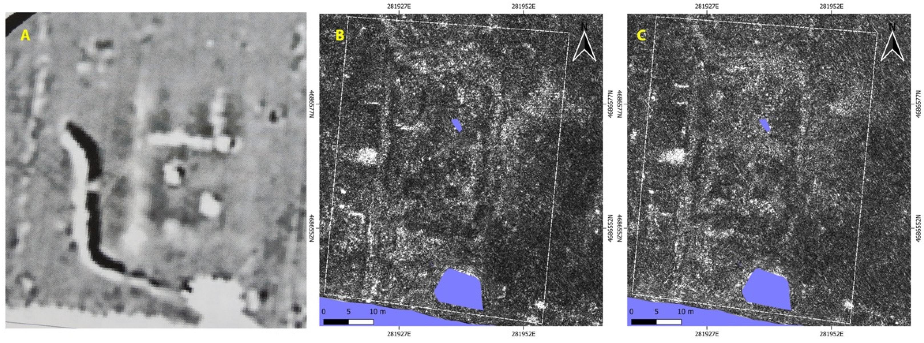
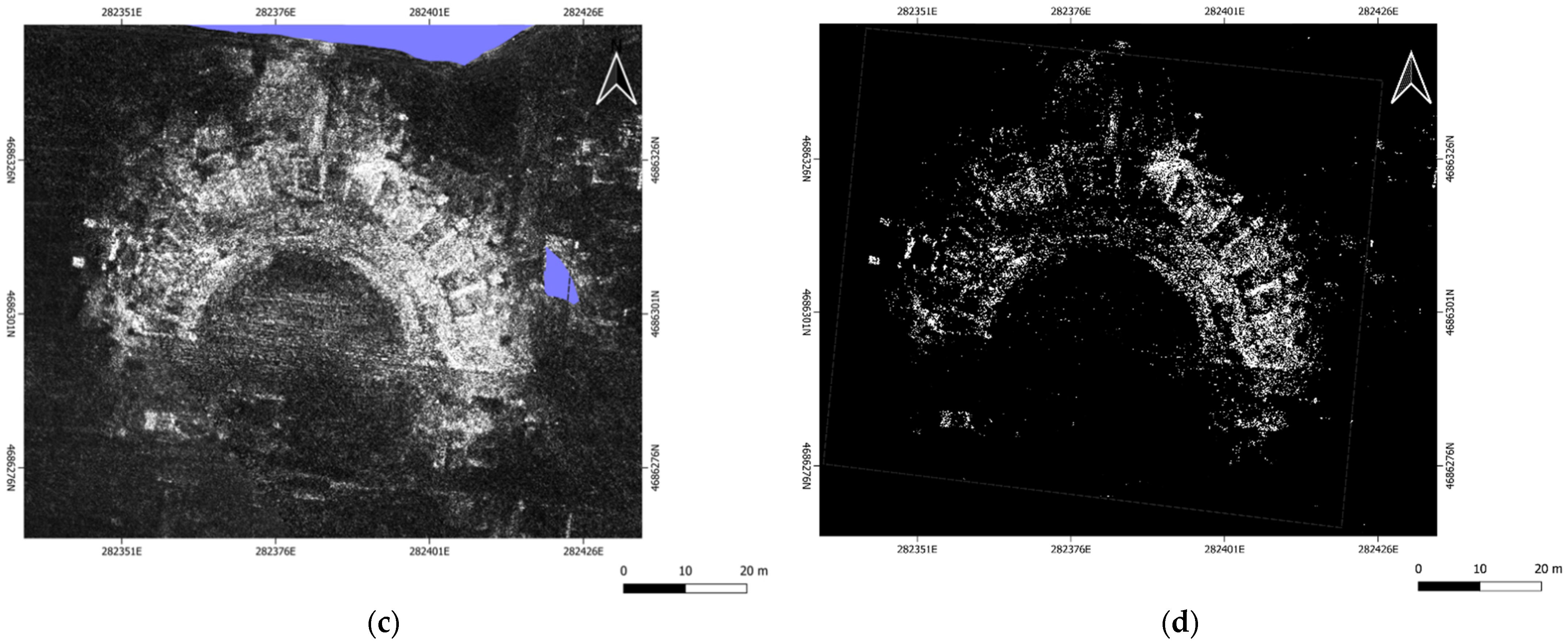
- In each new raster image produced in step 1, assign to the pixels the value of the estimated depth of the original time-slice. The result of this second step is a new raster image (that will be referred to as ‘signal peak slice’) where all pixels own the same depth value (Figure 1).
Figure 1 illustrates the differences between two time-slices and the corresponding “signal peak slice”.
The choice of a single pixel value or a range of values is related to the quality of time-slices and the degree of features visibility within them, which depends on the conditions, tools, and settings adopted in the phase of data acquisition and processing. As a general rule, the best combination of setting values can be determined, as a first step, by a preliminary study of the time-slice dataset (considered as a finite product of acquisition and processing procedures), as well as by an analysis of individual time-slices. As a second step, considering that the plug-in application requires little time, different settings can be tested to assess which one provides greater visibility and no data loss with respect to a single time-slice. For example, if by choosing a single peak value a loss of significant details and some weak buried object is observed when comparing the results to the single time-slices, it is recommended to change the setting and opt for a range of values. This solution certainly increases the background noise but can help not to miss details.
Both steps 1 and 2 are calculations performed by applying the QGIS raster calculator function. The GPR Raster pixel selection (step 1) and the assignation of the estimated depth from the ground (step 2) are expressed by the following equation:
where:
representing the “signal peak slice”, i.e., the final raster obtained from the processing of each GPR time-slice;
are the elements of a matrix representing the available GPR time-slice;
is the value of relative depth from the ground of each GPR time-slice;
may correspond to a single value or a range of values;
is the reference number of each processed GPR time-slice, maintained for the corresponding final raster produced.
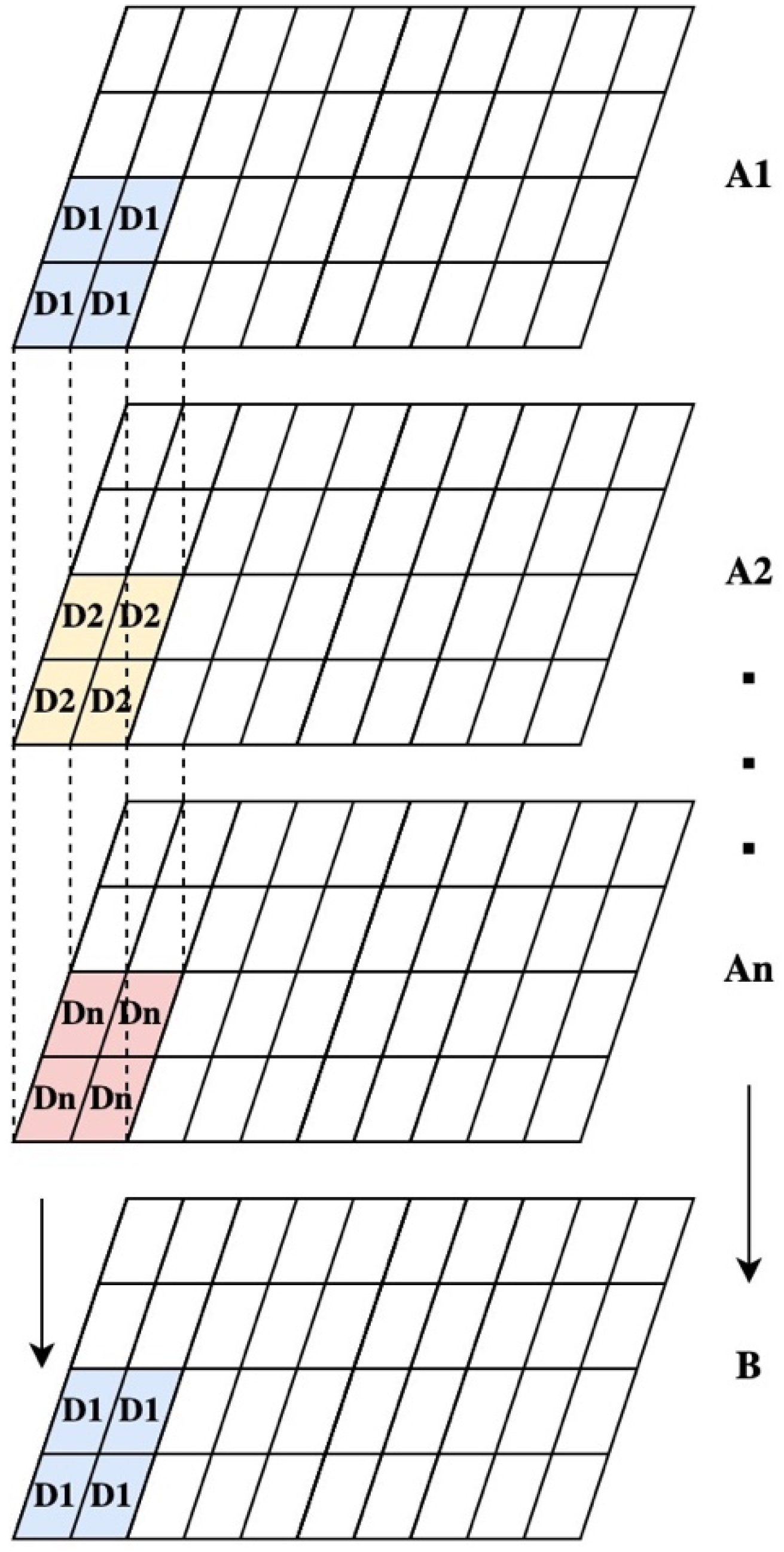
The second section of the automated process allows for merging “signal peak slices” (A) to produce a new single raster file, which maintains the value of the pixels contained in each “signal peak slice” processed, and in case of pixels overlapping, visualizes the pixel with the lower estimated depth value. The result of this step is a composite signal peak map (that will be referred to as “merged signal peaks map”) that allows a reading of the three-dimensional trend of subsurface structures and building rubbles, at the lower estimated depth they appear. Depth values can be visualized in a color scale by assigning a color to each depth considered. The amount of colors in the scale coincides with the number of time-slices reprocessed.
A GRASS [30] plug-in (r.series), which can be executed in QGIS, permits to run this raster merging operation of “signal peak slices” produced by the first automated process.
The following equation and Figure 2 show the raster merging process to produce the “merged signal peaks map” (B), where pixels indicate the lowest estimated depth at which structures and building rubble appear:
where:
B is the “merged signal peaks map”, i.e., the new raster with estimated depth pixel value produced by the merging process.
Figure 2.
Explanation diagram for overlapping values.
At this step, to amplify the results of this operation, the Inverse Distance Weighting (IDW) interpolation method (r.fill.stats) may be applied. The weighting value can be assigned and changed within the plug-in, by modifying both the interpolation distance threshold and the weighting coefficient, which both are set by default to two cells.
Following the merging process, by applying the open source modules GDAL (Geospatial Data Abstraction Library) [31], which facilitates the processing of geographic data in raster format, a null value is assigned to the cells resulting without depth information (gdal:fillnodata) and areas of interest may be selected by inserting a polygon that acts as a crop mask (gdal:cliprasterbymasklayer).
A further operation performed in the second section of the automated process consists in transforming the pixel values of estimated depth in absolute heights above sea level, which results in a new map (that will be referred to as “buried feature elevation map”). This operation is similar to the topographic correction that can be applied on GPR vertical profiles [3] (p. 121) [32,33]. To do so, a Digital Terrain Model (DTM) of the area is required, in order to calculate the difference between ground surface height and subsurface archaeological feature burial depth. This operation is done through the raster calculator in QGIS, as shown by the following equation:
where:
C = M − B
C is the “buried feature elevation map”, i.e., the final raster image with absolute height pixel values;
M is the DTM of the area.
As in the “merged signal peaks map” (B), pixel absolute height values in the “buried feature elevation map” (C) can be visualized in a color scale that allows a better reading of the buried structures and their state of conservation in elevation. Also, in this case, the amount of value/color of the scale coincides with the number of time-slices reprocessed. Elevation differences can be also visualized in sections by using already available QGIS plug-ins, such as Terrain Profile Tool, which allows visualizing the profile of subsurface features and building rubble in their relationship to the current ground surface.
Scheme 1 summarizes the whole automated procedure here explained.
2.2. Case Study and Dataset
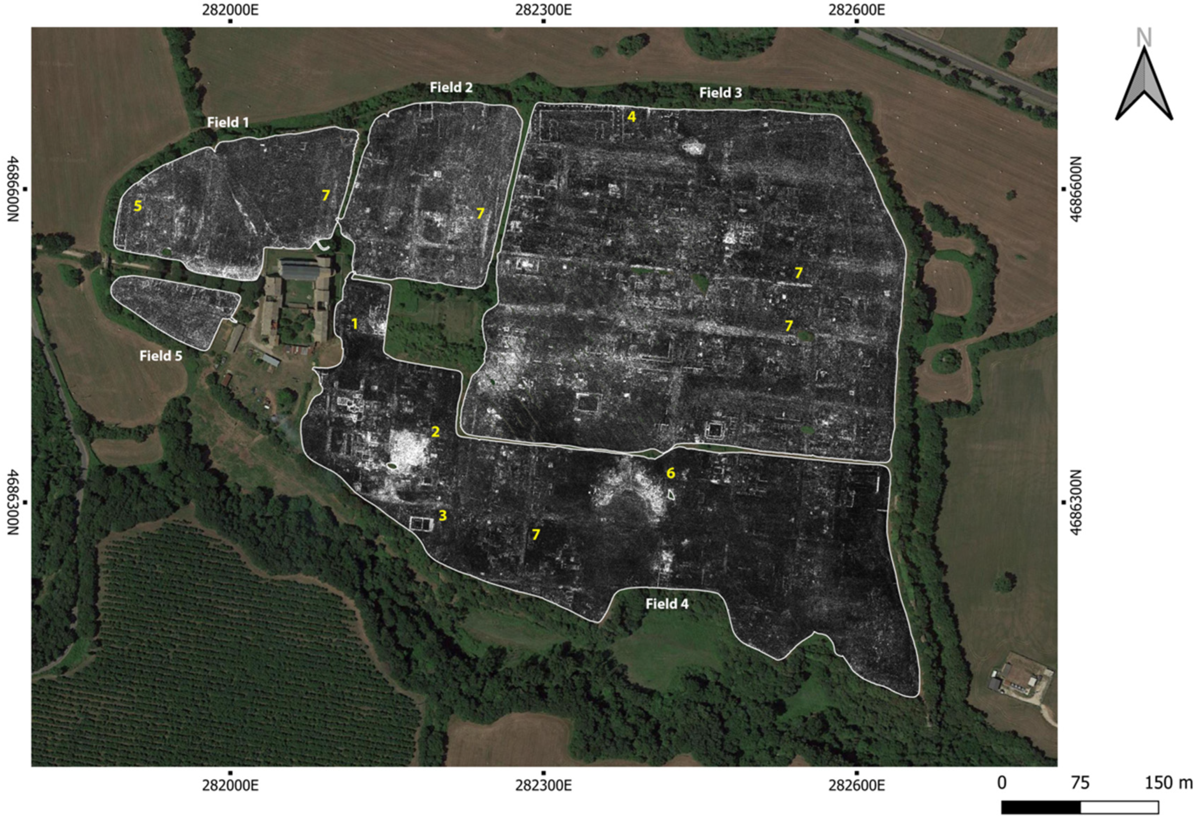
The Roman town of Falerii Novi is the first archaeological area selected to test the plug-in. Following the literary sources, the city was founded ex-novo in 241 BC, on a plateau characterized by a slight north-south slope, overlooking the gorge created by the stream of the Rio Purgatorio. The ancient urban walls, built-in large square tufa blocks, are still preserved in almost the whole perimeter, reaching at some points several meters in height. The Roman city lived up to the Early Middle Age. In a later phase, the Romanesque church of Santa Maria in Falleri and the annexed residential buildings were built above the level of the Roman buildings. Today, most of the Roman city lies almost completely underground, exception made for an area excavated in the second half of the last century and another small one inside the church. Nineteenth-century excavations investigated some other areas, which were after refilled in soil. Most of these are today difficult to locate, except the theater. The entire urban area underwent extensive geophysical survey, firstly by magnetometry [34], and recently with GPR [17,28] (Figure 3). The results of both surveys are high-quality data and allow for the reconstruction of the urban layout and the identification of several buildings.
The high-resolution GPR data produced by the Universities of Cambridge and Ghent [28], consists of time-slices at high resolution (5 cm per pixel), which show soil slices at a regular estimated depth interval of about 5 cm range, starting from the ground surface to 3 m deep. GPR data were acquired by 15,500 MHz antennae, arranged in two offset rows resulting in a vertical profile spacing of 0.125 m. A second pass was made to further reduce this spacing to 0.0625 m. The terrain vehicle was equipped with a global navigation satellite system receiver combined with a total station. Acquisitions were made only when the ground was sufficiently dry to yield optimal data quality and maintain interpretative potential, in order to always have a similar condition of the electrical conductivity of the soil. The processing of raw data to produce time-slices followed a standard workflow, which included background removal, further cleaning operations, and migration to improve lateral resolution [17] (p. 708 and Online Supplementary Material). The combination of high-standard acquisition tools and methods and raw data processing procedures produced high-quality time-slices. Data have been also analyzed by combining GPR results and the magnetic data available visualizing them in a single image by assigning the two datasets to different color channels (RGB compositing) [17] (pp. 714–716), and by investigating methods of computer-aided interpretation to create a 3D of structures [17] (p. 717), while manual mapping of anomalies in individual time-slices has also been adopted to compare and integrate the results of the computer-aided interpretation process [17] (p. 708).
The time-slices are available almost for the whole urban area, divided into five fields, whose limits are determined by surface conditions. The high resolution of the GPR data and the ability to indicate the depth of the features provide a much stronger foundation for understanding the town than before. Nevertheless, the results of the magnetometry and the GPR, when compared, appear profoundly different in many cases. On the one side, the GPR survey at Falerii Novi revealed many buildings previously unrecorded, such as a possible macellum (market building) ((1) in Figure 3), a bath complex ((2) in Figure 3), a temple surrounded by a portico ((3) in Figure 3), a porticus duplex ((4) in Figure 3), and a long rectangular portico with central raw of columns ((5) in Figure 3). In the case of other buildings, the GPR survey confirmed the results of the magnetic data, such as in the case of the theatre ((6) in Figure 3) and the alignment of several streets ((7) in Figure 3). Moreover, wherever the visibility of the detected features is higher, the high resolution of the GPR data and their ability to indicate features depth allowed to identify many individual structural elements (e.g., columns), as demonstrated by the temple surrounded by a portico ((3) in Figure 3), or in the case of the theatre ((6) in Figure 3). On the other side, GPR results are less clear than magnetic data in some parts of the urban area, for instance in many parts of field 5, about the rows of tabernae (shop units) in the forum square, which can be only partially seen, and the so-called porticus post scaena (porticoed area located south of the theatre), which is not visible at all.
This study has made use of the whole dataset of GPR georeferenced time-slices available for Falerii Novi, which has been imported in QGIS and processed following the steps illustrated in Section 2.1, firstly on the entire urban area, and then on a building scale. Considering that QGIS requires expressing the estimated depth with a unique value, this has been calculated by considering the two-way travel time indicated in each time-slice and the average subsurface wave velocity of each field, as indicated in [28] (csv-files). Once obtained an estimated depth range, an average value has been calculated and adopted (see example Figure 1).
An available DTM of the urban area at 10 cm pixel resolution, produced by the University of Tuscia in 2017, has been used in the final step of the procedure to calculate the absolute height of the features detected. Field data were acquired by using a drone (Phantom 4 Pro) and post-processed by adopting open-source software for image processing and georeferencing (Open Drone Map) [35]. The high-resolution DSM (Digital Surface Model) of the area produced, has been then transformed into a DTM, after being calibrated with GNSS points. Even if the DTM has a lower resolution than the GPR data, its use has been determined by the fact that field data has been collected in a period close to the GPR data acquisition (2015–2017).
The coordinate system used for all the georeferenced images in this article is EPSG: 32633-WGS 84/UTM zone 33N.
3. Results
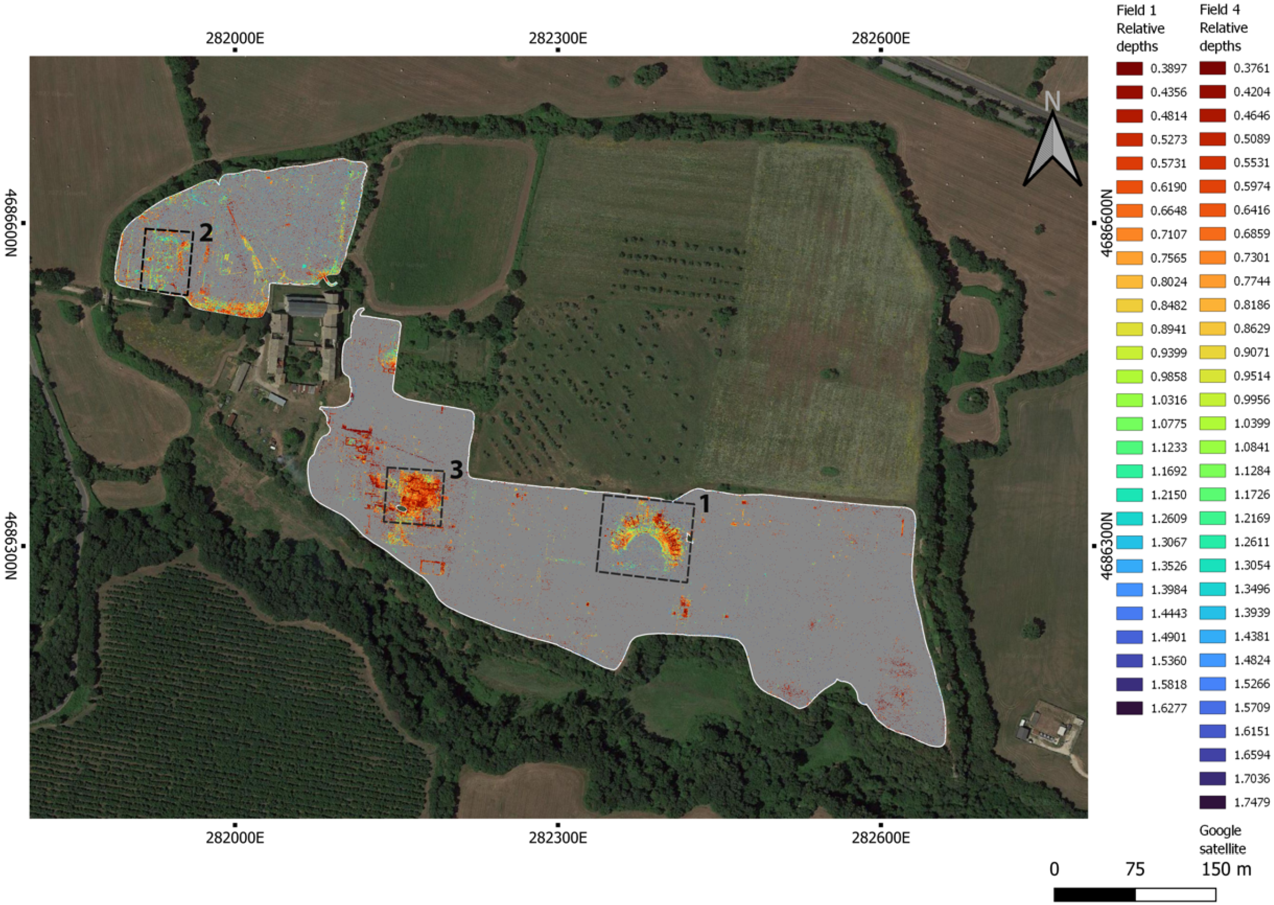
As a first step, the whole Falerii Novi dataset of time-slices was analyzed and the depth range was identified at which archaeological features are visible in each field, as can change case by case. Once established the depth range of interest, the selected time-slices have been processed following the steps described in Section 2.1. Figure 4 shows the “merged signal peaks map” (B) of fields 1 and 4, including time-slices at estimated depths from about 0.37 to 1.75 m. The peak value in the original time-slices has been recognized in pixel color value 255. Considering the high quality of this dataset, it was possible to identify a single value instead of a range of values.
A second phase of the test concerned smaller areas, leading the analysis at a building scale. The buildings selected are the theater ((1) in Figure 4), the “Capitolium” (temple) ((2) in Figure 4), and a bath complex ((3) in Figure 4). The areas of interest have been cut from the “merged signal peaks maps”, and “buried feature elevation maps” have been produced. To increase the visibility of depth/elevation differences, an RGB color scale is chosen for the B and C maps. The order of colors is maintained consistently in all products, indicating in red the values corresponding to the lowest depth/higher height, in green values near the middle of the scale, and in blue the higher depth/lower elevation values. The amount of value/color in the scale corresponds to the number of reprocessed time-slices. The results of these tests are illustrated and firstly discussed in the following Sections.
3.1. The Theater
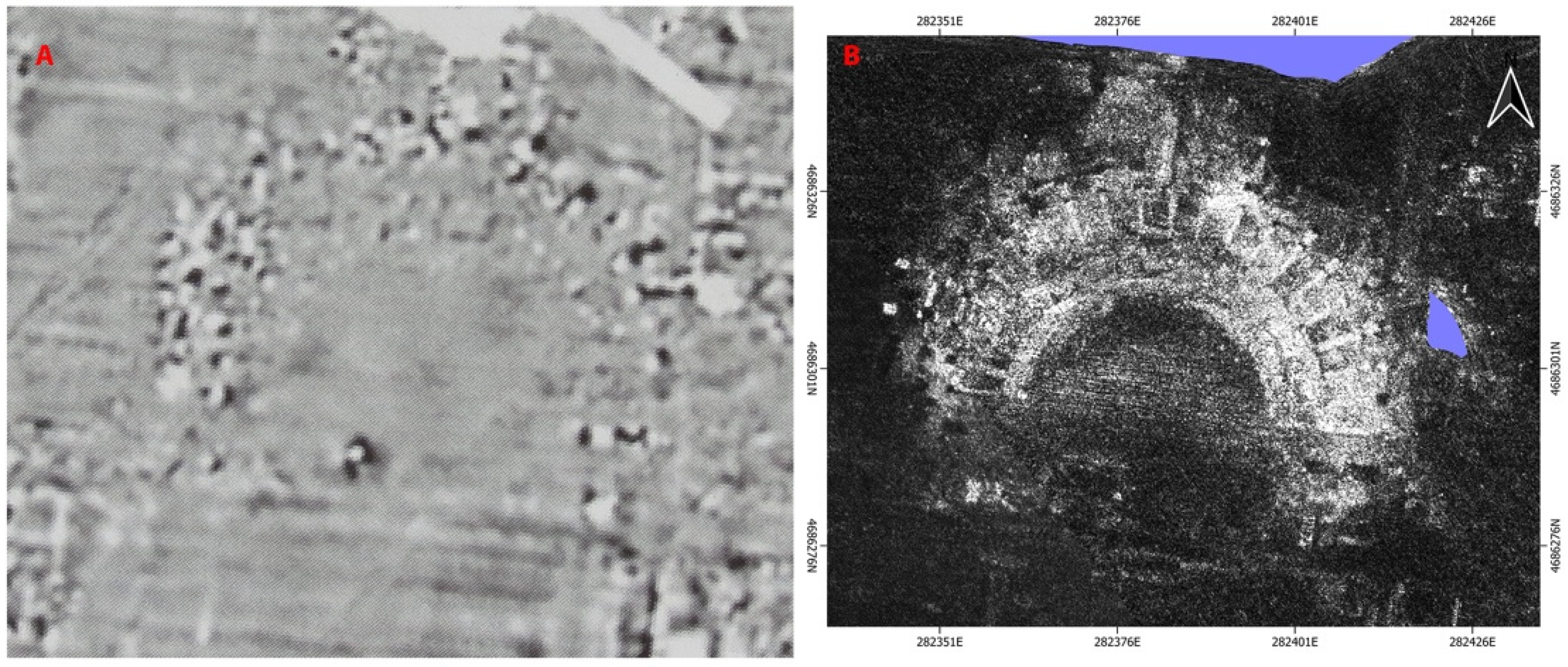
The theater is located south of the forum. The incorrect placement of the nineteenth-century excavations [36], combined with the small detail of the magnetometry results, prevented the exact definition of the perimeter of the building [34] (pp. 75–79). On the contrary, the GPR survey gives an extremely clear image of the structure (Figure 5).
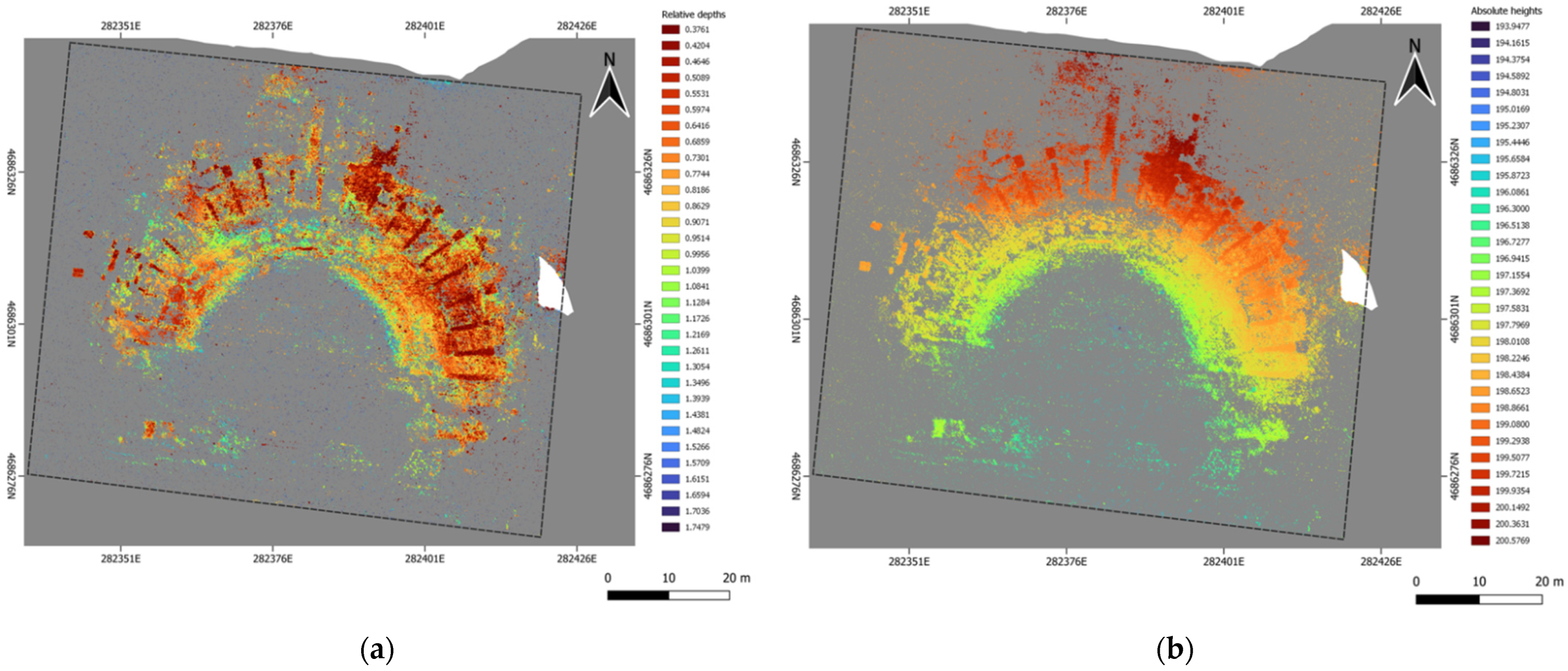
Figure 6 shows the results of the plug-in application on the GPR data, selecting a series of 32 time-slices from the one between 8–9 ns to the one between 39–40 ns, since the structural elements composing the theatre are visible within this range of horizontal profiles. Interpolation was performed with one cell. The results produced are the “merged signal peaks map” with estimated depth pixel values (Figure 6a), and the “buried feature elevation map” with absolute heights (Figure 6b).
The maps produced show the radial walls supporting the summa cavea (upper seat steps), the steps of the ima cavea (lower seat steps) and the perimeter of the orchestra, found at a lower height. The scaenae frons (stage and stage architectural background) is also visible, characterized by three apsidal niches, of which the central one may be wider. This is the less evident part of the building, possibly because less preserved. All these features were already visible in the original time-slices, nevertheless, the results achieved by the merging process allow a synchronic view of different depth points. Moreover, transforming depth values into absolute heights permits one to fully appreciate the specific architectonic nature of the theatre, characterized by the combination of structural elements located at different heights, and to put in evidence their state of conservation. About this, the “buried feature elevation map”, because of the information it gives as a synchronic view of time-slices, provides an effective and functional resource for the analysis of the building, which can be also used as a base for future 3D reconstruction.
The result achieved also allows us to make a further observation concerning some parts of the building remains where a low concentration of building rubble is visible, in particular between the radial walls supporting the summa cavea in its western portion, while in the other parts they appear as filled and covered in building rubble. This western part of the theater corresponds to the one that underwent excavations in 1823 when building rubble was possibly removed to uncover structures. This excavation area is recorded in the map of the ancient city drawn in 1831 by Vespignani (, who also included the eastern area of the theater, excavated in 1829 [36]. Since the “buried feature elevation map” shows in the latter area the broad presence of building rubble among the walls of the summa cavea, it can be hypothesized that those excavation activities interested only the most superficial portion of the stratigraphy.
3.2. The “Capitolium”
At the north-western end of the urban area, at its highest point (today at about 210 m a.s.l.), a major structure (c 23 × 34 m long, aligned north-south) was identified by the magnetometer survey and interpreted as a large temple with a possible tripartite cell (with back wall undetected). Because of this latter characteristic and the elevated location within the town, the temple was referred to as capitolium [34] (p. 11). On the contrary, in the single GPR time-slices which offer the best visibility, the configuration of the temple is less evident, such for instance the tripartition of the cell (Figure 7). For this reason, the “Capitolium” was selected for testing the plug-in and to see if the final results of the automated process could put in evidence anomalies that can be interpreted as architectural features, difficult to identify by manual interpretation and mapping of each separate time-slice.
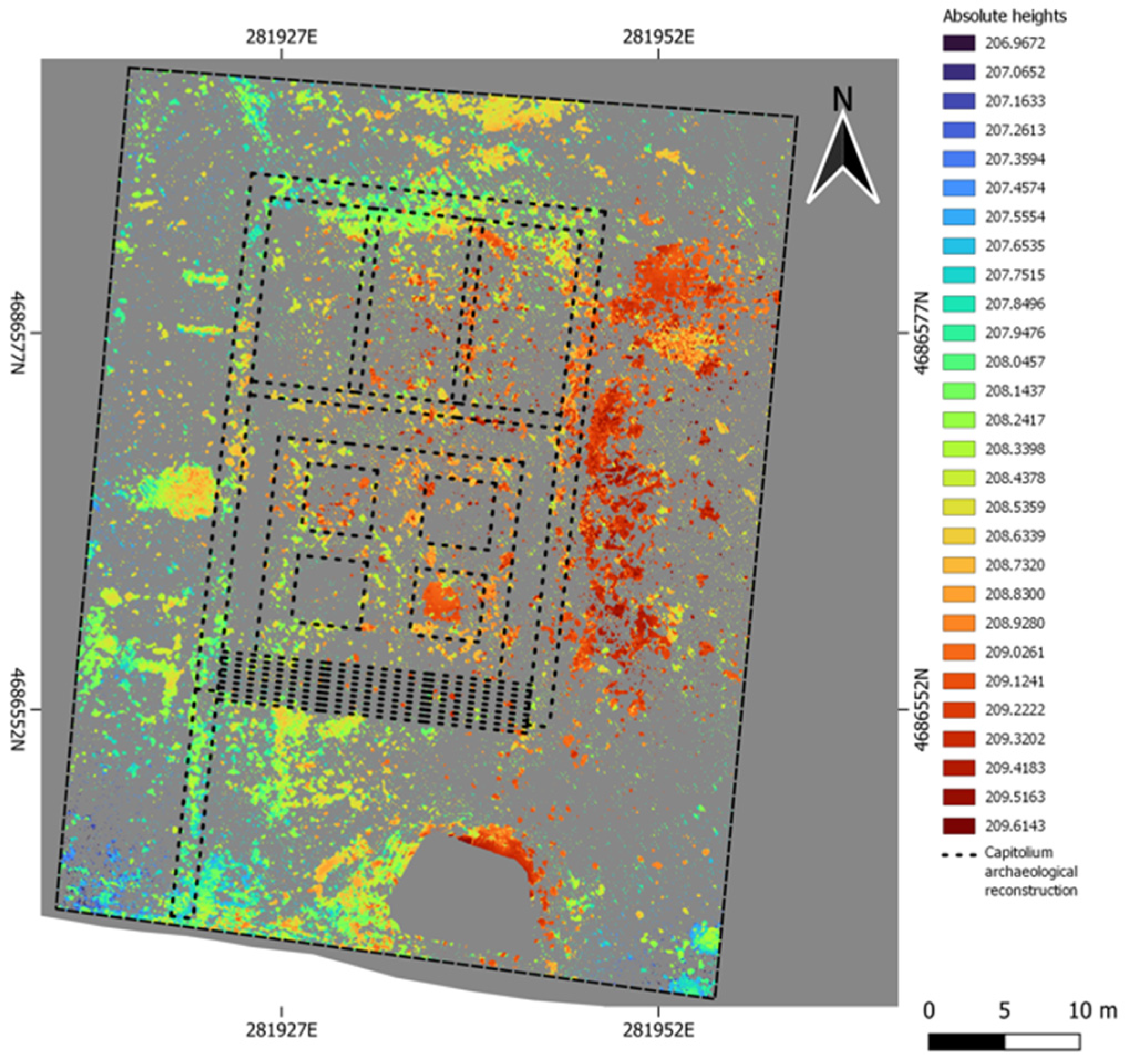
Figure 8 shows the results of the plug-in application on the GPR data, selecting a series of 28 time-slices from the one between 8–9 ns to the one between 35–36 ns, since the structural elements composing the “Capitolium” are visible within this range of horizontal profiles. The interpolation values have been left at default two cells. The results produced are the “merged signal peaks map” with estimated depth pixel values (Figure 8a), and the “buried feature elevation map” with absolute heights (Figure 8b).
Results confirm the presence of a temple with a tripartite cell, as already identified by the magnetometer survey. In addition, the results of the plug-in application show well the presence of the northern wall of the tripartite cell, as well as a regular wall pattern in front of the cell, which may be interpreted as a crawl space functioning as a substructure of the floor and a three row colonnade. In front of this, further south, the “buried features elevation map” (Figure 8a) suggests the presence of steps that could have connected the temple with a terrace or square located at a lower level and facing the main east-west road. Moreover, the levels at which other structures surrounding the temple are located suggest that it was on a podium (Figure 9).
3.3. The Bath Complex
The GPR survey identified for the first time a large building complex in the central-southern area of the city. This ensemble of adjacent rooms of different sizes and shapes has been realistically interpreted as a bath complex [17]. This is also one of the few building complexes already described in a paper by the survey authors, which applied a computer-aided procedure to detect walls and floors [17] (Figure 9c), thus offering a clear and detailed reconstruction of the preserved structural elements.
In the light of the observations done in the cases of the “Capitolium” and the theater about the plug-in contribution for the visualization of the absolute height of structures, this building complex has been selected to verify if the plug-in application may help to better understand the plan of this building, and, in particular, to visualize possible differences in elevation among its various parts.
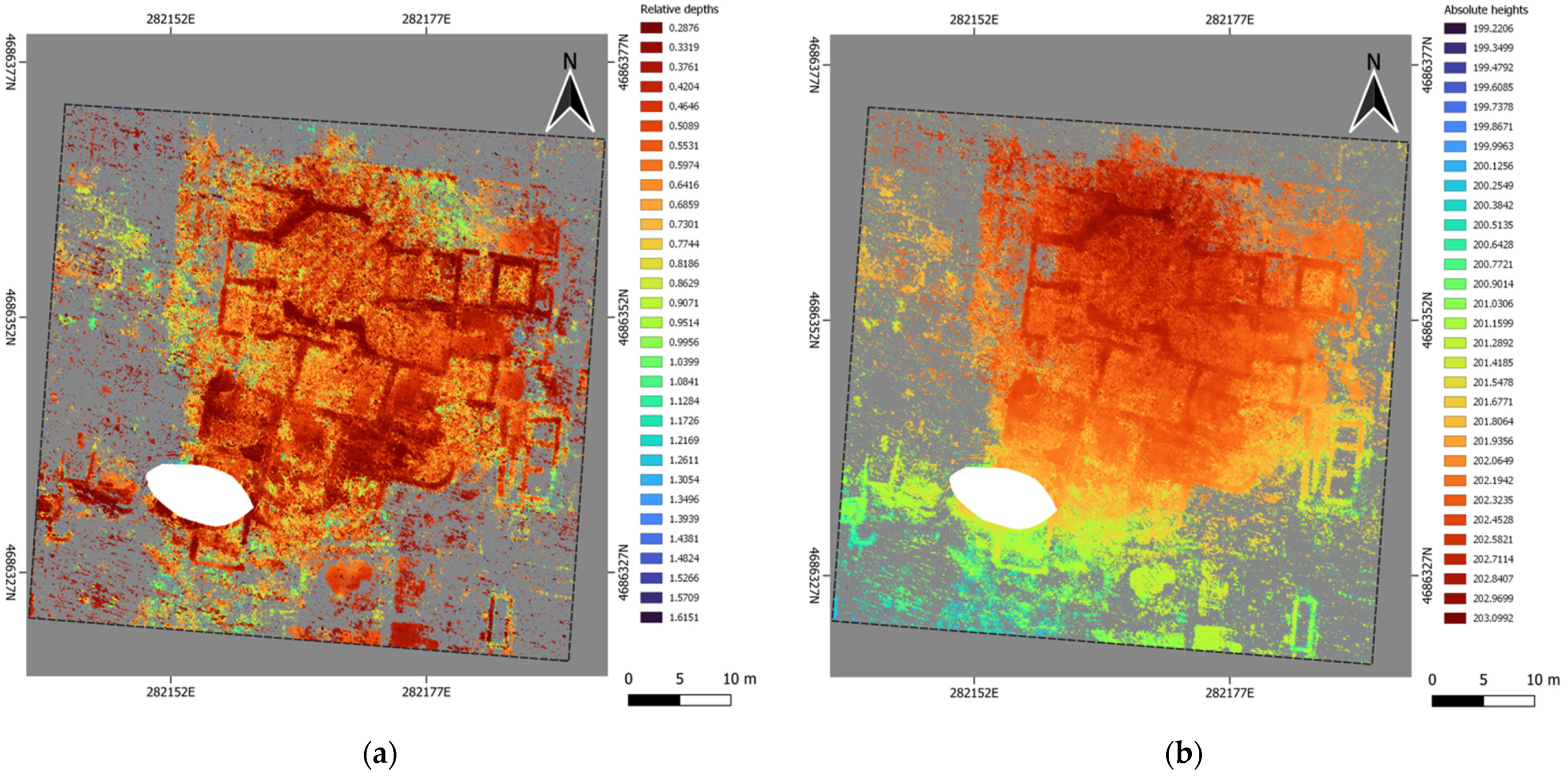
Figure 10 shows the results of the plug-in application on the GPR data, selecting a series of 31 time-slices from the one between 6–7 ns to the one between 36–37 ns, since the structural elements composing the baths, especially walls, are preserved closer to the soil surface in this area. In this case, the interpolation values are set at 1 cell instead of the default 2 cells, because the high presence of building rubbles already disturbs the visibility of deeper structures. The results produced are the “merged signal peaks map” with estimated depth pixel values (Figure 10a), and the “buried feature elevation map” with absolute heights (Figure 10b).
Concerning the building plan, the results mostly confirm the ones achieved by the computer-aided detection of anomalies in the original GPR data [17] (Figure 9). Some differences concern walls. In the case of the octagonal room, walls look more defined after the plug-in processing, while, conversely, in other parts of the complex some walls do not appear at all or are less defined, possibly because they are hidden by most superficial stratigraphy. A similar observation concerns floors, which do not appear clearly both in the “merged signal peaks map” and in the “buried feature elevation map”, while they were identified by computer-aided detection, which made use of GPR vertical sections [17] (p. 715), which cannot be processed by the plug-in.
Nevertheless, by observing the “buried feature elevation map” (Figure 10b), an evident difference in height is registered along the north-south street running west of the building. The “buried feature elevation map” shows that the street descended toward the south from an estimated height of 202 to 200.5 m ca. in 48 m distance, highlighting a topographic difference of about 1.50 m and a slope of 3%. In light of this, a more careful analysis of absolute heights pixel values has been carried out within the building complex. It allowed glimpsing below the level of rubble two possible more homogeneous levels, possibly corresponding to floors. The first is in the octagonal room and the surrounding ones at about 202 m in height, and the second is in the rooms located further south at about 201.5 m. These considerations may suggest that rooms were located at slightly different levels as descending toward the south to compensate for the difference in terrain height.
4. Discussions
The developed plug-in is a user-friendly tool, whose main benefit is its capacity to automatically extract subsurface features out of GPR time-slices in QGIS and to visualize them in a single image. As explained, the tool was firstly developed in the context of soil erosion risk assessment to create a model of the upper surface of the archaeological deposit, but this pixel-based approach and the possibility to analyze a higher number of time-slices as raster input data, suggested further exploration of the opportunity to use it to automatically input evidence features of archaeological interest within time-slices in a quick and efficient way. Furthermore, the plug-in was designed so that the user can decide the series of time-slices to process (up to 60 units), and change the settings with respect to peak pixel values and interpolation values.
In terms of archaeological knowledge, the plug-in facilitates the process of interpretation of subsurface archaeological structures, as the two types of maps produced offer different types of information. Because of this, the “merged signal peak map” should not be considered as an intermediate product to obtain the “buried features elevation map”, but rather as an independent result. In fact, the “merged signal peak map”, since it clearly shows the estimated distance from the surface of archaeological structures, as well as the presence and extension of building rubble, can be a useful and expeditious tool for the planning and execution of excavation activities. This can provide helpful information while deciding if, where, and how to use mechanical equipment or manual soil removal, especially in the most superficial layers. On its side, the “buried feature elevation map” is suitable to emphasize and better appreciate the three-dimensional configuration of buildings. This is more evident in the two-dimensional rendering of the theater, nonetheless, in the case of the “Capitolium” the C map even permitted the recognition of specific characteristics of the structure, such as that the temple structure was probably built on a podium, as highlighted by the different heights of the temple remains and the surroundings. Obviously, the two maps will be similar in a flat area, while, in the case of a slope, it can be noted that the “buried features elevation map” offers a more realistic image of structures in their three-dimensional development than the “merged signal peak map”.
Since the plug-in produces a 3D visualization, it offers an intermediate solution between a two-dimensional map and a 3D model. With respect to other manual mapping of anomalies through GIS tools, the plug-in process is automatic, thus faster and less prone to subjectivity. In this sense, the maps offer information that is not usually obtained in GIS, while they are more similar to the ones obtained by using 3D modeling tools, which, however, are usually proprietary software and require several steps.
Besides the benefits, the two-dimensionality of plug-in products is also its most evident limit in terms of building visualization and related interpretation. This is because, as explained, the merging procedure permits only one value to be visualized in each pixel, therefore, in case of values overlapping, only the more superficial ones are taken while the deeper ones are eliminated (Equation (2)). Because of this, features covered, for example, by building rubbles could be less visible or not recorded in the final maps, such as walls and particularly floors, as seen in the case of the bath complex. This implies that the 3D visualization achieved on a raster base should be then further developed by moving to a vector representation, in order to build a 3D model. Nevertheless, the plug-in, at the current state of software development, is already capable of managing large datasets of GPR time-slices and providing products useful for the interpretation of subsurface structures, as demonstrated by the results of the case studies considered.
However, it must be noticed that, since the plug-in does not work on GPR raw data but on time-slices made in a phase and with procedures entirely independent from the tool, any inaccuracies in the time-slices affect the final products. In this regard, if a topographic correction has been applied or not, or an average value of soil permittivity and pulse velocity has been chosen instead of punctual values, this can affect the topographic margin of error of the maps. For instance, if the actual pulse velocity is locally lower than the average value used during GPR data acquisition, the features will appear in the time-slices at a greater depth than the one at which they actually are placed, and this, in turn, will create differential changes in the geospatial position of the pixel in the “merged signal peaks map”. The same applies to the accuracy of the DTM used for the generation of the “buried feature elevation map”.
5. Conclusions
In this paper, the results of the plug-in test on Falerii Novi GPR time-slices have been illustrated in order to give a first report of the plug-in application potential. Nevertheless, the test phase is not yet concluded and the plug-in is still not published as a software. Before publishing it as an open source software, further development phases are already planned. Tests on other GPR datasets have to be completed, so that the study may also focus on the effectiveness of the plug-in with respect to datasets at different resolutions, acquired with different tools and pedological conditions, and time-slices pre-processed by using different tools and methods. Moreover, since a more robust interpretation of the subsoil can be achieved by combining different types of geophysical data, it would be interesting to carry out further tests of the plug-in on horizontal depth-slices generated by combining different geophysical datasets three-dimensional in nature (such as GPR data and electrical imaging). Finally, the research is already addressing the exploration of opportunities to use the same pixel-based approach of the procedure here illustrated as a base for the creation of vectorial 3D models of buildings and other types of structures, which will permit the overlapping issue to be overcome. The challenge is to automatically create and visualize point clouds of GPR anomalies, also by using basic support for the management and visualization of 3D datasets in an open source GIS environment, which will permit volumes pertaining to coherent structures (walls and floors) to be distinguished and 3D models of buildings to be created.
Author Contributions
Conceptualization, S.D.A., M.S. and F.B.; methodology, S.D.A., M.S. and F.B.; software, M.S.; validation, M.S., S.D.A. and F.B.; formal analysis, S.D.A., M.S. and F.B.; investigation, M.S., S.D.A. and F.B.; data curation, M.S.; writing—original draft preparation, F.B.; writing—review and editing, S.D.A., F.B. and M.S.; visualization, M.S.; supervision, S.D.A. and F.B.; project administration, S.D.A.; funding acquisition, S.D.A. All authors have read and agreed to the published version of the manuscript.
Funding
This study was funded by project RESEARCH, which has received funding from the European Union’s Horizon 2020 research and innovation programme under the Marie Skłodowska-Curie grant agreement No. 823987.
Acknowledgments
We thank the authors of the GPR survey activity in Falerii Novi for having made available the GPR data of Falerii Novi in open access, and particularly Martin Millett for the permission of reproducing the image of the magnetometry survey in Falerii Novi from PBSR. Other thanks go to Philip Fayad, for his substantial contribution in the first phase of software development, Roberto Montagnetti for the realization of the DTM used in data processing, and Luna Battistin and Konstantinos Fokeas for a review of the equations. Thanks also to the five anonymous referees and the editors for the constructive criticism of an earlier draft of this article.
Conflicts of Interest
The authors declare no conflict of interest.
References
- Conyers, L.B.; Goodman, D. Ground Penetrating Radar. In An Introduction for Archaeology; AltaMira Press: Walnut Creek, CA, USA; London, UK; New Delhi, India, 1997; ISBN 978-0761989288. [Google Scholar]
- Conyers, L.B. Ground-Penetrating Radar for Archaeology, 3rd ed.; Rowman and Littlefield: Lantham, MD, USA, 2013; ISBN 978-0759123489. [Google Scholar]
- Goodman, D.; Piro, S. GPR Remote Sensing in Archaeology; Springer: Heidelberg, Germany; New York, NY, USA; Dordrecht, The Netherlands; London, UK, 2013; ISBN 978-3-642-31857-3. [Google Scholar]
- Conyers, L.B. Ground-Penetrating Radar and Magnetometry for Buried Landscape Analysis; Springer: Heidelberg, Germany; New York, NY, USA; Dordrecht, The Netherlands; London, UK, 2018; ISBN 978-3-319-70890-4. [Google Scholar]
- Conyers, L.B.; Martínez, A. Georadar Aplicado en Geotecnia y Arqueología; GeoMantis: Monterrey, Mexico, 2021; ISBN 978-1-63972-317-1. [Google Scholar]
- Pérez, G.V.; Caselles, J.O.; Clapés, J.; Osorio, R.; Martínez, G.; Canas, J.A. Integrated near- surface geophysical survey of the Cathedral of Mallorca. J. Archaeol. Sci. 2009, 36, 1289–1299. [Google Scholar] [CrossRef]
- Gabellone, F.G.; Leucci, G.; Masini, N.; Persico, R.; Quarta, G.; Grasso, F. Nondestructive prospecting and virtual reconstruction of the chapel of the Holy Spirit in Lecce, Italy. Near Surface Geophys. 2013, 11, 231–238. [Google Scholar] [CrossRef]
- Lampropoulos, K.C.; Moropoulou, A.; Korres, M. Ground penetrating radar prospection of the construction phases of the Holy Aedicula of the Church of the Holy Sepulchre, in correlation with architectural analysis. Constr. Build. Mater. 2017, 155, 307–322. [Google Scholar] [CrossRef]
- Benedetto, A.; Pajewski, L. (Eds.) Civil Engineering Applications of Ground Penetrating Radar. In Springer Transactions in Civil and Environmental Engineering; Springer: Cham, Switzerland, 2015. [Google Scholar]
- Solla, M.; Pérez-Gracia, V.P.; Fontul, S. A review of GPR application on transport infrastructures: Troubleshooting and best practices. Rem. Sens. 2021, 13, 672. [Google Scholar] [CrossRef]
- Li, S.; Gu, X.; Xu, X.; Xu, D.; Zhang, T.; Liu, Z.; Dong, Q. Detection of concealed cracks from ground penetrating radar images based on deep learning algorithm. Construct. Build. Mater. 2021, 273, 121949. [Google Scholar] [CrossRef]
- Rasol, M.; Pais, J.C.; Pérez-Gracia, V.; Solla, M.; Fernandes, F.M.; Fontul, S.; Ayala-Cabrera, D.; Schmidt, F.; Assadollahi, H. GPR monitoring for road transport infrastructure: A systematic review and machine learning insights. Construct. Build. Mater. 2022, 324, 126686. [Google Scholar] [CrossRef]
- Wunderlich, T. MultichannelGPR—A New MATLAB-Tool for the Processing of GPR Data. ArcheoSciences 2021, 45, 279–283. [Google Scholar] [CrossRef]
- Nuzzo, L.; Leucci, G.; Negri, S.; Carrozzo, M.T.; Quarta, T. Application of 3D visualization techniques in the analysis of GPR data for archaeology. Ann. Geophys. 2002, 45, 321–337. [Google Scholar] [CrossRef]
- Leckebusch, J.; Weibel, A.; Bühler, F. Semi-automatic feature extraction from GPR data for archaeology. Near Surf. Geophys. 2008, 6, 75–84. [Google Scholar] [CrossRef]
- Küçükdemirci, M.; Sarris, A. Deep learning based automated analysis of archaeo-geophysical images. Archaeol. Prospect. 2020, 27, 107–118. [Google Scholar] [CrossRef]
- Verdonck, L.; Launaro, A.; Vermeulen, F.; Millett, M. Ground-penetrating radar survey at Falerii Novi: A new approach to the study of Roman cities. Antiquity 2020, 94, 705–723. [Google Scholar] [CrossRef]
- Bornik, A.; Neubauer, W. 3D Visualization Techniques for Analysis and Archaeological Interpretation of GPR Data. Remote Sens. 2022, 14, 1709. [Google Scholar] [CrossRef]
- Watters, M.S. Geovisualization: An Example from the Catholme Ceremonial Complex. Archaeol. Prospect. 2006, 13, 282–290. [Google Scholar] [CrossRef]
- Deiana, R.; Bonetto, J.; Mazzariol, A. Integrated Electrical Resistivity Tomography and Ground Penetrating Radar Measurements Applied to Tomb Detection. Surv. Geophys 2018, 39, 1081–1105. [Google Scholar] [CrossRef]
- Kelly, T.B.; Angel, M.N.; O’Connor, D.E.; Huff, C.C.; Morris, L.E.; Wach, G.D. A novel approach to 3D modelling ground-penetrating radar (GPR) data—A case study of a cemetery and applications for criminal investigation. Forensic Sci. Int. 2021, 325, 1–15. [Google Scholar] [CrossRef] [PubMed]
- Ogden, J.; Strutt, K.; Keay, S.; Earl, G.; Kay, S. Geophysical prospection at Portus: An evaluation of an integrated approach to interpreting subsurface archaeological features. In Proceedings of the 37th Computer Applications to Archaeology Conference (CAA 2009), Williamsburg, VA, USA, 22–26 March 2009; Frischer, B., Webb, C.J., Koller, D., Eds.; Colonial Williamsburg Foundation: Williamsburg, VA, USA, 2010; pp. 1–17. [Google Scholar]
- De Angeli, S.; Battistin, F.; Serpetti, M.; Di Iorio, A.; Moresi, F.V. The RESEARCH project, Soil-related hazards and archaeological heritage in the challenge of Climate Change. In Proceedings of the Florence Heri-Tech 2020, the Future of Heritage Science and Technologies, IOP Conference Series, Materials Science and Engineering, Online, 14–16 October 2020. [Google Scholar] [CrossRef]
- De Angeli, S.; Battistin, F.; Moresi, F.V.; Fayad, P.; Serpetti, M. Valutazione integrata delle dinamiche di rischio di erosione del suolo in presenza di depositi archeologici. II metodo proposto dal progetto RESEARCH (REmote SEnsing techniques for ARCHaeology). In ARCHEOFOSS XIV 2020; Bogdani, J., Montalbano, R., Rosati, P., Eds.; Archeopress: Oxford, UK, 2021; pp. 13–23. ISBN 978-1-80327-125-5. [Google Scholar]
- De Angeli, S.; Serpetti, M.; Fayad, P.; Battistin, F. An Open-Source Approach for the Vulnerability Assessment of Archaeological Deposits Using Gpr Data in Qgis Environment. In Proceedings of the CAA2021, Digital Crossroads, Online, 14–18 June 2021. [Google Scholar]
- QGIS Geographic Information System. QGIS Association. 2022. Available online: http://www.qgis.org (accessed on 12 May 2022).
- QGIS 3.22. Geographic Information System Developers Manual. QGIS Association. 2022. Available online: https://docs.qgis.org/3.22/en/docs/developers_guide/index.html (accessed on 12 May 2022).
- Millett, M.; Verdonck, L.; Leone, N.; Launaro, A. Beneath the surface of Roman Republican cities (dataset). Archaeol. Data Serv. 2019, 59–61. [Google Scholar] [CrossRef]
- Schmidt, A.; Ernenwein, E. Guide to Good Practice: Geophysical Data in Archaeology, 2nd ed.; Archaeology Data Service; Available online: https://guides.archaeologydataservice.ac.uk/g2gp/Geophysics_Toc (accessed on 14 May 2022).
- GRASS-PROJECT. Geographic Resource Analysis Support System. 2013. Available online: https://grass.osgeo.org (accessed on 12 May 2022).
- GDAL-SOFTWARE-SUITE. Geospatial Data Abstraction Library. 2013. Available online: https://gdal.org (accessed on 12 May 2022).
- Prokhorenko, V.; Ivashchuk, V.; Korsun, S.; Musiyachenko, S.; Borodavka, V. Topographic correction of GPR profile based on odometer and inclinometer data. In Proceedings of the 2012 14th International Conference on Ground Penetrating Radar (GPR), Shanghai, China, 4–8 June 2012; pp. 425–429. [Google Scholar] [CrossRef]
- Zhang, D.; Zhong, R.; Li, J.; Zeng, F. Topographic Correction of GPR Profiles Based on Laser Data. In Proceedings of the 35th International Symposium on Remote Sensing of Environment (ISRSE35), Beijing, China, 22–26 April 2013; Volume 17, p. 012251. [Google Scholar] [CrossRef]
- Keay, S.J.; Millett, M.; Poppy, S.; Robinson, J.; Taylor, J.; Terrenato, N. Falerii Novi: A new survey of the walled area. Pap. Br. Sch. Rome 2000, 68, 1–93. [Google Scholar] [CrossRef]
- OpenDroneMap. A command line toolkit to generate maps, point clouds, 3D models and DEMs from drone, balloon or kite images. OpenDroneMap/ODM GitHub Page. 2020. Available online: https://github.com/OpenDroneMap/ODM (accessed on 14 May 2022).
- Di Stefano Manzella, I. Falerii Novi Negli Scavi Degli Anni 1821–1830; L’Erma Di Bretschneider: Roma, Italy, 1979; Volume 1821–1830, pp. 1–188. ISBN 9788870622508. [Google Scholar]
Figure 1.
Comparison between time-slices (T) and related “signal peak slices” (A) from the Falerii Novi dataset: (a) Field 4, time-slice 07–08 ns (estimated depth 0.3097–0.3540 m) [28]; (b) “signal peak slice” obtained from the processing of a on the base of pixel value 255, to which is assigned an average depth value of 0.3318 m (image by M. Serpetti); (c) Field 4, time-slice 17–18 ns (estimated depth 0.7522–0.7965 m) [28]; (d) “signal peak slice” obtained from the processing of c on the base of pixel value 255, to which is assigned an average depth value of 0.7743 m (image by M. Serpetti).
Scheme 1.
Flowchart of the plug-ins processing chain.
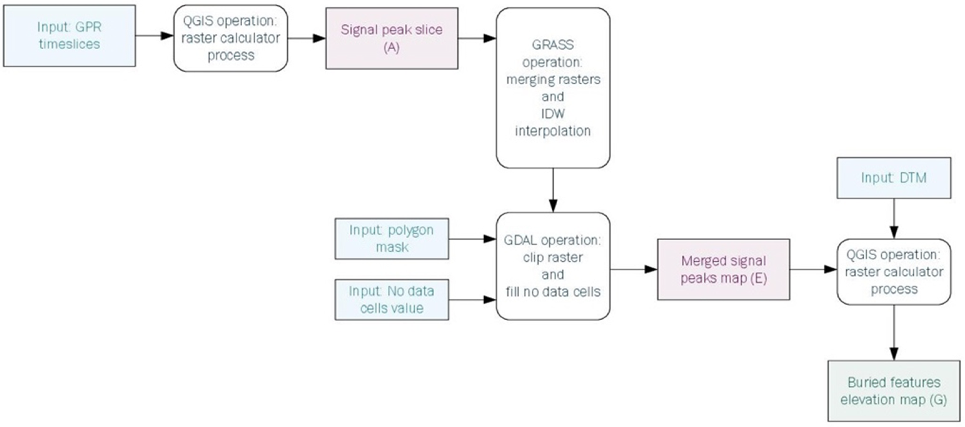
Figure 3.
Falerii Novi, urban area. GPR time-slice between 14–15 ns of fields 1, 2, 3, 4, and 5. Numbers indicate: (1) the “macellum”; (2) bath complex; (3) temple; (4) porticus duplex; (5) columned portico; (6) the theatre; (7) streets (time-slices from [28]; aerial photograph from Google Earth; image by M. Serpetti).

Figure 4.
Falerii Novi, “merged signal peaks map” of fields 1 (time-slices from 8–9 to 35–36 ns) and 4 (time-slices from 8–9 to 39–40 ns), and indication of case study areas: (1) the theatre; (2) the “Capitolium”; (3) the bath complex (aerial photograph from Google Earth; image by M. Serpetti).
Figure 4.
Falerii Novi, “merged signal peaks map” of fields 1 (time-slices from 8–9 to 35–36 ns) and 4 (time-slices from 8–9 to 39–40 ns), and indication of case study areas: (1) the theatre; (2) the “Capitolium”; (3) the bath complex (aerial photograph from Google Earth; image by M. Serpetti).

Figure 5.
Falerii Novi, detail of the theater from: (A) the magnetometer survey [34]; (B) the GPR time-slices with higher visibility, between 19–20 ns [28] (image by M. Serpetti).

Figure 6.
Results of plug-in application in the theater area: (a) “merged signal peaks map” with estimated depth value, (b) “buried feature elevation map”, in absolute height (image by M. Serpetti).
Figure 6.
Results of plug-in application in the theater area: (a) “merged signal peaks map” with estimated depth value, (b) “buried feature elevation map”, in absolute height (image by M. Serpetti).

Figure 7.
The “Capitolium” as detected by the magnetometer survey (A) and in the GPR time-slices with higher visibility: between 19–20 ns (B), and 22–23 ns (C) (from [28,34]; image by M. Serpetti).

Figure 8.
Results of plug-in application in the “Capitolium” area: (a) “merged signal peaks map” with estimated depth value, (b) “buried feature elevation map”, in absolute height (image by M. Serpetti).
Figure 8.
Results of plug-in application in the “Capitolium” area: (a) “merged signal peaks map” with estimated depth value, (b) “buried feature elevation map”, in absolute height (image by M. Serpetti).
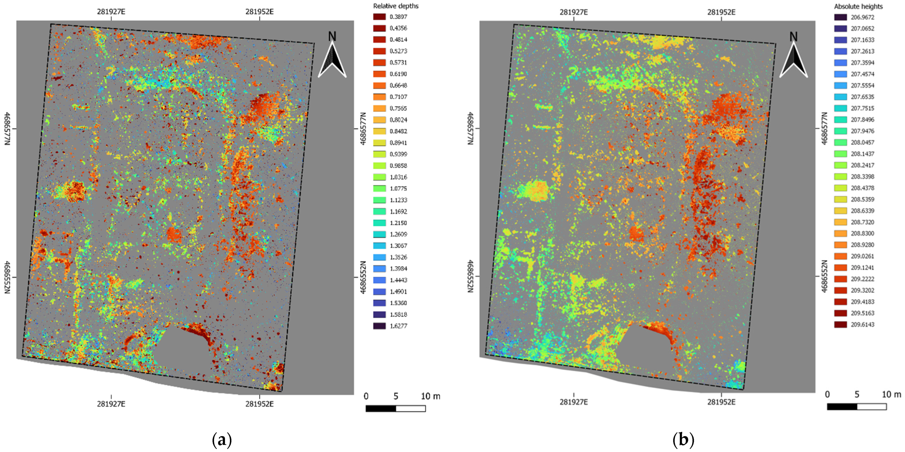
Figure 9.
Hypothetical plan of the “Capitolium” (in black) on the base of the “buried feature elevation map” (image by M. Serpetti).
Figure 9.
Hypothetical plan of the “Capitolium” (in black) on the base of the “buried feature elevation map” (image by M. Serpetti).

Figure 10.
Results of plug-in application in the bath complex area: (a) “merged signal peaks map” with estimated depth value, (b) “buried feature elevation map”, in absolute height (image by M. Serpetti).
Figure 10.
Results of plug-in application in the bath complex area: (a) “merged signal peaks map” with estimated depth value, (b) “buried feature elevation map”, in absolute height (image by M. Serpetti).
Publisher’s Note: MDPI stays neutral with regard to jurisdictional claims in published maps and institutional affiliations. |
© 2022 by the authors. Licensee MDPI, Basel, Switzerland. This article is an open access article distributed under the terms and conditions of the Creative Commons Attribution (CC BY) license (https://creativecommons.org/licenses/by/4.0/).
Share and Cite
MDPI and ACS Style
De Angeli, S.; Serpetti, M.; Battistin, F. A Newly Developed Tool for the Post-Processing of GPR Time-Slices in A GIS Environment. Remote Sens. 2022, 14, 3459. https://doi.org/10.3390/rs14143459
AMA Style
De Angeli S, Serpetti M, Battistin F. A Newly Developed Tool for the Post-Processing of GPR Time-Slices in A GIS Environment. Remote Sensing. 2022; 14(14):3459. https://doi.org/10.3390/rs14143459
Chicago/Turabian StyleDe Angeli, Stefano, Matteo Serpetti, and Fabiana Battistin. 2022. "A Newly Developed Tool for the Post-Processing of GPR Time-Slices in A GIS Environment" Remote Sensing 14, no. 14: 3459. https://doi.org/10.3390/rs14143459
Note that from the first issue of 2016, this journal uses article numbers instead of page numbers. See further details here.