
Pushbroom Photogrammetric Heights Enhance State-Level Forest Attribute Mapping with Landsat and Environmental Gradients


Abstract
:1. Introduction
2. Methods
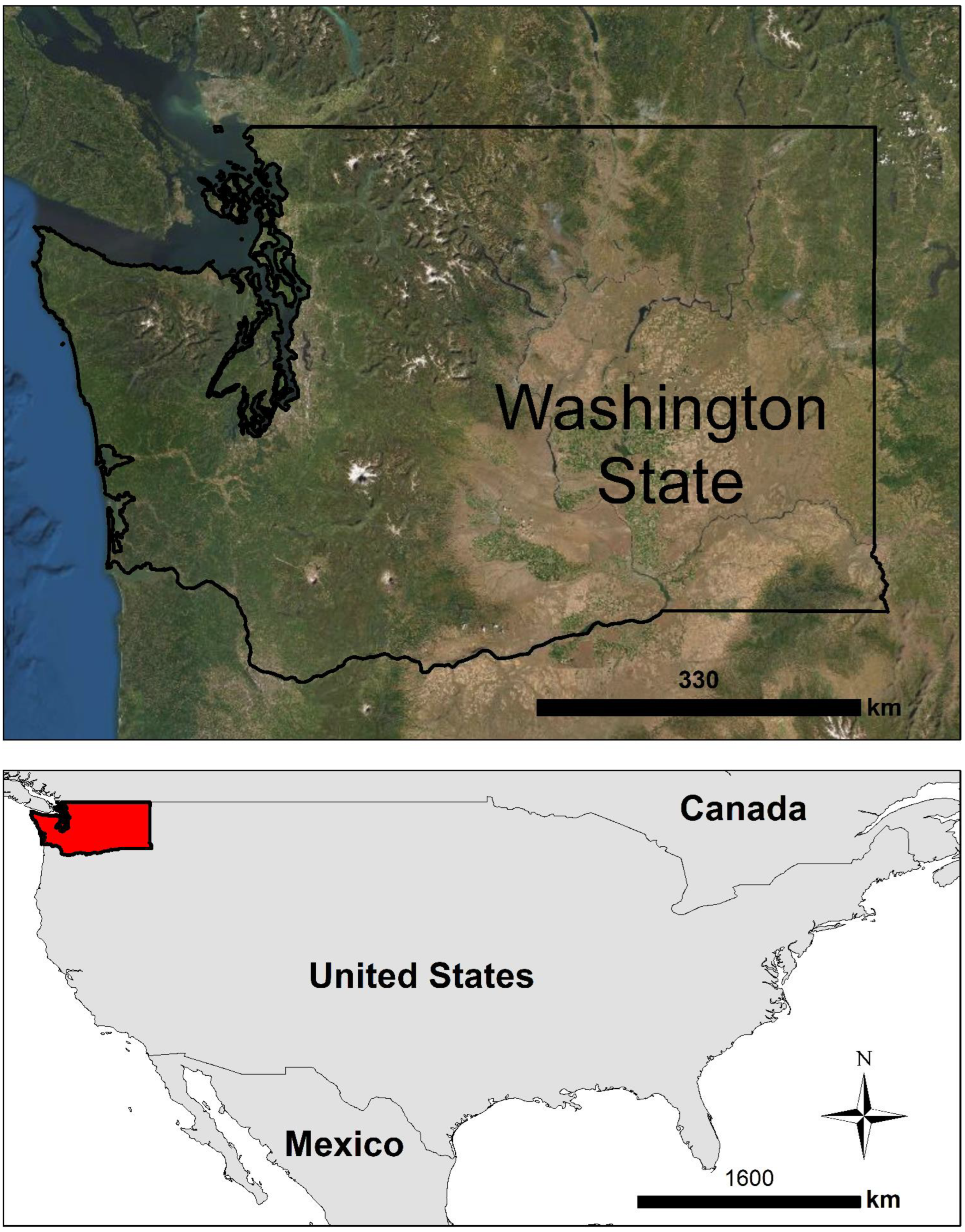
2.1. Study Area
2.2. Field Sample Data
2.3. Auxiliary Data Sources
2.4. Orthogonal Transformations
2.5. Model Exploration
3. Results
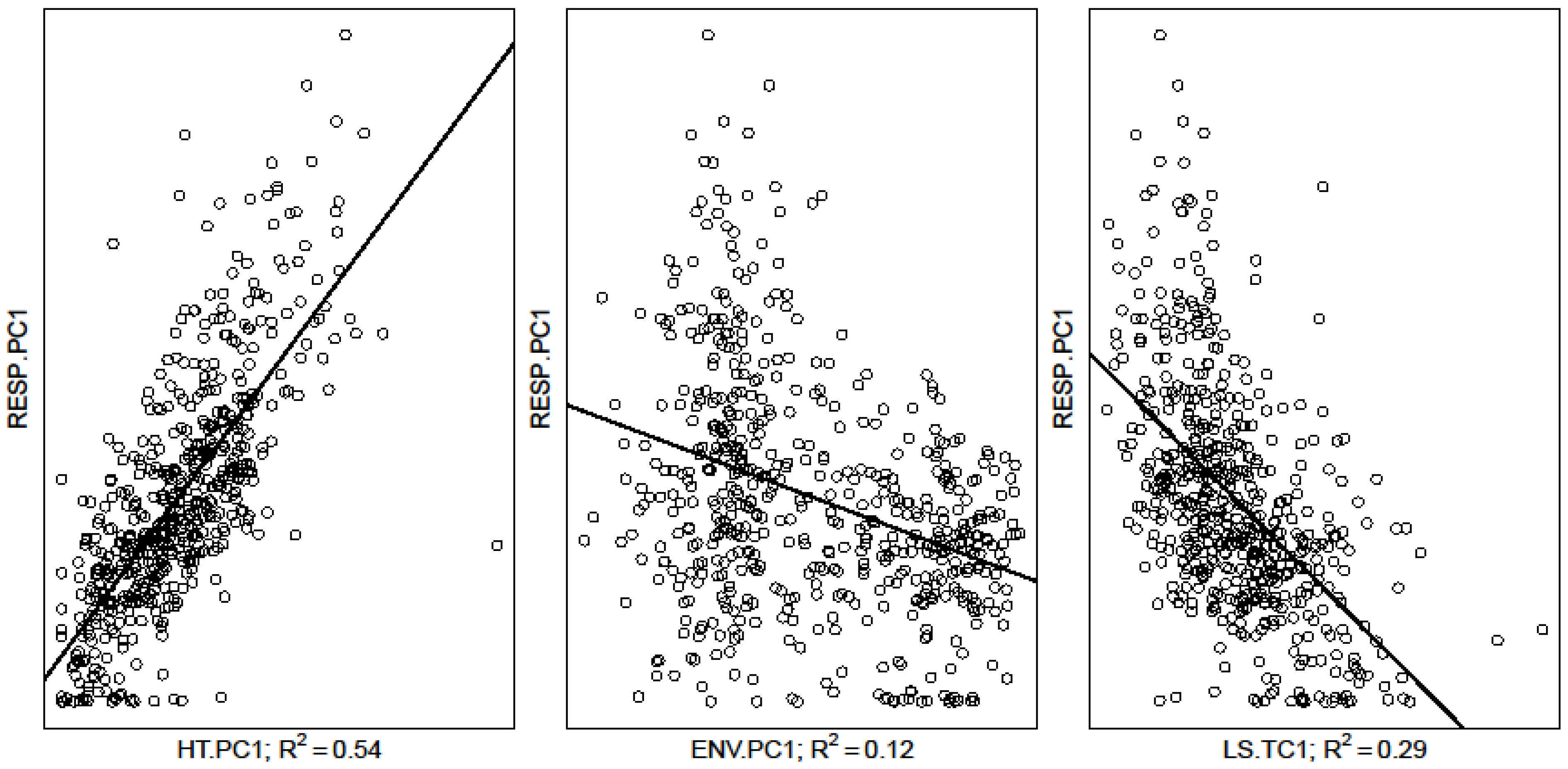
3.1. Linear Agreement between Variable Types
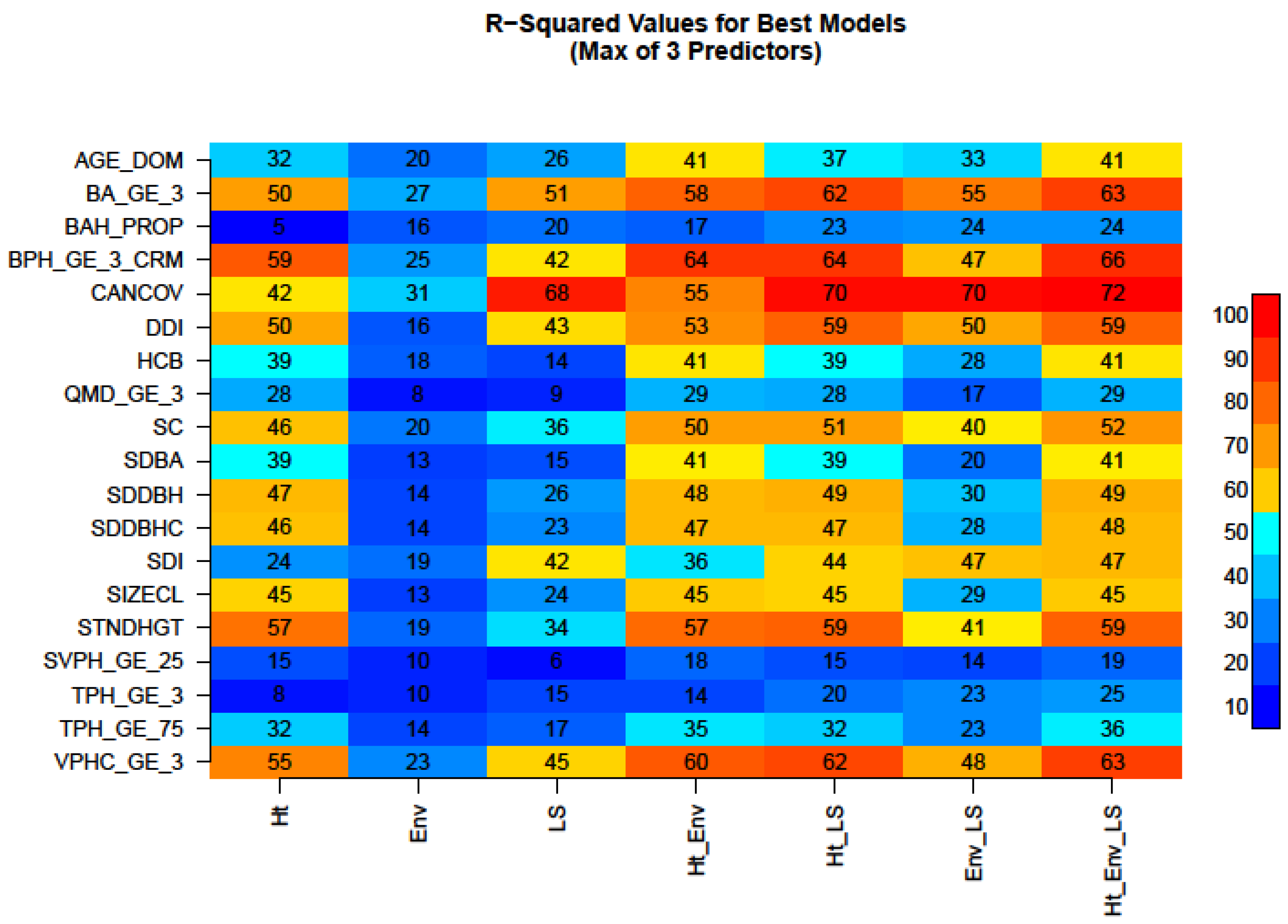
3.2. Linear Modeling Performance
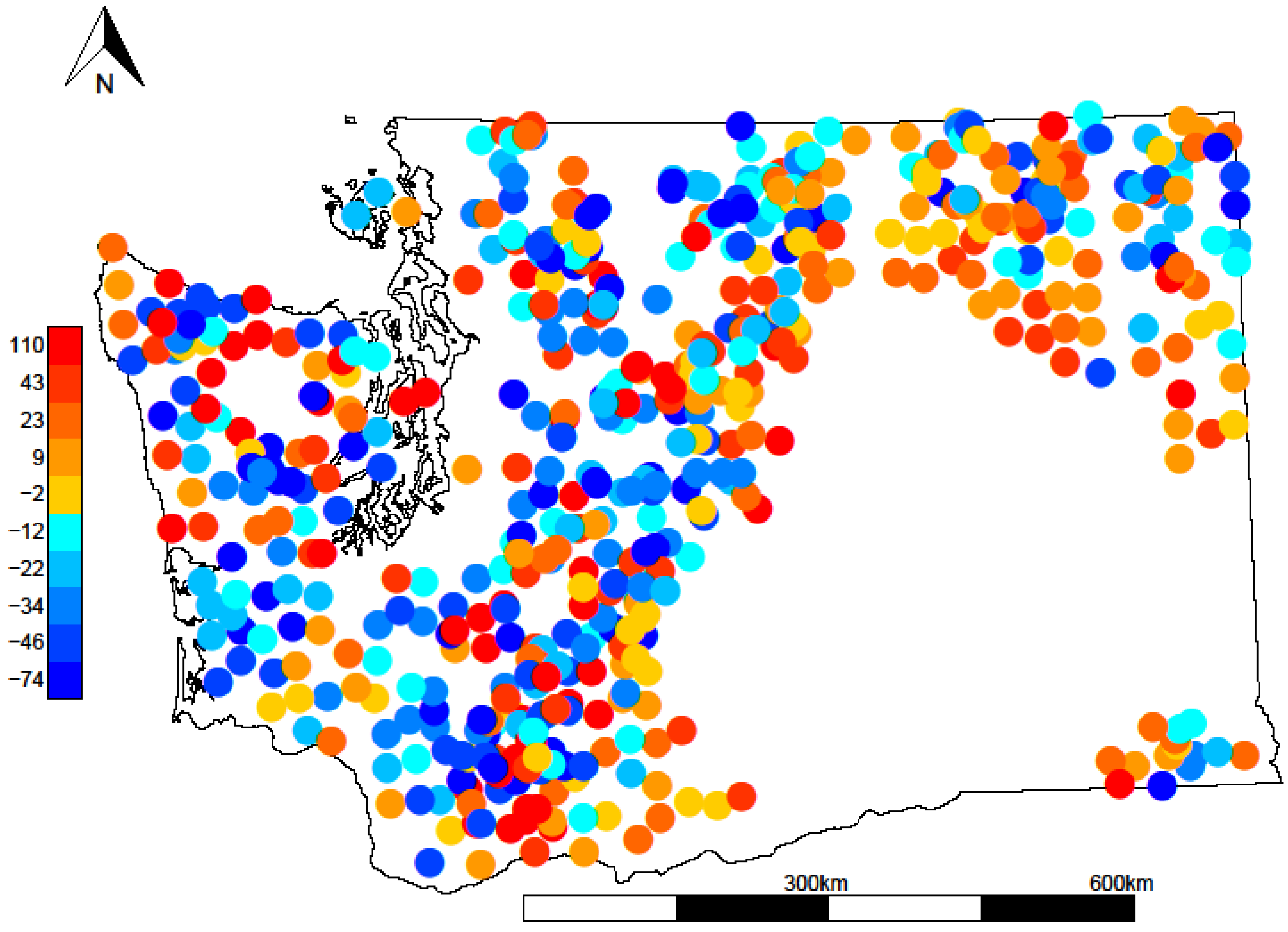
3.3. Spatial Analysis
4. Discussion
5. Conclusions
Author Contributions
Funding
Acknowledgments
Conflicts of Interest
References
- Ohmann, J.L.; Gregory, M.J. Predictive Mapping of Forest Composition and Structure with Direct Gradient Analysis and Nearest- Neighbor Imputation in Coastal Oregon, U.S.A. Can. J. For. Res. 2002, 32, 725–741. [Google Scholar] [CrossRef]
- Tomppo, E.; Olsson, H.; Ståhl, G.; Nilsson, M.; Hagner, O.; Katila, M. Combining National Forest Inventory Field Plots and Remote Sensing Data for Forest Databases. Remote Sens. Environ. 2008, 112, 1982–1999. [Google Scholar] [CrossRef]
- Wilson, B.T.; Lister, A.J.; Riemann, R.I. A Nearest-Neighbor Imputation Approach to Mapping Tree Species over Large Areas Using Forest Inventory Plots and Moderate Resolution Raster Data. For. Ecol. Manag. 2012, 271, 182–198. [Google Scholar] [CrossRef]
- White, J.C.; Coops, N.C.; Wulder, M.A.; Vastaranta, M.; Hilker, T.; Tompalski, P. Remote Sensing Technologies for Enhancing Forest Inventories: A Review. Can. J. Remote Sens. 2016, 42, 619–641. [Google Scholar] [CrossRef] [Green Version]
- Lister, A.J.; Andersen, H.; Frescino, T.; Gatziolis, D.; Healey, S.; Heath, L.S.; Liknes, G.C.; McRoberts, R.; Moisen, G.G.; Nelson, M.; et al. Use of Remote Sensing Data to Improve the Efficiency of National Forest Inventories: A Case Study from the United States National Forest Inventory. Forests 2020, 11, 1364. [Google Scholar] [CrossRef]
- Riemann, R.; Wilson, B.T.; Lister, A.; Parks, S. An Effective Assessment Protocol for Continuous Geospatial Datasets of Forest Characteristics Using USFS Forest Inventory and Analysis (FIA) Data. Remote Sens. Environ. 2010, 114, 2337–2352. [Google Scholar] [CrossRef]
- Huang, W.; Swatantran, A.; Johnson, K.; Duncanson, L.; Tang, H.; Dunne, J.O.; Hurtt, G.; Dubayah, R. Local Discrepancies in Continental Scale Biomass Maps: A Case Study over Forested and Non-Forested Landscapes in Maryland, USA. Carbon Balance Manag. 2015, 10, 19. [Google Scholar] [CrossRef] [Green Version]
- Zald, H.S.J.; Ohmann, J.L.; Roberts, H.M.; Gregory, M.J.; Henderson, E.B.; McGaughey, R.J.; Braaten, J. Influence of Lidar, Landsat Imagery, Disturbance History, Plot Location Accuracy, and Plot Size on Accuracy of Imputation Maps of Forest Composition and Structure. Remote Sens. Environ. 2014, 143, 26–38. [Google Scholar] [CrossRef]
- Steininger, M.K. Satellite Estimation of Tropical Secondary Forest Above-Ground Biomass: Data from Brazil and Bolivia. Int. J. Remote Sens. 2000, 21, 1139–1157. [Google Scholar] [CrossRef]
- Zhao, P.; Lu, D.; Wang, G.; Wu, C.; Huang, Y.; Yu, S. Examining Spectral Reflectance Saturation in Landsat Imagery and Corresponding Solutions to Improve Forest Aboveground Biomass Estimation. Remote Sens. 2016, 8, 469. [Google Scholar] [CrossRef] [Green Version]
- Sheridan, R.D.; Popescu, S.C.; Gatziolis, D.; Morgan, C.L.S.; Ku, N.-W. Modeling Forest Aboveground Biomass and Volume Using Airborne LiDAR Metrics and Forest Inventory and Analysis Data in the Pacific Northwest. Remote Sens. 2015, 7, 229–255. [Google Scholar] [CrossRef]
- Strunk, J.L.; Gould, P.J.; Packalen, P.; Gatziolis, D.; Greblowska, D.; Maki, C.; McGaughey, R.J. Evaluation of Pushbroom DAP Relative to Frame Camera DAP and Lidar for Forest Modeling. Remote Sens. Environ. 2020, 237, 111535. [Google Scholar] [CrossRef]
- Strunk, J.; Packalen, P.; Gould, P.; Gatziolis, D.; Maki, C.; Andersen, H.-E.; McGaughey, R.J. Large Area Forest Yield Estimation with Pushbroom Digital Aerial Photogrammetry. Forests 2019, 10, 397. [Google Scholar] [CrossRef] [Green Version]
- Hudak, A.T.; Lefsky, M.A.; Cohen, W.B.; Berterretche, M. Integration of Lidar and Landsat ETM+ Data for Estimating and Mapping Forest Canopy Height. Remote Sens. Environ. 2002, 82, 397–416. [Google Scholar] [CrossRef] [Green Version]
- Andersen, H.E.; Barrett, T.; Winterberger, K.; Strunk, J.; Temesgen, H. Estimating Forest Biomass on the Western Lowlands of the Kenai Peninsula of Alaska Using Airborne Lidar and Field Plot Data in a Model-Assisted Sampling Design. Proc. IUFRO Div. 2009, 4, 19–22. [Google Scholar]
- Ahmed, O.S.; Franklin, S.E.; Wulder, M.A. Integration of Lidar and Landsat Data to Estimate Forest Canopy Cover in Coastal British Columbia. Photogramm. Eng. Remote Sens. 2014, 80, 953–961. [Google Scholar] [CrossRef] [Green Version]
- Erdody, T.L.; Moskal, L.M. Fusion of LiDAR and Imagery for Estimating Forest Canopy Fuels. Remote Sens. Environ. 2010, 114, 725–737. [Google Scholar] [CrossRef]
- Singh, K.K.; Vogler, J.B.; Shoemaker, D.A.; Meentemeyer, R.K. LiDAR-Landsat Data Fusion for Large-Area Assessment of Urban Land Cover: Balancing Spatial Resolution, Data Volume and Mapping Accuracy. ISPRS J. Photogramm. Remote Sens. 2012, 74, 110–121. [Google Scholar] [CrossRef]
- Goodbody, T.R.H.; Coops, N.C.; White, J.C. Digital Aerial Photogrammetry for Updating Area-Based Forest Inventories: A Review of Opportunities, Challenges, and Future Directions. Curr. For. Rep. 2019, 5, 55–75. [Google Scholar] [CrossRef] [Green Version]
- Holgerson, J.; Stanton, S.; Waddell, K.; Palmer, M.; Kuegler, O.; Christensen, G. Washington’s Forest Resources: Forest Inventory and Analysis, 2002–2011; Gen. Tech. Rep. PNW-GTR-962; US Department of Agriculture, Forest Service, Pacific Northwest Research Station: Portland, OR, USA, 2018; p. 112. [CrossRef]
- Bechtold, W.A.; Patterson, P.L. (Eds.) The Enhanced Forest Inventory and Analysis Program: National Sampling Design and Estimation Procedures; US Department of Agriculture Forest Service, Southern Research Station: Asheville, NC, USA, 2005.
- Heath, L.S.; Hansen, M.; Smith, J.E.; Miles, P.D. Investigation into Calculating Tree Biomass and Carbon in the FIADB Using a Biomass Expansion Factor Approach. In Proceedings of the Forest Inventory and Analysis (FIA) Symposium 2008; US Department of Agriculture, Forest Service, Rocky Mountain Research Station: Park City, UT, USA, 2009; Volume 56, p. 26. [Google Scholar]
- Hann, D.W. Equations for Predicting the Largest Crown Width of Stand-Grown Trees in Western Oregon; Oregon State University: Corvallis, OR, USA, 1997. [Google Scholar]
- Franklin, J.F.; Spies, T.A.; Van Pelt, R. Definition and Inventory of Old Growth Forests on DNR-Managed State Lands (Section One). Report to the Washington Department of Natural Resources: Olympia, WA, USA, 2005; p. 22. [Google Scholar]
- Andersen, H.-E.; Strunk, J.L.; McGaughey, R.J. Using High-Performance Global Navigation Satellite System Technology to Improve Forest Inventory and Analysis Plot Coordinates in the Pacific Region. Gen. Tech. Rep. 2022, 1000, 444. [Google Scholar]
- McGaughey, R.J.; Ahmed, K.; Andersen, H.-E.; Reutebuch, S.E. Effect of Occupation Time on the Horizontal Accuracy of a Mapping-Grade GNSS Receiver under Dense Forest Canopy. Photogramm. Eng. Remote Sens. 2017, 83, 861–868. [Google Scholar] [CrossRef]
- Andersen, H.-E.; Clarkin, T.; Winterberger, K.; Strunk, J.L. An Accuracy Assessment of Positions Obtained Using Survey-and Recreational-Grade Global Positioning System Receivers across a Range of Forest Conditions within the Tanana Valley of Interior Alaska. West. J. Appl. For. 2009, 24, 128–136. [Google Scholar] [CrossRef] [Green Version]
- Clarkin, T. Modeling Global Navigation Satellite System Positional Error under Forest Canopy Based on LIDAR-Derived Canopy Densities. Master’s Thesis, University of Washington, Seattle, WA, USA, 2007. [Google Scholar]
- Daly, C.; Halbleib, M.; Smith, J.I.; Gibson, W.P.; Doggett, M.K.; Taylor, G.H.; Curtis, J.; Pasteris, P.P. Physiographically Sensitive Mapping of Climatological Temperature and Precipitation across the Conterminous United States. Int. J. Climatol. J. R. Meteorol. Soc. 2008, 28, 2031–2064. [Google Scholar] [CrossRef]
- Miller, D.A.; White, R.A. A Conterminous United States Multilayer Soil Characteristics Dataset for Regional Climate and Hydrology Modeling. Earth Interact. 1998, 2, 1–26. [Google Scholar] [CrossRef]
- McCombs, J.W.I. Geographic Information System Topographic Factor Maps for Wildlife Management. Ph.D. Thesis, Virginia Tech, Blacksburg, VA, USA, 1997. [Google Scholar]
- Pierce, K.B.; Lookingbill, T.; Urban, D. A Simple Method for Estimating Potential Relative Radiation (PRR) for Landscape-Scale Vegetation Analysis. Landsc. Ecol. 2005, 20, 137–147. [Google Scholar] [CrossRef]
- Weiss, A. Topographic position and landforms analysis. In Proceedings of the Poster Presentation, ESRI User Conference, San Diego, CA, USA, 9–13 July 2001; Volume 200. [Google Scholar]
- National Elevation Dataset (NED)|The Long Term Archive. Available online: https://lta.cr.usgs.gov/NED (accessed on 7 August 2018).
- Kennedy, R.E.; Yang, Z.; Cohen, W.B. Detecting Trends in Forest Disturbance and Recovery Using Yearly Landsat Time Series: 1. LandTrendr — Temporal Segmentation Algorithms. Remote Sens. Environ. 2010, 114, 2897–2910. [Google Scholar] [CrossRef]
- Cohen, W.B.; Yang, Z.; Healey, S.P.; Kennedy, R.E.; Gorelick, N. A LandTrendr Multispectral Ensemble for Forest Disturbance Detection. Remote Sens. Environ. 2018, 205, 131–140. [Google Scholar] [CrossRef]
- Bell, D.M.; Acker, S.A.; Gregory, M.J.; Davis, R.J.; Garcia, B.A. Quantifying Regional Trends in Large Live Tree and Snag Availability in Support of Forest Management. For. Ecol. Manag. 2021, 479, 118554. [Google Scholar] [CrossRef]
- Breiman, L. Random Forests. Mach. Learn. 2001, 45, 5–32. [Google Scholar] [CrossRef] [Green Version]
- Cohen, W.B.; Yang, Z.; Kennedy, R. Detecting Trends in Forest Disturbance and Recovery Using Yearly Landsat Time Series: 2. TimeSync–Tools for Calibration and Validation. Remote Sens. Environ. 2010, 114, 2911–2924. [Google Scholar] [CrossRef]
- Crist, E.P.; Cicone, R.C. A Physically-Based Transformation of Thematic Mapper Data—The TM Tasseled Cap. IEEE Trans. Geosci. Remote Sens. 1984, 3, 256–263. [Google Scholar] [CrossRef]
- Lutes, D.C.; Keane, R.E.; Caratti, J.F.; Key, C.H.; Benson, N.C.; Sutherland, S.; Gangi, L.J. FIREMON: Fire Effects Monitoring and Inventory System; US Department of Agriculture, Forest Service, Rocky Mountain Research Station: Fort Collins, CO, USA, 2006; p. 164.
- Walker, S.; Pietrzak, A. Remote Measurement Methods for 3-D Modeling Purposes Using BAE Systems’ Software. Geod. Cartogr. 2015, 64, 113–124. [Google Scholar] [CrossRef]
- Isenburg, M. LASzip: Lossless Compression of LiDAR Data. Photogramm. Eng. Remote Sens. 2013, 79, 209–217. [Google Scholar] [CrossRef]
- Gesch, D.B.; Evans, G.A.; Oimoen, M.J.; Arundel, S. The National Elevation Dataset. 2018; pp. 83–110. Available online: https://pubs.er.usgs.gov/publication/70201572 (accessed on 7 August 2018).
- McGaughey, R.J. FUSION/LDV: Software for LiDAR Data Analysis and Visualization [Computer Program]; USDA, Forest Service Pacific Northwest Research Station: Washington, DC, USA, 2014.
- Kauth, R.J.; Thomas, G.S. The Tasselled Cap—A Graphic Description of the Spectral-Temporal Development of Agricultural Crops as Seen by Landsat. In Proceedings of the LARS Symposia; Purdue University: West Lafayette, Indiana, 1976; p. 159. [Google Scholar]
- R Core Team. R: A Language and Environment for Statistical Computing; R Core Team: Vienna, Austria, 2020. [Google Scholar]
- RStudio Team. RStudio: Integrated Development Environment for r; RStudio Team: Boston, MA, USA, 2020. [Google Scholar]
- Furnival, G.M.; Wilson, R.W., Jr. Regressions by Leaps and Bounds. Technometrics 1974, 16, 499–511. [Google Scholar] [CrossRef]
- Schwarz, G. Estimating the Dimension of a Model. Ann. Stat. 1978, 6, 461–464. [Google Scholar] [CrossRef]
- Moran, P.A.P. Notes on Continuous Stochastic Phenomena. Biometrika 1950, 37, 17–23. [Google Scholar] [CrossRef] [PubMed]
- Riemann, R.; Liknes, G.; O’Neil-Dunne, J.; Toney, C.; Lister, T. Comparative Assessment of Methods for Estimating Tree Canopy Cover across a Rural-to-Urban Gradient in the Mid-Atlantic Region of the USA. Environ. Monit. Assess. 2016, 188, 297. [Google Scholar] [CrossRef]
- Davis, R.J.; Ohmann, J.L.; Kennedy, R.E.; Cohen, W.B.; Gregory, M.J.; Yang, Z.; Roberts, H.M.; Gray, A.N.; Spies, T.A. Northwest Forest Plan–the First 20 Years (1994-2013): Status and Trends of Late-Successional and Old-Growth Forests. Gen Tech Rep PNW-GTR-911 Portland US Dep. Agric. For. Serv. Pac. Northwest Res. Stn. 112 P 2015, 911. [Google Scholar]
- Babcock, C.; Finley, A.O.; Andersen, H.-E.; Pattison, R.; Cook, B.D.; Morton, D.C.; Alonzo, M.; Nelson, R.; Gregoire, T.; Ene, L.; et al. Geostatistical Estimation of Forest Biomass in Interior Alaska Combining Landsat-Derived Tree Cover, Sampled Airborne Lidar and Field Observations. Remote Sens. Environ. 2018, 212, 212–230. [Google Scholar] [CrossRef] [Green Version]
- Fuller, W.A. Measurement Error Models; John Wiley and Sons: Hoboken, NJ, USA, 1987; ISBN 978-0-471-86187-4. [Google Scholar]
- Hengl, T.; Heuvelink, G.B.M.; Rossiter, D.G. About Regression-Kriging: From Equations to Case Studies. Comput. Geosci. 2007, 33, 1301–1315. [Google Scholar] [CrossRef]
- Packalén, P.; Temesgen, H.; Maltamo, M. Variable Selection Strategies for Nearest Neighbor Imputation Methods Used in Remote Sensing Based Forest Inventory. Can. J. Remote Sens. 2012, 38, 557–569. [Google Scholar] [CrossRef]
- Powell, S.L.; Cohen, W.B.; Healey, S.P.; Kennedy, R.E.; Moisen, G.G.; Pierce, K.B.; Ohmann, J.L. Quantification of Live Aboveground Forest Biomass Dynamics with Landsat Time-Series and Field Inventory Data: A Comparison of Empirical Modeling Approaches. Remote Sens. Environ. 2010, 114, 1053–1068. [Google Scholar] [CrossRef]
- Bell, D.M.; Gregory, M.J.; Kane, V.; Kane, J.; Kennedy, R.E.; Roberts, H.M.; Yang, Z. Multiscale Divergence between Landsat-and Lidar-Based Biomass Mapping Is Related to Regional Variation in Canopy Cover and Composition. Carbon Balance Manag. 2018, 13, 1–14. [Google Scholar] [CrossRef] [PubMed] [Green Version]
- Kennedy, R.E.; Ohmann, J.; Gregory, M.; Roberts, H.; Yang, Z.; Bell, D.M.; Kane, V.; Hughes, M.J.; Cohen, W.B.; Powell, S. An Empirical, Integrated Forest Biomass Monitoring System. Environ. Res. Lett. 2018, 13, 025004. [Google Scholar] [CrossRef]
- Noordermeer, L.; Bollandsås, O.M.; Ørka, H.O.; Næsset, E.; Gobakken, T. Comparing the Accuracies of Forest Attributes Predicted from Airborne Laser Scanning and Digital Aerial Photogrammetry in Operational Forest Inventories. Remote Sens. Environ. 2019, 226, 26–37. [Google Scholar] [CrossRef]
- Fiala, A.C.S.; Garman, S.L.; Gray, A.N. Comparison of Five Canopy Cover Estimation Techniques in the Western Oregon Cascades. For. Ecol. Manag. 2006, 232, 188–197. [Google Scholar] [CrossRef]
- Henderson, E.B.; Ohmann, J.L.; Gregory, M.J.; Roberts, H.M.; Zald, H. Species Distribution Modelling for Plant Communities: Stacked Single Species or Multivariate Modelling Approaches? Appl. Veg. Sci. 2014, 17, 516–527. [Google Scholar] [CrossRef]


| Attribute | Units | Description |
|---|---|---|
| AGE_DOM | years | Basal area weighted stand age based on field recorded or modeled ages of open grown, dominant, and co-dominant trees (FIA crown classes 1–3) |
| BA_GE_3 | m2/ha | Basal area of live trees ≥2.5 cm DBH |
| BAH_PROP | proportion | Proportion of total basal area that is hardwood |
| BPH_GE_3_CRM | kg/ha | Component Ratio Method biomass of all live trees ≥2.5 cm DBH [22] |
| CANCOV | percent | Canopy cover of all live trees [23] |
| DDI | none | Diameter diversity index [24] |
| HCB | m | Average height to crown base |
| QMD_GE_3 | cm | Quadratic mean diameter of trees ≥2.5 cm DBH |
| SC | none | A composite measure of stand size class and stand cover class. |
| SDBA | m2/ha | Standard deviation of basal area of all live trees |
| SDDBH | cm | Standard deviation of diameter of all live trees |
| SDDBHC | cm | Standard deviation of diameter of all live conifers |
| SDI | none | Stand density index, defined as sqrt (trees per hectare × basal area per hectare) |
| SIZECL | none | Ordinal size class based on quadratic mean diameter of dominant and co-dominant trees (QMD). |
| STNDHGT | m | Average tree height of dominant and codominant trees |
| SVPH_GE_25 | m3/ha | Volume of snags ≥25.0 cm DBH and ≥ 2.0 m tall |
| TPH_GE_3 | trees/ha | Density of live trees ≥ 2.5 cm DBH |
| TPH_GE_75 | trees/ha | Density of live trees ≥ 75.0 cm DBH |
| VPHC_GE_3 | m3/ha | Volume of live conifers ≥ 2.5 cm DBH |
| Min | Max | Mean | Median | sd | cv% | |
|---|---|---|---|---|---|---|
| VPHC_GE_3 | 0 | 1747.45 | 348.87 | 232.82 | 351.82 | 100.84 |
| TPH_GE_75 | 0 | 113.57 | 8.13 | 0 | 17.37 | 213.53 |
| TPH_GE_3 | 0 | 7466.23 | 1009.72 | 700.67 | 1052.42 | 104.23 |
| SVPH_GE_25 | 0 | 1119.22 | 85.02 | 26.69 | 143.92 | 169.29 |
| STNDHGT | 0 | 64.68 | 20.12 | 19.54 | 11.5 | 57.17 |
| SIZECL | 1 | 6 | 3.23 | 3 | 1.23 | 38.13 |
| SDI | 0 | 693.67 | 169.37 | 152.06 | 120.9 | 71.38 |
| SDDBHC | 0 | 44.24 | 12.28 | 11.41 | 7.65 | 62.3 |
| SDDBH | 0 | 42.25 | 12.23 | 11.45 | 7.39 | 60.44 |
| SDBA | 0 | 0.61 | 0.07 | 0.05 | 0.08 | 103.33 |
| SC | 1 | 7 | 4.15 | 4 | 1.71 | 41.26 |
| QMD_GE_3 | 0 | 100.57 | 24.31 | 22.86 | 13.34 | 54.88 |
| HCB | 0 | 30.42 | 7.1 | 5.89 | 5.62 | 79.25 |
| DDI | 0 | 10 | 3.99 | 3.58 | 2.25 | 56.45 |
| CANCOV | 0 | 99.57 | 63.67 | 70.79 | 27.95 | 43.9 |
| BPH_GE_3_CRM | 0 | 996,580.22 | 199,977.61 | 141,155.54 | 198,912.17 | 99.47 |
| BAH_PROP | 0 | 1 | 0.05 | 0 | 0.16 | 313.39 |
| BA_GE_3 | 0 | 128.54 | 35.67 | 30.15 | 26.41 | 74.05 |
| AGE_DOM | 0 | 526 | 111.36 | 94 | 82.03 | 73.67 |
| Attribute | Units | Description |
|---|---|---|
| Climate (based on PRISM 30-year normals—1981–2010) | ||
| ANNPRE | ln mm | Total annual precipitation |
| ANNTMP | °C | Mean annual temperature |
| AUGMAXT | °C | Mean August maximum temperature |
| CONTPRE | % | Percentage of annual precipitation falling in June–August |
| CVPRE | none | Coefficient of variation of mean monthly precipitation of December and July |
| DECMINT | °C | Mean December minimum temperature |
| DIFTMP | °C | Difference between AUGMAXT and DECMINT |
| SMRMAXVPD | hPa | Maximum summer vapor pressure deficit |
| SMRMNVPD | hPa | Mean summer vapor pressure deficit |
| SMRPRE | ln mm | Mean precipitation from May–September |
| SMRTMP | °C | Mean temperature from May–September |
| Location | ||
| LAT | none | Geographic latitude |
| LON | none | Geographic longitude |
| COASTPROX | none | Coastal proximity for temperature |
| Soils | ||
| AWCL1 | none | Available water capacity up to one meter |
| ROCKDEPTH | cm | Soil rock depth |
| BD | none | Soil bulk density |
| SAND | % | Soil percent sand |
| SILT | % | Soil percent silt |
| CLAY | % | Soil percent clay |
| PERM | none | Soil permeability |
| PH | none | Soil pH |
| POROS | none | Soil porosity |
| RVOL | none | Soil rock volume |
| Topography | ||
| DEM | meters | Elevation |
| HILL | none | Elevation hillshade from azimuth = 315, altitude = 45 |
| MLI | none | McComb’s Landform Index [31] |
| SLPPCT | % | Slope (percent) (rounded to nearest integer) |
| PRR | none | Potential relative radiation [32] |
| TPI150 | none | Topographic position index, calculated as difference between cell’s elevation and mean elevation of cells within a 150-m-radius window [33] |
| TPI300 | none | Topographic position index, calculated as difference between cell’s elevation and mean elevation of cells within a 150–300-m-radius annulus |
| TPI450 | none | Topographic position index, calculated as difference between cell’s elevation and mean elevation of cells within a 300–450-m-radius annulus |
| Attribute | Units | Description |
|---|---|---|
| TC1 | none | Fitted tasseled-cap axis 1 (brightness) based on ensemble Landtrendr segmentation |
| TC2 | none | Fitted tasseled-cap axis 2 (greenness) based on ensemble Landtrendr segmentation |
| TC3 | none | Fitted tasseled-cap axis 3 (wetness) based on ensemble Landtrendr segmentation |
| NBR | none | Fitted normalized burn ratio based on ensemble Landtrendr segmentation |
| Attribute | Units | Description |
|---|---|---|
| Min, max, median, mean, sd, skewness, kurtosis | meters | Various statistics computed on vertical distribution of point heights above 2 m. Points below 2 m were not considered. |
| P05, P50, P90 | meters | Height quantiles computed on the vertical distribution of point heights above 2 m. Points below 2 m were not considered. |
| Cover | % | Percent of points above 2 m relative to all points |
Publisher’s Note: MDPI stays neutral with regard to jurisdictional claims in published maps and institutional affiliations. |
© 2022 by the authors. Licensee MDPI, Basel, Switzerland. This article is an open access article distributed under the terms and conditions of the Creative Commons Attribution (CC BY) license (https://creativecommons.org/licenses/by/4.0/).
Share and Cite
Strunk, J.L.; Bell, D.M.; Gregory, M.J. Pushbroom Photogrammetric Heights Enhance State-Level Forest Attribute Mapping with Landsat and Environmental Gradients. Remote Sens. 2022, 14, 3433. https://doi.org/10.3390/rs14143433
Strunk JL, Bell DM, Gregory MJ. Pushbroom Photogrammetric Heights Enhance State-Level Forest Attribute Mapping with Landsat and Environmental Gradients. Remote Sensing. 2022; 14(14):3433. https://doi.org/10.3390/rs14143433
Chicago/Turabian StyleStrunk, Jacob L., David M. Bell, and Matthew J. Gregory. 2022. "Pushbroom Photogrammetric Heights Enhance State-Level Forest Attribute Mapping with Landsat and Environmental Gradients" Remote Sensing 14, no. 14: 3433. https://doi.org/10.3390/rs14143433
APA StyleStrunk, J. L., Bell, D. M., & Gregory, M. J. (2022). Pushbroom Photogrammetric Heights Enhance State-Level Forest Attribute Mapping with Landsat and Environmental Gradients. Remote Sensing, 14(14), 3433. https://doi.org/10.3390/rs14143433