
Monitoring the Distribution and Variations of City Size Based on Night-Time Light Remote Sensing: A Case Study in the Yangtze River Delta of China

 , ,
, , 
Abstract
:
1. Introduction
2. Methodology
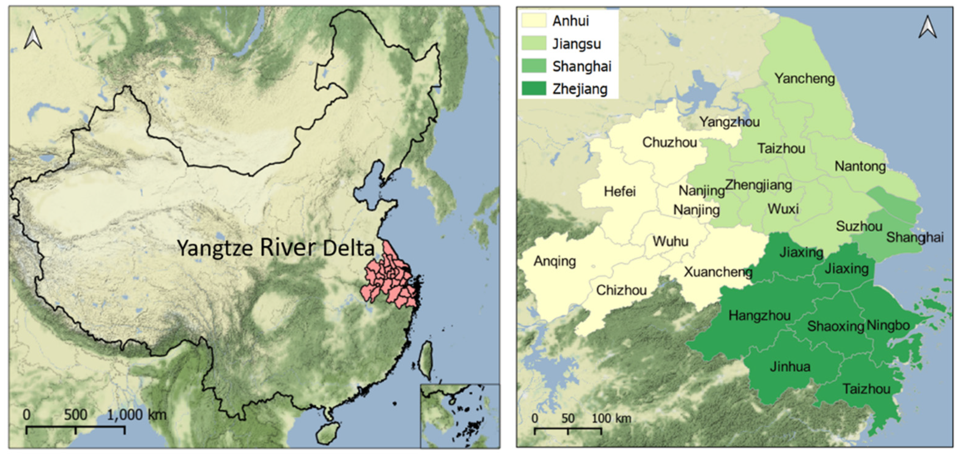
2.1. Study Area
2.2. Data Collection and Preprocessing
2.3. Monitoring of the Distribution and Variations in City Size
2.3.1. Rank–Size Rule
2.3.2. Law of Primate City
2.3.3. Gini Coefficient
2.4. Urban Area Extraction
3. Results and Discussion
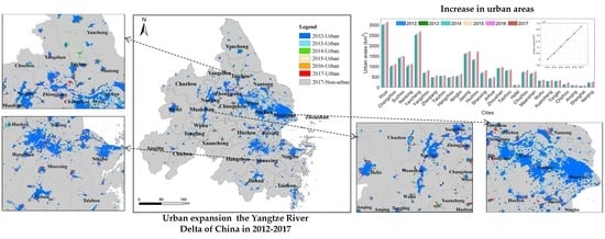
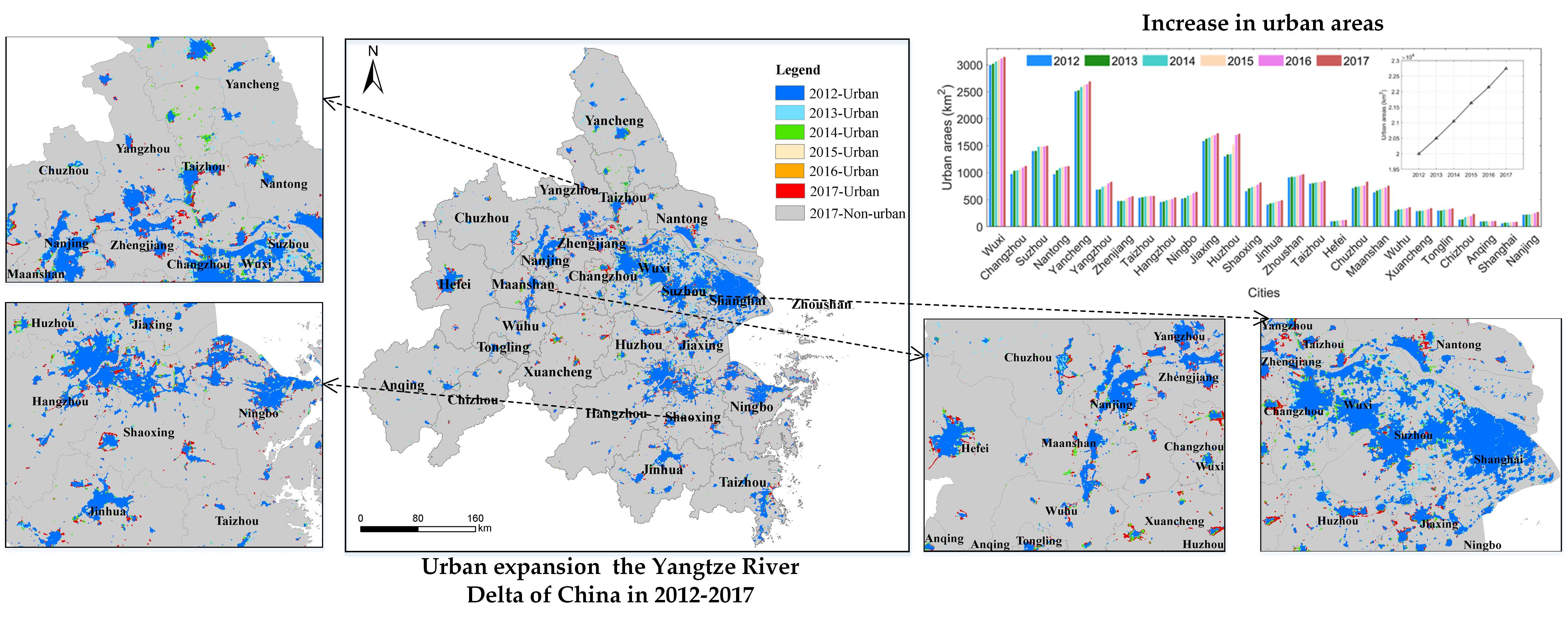
3.1. Urban Expansion of the YRD
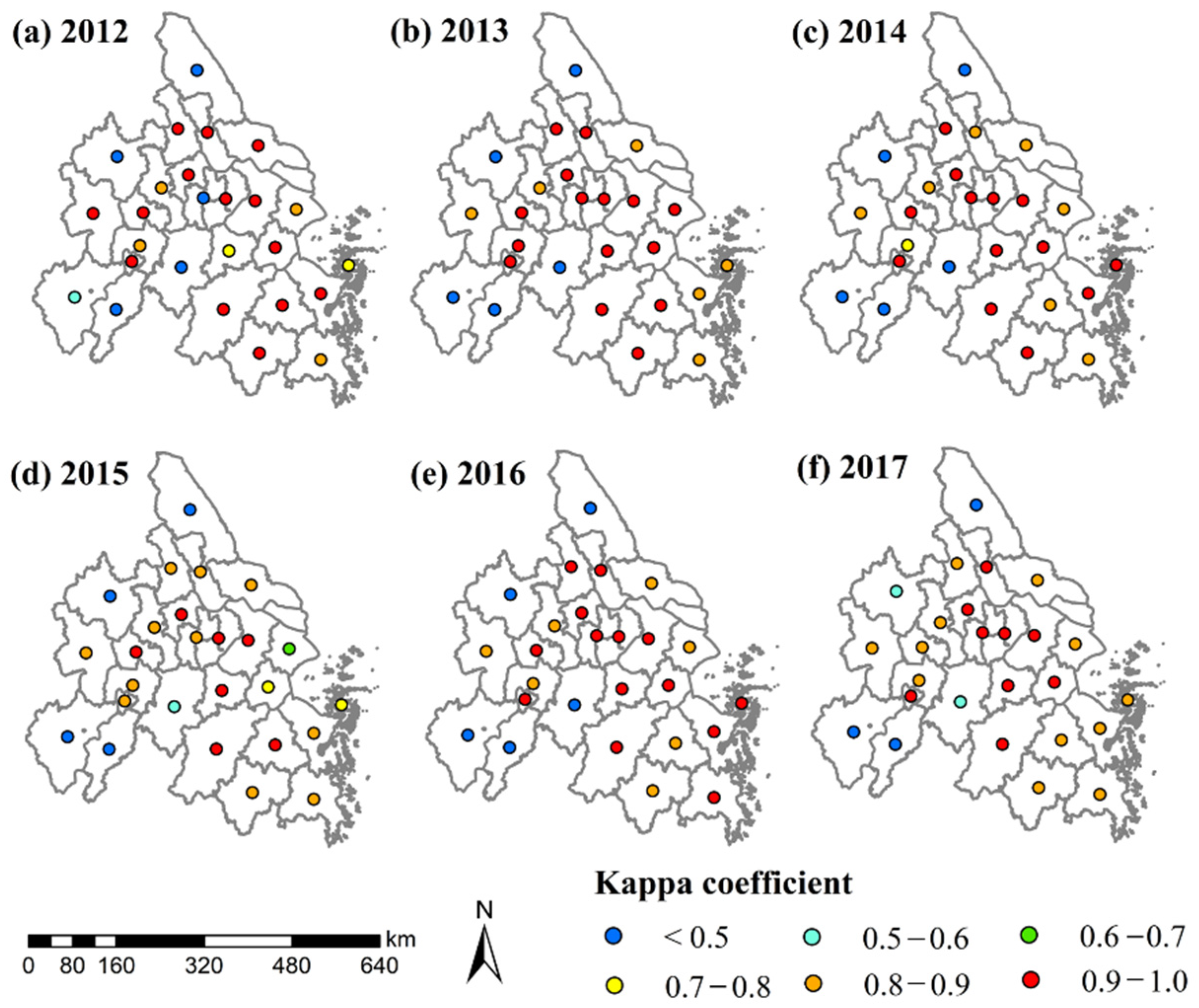
3.1.1. Accuracy Assessment of Urban Area Extraction
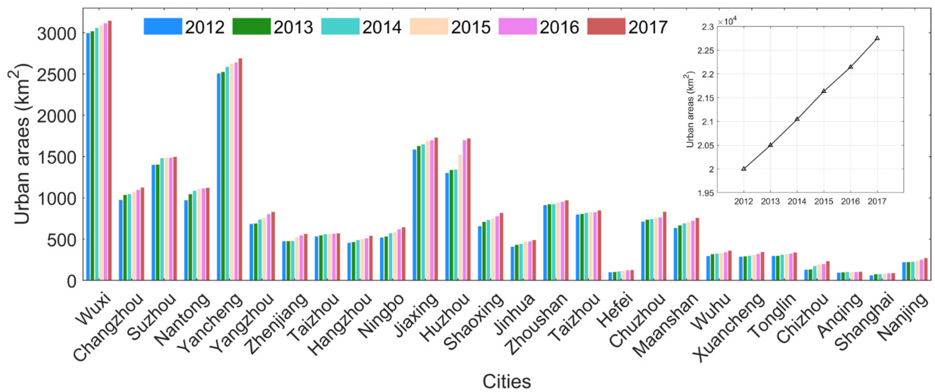
3.1.2. Spatial–Temporal Variations of Urban Areas
3.2. Variations in City Size in the YRD
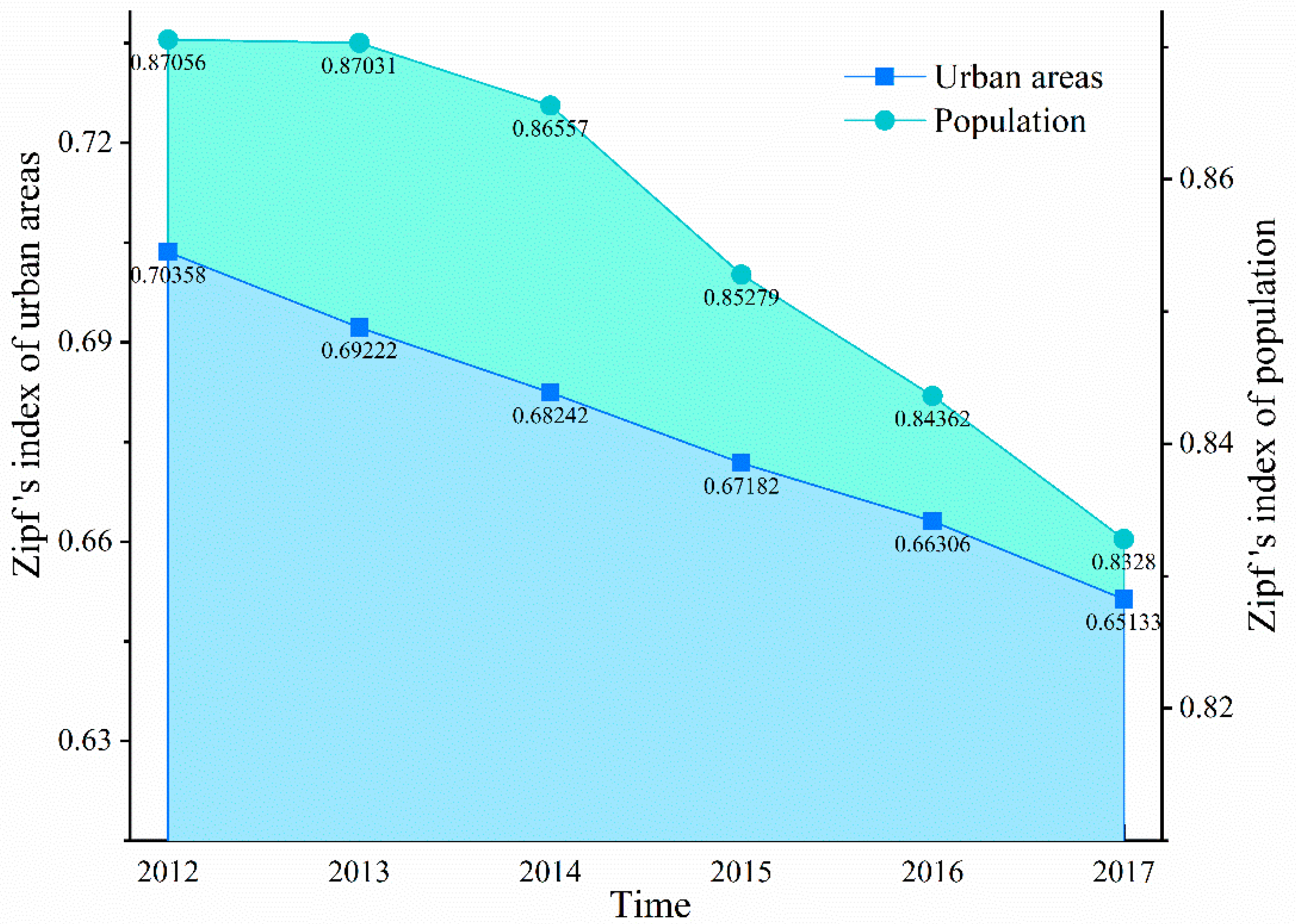
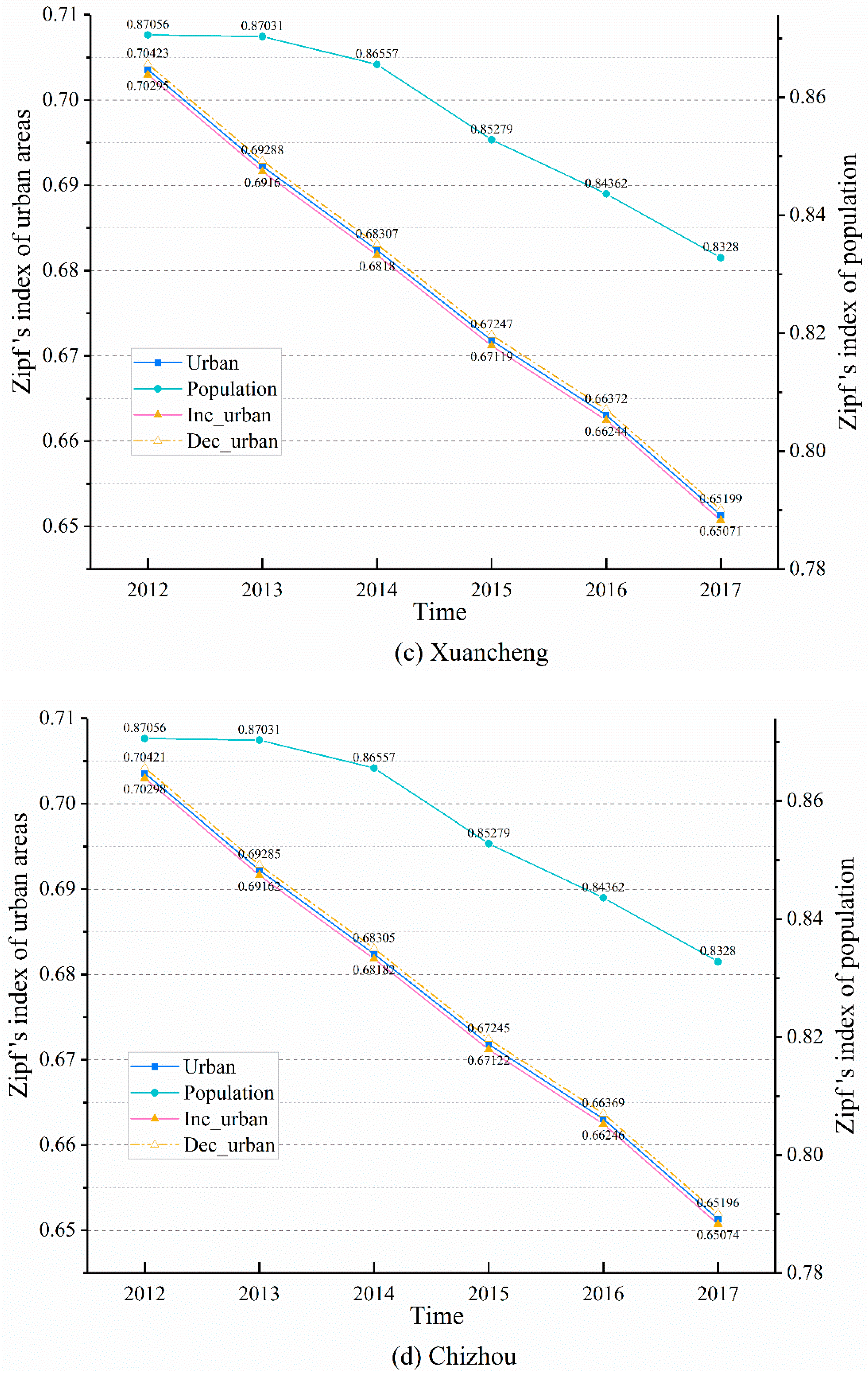
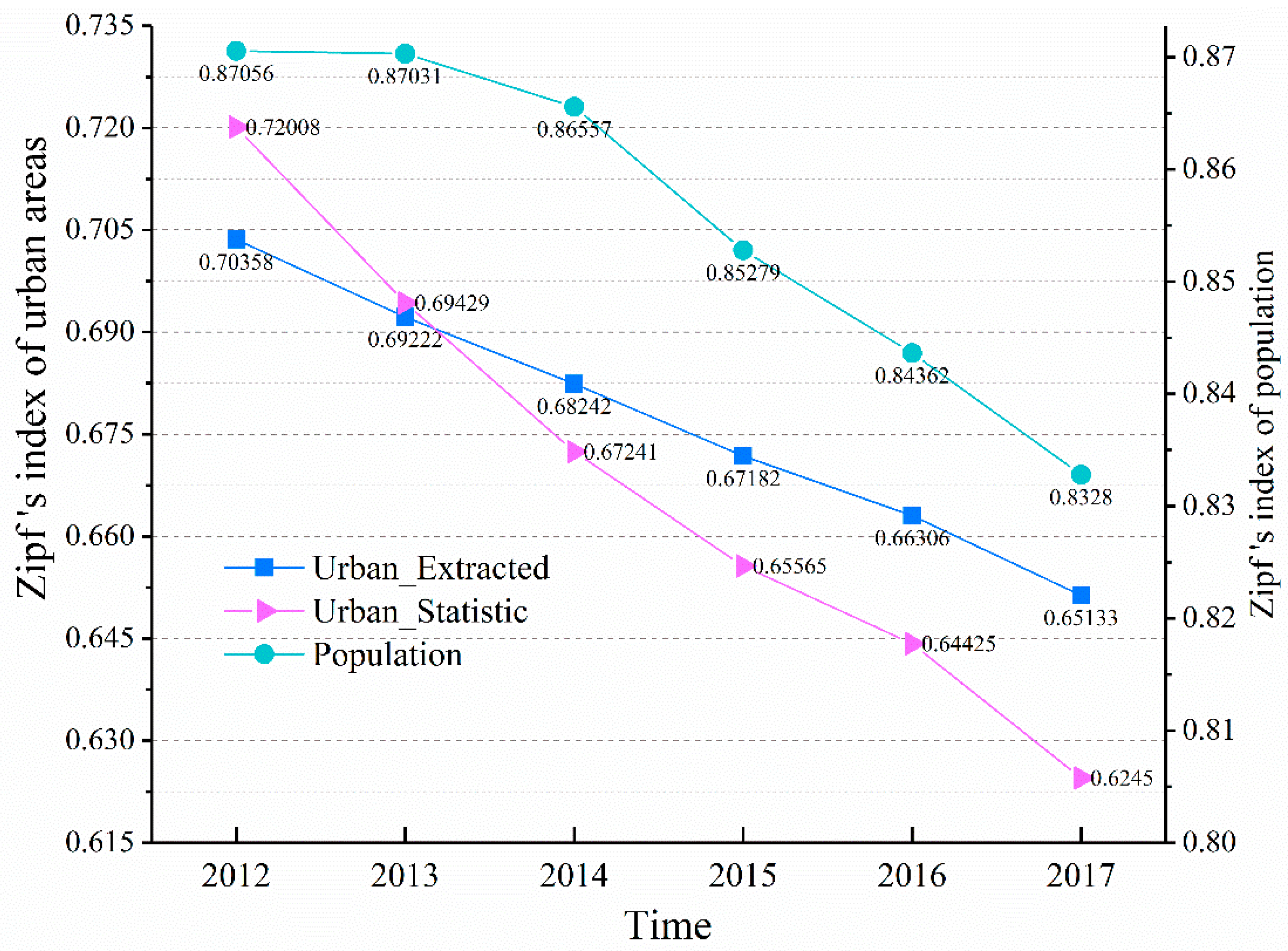
3.2.1. Variations in Rank–Size
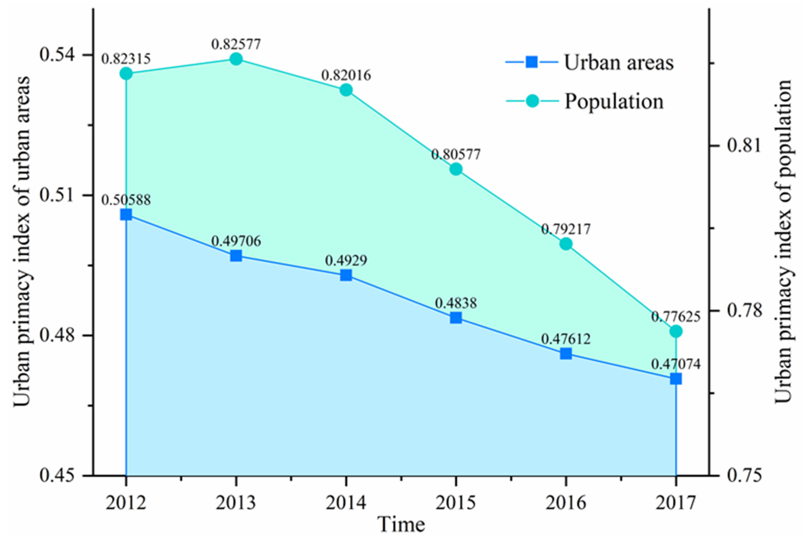
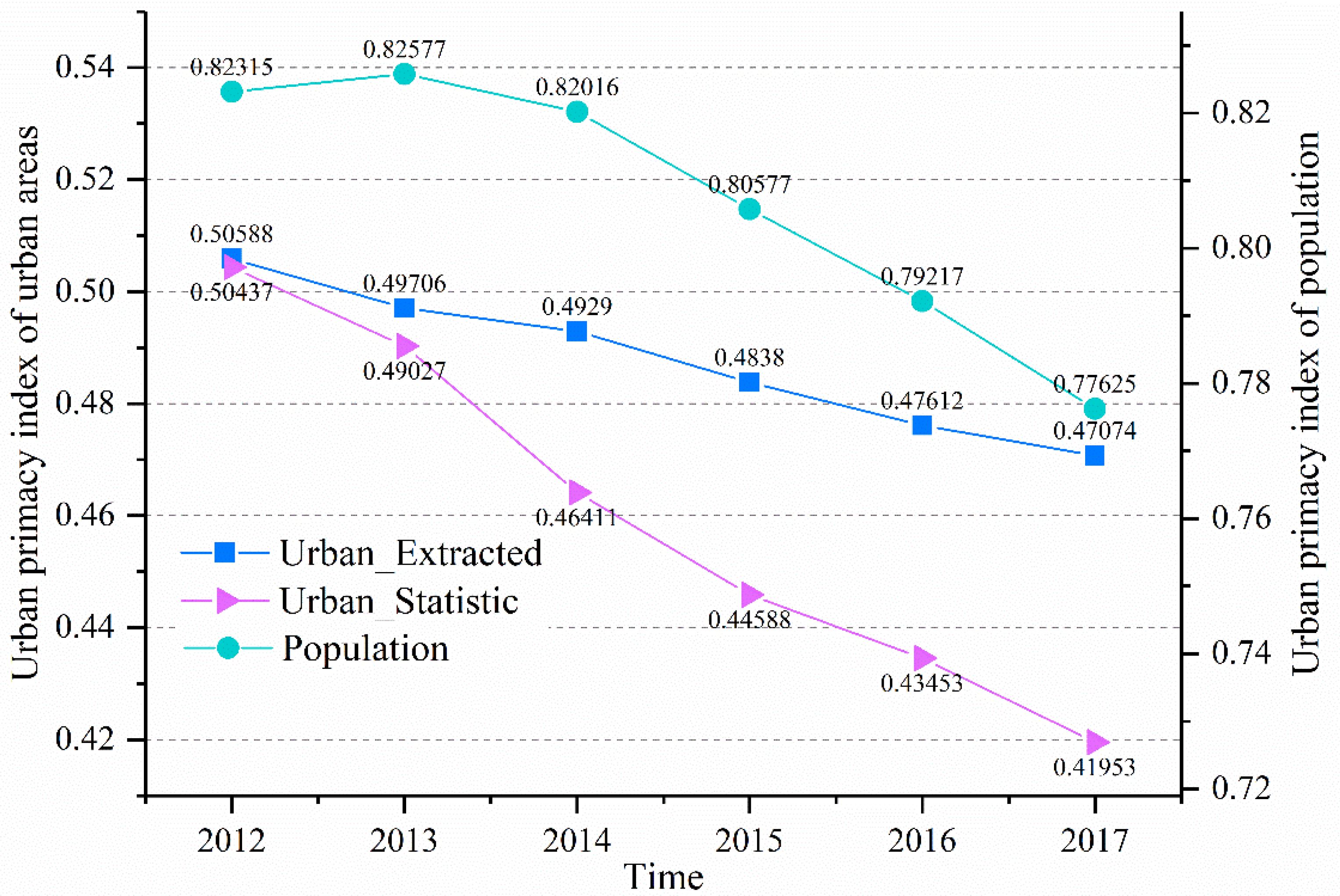
3.2.2. Variations in Primate City
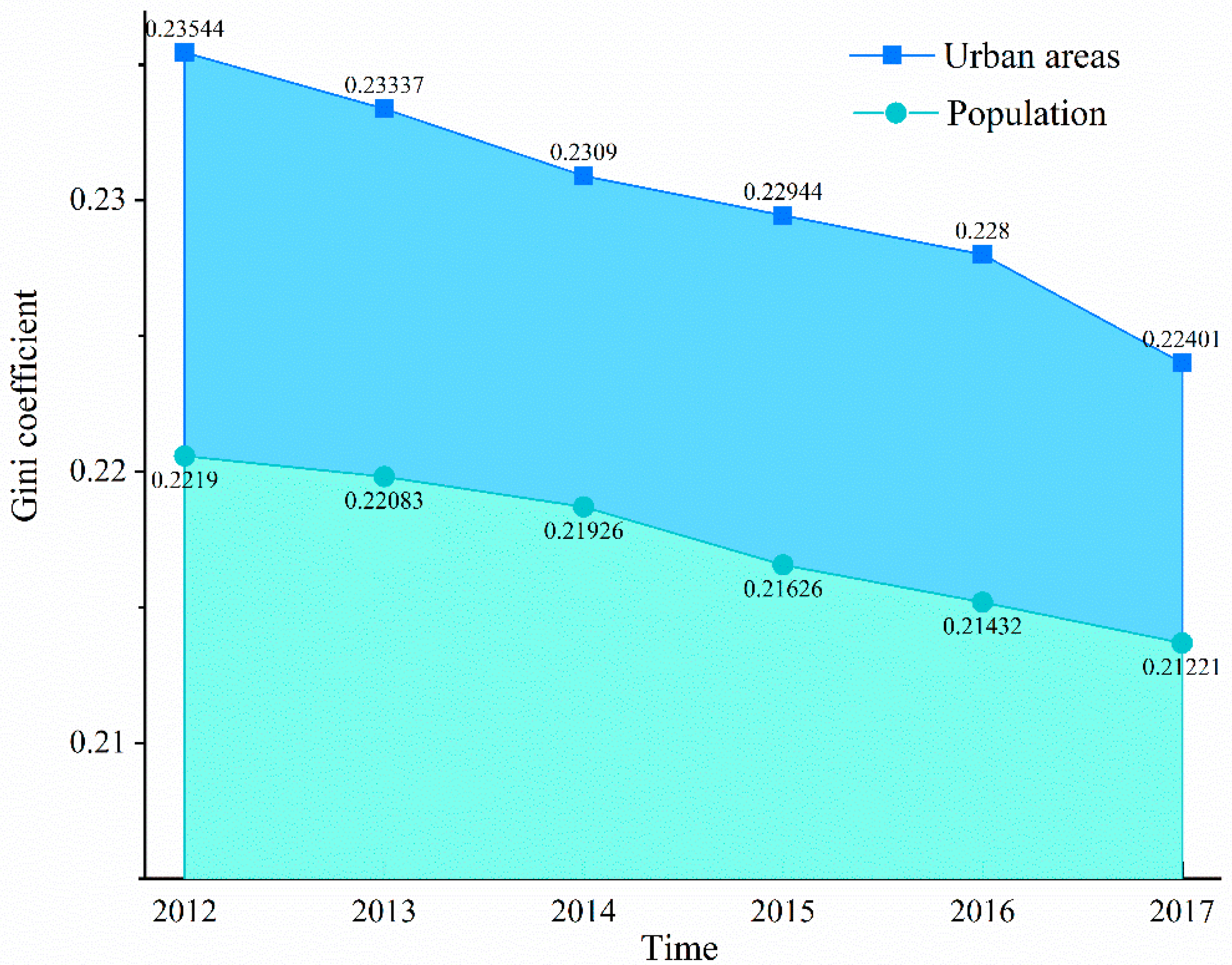
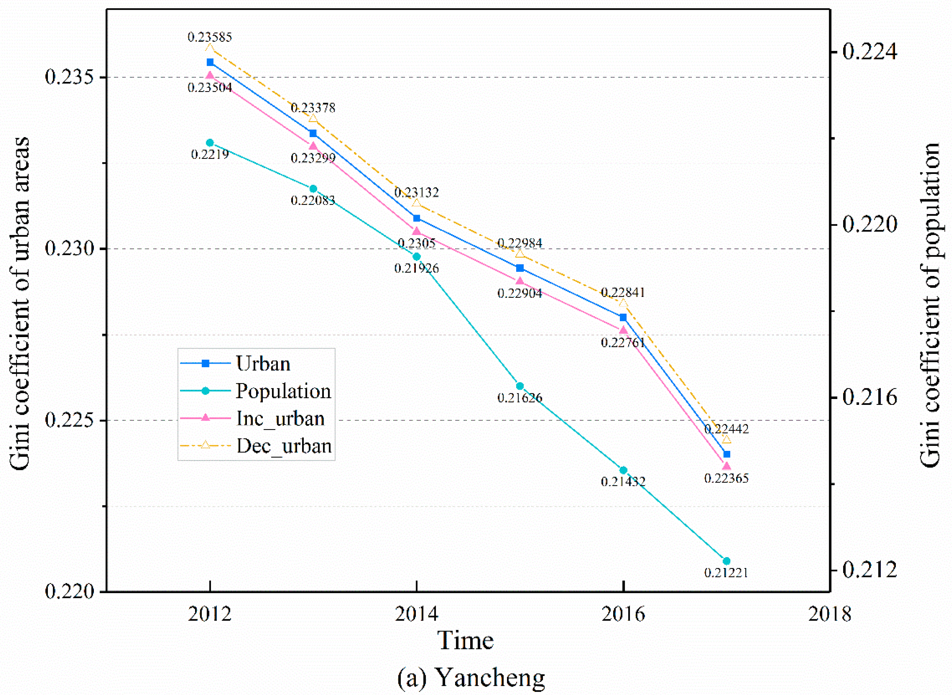
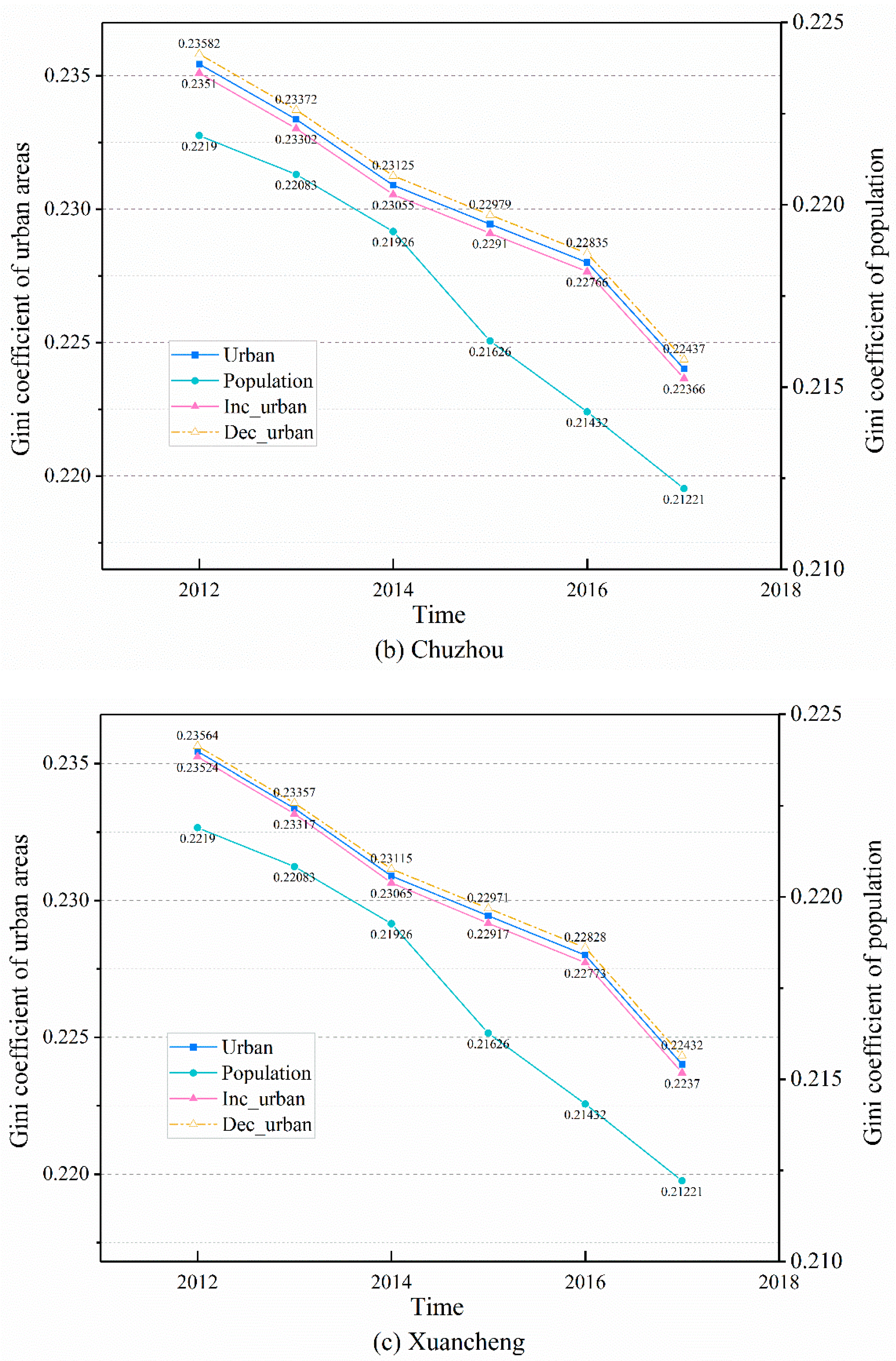
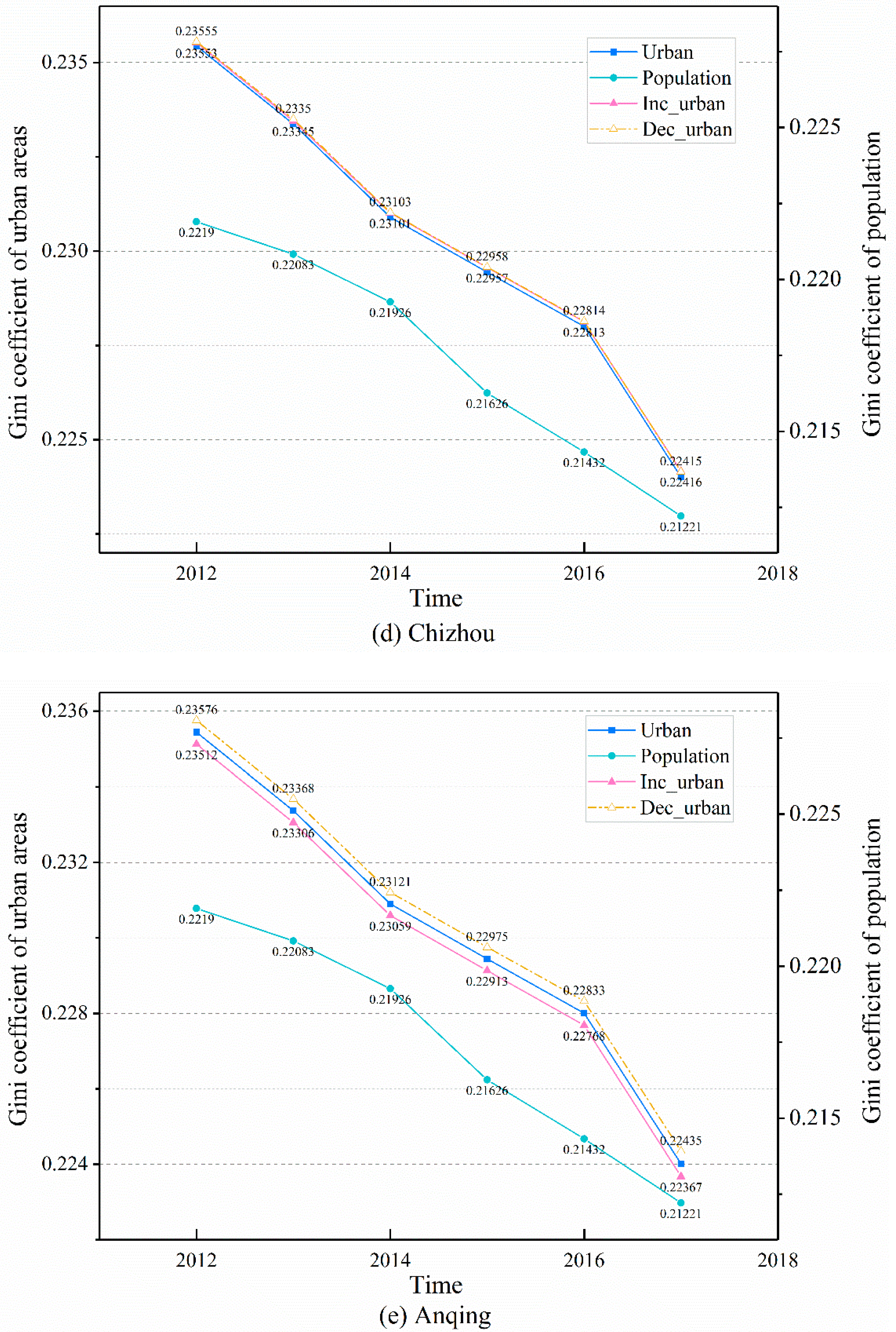
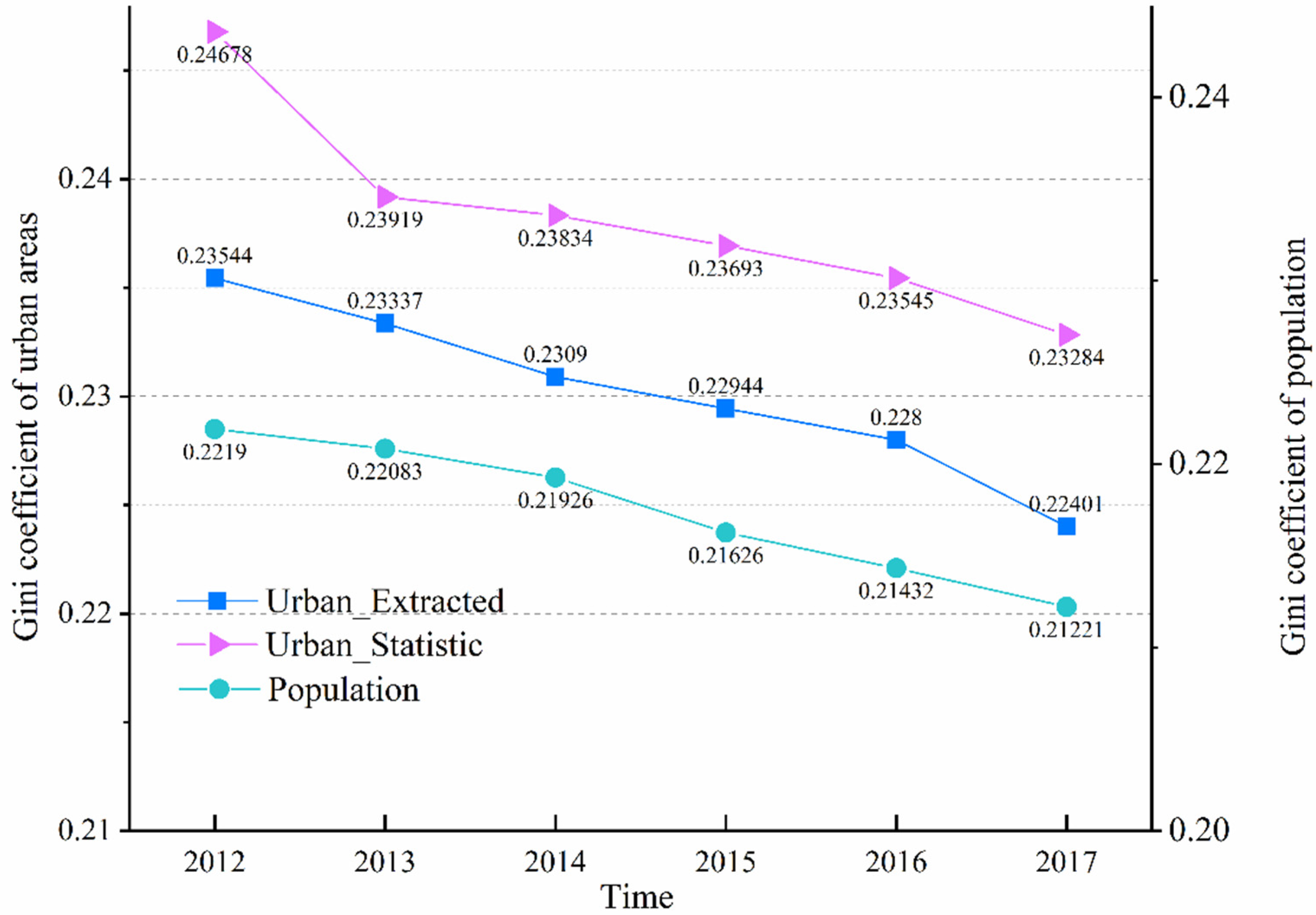
3.2.3. Variations in the Gini Coefficient
3.3. Sensitive Analysis
3.4. Comparison with Other Results
4. Conclusions
Author Contributions
Funding
Conflicts of Interest
References
- Schneider, A.; Friedl, M.A.; Potere, D. Mapping global urban areas using MODIS 500-m data: New methods and datasets based on ‘urban ecoregions’. Remote Sens. Environ. 2010, 114, 1733–1746. [Google Scholar] [CrossRef]
- United Nations. World Urbanization Prospects: The 2014 Revisio. Available online: https://population.un.org/wup/publications/files/wup2014-report.pdf (accessed on 15 May 2020).
- Muhammad, S.; Lean, H.H. Does Financial Development Increase Energy Consumption? The Role of In-dustrialization and Urbanization in Tunisia. Energy Policy 2012, 40, 473–479. [Google Scholar]
- Walsh, C.J. Urban Impacts on the Ecology of Receiving Waters: A Framework for Assessment, Conservation and Restoration. Hydrobiologia 2000, 2, 107–114. [Google Scholar] [CrossRef]
- Kalnay, E.; Cai, M. Impact of urbanization and land-use change on climate. Nature 2003, 423, 528–531. [Google Scholar] [CrossRef] [PubMed]
- Weng, Q.; Firozjaei, M.K.; Sedighi, A.; Kiavarz, M.; Alavipanah, S.K. Statistical analysis of surface urban heat island intensity variations: A case study of Babol city, Iran. GIScience Remote Sens. 2018, 56, 576–604. [Google Scholar] [CrossRef]
- Zipf, G.K. Human Behavior and the Principle of Least Effort: An Introduction to Human Ecology; Addison-Wesley: New York, NY, USA, 1949. [Google Scholar]
- Mark, J. The Law of the Primate City. Geogr. Rev. 1939, 2, 226–232. [Google Scholar]
- Gini, C. Measurement of Inequality of Incomes. Econ. J. 1921, 31, 124. [Google Scholar] [CrossRef]
- Huang, Q.; He, C.; Gao, B.; Yang, Y.; Liu, Z.; Zhao, Y.; Dou, Y. Detecting the 20 year city-size dynamics in China with a rank clock approach and DMSP/OLS nighttime data. Landsc. Urban Plan. 2015, 137, 138–148. [Google Scholar] [CrossRef]
- Anderson, G.; Ying, G. The Size Distribution of Chinese Cities. Reg. Sci. Urban Econ. 2005, 6, 756–776. [Google Scholar] [CrossRef]
- Fan, C.C. The Vertical and Horizontal Expansions of China’s City System. Urban Geogr. 1999, 6, 493–515. [Google Scholar] [CrossRef]
- Xu, Z.; Zhu, N. City Size Distribution in China: Are Large Cities Dominant? Urban Stud. 2009, 10, 2159–2185. [Google Scholar] [CrossRef] [Green Version]
- Levin, N.; Zhang, Q. A global analysis of factors controlling VIIRS nighttime light levels from densely populated areas. Remote Sens. Environ. 2017, 190, 366–382. [Google Scholar] [CrossRef] [Green Version]
- Yao, Y.; Chen, D.; Chen, L.; Wang, H.; Guan, Q. A time series of urban extent in China using DSMP/OLS nighttime light data. PLoS ONE 2018, 13, e0198189. [Google Scholar] [CrossRef] [Green Version]
- Zou, Y.; Peng, H.; Liu, G.; Yang, K.; Xie, Y.; Weng, Q. Monitoring Urban Clusters Expansion in the Middle Reaches of the Yangtze River, China, Using Time-Series Nighttime Light Images. Remote Sens. 2017, 10, 1007. [Google Scholar] [CrossRef] [Green Version]
- Nitsch, V. Zipf Zipped. J. Urban Econ. 2005, 1, 86–100. [Google Scholar] [CrossRef]
- Fu, Y.; Li, J.; Weng, Q.; Zheng, Q.; Li, L.; Dai, S.; Guo, B. Characterizing the spatial pattern of annual urban growth by using time series Landsat imagery. Sci. Total Environ. 2019, 666, 274–284. [Google Scholar] [CrossRef]
- Huang, X.; Schneider, A.; Friedl, M.A. Mapping sub-pixel urban expansion in China using MODIS and DMSP/OLS nighttime lights. Remote Sens. Environ. 2016, 175, 92–108. [Google Scholar] [CrossRef]
- Xie, Y.; Weng, Q.; Fu, P. Temporal Variations of Artificial Nighttime Lights and Their Implications for Ur-banization in the Conterminous United States, 2013–2017. Remote Sens. Environ. 2019, 225, 160–174. [Google Scholar] [CrossRef]
- Yu, B.; Shu, S.; Liu, H.; Song, W.; Wu, J.; Wang, L.; Chen, Z. Object-based spatial cluster analysis of urban landscape pattern using nighttime light satellite images: A case study of China. Int. J. Geogr. Inf. Sci. 2014, 28, 2328–2355. [Google Scholar] [CrossRef]
- Su, Y.; Chen, X.; Wang, C.; Zhang, H.; Liao, J.; Ye, Y.; Wang, C. A new method for extracting built-up urban areas using DMSP-OLS nighttime stable lights: A case study in the Pearl River Delta, southern China. GIScience Remote Sens. 2015, 52, 218–238. [Google Scholar] [CrossRef]
- Small, C.; Elvidge, C.D. Night on Earth: Mapping Decadal Changes of Anthropogenic Night Light in Asia. Int. J. Appl. Earth Obs. Geoinf. 2013, 22, 40–52. [Google Scholar] [CrossRef] [Green Version]
- Small, C.; Elvidge, C.D.; Balk, D.; Montgomery, M. Spatial scaling of stable night lights. Remote Sens. Environ. 2011, 115, 269–280. [Google Scholar] [CrossRef]
- Elvidge, C.D.; Baugh, K.E.; Zhizhin, M.; Hsu, F.-C. Why VIIRS data are superior to DMSP for mapping nighttime lights. Proc. Asia-Pac. Adv. Netw. 2013, 35, 62. [Google Scholar] [CrossRef] [Green Version]
- Miller, S.D.; Straka, W.; Mills, S.P.; Elvidge, C.D.; Lee, T.F.; Solbrig, J.; Walther, A.; Heidinger, A.K.; Weiss, S.C. Illuminating the Capabilities of the Suomi National Polar-Orbiting Partnership (NPP) Visible Infrared Imaging Radiometer Suite (VIIRS) Day/Night Band. Remote Sens. 2013, 5, 6717–6766. [Google Scholar] [CrossRef] [Green Version]
- Cao, C.; Bai, Y. Quantitative Analysis of VIIRS DNB Nightlight Point Source for Light Power Estimation and Stability Monitoring. Remote Sens. 2014, 6, 11915–11935. [Google Scholar] [CrossRef] [Green Version]
- Zhou, Y.; Smith, S.J.; Elvidge, C.D.; Zhao, K.; Thomson, A.; Imhoff, M. A cluster-based method to map urban area from DMSP/OLS nightlights. Remote Sens. Environ. 2014, 147, 173–185. [Google Scholar] [CrossRef]
- Xie, Y.; Weng, Q. Updating Urban Extents with Nighttime Light Imagery by Using an Object-Based Thresh-olding Method. Remote Sens. Environ. 2016, 187, 1–13. [Google Scholar] [CrossRef]
- Henderson, M.; Yeh, E.; Gong, P.; Elvidge, C.; Baugh, K. Validation of urban boundaries derived from global night-time satellite imagery. Int. J. Remote Sens. 2003, 24, 595–609. [Google Scholar] [CrossRef]
- Liu, Z.; He, C.; Zhang, Q.; Huang, Q.; Yang, Y. Extracting the dynamics of urban expansion in China using DMSP-OLS nighttime light data from 1992 to 2008. Landsc. Urban Plan. 2012, 106, 62–72. [Google Scholar] [CrossRef]
- Ma, T.; Zhou, Y.; Zhou, C.; Haynie, S.; Pei, T.; Xu, T. Night-Time Light Derived Estimation of Spa-tio-Temporal Characteristics of Urbanization Dynamics Using Dmsp/Ols Satellite Data. Remote Sens. Environ. 2015, 158, 453–464. [Google Scholar] [CrossRef]
- Cao, X.; Chen, J.; Imura, H.; Higashi, O. A SVM-based method to extract urban areas from DMSP-OLS and SPOT VGT data. Remote Sens. Environ. 2009, 113, 2205–2209. [Google Scholar] [CrossRef]
- Jing, W.; Yang, Y.; Yue, X.; Zhao, X. Mapping Urban Areas with Integration of DMSP/OLS Nighttime Light and MODIS Data Using Machine Learning Techniques. Remote. Sens. 2015, 7, 12419–12439. [Google Scholar] [CrossRef] [Green Version]
- Xu, T.; Coco, G.; Gao, J. Extraction of urban built-up areas from nighttime lights using artificial neural network. Geocarto Int. 2019, 35, 1049–1066. [Google Scholar] [CrossRef]
- Lu, D.; Tian, H.; Zhou, G.; Ge, H. Regional mapping of human settlements in southeastern China with multisensor remotely sensed data. Remote Sens. Environ. 2008, 112, 3668–3679. [Google Scholar] [CrossRef]
- Yang, Y.; He, C.; Zhang, Q.; Han, L.; Du, S. Timely and accurate national-scale mapping of urban land in China using Defense Meteorological Satellite Program’s Operational Linescan System nighttime stable light data. J. Appl. Remote Sens. 2013, 7, 073535. [Google Scholar] [CrossRef]
- Kubat, M.; Holte, R.C.; Matwin, S. Machine Learning for the Detection of Oil Spills in Satellite Radar Images. Mach. Learn. 1998, 30, 195–215. [Google Scholar] [CrossRef] [Green Version]


| Data | Description | Resolution | Time |
|---|---|---|---|
| NPP VIIRS | Night-time light | 500 m/Month | |
| MOD 13A1 | Normalized Differential Vegetation Index | 500 m/16 Days | 2012–2017 |
| MOD 11A2 | Land-surface temperature | 1 km/8 Days | |
| MOD 44w | Global land water mask | 250 m/Year | 2012–2017 |
| MCD 12Q1 | Land-cover type | 500 m/Year | 2012–2017 |
| Population | Year | 2012–2017 | |
| Statistical urban areas | 0.01 km2 | 2012–2017 |
| Accuracy | 2012 | 2013 | 2014 | 2015 | 2016 | 2017 |
|---|---|---|---|---|---|---|
| g-mean (%) | 82.10 | 84.88 | 83.06 | 79.21 | 83.94 | 84.10 |
| Kappa | 0.793 | 0.828 | 0.805 | 0.761 | 0.816 | 0.817 |
| Year | Urban Areas | Population | ||
|---|---|---|---|---|
| Fitting Equations | R2 | Fitting Equations | R2 | |
| 2012 | y = −1.048x + 3.782 | 0.796 | y = −0.884x + 3.347 | 0.840 |
| 2013 | y = −1.034x + 3.784 | 0.801 | y = −0.880x + 3.352 | 0.838 |
| 2014 | y = −1.019x + 3.784 | 0.795 | y = −0.875x + 3.357 | 0.835 |
| 2015 | y = −1.008x + 3.788 | 0.798 | y = −0.856x + 3.351 | 0.860 |
| 2016 | y = −1.010x + 3.793 | 0.797 | y = −0.852x + 3.357 | 0.860 |
| 2017 | y = −0.982x + 3.791 | 0.789 | y = −0.845x + 3.361 | 0.858 |
Publisher’s Note: MDPI stays neutral with regard to jurisdictional claims in published maps and institutional affiliations. |
© 2022 by the authors. Licensee MDPI, Basel, Switzerland. This article is an open access article distributed under the terms and conditions of the Creative Commons Attribution (CC BY) license (https://creativecommons.org/licenses/by/4.0/).
Share and Cite
Ding, Y.; Hu, J.; Yang, Y.; Ma, W.; Jiang, S.; Pan, X.; Zhang, Y.; Zhu, J.; Cao, K. Monitoring the Distribution and Variations of City Size Based on Night-Time Light Remote Sensing: A Case Study in the Yangtze River Delta of China. Remote Sens. 2022, 14, 3403. https://doi.org/10.3390/rs14143403
Ding Y, Hu J, Yang Y, Ma W, Jiang S, Pan X, Zhang Y, Zhu J, Cao K. Monitoring the Distribution and Variations of City Size Based on Night-Time Light Remote Sensing: A Case Study in the Yangtze River Delta of China. Remote Sensing. 2022; 14(14):3403. https://doi.org/10.3390/rs14143403
Chicago/Turabian StyleDing, Yuan, Jia Hu, Yingbao Yang, Wenyu Ma, Songxiu Jiang, Xin Pan, Yong Zhang, Jingjing Zhu, and Kai Cao. 2022. "Monitoring the Distribution and Variations of City Size Based on Night-Time Light Remote Sensing: A Case Study in the Yangtze River Delta of China" Remote Sensing 14, no. 14: 3403. https://doi.org/10.3390/rs14143403