An Impervious Surface Spectral Index on Multispectral Imagery Using Visible and Near-Infrared Bands

Abstract

The accurate mapping of urban impervious surfaces from remote sensing images is crucial for understanding urban land-cover change and addressing impervious-surface-change-related environment issues. To date, the authors of most studies have built indices to map impervious surfaces based on shortwave infrared (SWIR) or thermal infrared (TIR) bands from middle–low-spatial-resolution remote sensing images. However, this limits the use of high-spatial-resolution remote sensing data (e.g., GaoFen-2, Quickbird, and IKONOS). In addition, the separation of bare soil and impervious surfaces has not been effectively solved. In this article, on the basis of the spectra analysis of impervious surface and non-impervious surface (vegetation, water, soil and non-photosynthetic vegetation (NPV)) data acquired from world-recognized spectral libraries and Sentinel-2 MSI images in different regions and seasons, a novel spectral index named the Normalized Impervious Surface Index (NISI) was proposed for extracting impervious area information by using blue, green, red and near-infrared (NIR) bands. We performed comprehensive assessments for the NISI, and the results demonstrated that the NISI provided the best studied performance in separating the soil and impervious surfaces from Sentinel-2 MSI images. Furthermore, regarding impervious surfaces mapping accuracy, the NISI had an overall accuracy (OA) of 89.28% (±0.258), a producer’s accuracy (PA) of 89.76% (±1.754), and a user’s accuracy (UA) of 90.68% (±1.309), which were higher than those of machine learning algorithms, thus supporting the NISI as an effective measurement for urban impervious surfaces mapping and analysis. The results indicate the NISI has a high robustness and a good applicability.

1. Introduction

Impervious surfaces are man-made land surface features through which water cannot infiltrate, e.g., paved roads, driveways, sidewalks, parking lots, and rooftops [1]. In recent years, impervious surfaces have become not only the most prominent feature of urbanization but also one of the major contributors to the environmental impacts caused by urbanization [2]. The change of natural or semi-natural surfaces into impervious surfaces (roads, parking lots, buildings, etc.) impacts the radiation budget, resulting in an increase in the local surface and air temperatures [3,4,5]. In addition, the increasing amounts of impervious surfaces may also disrupt the recharge of underground water and increase the risk of flooding [6]. Therefore, the timely and accurate acquisition of urban impervious surface information is of great significance for promoting sustainable urban development in human activities.

Increasingly rich remote sensing datasets have drawn considerable attention in recent years to impervious surface information extraction based on remote sensing technology [7]. In the past, extracting impervious surface information was difficult because land use exhibits nonlinearity and spatial heterogeneity caused by complex interactions between the ecological environment and socioeconomic status [8,9]. Currently, remote sensing methods for studying impervious surfaces fall into four main categories: (1) spectral mixture analysis [10,11,12], (2) regression model [13,14], (3) machine learning methods [15,16,17], and (4) spectral indices [18,19,20].

Spectral mixture analysis (SMA) includes linear, nonlinear, and normalized spectral mixture analysis algorithms [11,21,22]. A large number of mixed pixels are in low-resolution images due to the spatial heterogeneity and fragmentation of the ground objects. Appropriate endmember selection is a critical step for the success of SMA [23]. The vegetation-impervious surface-soil (V-I-S) model has become an accepted alternative to parameterize the biophysical composition of urban environments [11,24]. Although SMA-based methods have shown some success in mapping a fraction of impervious surfaces, it is difficult to obtain a certain number of pure endmembers due to the insufficient utilization of details of impervious surfaces when applied to medium- and low-spatial-resolution remote sensing data, which may lead to decreases in accuracy [25]. In urban environments, regression model training fully depends on the availability of stable and comparable surface reflectance units between images and comprehensive training information [15]. For example, Okujeni et al [13] used support vector regression and synthetically mixed training data to quantify urban land cover. They demonstrated the potential of the regression model for the quantitative mapping of four spectrally complex and ecologically meaningful urban land-cover types on a purely spectral basis. Machine learning methods such as decision trees [26], neural networks [27], support vector machines (SVMs) [28], and random forests (RFs) [29] have been commonly used for impervious surface detection during the past few decades. These methods build knowledge by learning prior information and modifying knowledge bases via the self-learning of training samples and test samples. They can also complete self-cognition and environmental cognition tasks. Despite the effectiveness of these methods, many challenges still exist, including the impacts of atmospheric correction, the usage of multitemporal images, susceptibility to human intervention, and high operating costs in the process of classification [30]. Compared to the three above-mentioned methods, the spectral index-based impervious surface information extraction method is relatively simple and efficient.

Many researchers have proposed efficient and relatively simple methods based on spectral indices to map urban impervious surfaces [31]. With the spectral features of impervious surfaces provided by such spectral indices, impervious surfaces can be automatically and rapidly identified over large areas. Spectral indices commonly used to identify impervious surfaces include the Biophysical Composition Index (BCI) [18], the Normalized Difference Built-up Index (NDBI) [32], the Index-based Built-up Index (IBI) [31], and the Normalized Difference Impervious Surface Index (NDISI) [33]. Wang & Li [34] proposed the urban impervious surfaces index (UISI), which was shown to outperform the existing Genetic Algorithm-based Urban Cluster Automatic Threshold (GA-UCAT) and the Gaussian-based Automatic Threshold Modified Normalized Difference Impervious Surface Index (G-MNDISI) by an average increase of 6.51% in overall accuracy. Even though these indices have been found to be effective to some degree when used to extract impervious surface information, several problems still exist. Firstly, current impervious surface indices commonly use SWIR or TIR bands, thus limiting the application of many high-spatial-resolution-images lacking SWIR or TIR bands such as GF-2, Quickbird, and IKONOS. These images can provide much finer spatial resolution information, which is important for detailed impervious surface identification and feature application [35]. Secondly, the applicability of these indices in varied seasons, which could influence the results of urban impervious surface mapping, is unclear. Finally, a spectral index is constructed by using the spectral difference between impervious and non-impervious features. However, the spectra of low-albedo man-made materials can be similar to those of bare soil, leading to a mixture of pixels and a lower extraction accuracy [20,36]. Therefore, there is an urgent need to develop a novel method relying on sole visible and near-infrared multispectral bands to support the automated mapping of impervious surfaces in urban areas.

To support this need, we proposed a new spectral index for identifying impervious surfaces. The spectral index, called the Normalized Impervious Surface Index (NISI), combines the spectral characteristics of different ground objects in urban areas and only uses the four common blue, green, red and near-infrared bands. Therefore, the spectral index lifts the limitation of the lack of SWIR and TIR bands for high-spatial-resolution images. In addition, the NISI is also able to distinguish impervious surfaces from bare soil.

The remainder of this article is organized as follows. Section 2 introduces the study area and data. Section 3 presents the methodology of the NISI development, including spectral analysis and the formulation of the NISI. The results of the NISI and comparisons with other indices and methods are reported in Section 4. Finally, discussion and conclusions are provided in Section 5 and Section 6.

2. Study Areas and Data

2.1. Study Area

In this study, we chose three representative cities of China with different regions, Beijing, Nanjing, and Guangzhou, to test the NISI extraction model. The three cities, having varied climate conditions and economic development features, were chosen to ensure the feasibility of the proposed model.

Beijing (39°24′–41°36′N, 115°42′–117°24′E) is the largest city in China and one of the most developed cities in the world. It is located in North China and is the core city of the Beijing–Tianjin–Hebei Region city cluster. The local temperate monsoon climate yields a cold and dry winter and a hot and rainy summer. Beijing has a total area of 16,410 km², including 1401 km² of built-up area cover. The population of permanent residents was 21.886 million and the urbanization rate was 87.5% in 2021.

Nanjing (31°14′–32°37′N, 118°22′–119°14′E) is located in the core city of the Yangtze River Delta city cluster, East China. Its mild winter and hot and humid summer are features of its subtropical monsoon climate. Nanjing has a total area of 6587.02 km², including a built-up area of 817.38 km². The population of permanent residents was 9.423 million and the urbanization rate was 86.9% in 2021.

Guangzhou (22°26′–23°56′N, 112°57′–114°3′E) is located in the core city of the Pearl River Delta city cluster, South China. Th marine subtropical monsoon climate yields a non-distinction of seasons features. Guangzhou has a total area of 7434.4 km², including a built-up area of 1300.01 km². The population of permanent residents was 18.811 million and the urbanization rate was 86.46% in 2021.The three areas are densely developed, with large populations and various land-cover types; the locations of three cities are shown in Figure 1.

2.2. Data and Pre-Processing

2.2.1. Remote Sensing Image Data

In this study, we gathered Sentinel-2 imagery in different areas and seasons. The influence of urban shadow, vegetation coverage and bare soil exposure on impervious surfaces was obvious between southern and northern cities in different seasons, so the images are discussed in different seasons: spring (March–May), summer (June–August), autumn (September–November), and winter (December–February).

Sentinel-2 Multispectral Instrument (MSI) imagery with high pixel quality and low cloud cover (<10%) was selected and downloaded from the European Space Agency (ESA) ScienceHub and the Google Earth Engine (GEE) (https://code.earthengine.google.com/, accessed on 21 September 2021). The product level of the used Sentinel-2 images is Level 2A, which provides bottom of atmosphere (BOA) reflectance data. Each Level-2A product covers 100 × 100 km² in cartographic geometry (UTM/WGS84 projection). To enable comparison to other indices in each study area, the SWIR bands (band 11 and band 12) were resampled to a spatial resolution of 10 m using bilinear interpolation in the software ESA SNAP (Sentinel Application Platform, version 8.0, European Space Agency, http://step.esa.int/main/download/, accessed on 30 September 2021). Detailed descriptions of the image acquisition time and band information are provided in

Table 1. Specifications of Sentinel-2 images for the three cities considered in the study.

Study Area	Season	Data	Acquisition Time	Cloud Coverage (%)	Product Level
Beijing	Winter	16 February 2021	03:08:11	6.24	L2A
	Spring	2 May 2021	03:05:39	1.75	L2A
	Summer	10 August 2021	03:05:49	0.58	L2A
	Autumn	13 November 2020	03:09:59	1.01	L2A
Nanjing	Winter	20 February 2021	02:47:31	0.51	L2A
	Spring	1 May 2021	02:45:41	0.88	L2A
	Summer	30 July 2021	02:45:51	1.19	L2A
	Autumn	7 November 2020	02:49:19	0.40	L2A
Guangzhou	Winter	1 December 2019	03:01:01	2.53	L2A
	Spring	30 January 2020	02:59:41	3.20	L2A
	Summer	22 September 2019	02:55:41	3.38	L2A
	Autumn	21 November 2019	03:00:21	2.87	L2A

and

Table 2. Characteristics of Sentinel-2A bands.

Band Name	Wavelength (nm)	Central Wavelength (nm)	Bandwidth (nm)	Spatial Resolution (m)
Band 2 (Blue)	458–523	496.6	65	10
Band 3 (Green)	543–578	560.0	35	10
Band 4 (Red)	650–680	664.5	20	10
Band 8 (NIR)	785–900	835.1	115	10
Band 11 (SWIR-1)	1565–1655	1613.7	90	20
Band 12 (SWIR-2)	2100–2280	2202.4	180	20

, and the reasons for band selection are described in Section 3.

2.2.2. Laboratory Data

To compare the spectral differences between impervious and non-impervious surfaces, multiple spectra covering visible to shortwave infrared (400–2500 nm) waves were selected from the ECOSTRESS spectral library (https://speclib.jpl.nasa.gov/library, accessed on 13 July 2021). The spectral library contains 72 man-made object spectra, 122 NPV spectra, 69 soil spectra, 1037 vegetation spectra, and 9 water spectra. Ten impervious materials were selected: metal, roofing paper, roofing shingle, rubber, shingle, tile, paving concrete, construction concrete, brick, and marble. In addition, four non-impervious material were selected: water, soil, vegetation, and NPV. NPV means dead and senescent vegetation, as well as non-photosynthesizing branch and stem tissues, and it is an essential component in various vegetation-soil ecosystems including agricultural areas, forests, and grasslands [37,38].

3. Methodology

3.1. Normalized Difference Impervious Surface Index (NISI)

When quantifying and mapping impervious surfaces in urban areas, it is important to understand the spectral features of impervious materials. We found that the reflectance of different material types was highly diverse in both shape and magnitude by analyzing the spectral curves of typical impervious surface materials in the spectral library (Figure 2a). To better understand the performance of the typical impervious surface material spectrum in the Sentinel-2A MSI remote sensing data, the spectral curves of typical impervious surface materials were resampled based on the spectral response function of the Sentinel-2A MSI sensors provided by the ESA, as shown as in Figure 2b.

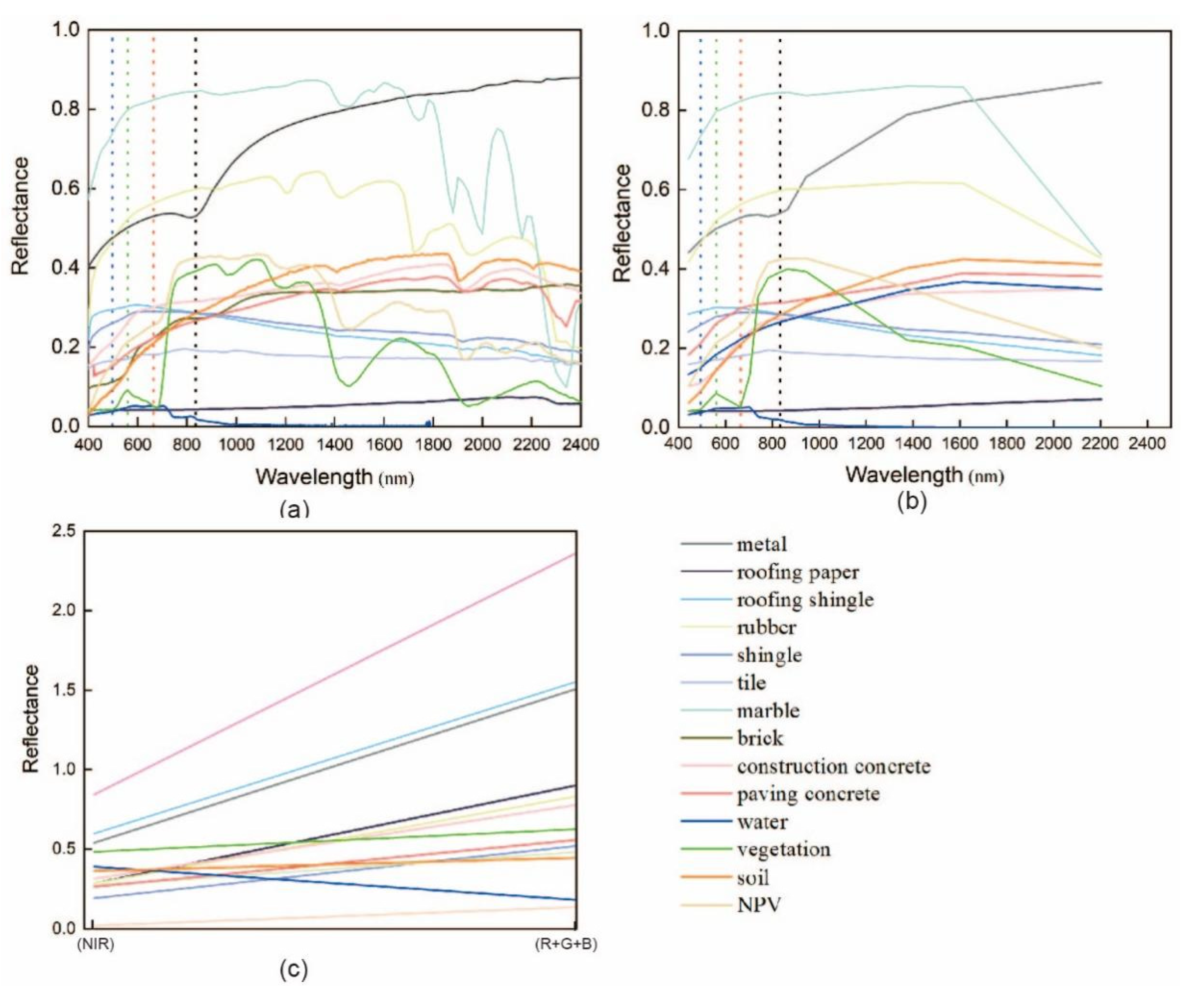
3.1.1. Analysis of Spectral Reflectance Curves of Different Ground Objects

As shown as in Figure 2b, metal, rubber, and marble were found to have relatively high spectral reflectance values, whereas the spectral reflectance values of other impervious materials (e.g., roofing shingle, paving asphalt, and brick) were comparatively lower and featureless in the visible range. Furthermore, the reflectance values of soil and NPV in the visible range were higher. Additionally, the reflectance values of impervious ground objects were similar in the visible range and the NIR range. In contrast, the reflectance values of vegetation were much higher in the NIR than the visible range. Furthermore, Figure 2b also shows that water had almost zero reflectance in the NIR range, whereas other ground objects had nonzero reflectance in the NIR range. In addition, the reflectance values of soil and NPV in NIR were higher than in the blue and green range, so the reflectance value difference between the visible and NIR ranges of soil and NPV was smaller than those of impervious ground objects.

3.1.2. Spectral Analysis of Typical Objects within Urban Areas

To analyze the spectra features of typical urban objects, Sentinel-2 images from different seasons were selected. The land-cover types were divided into five classes in urban areas: (1) high-albedo impervious objects (e.g., metal, rubber, and marble); (2) low-albedo impervious objects (e.g., roofing shingle, paving asphalt, and brick); (3) bare soil and NPV (e.g., dry grass and leaves)—in this paper, due to similar spectral curves, the bare soil and NPV were not distinguished; (4) vegetation (e.g., grassland, urban green belt, and farmland); and (5) water (e.g., lakes and reservoir), in which classes (3)–(5) were classified as non-impervious surfaces.

Then, we compared the spectral reflectance of the same land-cover region across different bands of multitemporal images (see Figure 3). First, we selected vegetation, water, bare soil, high-albedo impervious surfaces and low-albedo impervious surface pixels from Sentinel-2 MSI images in three areas during the four seasons, and about 2000 pixels were selected for each land-cover type. Then we calculated the mean and standard deviation of the reflectance of each type of land cover in each band. Figure 3 shows that the reflectance of the same land-cover varied when season cycling at all bands. More specifically, the reflectance of high-albedo impervious objects was found to be higher than other non-impervious objects. The soil and NPV reflectance values were similar to that of low-albedo impervious objects. The reflectance values of water and vegetation showed subtle changes with seasonal changes. Figure 3a presents the seasonal spectral reflectance of different land-cover types in Beijing from Sentinel-2A MSI imagery. The increased reflectance rates of soil and NPV in spring and summer were higher than those in winter and autumn, possibly because vegetation was dominant in spring and summer. The reflectance of high-albedo and low-albedo impervious slightly varied in the visible and NIR bands in different seasons. The low-albedo impervious objects were shown to have low and featureless reflectance in the visible and NIR bands.

Figure 3b presents the seasonal spectral reflectance values of different land-cover types in Nanjing from Sentinel-2 MSI imagery. The reflectance of water and vegetation significantly varied in different seasons. The vegetation reflectance in spring and summer was higher than that in autumn and winter for the NIR band due to the leaf structures of the vegetation. Figure 3c presents the seasonal spectral reflectance values of different land-cover types in Guangzhou from Sentinel-2 MSI image. Guangzhou has a subtropical monsoon climate, so the spectral curves of urban features in different seasons had little fluctuation. The reflectance of high-albedo and low-albedo impervious objects was featureless. The spectral reflectance of all urban ground objects was observed to vary across seasons and locations. This was attributed to the north–south latitudinal difference in the three cities.

3.1.3. The Development of NISI

Based on the spectral analysis discussed above, we calculated both the sum and the difference between the visible and NIR reflectance (Figure 2c). It was found that the ratio between the difference and sum of the reflectance of impervious surfaces in the visible and NIR bands was greater than that of bare soil, NPV, and vegetation.

Various normalized difference indices have been developed and intensively used since the development of the NDVI [33]. Thus, we proposed the Normalized difference visible–NIR impervious surface index (NISI) using visible and NIR bands to map the impervious surfaces in urban areas:

$$NISI=\frac{\left(B_{blue}+B_{green}+B_{red}\right)-B_{NIR}}{\left(B_{blue}+B_{green}+B_{red}\right)+B_{NIR}}$$

(1)

where the B_blue, B_green, B_red, and B_NIR values of the Sentinel-2A data were set as 492.4 nm (band 2), 559.8 nm (band 3), 664.6 nm (band 4), and 832.8 nm (band 8), respectively. The NISI distinguishes impervious surface from non-impervious surface pixels according to the difference in the pixel gray scale after spectral band calculation.

3.2. Impervious Surface Mapping Based on NISI

The proposed NISI was used for urban impervious surface mapping for further validation. Our main goal was to determine the threshold between non-impervious and impervious surfaces. First, we obtained a frequency distribution histogram of an NISI image and calculated the first derivative of the differential value of 0 and set it as the initial threshold [39,40]. Then, a trial-and-error procedure based on F_pb [41] was adopted to determine the appropriate NISI threshold. Specifically, we labeled impervious surface pixels that could be identified in the Sentinel-2 MSI image at a 10 m resolution. Non-impervious surface samples were also randomly generated from the image and labeled. According to the sampling strategy described by Zhang and Li [42], a polygon area (approximately 500–1000 pixels) around each remaining pixel was selected as a non-impervious surface sample. In addition, unlabeled pixels were randomly selected from the image and are referred to as background pixels [41]. It should be noted that these background pixels could be impervious or non-impervious surfaces. In this method, F_pb is a proxy of the F-measure based on samples from the positive class (target class, impervious surfaces in this study) and the background class. For a specified threshold, the F_pb value for the corresponding mapping result was obtained. The threshold that produced the highest F_pb value was considered optimal. Detailed information is provided in the Appendix A. If more than one threshold value produced similar-to-high F_pb values, the threshold that generated more balanced producer’s accuracy (PA) and user’s accuracy (UA) values was adopted [43]. Specifically, if the NISI value of a pixel was larger than the specified threshold value, the pixel was identified as an impervious surface. Otherwise, the pixel was identified as non-impervious surface. For comparison, the same thresholding method was used to create NDBI, BCI, UI, and IBI maps of impervious surfaces.

$$NDBI=\frac{SWI{R}_1-NIR}{SWI{R}_1+NIR},$$

(2)

$$BCI=\frac{\left(H+L\right)/2-V}{\left(H+L\right)/2+V},$$

(3)

$$H=\frac{TC1-TC{1}_{min}}{TC{I}_{max}-TC{I}_{min}},$$

(4)

$$V=\frac{TC2-TC{2}_{min}}{TC{2}_{max}-TC{2}_{min}},$$

(5)

$$L=\frac{TC3-TC{3}_{min}}{TC{3}_{max}-TC{3}_{min}},$$

(6)

$$UI=\frac{SWI{R}_2-NIR}{SWI{R}_2+NIR},$$

(7)

$$IBI=\frac{\frac{2SWI{R}_1}{SWI{R}_1+NIR}-\left(\frac{NIR}{NIR+Red}+\frac{Green}{Green+SWI{R}_1}\right)}{\frac{2SWI{R}_1}{SWI{R}_1+NIR}+\left(\frac{NIR}{NIR+Red}+\frac{Green}{Green+SWI{R}_1}\right)}$$

(8)

where Green, Red, NIR, SWIR1, and SWIR2 correspond to band 2, band 4, band 8, band 11, and band 12, respectively. Thus, TCi (i = 1, 2, 3) indicates component I of the tasseled cap transformation (TC). The coefficients of Sentinel-2 tasseled cap transformation was set in reference to Nedkov’s work [44].

3.3. Separability Analysis between Impervious Surface and Bare Soil

Bare soil is a key disturbance factor influencing the effectiveness of the NISI model. Due to seasonal land-cover changes and their inherent mixtures with vegetation, bare soil and low-albedo impervious surfaces could not be accurately quantified from the remote sensing images [11,18]. In order to more directly display the separation degree of the NISI on bare soil and impervious surfaces, remote sensing images containing more bare soil were needed, and a Sentinel-2 MSI image of Beijing on 13 November 2020 was consequently selected. Because there is a large amount of vegetation that dries up and leads to more soil exposure in Beijing during late autumn, we chose an image of an area near the Beijing International airport where bare soil, vegetation, water, and impervious surfaces are abundant.

We selected the NDBI, BCI, UI, and IBI for comparison to the NISI to investigate and quantify the separability between pure pixels of bare soil and impervious surfaces by visually examining their histograms using three methods: (i) the spectral discrimination index (SDI), (ii) the transformed divergence (TD), and (iii) the Bhattacharyya distance (B-distance). The SDI is an indicator to evaluate the degree of separation between two land-cover histograms [45]. It is calculated by dividing the absolute value of the differences between the mean index values of the two land-cover types by the sum of their standard deviations [46]:

$$SDI=\frac{\left|{\mu }_1-{\mu }_2\right|}{{\sigma }_1+{\sigma }_2}$$

(9)

where μ₁ and μ₂ are the mean indices of land-cover types 1 and 2, respectively, and σ₁ and σ₂ are the standard deviations of the indices associated with land-cover types 1 and 2, respectively.

The TD measures separability via a saturating function of divergence [18,43,47]. The B-distance is originally defined as measuring the statistical distance between two Gaussian distributions and is now widely used for quantitative spectral separability in remote sensing applications [48]. A greater SDI value indicates that the two land-cover types can be effectively separated, while a lower SDI value indicates spectral mixture. As a rule of thumb, an SDI value greater than unity indicates satisfactory separability [49,50]. In addition to the SDI, the B-distance and TD are also separability indicators. Specifically, the TD indicates the separability between two classes, so TD < 1.7 indicates that two classes are poorly separable and TD > 1.9 indicates strong separability. Finally, 1.7 < TD < 1.9 means that the two classes are moderately separable [18,43]. No threshold exists for the B-distance; a greater B-distance simply corresponds to a higher degree of separation between two surfaces [10].

3.4. Accuracy Evaluation Method

Relative accuracy was identified using an accuracy verification approach in which a more accurate algorithm was used as the comparison object. Specifically, we selected RF, SVM, and CART classifiers for land-cover classification based on the Sentinel-2 data of Beijing (20210810), Nanjing (20210730), and Guangzhou (20190922) in the Google Earth Engine (GEE). The accuracy of classification results was compared to that of the proposed method. RF, SVM, and CART classifiers have been widely utilized in the remote sensing community for decades due to their excellent classification abilities in various large-scale land-cover mapping studies [27].

The false-color composites of Sentinel-2 MSI of Beijing, Nanjing, and Guangzhou were used to verify the accuracies of RF, SVM, CART, and the NISI. Random points were generated via stratified sampling, and 300 sample points were generated for each category. The attributes of sample points were determined through visual interpretation in ArcGIS, and the confusion matrix was calculated by point vector files after visual interpretation. The accuracy was measured using the OA, PA, and UA, which were calculated from a confusion matrix [43].

$$PA=\frac{N_a}{{{\displaystyle \sum }}_{i=1}^2{N}_{i1}}$$

(10)

$$UA=\frac{N_a}{{{\displaystyle \sum }}_{j=1}^2{N}_{1j}}$$

(11)

$$OA=\frac{{{\displaystyle \sum }}_{i=1}^2{N}_{ii}}{N}$$

(12)

where $N_a$ represents the number of pixels for positive validation samples and predictions, ${\displaystyle \sum }_{i=1}^2{N}_{i1}$ means the number of pixels whose validation samples were positive, ${\displaystyle \sum }_{j=1}^2{N}_{1j}$ means the number of pixels whose predictions are positive, and ${\displaystyle \sum }_{i=1}^2{N}_{ii}$ and N represent the number of correctly classified pixels and all the validation pixels, respectively.

4. Results

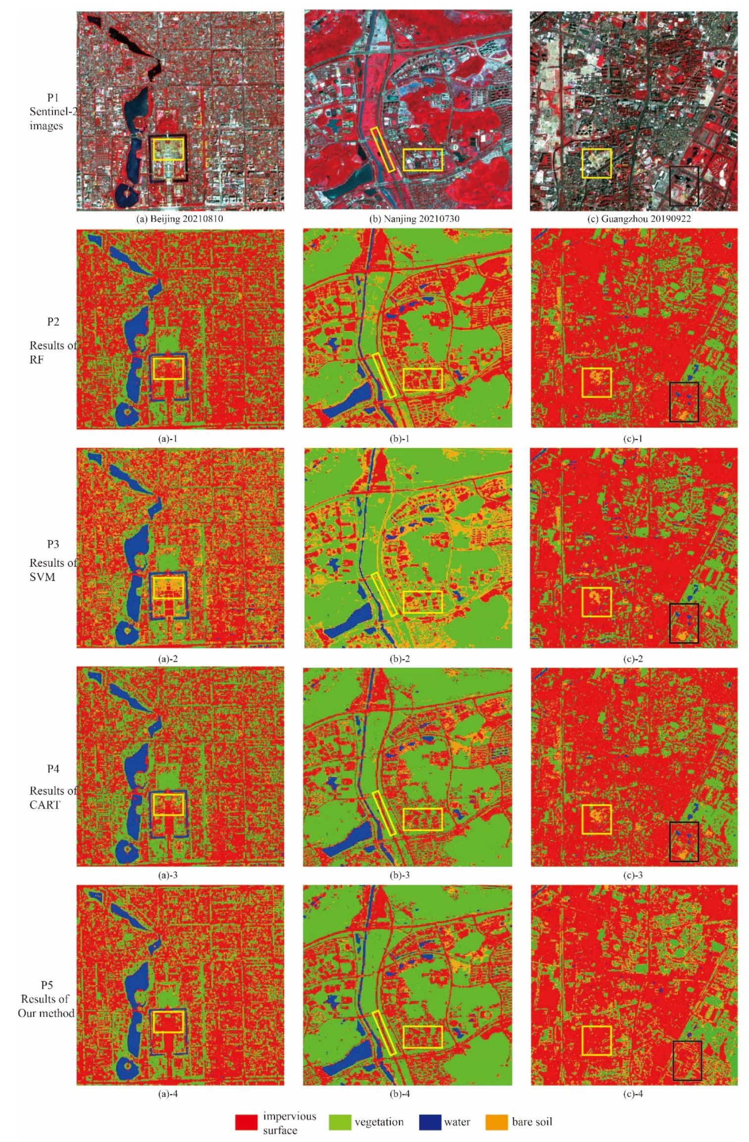
4.1. The Extraction of Impervious Surface Information via Index-Based Method

In Figure 4, the performance of the NISI model was verified using the multitemporal Sentinel-2 images from four seasons in the three study areas that were used for NISI image-generation using the threshold method described in Section 3.2. The gray values of the NISI varied with the seasons within the same urban area. The visual contrasts of various land-cover types were distinct in summer due to vegetation cover. For example, there were stronger contrast differences between impervious surfaces and non-impervious surfaces in summer in Nanjing and Beijing. However, due to the subtropical monsoon climate in Guangzhou, most vegetation remains green all year round, so there was no obvious difference in the grayscale rendering of the NISI in the four seasons. Water regions have high gray values in the NISI images, indicated by the white color, while the region of vegetation appeared with low gray values in the NISI images, and the bare soil and impervious surfaces were gray and light gray, respectively. The contrast between impervious surfaces and bare soil was significantly enhanced compared to the original images. During the extraction of impervious surface information, vegetation coverage could reduce the disturbance of bare soil, particularly during summer in mid-Northern China (Beijing and Nanjing), while in Southern China (Guangzhou), the vegetation coverage could reduce the disturbance of bare soil all year round because due the green vegetation in all four seasons.

Table 3. Average index values of four classes of land cover in NISI images derived from multitemporal Sentinel-2 images in Beijing, Nanjing, and Guangzhou, China.

City	The Classes of Land Cover	Winter	Spring	Summer	Autumn
Beijing	Water	0.6932	0.6235	0.6674	0.6561
	Impervious surface	0.3902	0.3728	0.4139	0.3872
	Bare soil and NPV	0.1931	0.1012	0.0054	0.2042
	Vegetation	−0.0253	−0.3234	−0.4206	0.0204
Nanjing	Water	0.7544	0.6968	0.7031	0.7357
	Impervious surface	0.3052	0.3418	0.3637	0.3316
	Bare soil and NPV	0.0826	0.0858	0.0875	0.1390
	Vegetation	−0.1593	−0.3222	−0.3376	−0.1582
Guangzhou	Water	0.7468	0.7599	0.7759	0.7689
	Impervious surface	0.4464	0.4234	0.4258	0.4433
	Bare soil and NPV	0.2381	0.2232	0.1992	0.2206
	Vegetation	−0.3846	−0.3788	−0.4391	−0.4211

shows the average index values of four land-cover classes derived from three areas and four seasons within the NISI images. The average index values of the four land-cover classes in three areas were different. For example, the average index value of water was around 0.67 in Beijing over the four seasons, while the average NISI values in Nanjing and Guangzhou were around 0.72 and 0.76, respectively. It was also found that the water quality of Beijing was slightly worse than that of Nanjing and Guangzhou. The average index value of impervious surfaces was around 0.3 in Nanjing over the four seasons, and the corresponding values were around 0.4 and 0.43 in Beijing and Guangzhou, respectively. The albedo and density of impervious surfaces affected the NISI values in the images. The NISI values of impervious surfaces with high albedo were higher than those of impervious surfaces with low albedo. However, the average NISI values of four land-cover classes had an apparent identifiable value range in the NISI image.

From Table 3, we found that the NISI values of bare soil and NPV remained around 0.21 all year around in Guangzhou, and the values greatly varied in Nanjing and Beijing with maxima of 0.14 and 0.20, respectively, in autumn. However, these values were all smaller than the NISI values for impervious surfaces and were well-discriminative. In addition, the degree of bare soil and NPV disturbance varied with the spatiotemporal changes due to vegetation cover. In Northern China, the main disturbance originated from uncultivated farmlands in autumn, though they were covered with vegetation in spring, summer and winter. However, in Southern China, most of the natural soil was covered by vegetation.

4.2. The Statistic Results of Separability Analysis

We selected the pixels of bare soil and impervious surfaces for comparisons of the frequency histograms of the NISI with other typical impervious surface indexes (NDBI, BCI, UI, and IBI) to show the separation degree of bare soil and impervious surfaces. The horizontal axis is the index value, and the vertical axis is the frequency of the index value in the index image. The yellow ellipses and red rectangles represent bare soil and impervious surfaces in Figure 5a–c, respectively. In Figure 5d, an obvious spectral mixture between bare soil and impervious surfaces can be discerned compared to the true-color Sentinel-2 MSI images. Upon further analysis, the UI histogram of impervious surfaces and bare soil (Figure 5h) indicated that, unlike the NISI, a significant mixture was observed between these two land-cover types. Notably, the UI values for impervious surfaces and bare soil wee similar, and their histograms had a wider range compared to the NISI. This observation was supported by lower values of SDI (0.52), TD (1.254), and B-distance (1.141). In summary, the UI image could not effectively separate impervious surfaces and bare soil with Sentinel-2 MSI images.

As seen in Figure 5f,g,i and

Table 4. Separability measures between impervious surfaces and bare soil with different indices.

Method	NISI	NDBI	BCI	UI	IBI
SDI	1.524	1.025	0.952	0.526	1.103
TD	1.928	1.712	1.701	1.254	1.724
B-distance	1.462	1.328	1.257	1.141	1.423

, some mixtures between bare soil and impervious surfaces were proven by the histogram analysis and the separability measures. In particular, the NDBI, BCI, and IBI showed moderate SDI, TD, and B-distance values, thus indicating a mixture between bare soil and impervious surfaces. However, no mixture between bare soil and impervious surfaces was proven by the histogram analysis (see Figure 5e) and the separability measures (see Table 4). In summary, the NISI more accurately distinguished between impervious surfaces and bare soil than the BCI, NDBI, UI, and IBI across all four separability measures.

4.3. The Impervious Surfaces Extraction Results of Machine Learning Methods

To evaluate the performance of our proposed method for land-cover mapping, we compared and analyzed the land-cover maps of three regions (selected from the three study areas: Beijing (20210810), Nanjing (20210730), and Guangzhou (20190922)) obtained by RF, SVM, CART and our proposed NISI method. We selected the Palace Museum in Beijing (see Figure 6a), Nanjing Xianlin University Town (see Figure 6b), and the area near the Children’ Park in Guangzhou (see Figure 6c) because the three regions contain high-density building areas, vegetation, water, and some bare soil. In the figure, the yellow polygon denotes some examples where our method outperformed RF, SVM, and CART. The black polygon denotes some examples where RF, SVM, and CART outperformed our method. The yellow polygon in Figure 6a is the Palace Museum, and the roof of the palace comprises yellow impervious surfaces, which were misclassified as bare soil by the RF, SVM, and CART methods (see Figure 6(a-1–a-3)) and correctly classified as impervious surfaces by our method (see Figure 6(a-4)). In Figure 6b, the yellow polygons are Nanjing University Xianlin Campus and Jiuxiang River East Road. All of them are impervious surfaces; almost all of them were misclassified as bare soil by the SVM algorithm (see Figure 6(b-2)), and a few buildings were classified as bare soil by RF and CART (see Figure 6(b-1,b-3)). However, all of them were correctly identified as impervious surfaces (see Figure 6(b-4)). In Figure 6c, the yellow polygon denotes pale yellow roofs, which comprise impervious surfaces that were misclassified as bare soil by the RF, SVM, and CART methods (see Figure 6(c-1–c-3)). The black polygon denotes water and bare soil, which were misclassified as impervious surfaces by our method (see Figure 6(c-4). However, they were correctly classified by the RF, SVM, and CART algorithms (see Figure 6(c-1–c-3)).

We compared the classification results obtained by the NISI method with those obtained by the RF, SVM and CART methods, which have been widely used and have achieved a higher accuracy than other traditional classifiers in many land-cover mapping studies [27,51].

Table 5. The accuracy evaluation results obtained by RF, SVM, CART, and NISI methods in Beijing test area.

Method		RF			SVM			CART			NISI
Land-Cover Type	UA (%)	PA (%)	AA (%)	UA (%)	PA (%)	AA (%)	UA (%)	PA (%)	AA (%)	UA (%)	PA (%)	AA (%)
Impervious	89.74	86.54	88.14	83.12	89.81	86.15	84.51	89.82	87.16	92.11	90.8	91.46
Vegetation	93.51	92.25	92.88	91.93	94.29	93.11	86.78	92.84	89.81	96.11	94.23	95.17
Water	92.54	95.41	93.97	87.56	93.14	90.35	89.73	91.58	90.66	91.52	92.58	92.05
Soil	72.13	68.32	70.22	71.42	66.27	68.84	64.84	62.85	78.84	80.47	79.86	80.16
OA (%)	84.26			83.39			81.49			89.28

,

Table 6. The accuracy evaluation results obtained by RF, SVM, CART, and NISI methods in Nanjing test area.

Method		RF			SVM			CART			NISI
Land-Cover Type	UA (%)	PA (%)	AA (%)	UA (%)	PA (%)	AA (%)	UA (%)	PA (%)	AA (%)	UA (%)	PA (%)	AA (%)
Impervious	86.28	88.69	87.48	85.28	84.76	85.02	87.42	82.59	85.00	89.68	87.29	88.48
Vegetation	91.23	95.27	93.25	92.46	93.76	93.11	90.28	91.48	90.88	93.24	91.65	92.44
Water	90.08	91.47	90.78	93.75	92.46	93.10	93.27	91.75	92.51	94.26	91.75	93.00
Soil	70.25	66.27	68.26	73.49	69.49	71.49	74.12	72.86	73.49	77.48	75.29	76.38
OA (%)	83.21			85.38			84.74			88.96

and

Table 7. The accuracy evaluation results obtained by RF, SVM, CART, and NISI methods in Guangzhou test area.

Method		RF			SVM			CART			NISI
Land-Cover Type	UA (%)	PA (%)	AA (%)	UA (%)	PA (%)	AA (%)	UA (%)	PA (%)	AA (%)	UA (%)	PA (%)	AA (%)
Impervious	88.77	85.71	87.24	87.52	88.18	87.85	84.62	88.67	86.64	90.24	91.19	90.72
Vegetation	91.93	94.29	93.11	92.54	90.89	91.71	90.28	91.48	90.88	93.68	94.52	94.1
Water	91.54	94.52	93.03	94.74	91.82	93.28	93.27	91.75	92.51	93.75	94.26	94.00
Soil	71.75	68.86	70.30	72.92	73.59	73.26	74.12	72.86	73.49	76.75	78.94	77.84
OA (%)	85.74			84.29			83.63			89.59

summarize the UA, PA, and average accuracy (AA) of each land-cover type, as well as the OA obtained by the RF, SVM, CART, and NISI methods in Beijing, Nanjing, and Guangzhou. We summarize the accuracy of each type obtained by RF, SVM, CART, and our proposed methods in Figure 6 in order to clearly demonstrate the effect of our proposed method on different land-cover types. The proposed NISI methods achieved classification accuracies of 89.28%, 88.96%, and 89.59% in Beijing, Nanjing, and Guangzhou, respectively, which outperformed the RF, SVM, and CART methods by 4.02%, 5.89%, and 7.79% in the Beijing area; 5.75%, 3.58%, and 4.22% in the Nanjing area; and 3.85%, 5.30%, and 5.96% in the Guangzhou area. According to Table 5, Table 6 and Table 7, the NISI method achieved the highest average accuracy among the four methods for impervious surfaces and soil in the different study areas. For water and vegetation, the average accuracy of RF was slightly better than that achieved from the NISI in Beijing and the average accuracy of RF and SVM was higher than achieved by the NISI in Nanjing. Consequently, there was serious confusion between bare soil and some colorful impervious surfaces (such as yellow roofs), resulting in the low classification accuracy of shrubland in land-cover mapping results obtained by the different methods from

Table 8. Comparison of classification accuracy of different methods (mean value ± standard deviation of four areas).

Method	RF		SVM		CART		NISI
Land-Cover Type	UA (%)	PA (%)	UA (%)	PA (%)	UA (%)	PA (%)	UA (%)	PA (%)
Impervious	88.26 (±1.457)	86.98 (±1.256)	85.31 (±1.796)	87.58 (±2.104)	85.52 (±1.347)	87.23 (±3.172)	90.68 (±1.039)	89.76 (±1.754)
Vegetation	92.22 (±0.954)	93.94 (±1.258)	92.31 (±0.271)	92.98 (±1.494)	89.11 (±1.645)	91.93 (±0.641)	94.34 (±1.262)	93.47 (±1.290)
Water	91.39 (±1.010)	93.8 (±1.687)	92.02 (±3.177)	92.47 (±0.539)	92.09 (±1.669)	91.69 (±0.080)	93.18 (±1.190)	92.86 (±1.044)
Soil	71.38 (±0.812)	67.82 (±1.116)	72.61 (±.873)	69.78 (±2.996)	71.03 (±4.375)	69.52 (±4.719)	78.23 (±1.609)	78.03 (±1.974)
OA (%)	84.40 (±1.038)		84.35 (±0.814)		83.29 (±1.349)		89.28 (±0.258)

.

5. Discussion

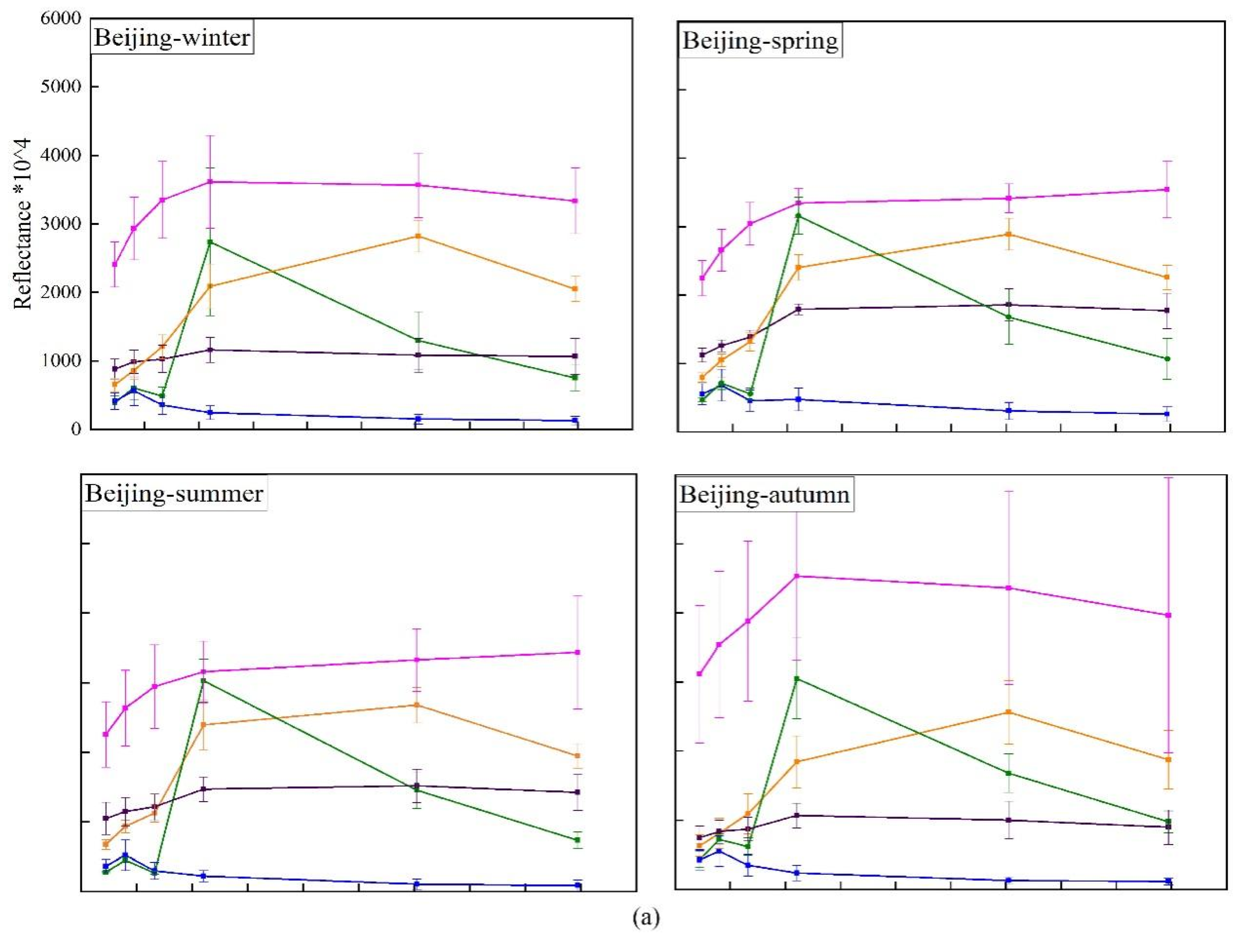
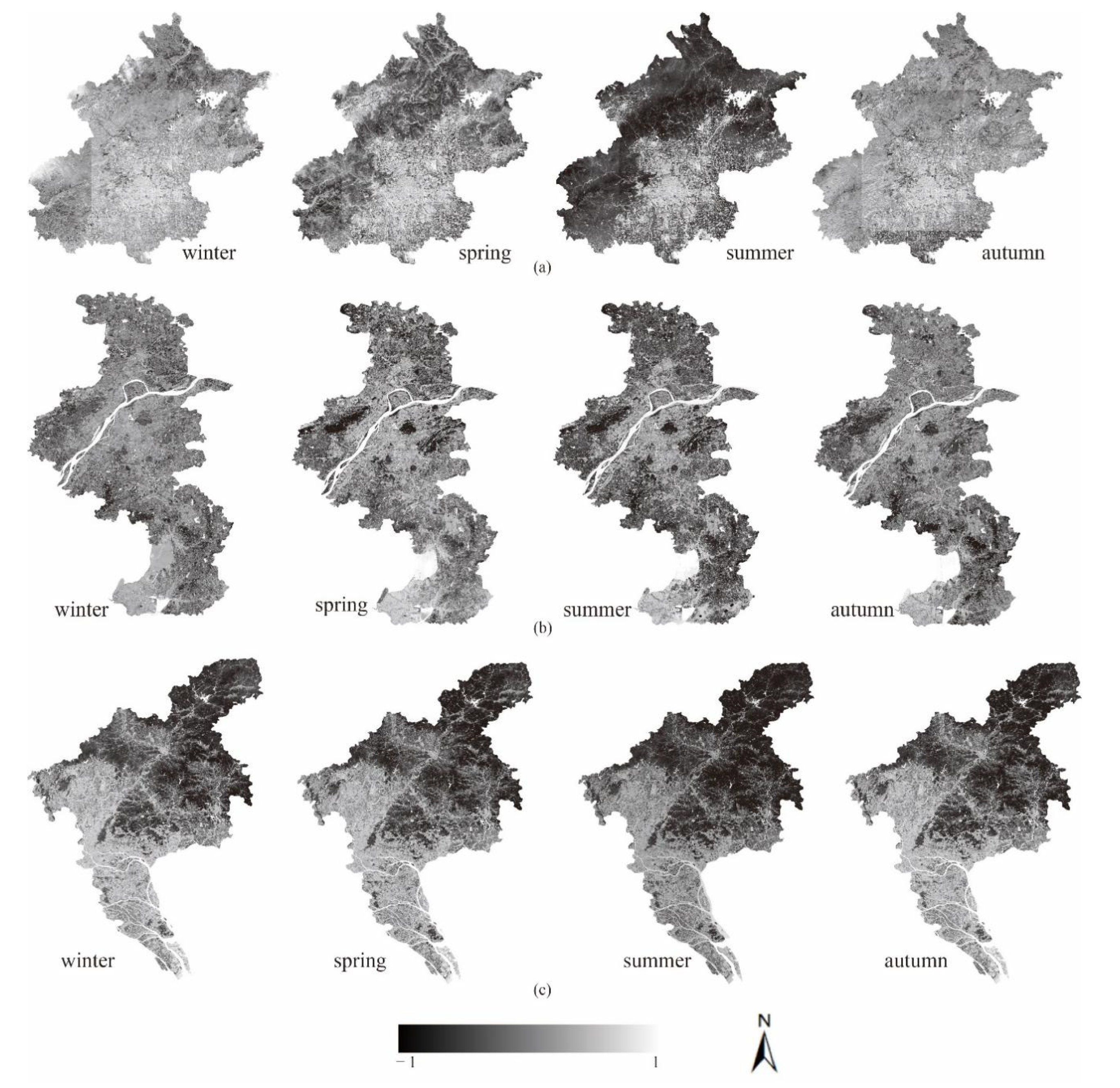
5.1. Influence Relationship between Separation of Bare Soil and Season Selection

In the process of urban impervious surface information extraction, the separation of bare soil from low-albedo impervious surfaces is challenging [1]. In cities, bare soil can be divided into natural bare soil (uncultivated farmland) and artificial bare soil (construction sites). In most cities of China, the reflectance of natural bare soil varies with vegetation cover and season. The relationship can be described as nd2 = nd2_bse^−ad + nd2_dv(1 − e^−ad) [52]. When there is no vegetation, spectral reflectance is entirely provided by natural bare soil. Conversely, when vegetation cover is very dense, there is no contribution from the underlying soil. However, artificial bare soil occupies the main part of the interior of a city. Due to the influence of construction, artificial bare soil surfaces are compacted, so they gain high spectral reflectance and become the main influencing factor for the extraction of impervious surface information.

Reducing the influence of bare soil is the main goal of many researchers. Many studies have shown that the use of time-series remote sensing images can effectively reduce the impact of artificial bare soil for extracting impervious surface information [53,54,55,56]. Therefore, we applied Sentinel-2 MSI images and constructed the NISI by analyzing the characteristics of spectral curves for three different regions across four seasons. However, a small number of artificial bare soil areas were confused with some low-albedo impervious surface areas, though the impaction degree was within an acceptable range (see Table 5, Table 6 and Table 7). Compared to bare soil, the NISI values of vegetation and water were found to be quite different from the NISI values of impervious surfaces and could be well-distinguished from impervious surfaces (see Table 3).

In this article, we selected bare soil and impervious surface pixels in three different regions across four seasons through visual interpretation. The SDI was used to quantitatively characterize the degree of distinction between bare soil and impervious surfaces.

Table 9. The SDI between impervious surfaces and bare soil across four seasons in different areas.

	Winter	Spring	Summer	Autumn
Beijing	1.2022	1.7664	1.8648	1.9601
Nanjing	1.2607	1.8690	1.9928	1.8098
Guangzhou	1.3489	1.1906	1.1468	1.1670

shows that in Northern China, the most suitable periods to distinguish between bare soil and impervious surfaces were spring, summer, and early autumn; meanwhile, in Guangzhou (affected by the rainy season from May to June), the appropriate extraction time was found to be from September to February of the following year.

5.2. Threshold Selection Strategy of NISI

The selection of the threshold is the key to the NISI extraction of impervious surface information because it directly determines the accuracy of NISI detection. However, threshold selection methods sometimes underestimate or overestimate impervious surfaces in urban areas. Due to the differences in spectral reflectance, low thresholds may occur in densely populated city areas and higher thresholds may appear in urban fringe areas with higher spectral reflectance due to more buildings with colored roofs. We adopted a trial-and-error method based on F_pb to dynamically adjust the image thresholds in different regions, effectively reducing the impact of threshold selection.

The developed approach to determine the threshold of the NISI demonstrated some advantages: (1) the threshold determination of this algorithm is flexible and can be adjusted according to different images, avoiding the error of fixed threshold; (2) the optimal threshold solution is ensured through various constraints, thus improving its extraction accuracy [41]; The accuracy of threshold selection also depend on the ability of the proposed NISI to extract different land-cover types. In this study, the NISI was used to transform the original Sentinel-2 MSI images into grayscale images, with enhanced impervious surfaces being grayer. This enhanced discrimination is helpful in improving the threshold using the trial-and-error method based on F_pb. Therefore, the construction of the NISI is a prerequisite for realizing threshold selection. In addition, the determination of the threshold fully considers the response degree of different locations and seasonal index images for various land-cover class. Table 3 shows that the changes in geographic space and seasons could greatly influence the selection of the threshold.

5.3. Validation and Evaluation

Relative accuracy is widely used to evaluate the performance of impervious surface indices, such as RF-based [57,58,59], SVM-based [17,60,61], and CART [62] indices. In this study, these algorithms had high omission errors and misclassifications due to the limited quantity and quality of the self-constructing samples. However, compared to these machine learning algorithms, the PA and UA of impervious surface and bare soil information extraction of the NISI were better (see Table 5, Table 6 and Table 7), which provided a necessary supplement for the quantitative validation of the NISI and enhanced the credibility of accuracy verification. Some samples contained mixed pixels that were easily confused, particularly in areas with complex and heterogeneous land-cover types such as old urban areas and the urban fringe.

This study provides a better solution to map urban impervious surfaces in complex urban environments by combining spectra from world-recognized spectral libraries and the spectra of typical objects in Sentinel-2 MSI images. In addition, our strategy also solves the problem of separation between artificial bare soil and most impervious surfaces in urban areas. Based on freely available Sentinel-2 images and open-access software, our study provides a reproducible workflow that can be used to map impervious surface distributions on an annual basis for large areas and may therefore provide up-to-date information on land-cover management and ecological assessments at local and regional scales.

6. Conclusions

6.1. The Advantages of NISI Model

As a major biophysical component of urban environments, impervious surface abundance and spatial distribution are essential for land-cover studies. Impervious surface indices may serve as a convenient means of extracting impervious surface information from remote sensing imagery. However, the complexity of the impervious surface spectrum—as well as its dependence on the chemical properties and physical composition, structure, color, and surface roughness of impervious materials—make specifying an impervious surface index difficult. To address this issue, the authors of this article proposed an empirical method for establishing the NISI and discussed its separability from other permeable features. The following conclusions were drawn.

(1)

The NISI was generated by using the spectral characteristic of world-recognized spectral libraries and Sentinel-2 MSI images in different areas and seasons. This index improved the identification of impervious and non-impervious surfaces. The NISI can be applied to various remote sensing images at different spectral and spatial resolutions, as the derivation of the NISI does not depend on SWIR and TIR wavebands.

(2)

A comprehensive comparison of other indices and machine learning algorithms ensured the correctness and effectiveness of the NISI model through qualitative and quantitative performance evaluation methods. Overall, compared to other existing methods for extracting urban impervious surface information, the NISI model demonstrated better performance. In this study, we selected three study areas with different latitudes, city clusters, and representations. The NISI as applied to remote sensing images of different spatial resolutions and showed strong generalization.

6.2. Limitations and Feature

Despite the aforementioned advantages, the NISI has limitations. In our study, the study areas we selected are small, so we could not evaluate the use of the NISI in a large-scale (national or even global) area, which is worth further study. Gong et al. [63] and Zhang et al. [64] solved this problem well by using multisource and multitemporal remote sensing datasets to produce a 30 m global impervious surface map, which is worth considering and referencing. In addition, the NISI consists of three visible bands and one NIR band, and the index value was found to be easily affected by the color of ground objects, resulting in the confusion of yellow impervious surfaces (such as yellow roofing) and bare soil. Therefore, the extraction of impervious surface information could be easily underestimation in some urban areas. To reduce these types of overestimation and underestimation errors, we could also add LiDAR information in future research. LiDAR data have been increasingly used in many geospatial applications due to their high resolution, short processing time, and low cost. At the same time, LiDAR data focus solely on the geometry information of ground objects. Therefore, building information can be better extracted and combined with LiDAR data, thus reducing the confusion between yellow roofs and bare soil. In the future, we will also explore the inclusion of the spatial domain of Sentinel-2 data to better identify the urban extent and separate similar land-cover classes.

References

1. Weng, Q. Remote sensing of impervious surfaces in the urban areas: Requirements, methods, and trends. Remote Sens. Environ. 2012, 17, 34–49. [Google Scholar] [CrossRef]
2. Arnold, C.L., Jr.; James Gibbons, C. Impervious Surface Coverage: The Emergence of a Key Environmental Indicator. J. Am. Plan. Assoc. 1996, 62, 243–258. [Google Scholar] [CrossRef]
3. Weng, Q.; Lu, D. A sub-pixel analysis of urbanization effect on land surface temperature and its interplay with impervious surface and vegetation coverage in Indianapolis, United States. Int. J. Appl. Earth Obs. Geoinf. 2008, 10, 68–83. [Google Scholar] [CrossRef]
4. Myint, S.; Brazel, A.; Okin, G.; Buyantuev, A. Combined Effects of Impervious Surface and Vegetation Cover on Air Temperature Variations in a Rapidly Expanding Desert City. Gisci. Remote Sens. 2010, 47, 301–320. [Google Scholar] [CrossRef]
5. Kotarba, A.Z.; Aleksandrowicz, S. Impervious surface detection with nighttime photography from the International Space Station. Remote Sens. Environ. 2016, 176, 295–307. [Google Scholar] [CrossRef]
6. Brun, S.E.; Band, L.E. Simulating runoff behavior in an urbanizing watershed. Comput. Environ. Urban Syst. 2000, 24, 5–22. [Google Scholar] [CrossRef]
7. Zhuo, L.; Shi, Q.; Tao, H.; Zheng, J.; Li, Q. An improved temporal mixture analysis unmixing method for estimating impervious surface area based on MODIS and DMSP-OLS data. ISPRS J. Photogramm. Remote Sens. 2018, 142, 64–77. [Google Scholar] [CrossRef]
8. Lambin, E.F.; Geist, H.J.; Lepers, E. Dynamics of land-use and land-cover change in tropical regions. Annu. Rev. Environ. Resour. 2003, 28, 205–241. [Google Scholar] [CrossRef] [Green Version]
9. Sexton, J.O.; Song, X.P.; Huang, C.; Channan, S.; Baker, M.E.; Townshend, J.R. Urban growth of the Washington, D.C.-Baltimore, MD metropolitan region from 1984 to 2010 by annual, Landsat-based estimates of impervious cover. Remote Sens. Environ. 2013, 129, 42–53. [Google Scholar] [CrossRef]
10. Herold, M.; Roberts, D.A.; Gardner, M.E.; Dennison, P.E. Spectrometry for urban area remote sensing—Development and analysis of a spectral library from 350 to 2400 nm. Remote Sens. Environ. 2004, 91, 304–319. [Google Scholar] [CrossRef]
11. Wu, C. Normalized spectral mixture analysis for monitoring urban composition using ETM + imagery. Remote Sens. Environ. 2004, 93, 480–492. [Google Scholar] [CrossRef]
12. Yang, J.; He, Y. Automated mapping of impervious surfaces in urban and suburban areas: Linear spectral unmixing of high spatial resolution imagery. Int. J. Appl. Earth Obs. Geoinf. 2017, 54, 53–64. [Google Scholar] [CrossRef]
13. Okujeni, A.; van der Linden, S.; Tits, L.; Somers, B.; Hostert, P. Support vector regression and synthetically mixed training data for quantifying urban land cover. Remote Sens. Environ. 2013, 137, 184–197. [Google Scholar] [CrossRef]
14. Ou, J.; Liu, X.; Liu, P.; Liu, X. Evaluation of Luojia 1-01 nighttime light imagery for impervious surface detection: A comparison with NPP-VIIRS nighttime light data. Int. J. Appl. Earth Obs. Geoinf. 2019, 81, 1–12. [Google Scholar] [CrossRef]
15. Okujeni, A.; Canters, F.; Cooper, S.D.; Degerickx, J.; Heiden, U.; Hostert, P.; Priem, F.; Roberts, D.A.; Somers, B.; van der Linden, S. Generalizing machine learning regression models using multi-site spectral libraries for mapping vegetation-impervious-soil fractions across multiple cities. Remote Sens. Environ. 2018, 216, 482–496. [Google Scholar] [CrossRef]
16. Sun, Z. Estimating urban impervious surfaces from Landsat-5 TM imagery using multilayer perceptron neural network and support vector machine. J. Appl. Remote Sens. 2011, 5, 053501. [Google Scholar] [CrossRef]
17. Zhang, L.; Zhang, M.; Yao, Y. Mapping seasonal impervious surface dynamics in Wuhan urban agglomeration, China from 2000 to 2016. Int. J. Appl. Earth Obs. Geoinf. 2018, 70, 51–61. [Google Scholar] [CrossRef]
18. Deng, C.; Wu, C. BCI: A biophysical composition index for remote sensing of urban environments. Remote Sens. Environ. 2012, 127, 247–259. [Google Scholar] [CrossRef]
19. Liu, C.; Shao, Z.; Chen, M.; Luo, H. MNDISI: A multi-source composition index for impervious surface area estimation at the individual city scale. Remote Sens. Lett. 2013, 4, 803–812. [Google Scholar] [CrossRef]
20. Sun, G.; Chen, X.; Jia, X.; Yao, Y.; Wang, Z. Combinational Build-Up Index (CBI) for Effective Impervious Surface Mapping in Urban Areas. IEEE J. Sel. Top. Appl. Earth Obs. Remote Sens. 2016, 9, 2081–2092. [Google Scholar] [CrossRef]
21. Roberts, D.A.; Smith, M.O.; Adams, J.B. Green vegetation, nonphotosynthetic vegetation, and soils in AVIRIS data. Remote Sens. Environ. 1993, 44, 255–269. [Google Scholar] [CrossRef]
22. Weng, Q.; Hu, X.; Liu, H. Estimating impervious surfaces using linear spectral mixture analysis with multitemporal ASTER images. Int. J. Remote Sens. 2009, 30, 4807–4830. [Google Scholar] [CrossRef]
23. Zhao, Y.I.; Xu, J.; Zhong, K.; Wang, Y. Impervious Surface Extraction by Linear Spectral Mixture Analysis with Post-Processing Model. IEEE Access 2020, 8, 128476–128489. [Google Scholar] [CrossRef]
24. Ridd, M.K. Exploring a V-I-S (Vegetation-impervious surface-soil) model for urban ecosystem analysis through remote sensing: Comparative anatomy for citiest. Int. J. Remote Sens. 1995, 16, 2165–2185. [Google Scholar] [CrossRef]
25. Sun, G.; Chen, X.; Ren, J.; Zhang, A.; Jia, X. Stratified spectral mixture analysis of medium resolution imagery for impervious surface mapping. Int. J. Appl. Earth Obs. Geoinf. 2017, 60, 38–48. [Google Scholar] [CrossRef] [Green Version]
26. Qin, Y.; Xiao, X.; Dong, J.; Chen, B.; Liu, F.; Zhang, G.; Zhang, Y.; Wang, J.; Wu, X. Quantifying annual changes in built-up area in complex urban-rural landscapes from analyses of PALSAR and Landsat images. ISPRS J. Photogramm. Remote Sens. 2017, 124, 89–105. [Google Scholar] [CrossRef] [Green Version]
27. Li, W.; Dong, R.; Fu, H.; Wang, J.; Yu, L.; Gong, P. Integrating Google Earth imagery with Landsat data to improve 30-m resolution land cover mapping. Remote Sens. Environ. 2020, 237, 111563. [Google Scholar] [CrossRef]
28. Esch, T.; Himmler, V.; Schorcht, G.; Thiel, M.; Wehrmann, T.; Bachofer, F.; Conrad, C.; Schmidt, M.; Dech, S. Large-area assessment of impervious surface based on integrated analysis of single-date Landsat-7 images and geospatial vector data. Remote Sens. Environ. 2009, 113, 1678–1690. [Google Scholar] [CrossRef]
29. Reschke, J.; Hüttich, C. Continuous field mapping of Mediterranean wetlands using sub-pixel spectral signatures and multi-temporal Landsat data. Int. J. Appl. Earth Obs. Geoinf. 2014, 28, 220–229. [Google Scholar] [CrossRef]
30. Deng, C.; Li, C.; Zhu, Z.; Lin, W.; Xi, L. Evaluating the impacts of atmospheric correction, seasonality, environmental settings, and multi-temporal images on subpixel urban impervious surface area mapping with Landsat data. ISPRS J. Photogramm. Remote Sens. 2017, 133, 89–103. [Google Scholar] [CrossRef]
31. Xu, H. A new index for delineating built-up land features in satellite imagery. Int. J. Remote Sens. 2008, 29, 4269–4276. [Google Scholar] [CrossRef]
32. Zha, Y.; Gao, J.; Ni, S. Use of normalized difference built-up index in automatically mapping urban areas from TM imagery. Int. J. Remote Sens. 2003, 24, 583–594. [Google Scholar] [CrossRef]
33. Xu, H. Analysis of impervious surface and its impact on Urban heat environment using the normalized difference impervious surface index (NDISI). Photogramm. Eng. Remote Sens. 2010, 76, 557–565. [Google Scholar] [CrossRef]
34. Wang, Y.; Li, M. Urban Impervious Surface Automatic Threshold Detection Model Derived from Multitemporal Landsat Images. IEEE Trans. Geosci. Remote Sens. 2022, 60, 1–21. [Google Scholar] [CrossRef]
35. Xu, H.; Wang, M. Remote sensing-based retrieval of ground impervious surfaces. J. Remote Sens. 2016, 20, 1270–1289. [Google Scholar] [CrossRef]
36. Lin, Y.; Zhang, H.; Lin, H.; Gamba, P.E.; Liu, X. Incorporating synthetic aperture radar and optical images to investigate the annual dynamics of anthropogenic impervious surface at large scale. Remote Sens. Environ. 2020, 242, 111757. [Google Scholar] [CrossRef]
37. Carlson, T.N.; Ripley, D.A. On the relation between NDVI, fractional vegetation cover, and leaf area index. Remote Sens. Environ. 1997, 62, 241–252. [Google Scholar] [CrossRef]
38. Jackson, H.; Prince, S.D. Degradation of non-photosynthetic vegetation in a semi-arid rangeland. Remote Sens. 2016, 8, 692. [Google Scholar] [CrossRef] [Green Version]
39. Demetriades-Shah, T.H.; Steven, M.D.; Clark, J.A. High resolution derivative spectra in remote sensing. Remote Sens. Environ. 1990, 33, 55–64. [Google Scholar] [CrossRef]
40. Tsai, F.; Philpot, W. Derivative analysis of hyperspectral data. Remote Sens. Environ. 1998, 66, 41–51. [Google Scholar] [CrossRef]
41. Li, W.; Guo, Q. A New Accuracy Assessment Method for One-Class Remote Sensing Classification. IEEE Trans. Geosci. Remote Sens. 2014, 52, 4621–4632. [Google Scholar] [CrossRef]
42. Zhang, X.; Li, P. Lithological mapping from hyperspectral data by improved use of spectral angle mapper. Int. J. Appl. Earth Obs. Geoinf. 2014, 31, 95–109. [Google Scholar] [CrossRef]
43. Guo, X.; Li, P. Mapping plastic materials in an urban area: Development of the normalized difference plastic index using WorldView-3 superspectral data. ISPRS J. Photogramm. Remote Sens. 2020, 169, 214–226. [Google Scholar] [CrossRef]
44. Nedkov, R. Orthogonal transformation of segmented images from the satellite sentinel-2. C. R. L’Academie Bulgare Des. Sci. 2017, 70, 687–692. [Google Scholar]
45. Radeloff, V.C.; Mladenoff, D.J.; Boyce, M.S. Detecting Jack Pine Budworm Defoliation Using Spectral Mixture Analysis. Remote Sens. Environ. 1999, 69, 156–169. [Google Scholar] [CrossRef]
46. Deng, Y.; Wu, C.; Li, M.; Chen, R. RNDSI: A ratio normalized difference soil index for remote sensing of urban/suburban environments. Int. J. Appl. Earth Obs. Geoinf. 2015, 39, 40–48. [Google Scholar] [CrossRef]
47. Thomas, I.L.; Ching, N.P.; Benning, V.M.; D’Aguanno, J.A. A review of multi-channel indices of class separability. Int. J. Remote Sens. 1987, 8, 331–350. [Google Scholar] [CrossRef]
48. Kailath, T. The Divergence and Bhattacharyya Distance Measures in Signal Selection. IEEE Trans. Commun. Technol. 1967, 15, 52–60. [Google Scholar] [CrossRef]
49. Kaufman, Y.J.; Remer, L.A. Detection of Forests Using Mid-IR Reflectance: An Application for Aerosol Studies. IEEE Trans. Geosci. Remote Sens. 1994, 32, 672–683. [Google Scholar] [CrossRef]
50. Pereira, J.M.C. A comparative evaluation of NOAA/AVHRR vegetation indexes for burned surface detection and mapping. IEEE Trans. Geosci. Remote Sens. 1999, 37 Pt 1, 217–226. [Google Scholar] [CrossRef]
51. Gong, P.; Liang, S.; Carlton, E.J.; Jiang, Q.; Wu, J.; Wang, L.; Remais, J.V. Urbanisation and health in China. Lancet 2012, 379, 843–852. [Google Scholar] [CrossRef]
52. Philpot, W.; Jacquemoud, S.; Tian, J. ND-space: Normalized difference spectral mapping. Remote Sens. Environ. 2021, 264, 112622. [Google Scholar] [CrossRef]
53. Song, X.P.; Sexton, J.O.; Huang, C.; Channan, S.; Townshend, J.R. Characterizing the magnitude, timing and duration of urban growth from time series of Landsat-based estimates of impervious cover. Remote Sens. Environ. 2016, 175, 1–13. [Google Scholar] [CrossRef]
54. Liu, C.; Zhang, Q.; Luo, H.; Qi, S.; Tao, S.; Xu, H.; Yao, Y. An efficient approach to capture continuous impervious surface dynamics using spatial-temporal rules and dense Landsat time series stacks. Remote Sens. Environ. 2019, 229, 114–132. [Google Scholar] [CrossRef]
55. Deng, C.; Zhu, Z. Continuous subpixel monitoring of urban impervious surface using Landsat time series. Remote Sens. Environ. 2020, 238, 110929. [Google Scholar] [CrossRef]
56. Xie, S.; Liu, L.; Zhang, X.; Yang, J. Mapping the annual dynamics of land cover in Beijing from 2001 to 2020 using Landsat dense time series stack. ISPRS J. Photogramm. Remote Sens. 2022, 185, 201–218. [Google Scholar] [CrossRef]
57. Zhang, Y.; Zhang, H.; Lin, H. Improving the impervious surface estimation with combined use of optical and SAR remote sensing images. Remote Sens. Environ. 2014, 141, 155–167. [Google Scholar] [CrossRef]
58. Yoo, C.; Im, J.; Park, S.; Quackenbush, L.J. Estimation of daily maximum and minimum air temperatures in urban landscapes using MODIS time series satellite data. ISPRS J. Photogramm. Remote Sens. 2018, 137, 149–162. [Google Scholar] [CrossRef]
59. Aguirre-Gutiérrez, J.; Rifai, S.; Shenkin, A.; Oliveras, I.; Bentley, L.P.; Svátek, M.; Girardin, C.A.J.; Both, S.; Riutta, T.; Berenguer, E. Pantropical modelling of canopy functional traits using Sentinel-2 remote sensing data. Remote Sens. Environ. 2021, 252, 112122. [Google Scholar] [CrossRef]
60. Angiuli, E.; Trianni, G. Urban mapping in Landsat images based on normalized difference spectral vector. IEEE Geosci. Remote Sens. Lett. 2013, 11, 661–665. [Google Scholar] [CrossRef]
61. Wu, W.; Li, Q.; Zhang, Y.; Du, X.; Wang, H. Two-Step Urban Water Index (TSUWI): A new technique for high-resolution mapping of Urban Surface Water. Remote Sens. 2018, 10, 1704. [Google Scholar] [CrossRef] [Green Version]
62. Leinenkugel, P.; Esch, T.; Kuenzer, C. Settlement detection and impervious surface estimation in the Mekong Delta using optical and SAR remote sensing data. Remote Sens. Environ. 2011, 115, 3007–3019. [Google Scholar] [CrossRef]
63. Gong, P.; Li, X.; Wang, J.; Bai, Y.; Chen, B.; Hu, T.; Liu, X.; Xu, B.; Yang, J.; Zhang, W.; et al. Annual maps of global artificial impervious area (GAIA) between 1985 and 2018. Remote Sens. Environ. 2020, 236, 111510. [Google Scholar] [CrossRef]
64. Zhang, X.; Liu, L.; Wu, C.; Chen, X.; Gao, Y.; Xie, S.; Zhang, B. Development of a global 30m impervious surface map using multisource and multitemporal remote sensing datasets with the Google Earth Engine platform. Earth Syst. Sci. Data 2020, 12, 1625–1648. [Google Scholar] [CrossRef]
Figure 1. (a) The map of China. (b) False-color composite Sentinel-2 image of Beijing. (c) False-color composite Sentinel-2 image of Guangzhou. (d) False-color composite Sentinel-2 image of Nanjing.
Remotesensing 14 03391 g001
Figure 2. (a) Spectral curves of typical ground objects in USGS spectral library. (b) Spectral curves of typical ground objects in the USGS spectral library resampled to the resolution of Sentinel-2 spectra. (c) The spectral reflectance in NIR and visible bands (red, green, and blue) based on the resampled spectral curves of typical ground objects in the USGS spectral library. The blue, green, red, and black dotted lines in Figure 2 indicate the central wavelength of blue, green, red, and NIR bands of Sentinel-2 reflectance spectra, respectively.
Remotesensing 14 03391 g002
Figure 3. Surface reflectance comparison of ground object classes (mean values and standard deviation values) in multitemporal Sentinel-2 images. (ac) Reflectance of the same ground classes covering four seasons in Beijing, Nanjing, and Guangzhou, China, respectively.
Remotesensing 14 03391 g003aRemotesensing 14 03391 g003b
Figure 4. The NISI results based on multitemporal Sentinel-2 MSI images. (ac) NISI gray-scale images in downtown of Beijing, Nanjing, and Guangzhou, respectively. White surfaces are water, high-brightness surfaces are impervious surfaces, and low-brightness surfaces are non-impervious surfaces (vegetation, bare soil and NPV).
Remotesensing 14 03391 g004
Figure 5. Comparison of mixture degree between impervious surfaces and bare soil. Yellow ellipses and red rectangles represent bare soil and impervious surfaces in (ac), respectively. (a) False-color composite Sentinel-2 image of Beijing International airport. (b) True-color composite Sentinel-2 image of Beijing International airport. (c) NISI image of Beijing International airport. (di) Spectral confusion or index-value-overlapping histograms of bare soil and NISI derived from original images, NISI images, and other typical indices images. The horizontal axis is the index value, and the vertical axis is the frequency of index value occurrence in the index images.
Remotesensing 14 03391 g005
Figure 6. The impervious extraction results of different machine learning methods. Row P1 shows Sentinel-2 false-color images. Rows P2–P5 show the results of RF, SVM, CART, and our method (NISI), respectively. (a-1a-4,b-1b-4,c-1c-4) show the results of RF, SVM, CART, and NISI in Nanjing, Beijing, and Guangzhou, respectively. The yellow polygons denote some examples where our method outperformed RF, SVM, and CART. The black polygons denote some examples where RF, SVM, and CART outperformed our method.
Remotesensing 14 03391 g006