Article

Aeronautics Application of Direct-Detection Doppler Wind Lidar: An Adapted Design Based on a Fringe-Imaging Michelson Interferometer as Spectral Analyzer †

Deutsches Zentrum für Luft- und Raumfahrt, Institut für Physik der Atmosphäre, 82234 Oberpfaffenhofen, Germany
*
Author to whom correspondence should be addressed.
This article belongs to the Special Issue Selected Papers of the European Lidar Conference.
Current address: Sill Optics GmbH & Co., KG, 90530 Wendelstein, Germany.
Remote Sens. 2022, 14(14), 3356; https://doi.org/10.3390/rs14143356
Submission received: 23 June 2022 / Revised: 5 July 2022 / Accepted: 8 July 2022 / Published: 12 July 2022
(This article belongs to the Special Issue Selected Papers of the European Lidar Conference)

Abstract

:
We report on the development of a novel direct-detection Doppler wind lidar (DD-DWL) within the strong requirements of an aeronautic feed-forward control application for gust load alleviation (GLA). This DD-DWL is based on fringe imaging of the Doppler-shifted backscatter of ultraviolet laser pulses in a field-widened Michelson interferometer (FW-FIMI) using a fast linear photodetector. The double approach of detailed simulation and demonstrator development is validated by field measurements with reference wind sensing instrumentation. These experiments allow us to establish wind determination precision at a high repeat rate, short range resolution and close distance of approximately 0.5 m/s, which is in accordance with the dedicated simulations. These findings lead us to the conclusion that this FW-FIMI-based Doppler wind lidar is a pertinent development meeting the special requirements of this aeronautics application. Second, the developed simulators are well suited (given their validation) to be used in the overall and full analysis as well as the optimization of the lidar-based GLA control scheme.

1. Introduction

Doppler wind lidars (DWLs) are used throughout the atmospheric science community, particularly for boundary layer studies, and may today be considered state-of-the-art measurement devices. In recent years, wind energy-related research and industrial applications [1] have nurtured the spread of compact and cost-effective coherent DWL systems. Ground-based aeronautics applications, such as aerodrome proximity aviation weather analyses (shear winds, gust fronts, wake vortices), rely on such DWLs as well [2]. For longer range (i.e., reaching beyond the planetary boundary layer), higher-power coherent DWLs or direct-detection (DD) DWLs must be employed (see [3] for instance). Such DD technology is also utilized in the recent spaceborne European (ESA) wind satellite system aboard Aeolus, as well as in its airborne demonstrator A2D (operated by the German Aerospace Center DLR) [4]. The predominant reason for employing notoriously more complex DD lidars from a technical perspective is their ability to deliver wind measurements in aerosol-laden, mixed and pure molecular air, as opposed to coherent DWLs that exclusively rely on the spectrally narrow aerosol backscatter and are thus dependent on a sufficient aerosol content. This condition is often hard to satisfy outside the planetary boundary layer.
The present publication focuses on an airborne application of DWLs in aeronautics, i.e., for gathering direct atmospheric information aboard individual aircraft. Actually, this application has been under discussion since the invention of laser and lidar [5]. In fact, test flights of virtually all generations of coherent DWLs (from CO2 to solid-state and fiber laser technology) and direct-detection DWLs have been undertaken since the early 1970s [6]. The main purpose was and remains the remote detection of turbulence and wake vortices ahead of the aircraft (being invisible to any other instrumentation such as airborne radar) with the goal of taking actions such as avoidance or mitigation. Despite these efforts, and although turbulence is the second major cause (after system or component failure) [7] of enroute accidents in civil aeronautics, with an increasing trend [8], so far, none of such setups have found their way into an application or product. One reason is the objective technical complexity of lidar systems in general. A second reason may be seen, already developing during the early lidar years, in the increased structural resilience of aircraft against the effects of turbulence encounter (due to structural optimizations and strong certification standards), rendering turbulence remote sensing more or less unnecessary.
However, today, multiple predicaments alter the situation: the aeronautics sector of tomorrow faces increased demand for ecologic (besides economic) efficiency and sustainability [9,10,11]. Apart from aviation fuel issues, this ultimately implies more lightweight airframe structures (e.g., including wings with higher aspect ratio). These structures will have to be designed to at least the same turbulence design loads specified by the authorities (CS25.341 [12]). Second, despite the climate crisis, the long-term growing air traffic is expected to “strongly” recover from the dip caused by the COVID-19 pandemic and further increase [9,13]. Meanwhile, for virtually all global greenhouse gas (GHG) emission pathways, climate models project significantly higher turbulence abundance with strong gusts in typical cruise flight altitudes and most employed global routes [14]. Last, with the conceivable introduction of climate-optimized flight routes [15], one should expect a strong competition on “available” ones, with a possibly lower threshold on turbulence-laden ones. These factors, the multiplication of indirectly required augmented airframe vulnerability and increased exposure shall lead to a turning point of the described situation, with investments in advanced sensory and mitigation schemes.
In this context, the DLR has been exploring turbulence mitigation systems for a long time, both on the remote sensing side and on the respective flight control side. Different from previous orientations, regarding mere protection from turbulence [16], as also pursued elsewhere [17,18], DLR is studying next-generation feed-forward flight control systems for strong mitigation of atmospheric effects such as turbulence, gusts and wake vortices. In contrast to state-of-the-art feedback control schemes, such feed-forward methods are based on ahead wind information, ultimately to be delivered by a Doppler lidar system [19,20]. What has in the past (at DLR or in general) been hampering the advancement of such schemes was the high demand on a DWL system for delivering wind data with sufficient spatial and temporal resolution and quality.
Now, DLR’s advanced generation of these control schemes may handle partial or comparatively low data yield (i.e., more realistic in terms of lidar delivery) due to the use of quasi a priori information on the phenomenon to be encountered. Based on lidar wind measurements (notably in line-of-sight (LOS) projection, with several viewing directions), dedicated algorithms reconstruct the physical wind field in real time from arbitrary free-form or deterministic analytical models; they apply advanced optimization techniques within maximum-likelihood estimations [19,21,22] in order to fit a wind field model to the measurements. The downstream feedforward controller then employs wavelet-based time-frequency decomposition and delivers this information to a command-generation module. This produces commands to individual airframe control surfaces such as rudders or lift devices (spoilers/flaps). As examples, in the simple case of an ahead upward vertical gust, this would be countered by a subtle nose-down maneuver by the tailplane elevators, or for an imminent wake vortex encounter by the initiation of an adverse roll rate, both only tenths of seconds before encounter. Assuming that such a lidar/controller system reliably and categorically mitigates such spurious atmospheric flows and thereby the associated structural loads (e.g., on the wing root), and assuming further that such a system attains certification by civil aviation authorities (an important aspect), this will allow the aircraft manufacturer to reduce structural mass. The resulting mass savings directly translate into fuel consumption (and potentially GHG emission offsetting) cost savings, and in turn into operation cost reduction for client carrier companies. Apart from the direct cost savings due to prevented accidents (in former market assessments [23] considered as the only asset), the savings due to increased efficiency make such a remote sensing system an attractive option to be considered.
The above-described combined model-and-measurement-based determined wind field, given within the relevant spatial frequencies of an aircraft, dramatically decreases the requirements on DWLs for delivery of these wind data, compared to the simple case of feeding only the pure, noisy measurement data to such a controller. Thus, the requirements on DWLs are pushed into technically satisfiable bounds.
DLR studies the interconnection of reducible loads, airframe control and aerodynamics and lidar sensory capabilities in a holistic approach. Thus, a four-part iterative simulation suite [20,24,25] covers the whole chain: lidar performance is modeled both in a simplified analytical and a more physical end-to-end implementation-based simulation, as a function of basic design parameters (see Section 2). A module designated to the wind reconstruction algorithm (WRA) allows the optimization of the LOS wind acquisition with respect to the relevant aircraft frequency responses [26,27]. Different aircraft aeroelastic models (such as the Common Research Model (CRM), initially by NASA) may be used at different flight points (mass, Ma-number, etc.) in order to generate a descriptive aero-elastic state space model of reduced order. This allows the derivation of mechanical loads based on turbulence input [25], where the latter may be discrete gusts or continuous turbulence as defined in the regulatory framework documents [12]. Another block within the simulation ensemble is the feedforward gust load alleviation (GLA) controller itself, with the controller design based on a new multi-channel structured discrete time H formulation [28]. Within the iterative simulation, it may be compared to the load control performance of a basic (feedback) controller.
With this suite of models [29], an iterative analysis is performed for identifying a reasonable set of requirements not only but particularly on the lidar parameters (with receiver, laser and scan/beam director system), all based on a reasonable and useful level of load alleviation (it is noteworthy that due to other aerodynamic loads, such as maneuver-induced loads, a full-scale load reduction is neither necessary nor expedient) and other, possibly competing requirements (such as passenger comfort or other structural loads increase). In other words, over-specification of any sub-component of the whole chain, and in particular, the development- and cost-intensive lidar hardware, is thus avoided.
Consequently, at the present state of development and given the wide field of aircraft and mission profiles, there is not a stringent fixed set of requirements, but rather a parameter space toward a suitable DWL system:
  • Updated rate of the LOS wind measurements from 10 Hz to 20 Hz over the full field (i.e., over several viewing directions, e.g., within a cone);
  • Wind speed precision of around or less 1 m/s in cone-like or screen-like scanning or multiple direction setups;
  • Spatial resolution from 10 m to 30 m, depending on the aircraft mass, wingspan and flight speed (and thus its frequency response to turbulence);
  • Distance ranges of 50 m to 350 m ahead of the aircraft;
and additionally:
  • Consideration of eye safety issues; and
  • Full and provable availability of sufficient functionality in cruise flight conditions.
The latter requirement quite categorically excludes the usage of the coherent DWL technology option due to their dependence on aerosol backscatter (i.e., the related narrow spectral shape needed for an effective frequency estimation). A GLA control system combined with respective airframe structural adaptations for weight savings as described above will have to run through regulatory certification (by civil aviation authorities). There, it will have to be positively proven that sufficient backscatter is virtually always (or in all relevant flight conditions) present for the system’s availability; such evidence may simply not be produced, not even with repeated demonstration of functionality (as in [30] or [31]). In relevant studies with industrial partners (i.e., major airframe OEMs-in our case European ones), it remained a consensus that DD-DWLs are mandatory for a GLA application for airframe weight reduction. Furthermore, in order to optimize the yield in terms of molecular backscatter, short laser wavelengths, such as ultraviolet (UV) ones, are to be preferred. Comparing the figure of merits (e.g., see Table 1 in [16]) of the fourfold combination laser, frequency conversion, molecular backscatter efficiency (scaling with λ4) and detector quantum efficiency, UV even beats green radiation with a factor of about four (for a given fundamental laser system) in efficacy. For these reasons, the legacy AWIATOR [32,33] system had been an ultra-violet (UV) laser-based direct-detection DWL. Thus, the DLR lidar developments started (in 2014) from this premise, too.
Within this publication, the two above-mentioned lidar simulations are reported and validated with a demonstrator. Regarding the latter, a synopsis of design, fabrication and testing in natural wind is presented. All other mentioned aspects are covered in the given references or will be published in respective research domain publications.
Therefore, the document is structured as follows: The following Section 2.1 first treats a simplified analytical model of a Doppler wind lidar to be used in above-described comprehensive load simulation, followed in Section 2.2 by an outline of a specialized physics-based simulator. Then, in Section 2.3, the currently implemented DWL demonstrator is described, based on some design requirement constraints and design choices.
The central part (Section 3) then provides results of actual wind measurements and a performance analysis based on the simulations. The last part (Section 4) concludes and gives the currently and future followed routes for further development.

2. Methods for Validating the Applicability of Direct-Detection Doppler Wind Lidar as Aeronautics Gust Load Alleviation Sensor System

2.1. Analytical Model of a Direct-Detection Doppler Wind Lidar

The lidar simulation model to be used in the overall four-part iterative wind to load control simulation suite constitutes a set of simple analytical equations and a number of carefully chosen and validated system variables. It delivers the wind speed measurement noise level, i.e., the statistical distribution of individual measurements. This distribution, quantified by the variance σ v L O S 2 of wind speed measurements, is the key gauge of the lidar performance. The distribution is derived from the spectral discrimination performance of a non-specific “spectral analyzer”, which is thus applicable to any device determining a spectrum of Gaussian shape by means of analyzing spectral channels. A Doppler wind lidar may thus be considered as a spectral analyzer that estimates the spectral shape (and thus phase, shifted by the wind’s Doppler effect) of (between, respectively) the transmitted and backscattered radiation.
For an “ideal” spectral analyzer (ISA), the statistical distribution of this estimate of frequency shift may be quantified by the Cramér–Rao lower bound (CRLB) of such an estimation [34,35]:
σ v L O S , I S A = σ ν R a y N e
where σ ν R a y is the width of the Rayleigh spectrum (neglecting departure from Gaussian by Brillouin, etc., and given in m/s) at the 1/e1/2 point.
It is given by σ ν R a y = k B · T a i r · N A m a i r , where k B represents the Boltzmann constant, T a i r is the prevailing air temperature, N A is the Avogadro constant (number of molecules per mol), m a i r is the molecular mass of air and N e is the number of photoelectrons generated on the analyzing detector (to be determined later on).
For realistic physical spectral analyzers (not disposing of an infinite number of analyzing spectral channels among other things), such as interferometers with realistic detectors, a correction factor κ C R B realSA must be applied (see below). There are a number of possible technical implementations, stemming from different interferometer types and setups, such as the use of Fabry–Pérot interferometers in imaging setups. Examples in the aeronautics domain are the already-demonstrated AWIATOR system [32,33] with imaging of the circular fringe pattern, the double-edge setup [36], dual- or quadri-channel Mach–Zehnder setups [35] or double-channel Michelson [37] setups and others. The different setups display diverse correction (or penalty) factors and even more different advantages and disadvantages, both depending on application and requirements.
The derivation of the individual CRLB, including the appropriate correction factor κ C R B realSA , is subject to rigorous mathematical treatment. The numerical value is also a function of the prevailing conditions (atmosphere: spectral bandwidth, aerosol backscatter ratio) and spectrometer-related variables (such as phase sensitivity, global contrast and instrument contrast), the latter parameters carefully being optimized to the former. In Table 1, we give examples of the respective penalty factors κ C R B realSA = σ v L O S , realSA σ v L O S , I S A that have been derived in diverse publications. They are given for comparable conditions (atmospheric temperature T a i r = 273 K and backscatter ratio R b = 1 ) relevant for this application.
As we see, the range of penalty factors is relatively narrow; thus, we assumed a fixed semi-optimum value of κ C R B realSA , Sim = 2.3 for the simulations. Furthermore, as we detail in Section 2.3, this value is applicable for the implementation projected and studied by DLR.
Moreover, the real technical implementation admittedly seldom achieves the theoretically prognosed performances, due to technical noise issues, trade-offs, unavoidable degradations, etc. Therefore, we must introduce a further performance-degrading factor that we denote as “technology implementation factor” (TIF). An a priori value for this would be speculative, as it must be determined in calibrated experiments; as we show in Section 2.3, the DLR demonstrator implementation (not optimized, only for demonstration) yields a factor of κ T I F realSA = 1.7.
For the photon noise limited case, or, more correctly, the photoelectron limited case, Equation (1) may thus be given as a function of the lidar system’s signal-to-noise ratio (SNR) where the signal photoelectrons are “available” for the spectrum discrimination:
σ v L O S , r e a l S A , a v = σ ν R a y · κ C R B realSA · κ T I F realSA S N R a v
where S N R a v denominates the synthetic signal-to-noise-ratio obtained by some form of averaging (see below).
The next step consists of the derivation of this signal-to-noise-ratio due to the backscattered photons collected and conditioned by the lidar optics, and impinging on the detector. By using the textbook “lidar-equation” [44], we determine the signal-to-noise ratio of a single observed laser pulse S N R s s :
S N R s s = ρ d e t · η o p t · c · β a t m h , λ · τ a t m h , λ , R · E p · A R x 4 · e · B · R 2
where ρ d e t signifies the detector’s quantum efficiency for the conversion of photons into electrons; η o p t is the optical efficiency of the lidar system (mainly receiving part); c is the speed of light; β a t m and τ a t m are the atmospheric backscatter and transmission, respectively, depending on the altitude h, the wavelength λ of the used laser and the traversed range R up to the target distance ( τ a t m may, however, be neglected to unity for the short distances we consider for the GLA case); E p is the power of a single emitted laser pulse and A R x is the lidar receiving aperture; e is the electron charge; and B is the system’s relevant electronic bandwidth.
Equation (3) may be expanded to the synthetic S N R a v (where the subscript stands for averaged) when averaging a number of pulses N m e a s . It is assumed (and in practice, well proven [16]) that the noise processes of subsequent pulses are uncorrelated, thus Poissonian. Therefore:
S N R a v = S N R s s · N m e a s
with   N m e a s = P R F r refresh
where N m e a s denotes the number of laser pulses aggregated to a synthetic signal. This may be realized in post-processing (digitally), as shown in Section 2.3, but also directly within the detector (analog accumulation), as in past and present airborne (AWIATOR [32,33]) and spaceborne (AEOLUS [45]) direct-detection UV wind lidars. P R F is the laser pulse repetition frequency (or pulse rate) of the pulsed laser and r refresh is the required refresh rate, i.e., the rate at which the wind measurements are collected by the wind estimation algorithm.
An important point in the design is the optimization of the detection system bandwidth to the aimed spatial extent, which is often termed range gate (length) Δ R :
B = c 4 · Δ R
Last, we introduce the power aperture product (P.A.P.), a measure for sizing lidar systems. It represents the trade-off between realistic and affordable laser power P T x = E p · P R F , as well as reasonable and also affordable receiver telescope size A R x (e.g., due to aircraft integration constraints), both being equivalent in the lidar equation:
P . A . P . = P T x · A R x = E p · P R F · A R x
P . A . P . may lead to reasonable estimates on the other important, more engineering-technical design quantity S.W.a.P. (size, weight and electrical power) of the lidar system (laser and receiver systems).
We now combine Equation (2) with Equation (3) through Equation (7) and obtain the above-stated variance of the LOS wind speed determination:
σ v L O S , a v 2 = κ realSA · κ T I F 2 · e η o p t · ρ d e t · k B · T a i r h · N A m a i r · β a t m h , λ · R 2 · r r e f r e s h P . A . P . · Δ R
For detailed analysis and design, this expression can be separated into three distinct terms:
  • The first term represents the Doppler wind lidar technical optics architecture and implementation and remains constant for given (typical) lidar performance values.
  • The second term, the atmospheric contribution, is constant for a given flight altitude h (thus mission profile). Since for realistic (and worst case) estimations, a pure molecular atmosphere should be considered, the backscatter coefficient β a t m collapses into a mere function of the atmospheric temperature T that in turn may be determined by a certain model atmosphere.
  • The third term contains the lidar system design variables; these should be adopted to meet the requirements of the wind reconstruction algorithm to retrieve the LOS wind speed with a certain precision.
This analytic model of such a Doppler wind direct-detection lidar may be used as a simple reference for validating real-world validation measurements, as shown in Section 2.3, as well as for preliminary design studies. A simple numerical exercise shows, for instance:
  • For a decent overall optical efficiency η o p t of about 25%, together with a good detector quantum efficiency (giving a responsivity of 0.12 A/W for the photomultiplier tube (PMT) as used in our demonstrator), the first factor is around 7 · 10 9   kg   m 2   s 2 .
  • The atmospheric term amounts to a value around 1.5 · 10 5   m 3   s 2 for an altitude of 10,000 m and considering a UV wavelength of 355 nm.
  • Together, these factors amount to around 10 3   kg   m 5   s 4 that must be accommodated by the third factor to achieve a wind speed distribution σ v L O S on the 1   m   s 1 level.
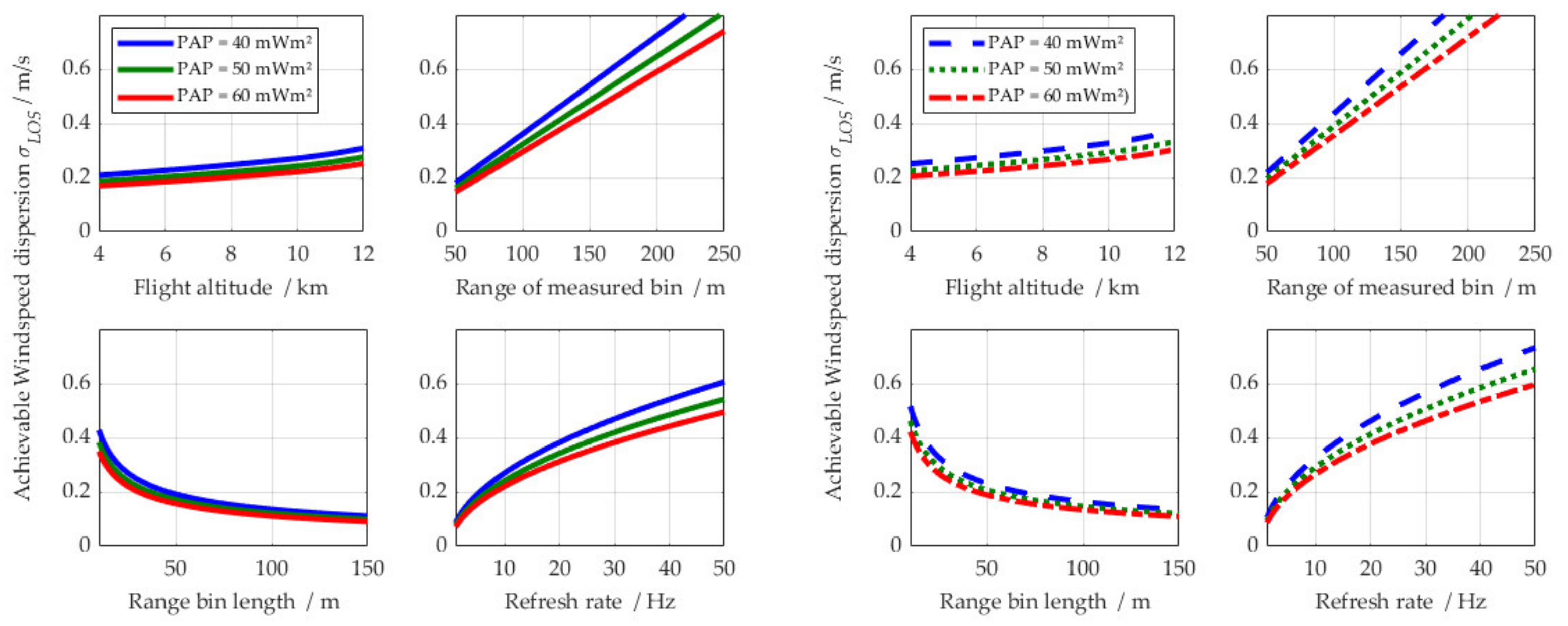
  • Taking as an example, and for ease of calculation, 10 Hz for r refresh , 10 m for the resolution Δ R and 100 m for the considered detection distance R , it may be deduced that a P . A . P . of around 50 mWm² would deliver good wind estimation results of around 0.5 m/s dispersion. Such a P . A . P . may be achieved with a 5 W laser and an effective receiver aperture diameter of 11 cm. Note that the actual laser pulse repetition frequency (PRF) is not a subject here. However, when going into more technical detail, it should be analyzed in detail since too high as well as too low pulse energies may be detrimental for the outcome, either due to overexposing the detector on very short distances, or due to too high noise per pulse, inhibiting a good averaging even with high pulse numbers N m e a s .
Such an exercise is a good starting point for any study of a direct-detection Doppler wind lidar system for whatever application, but here, in particular, for the close-range, more or less horizontal measurement. The following graphs illustrate the respective dependencies, here for default values of R = 75   m , Δ R = 25   m , r refresh = 10   Hz and h = 10 , 000   m and some values for η o p t and P . A . P . that seem realistic to attain in a thoroughly designed system (notably different from our demonstrator in Section 2.3).
It should be noted that, at least for the here-shown fringe-imaging detection approach based on a photomultiplier array (anticipating Section 2.3), an additional analytic accounting of the electronics noise does not strongly modify the outcome of Equation (8). This is illustrated in Figure 1 (right panels, dotted graphs). The main contribution actually stems from the noise figure of the used photomultiplier tube(s). A more rigorous inclusion of actual noise processes may only be achieved by the use of stochastic models, as addressed in the following.

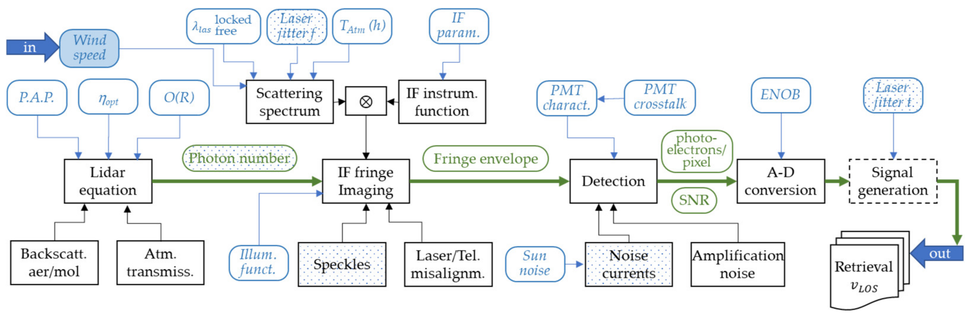
2.2. Physics-Based End-to-End Simulator

In the detailed design process, a more comprehensive simulation should be used that also accounts for additional, real-world physical phenomena. Hence, the above-explained analytical model may be seen as the basis of a somewhat more comprehensive “end-to-end” lidar model of one specific implementation of a direct-detection Doppler wind lidar (DD-DWL) demonstrator (Section 2.3), realized and continuously augmented at DLR [43,46]. Due to the incorporation of the actual technical design, it necessarily loses its generality.
Despite not (yet) including all physics (such as photon paths, turbulent atmospheric optics effects, optical aberrations), it notably contains a statistical means (Monte-Carlo-like) for the simulation of different noise processes (e.g., electronics, optical speckles) and physics of the optical Doppler spectral analyzer. It notably allows, by generation of synthetic digital “measurement” signals, employing the same wind determination algorithm (i.e., the fitting and Doppler phase determination scheme) that is employed for the real lidar demonstrator detailed in Section 2.3. This also allows an optimization of these algorithms by using synthetic measurement data.
Due to modules requiring random number generation (for reproducing random processes such as electronics shot noise, random laser frequency jumps, indicated in Figure 2 as dotted boxes), the whole scheme is executed a high number of times, and the actual quantity σ v L O S , a v of Equation (8) is determined by the standard deviation of realizations. Owing to this repeat magnitude, the end-to-end model is computationally demanding and is hence not suitable to be used directly in the full aircraft simulation mentioned in the introduction. This is the reason why the analytical model of Equation (8) must be used in the overall aircraft GLA simulation procedure.
Given its extent, we do not fully describe this model here (more thoroughly in [46]), but briefly touch upon it: referring to Figure 2, the basis of this model is again the lidar equation that delivers, for each laser pulse, the photon number (over time) collected by the optics as a function of the receiver variables, including the overlap function O R . The next module derives the spatial distribution of the actual fringe produced by our Michelson interferometer as a convolution of the atmospheric scattering spectrum and the interferometer instrument function. The former (as above Equation (1)) also includes a random laser frequency fluctuation; the latter is a function of the interferometer (IF) design parameters, incorporating optics defects by a change in the IF’s contrast function. A separate module overlays the spatial distribution (intensity/photon number fluctuation) due to atmospheric and fiber-induced (as part of the receiver system) speckles onto the determined fringe intensity distribution function. This intensity envelope (over space and time) is then handed over to a detector module that represents the used photomultiplier array with its characteristics (gain, blind zones, crosstalk between channels, etc.). With the time response of detector and amplifier, it also affects the temporal distribution of the single lidar “pulse” form. The related noise currents (function of detector and amplifier characteristics) are again modeled by a random number approach. For each realization, the resulting photoelectron number is then given to the digital sampling unit and converted to bits, as in the real system, respecting the effective number of bits (ENOB). It also takes account of the pulse-to-pulse temporal jitter (in reference to the overall clock) inherent to our laser system. Then, (still quite idealized) measurements are at hand for evaluation by the fringe fit routine (Section 2.3).

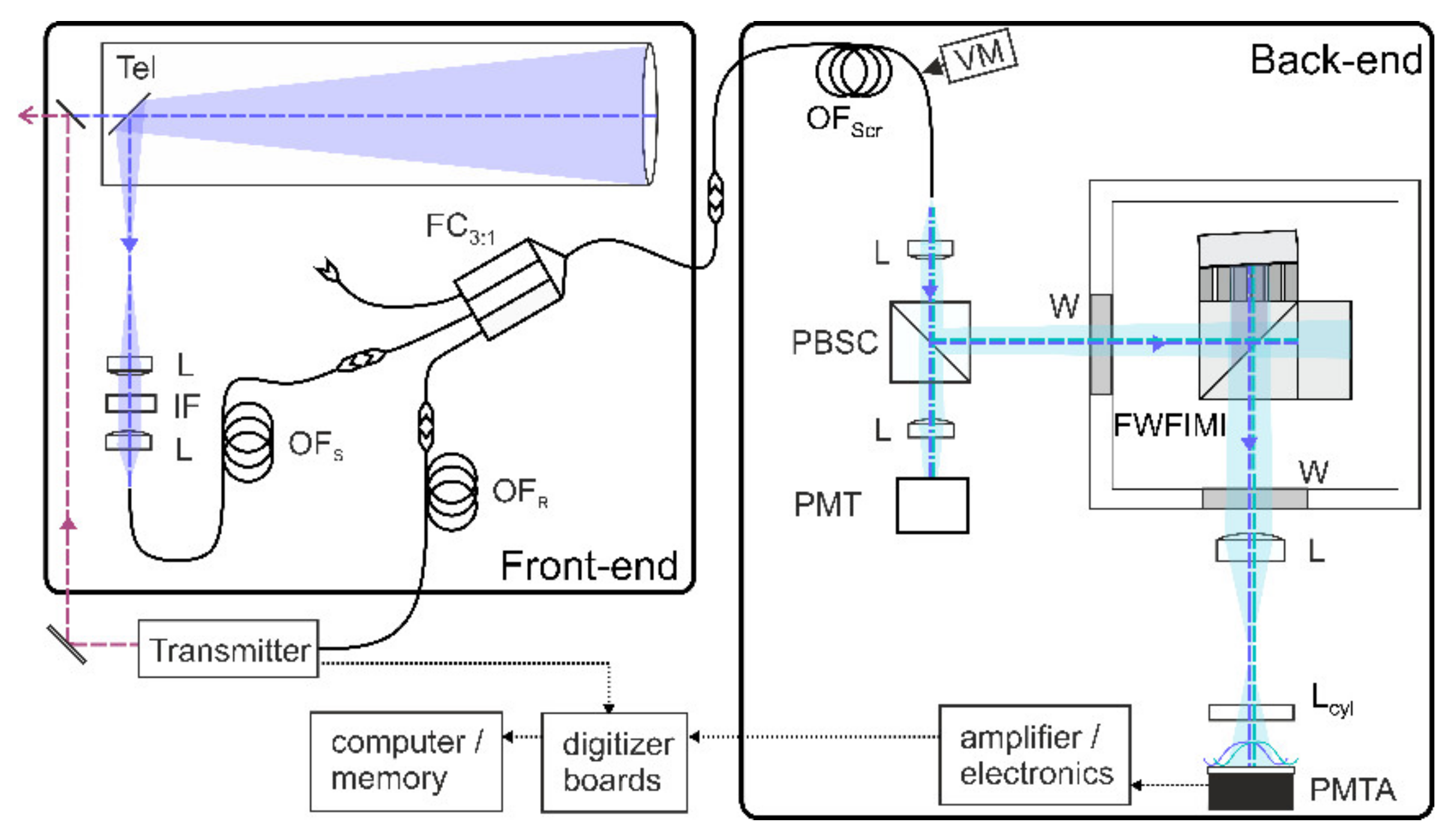
2.3. Demonstrator of the DD-DWL for Gust Load Alleviation (GLA) Application

As addressed in the introduction, DLR developed a functional demonstrator of a DD-DWL adapted to the special set of requirements dictated by the application of feed-forward GLA control. This aeronautics lidar prototype (termed AEROLI) serves as proof for both the ongoing optimization simulation series (regarding specifications) and for the technical learning and optimization in terms of implementation. For several reasons (as discussed below), we implemented a special Michelson interferometer as the spectral analyzer, i.e., transforming the spectral information of the emitted laser pulse (the reference) and the backscattered (the atmospheric Doppler-shifted signal) into spatial information that is observable by a detector. The design of this part of the Doppler lidar is thoroughly addressed in [43]; thus, here, we recall only the basic functionalities.

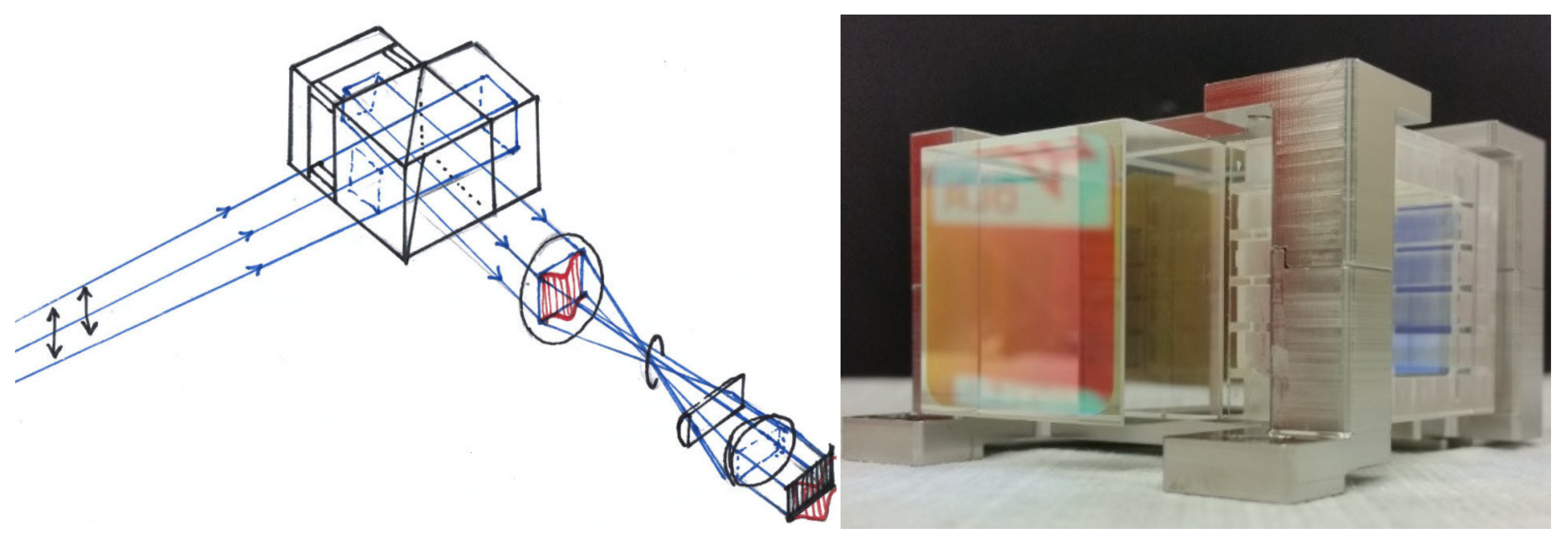
2.3.1. The Spectral Analyzing Part: FW-FIMI

The needed close measurement range (<300 m, farther away would not make sense due to the inherent unstable property of turbulence) infers a maximized overlap within this region and thus a large field of view (FOV) of several milli-radians. For aircraft-compatible telescope sizes (and even more for bigger apertures) and feasible optics dimensions of the spectral analyzer, the resulting magnification translates this FOV to important angular distributions. Therefore, an interferometer for this application must be field-widened (i.e., with near-invariant response to this angular range) to avoid significant loss of contrast. This field widening (FW) may be realized with two-path interferometers such as Mach–Zehnder (MZ) and Michelson (MI) setups, as opposed to multiple-path interferometers such as Fizeau and Fabry–Perot. The MZ technique has, for example, been adopted by French LATMOS [47] in their multi-purpose lidar LNG and by Ball Aerospace in the different generations of the OAWL lidar [48,49].
For our application, we opted for a field-widened Michelson interferometer (see Figure 3) for fringe imaging (FW-FIMI) for several reasons, inter alia, the novelty of development. Fringe imaging notably allows the measurement to be independent (invariant) of the spectral shape of the atmospheric backscatter, which is determined by the ratio of aerosol to molecular backscatter and temperature. Once a fringe is produced, the mere comparison of the barycenters of reference to signal fringes gives the Doppler shift. The field widening is achieved by implementing the two interferometer arms with highly different indices of refraction. In our implementation, this is achieved with one glass and one air arm, where the latter may be used to fine-tune the IF (by air temperature) to the spectral operation point.
Furthermore, a FIMI may be implemented with a slightly slanted mirror (some µrad), producing a linear fringe pattern (instead of circular), which may easily be imaged on a linear detector array (instead of a two-dimensional array as used, e.g., in AWIATOR [32,33]). This grants optimum photon efficiency due to high SNR on each of the few detector elements (pixels).
An airborne application calls for resilience towards vibrations and temperature variations, what may be responded to by a monolithic interferometer architecture, comparatively easily achieved with an MI. Such a monolithic FW-FIMI can be constructed to be both field widened (FW-FIMI) and temperature compensated. This monolithic setup is obtained by molecular adhesion of the different elements, the beamsplitter cube’s triangular cylinders, the glass arm, the air arm’s mirror and the air arm’s spacers. The latter are stacked composites of fused silica and calcium fluoride for an optimization of the resulting coefficient of thermal expansion. Last, our FW design is arranged (with respect to field widening) so that the whole interferometer may be tilted to the incident light (by roughly 2°), enabling two-channel operation (transmit and reflected channels).
Our previous publication [43] detailed the respective design optimization in terms of the choice of the free spectral range (FSR) of 10.7 GHz (with an optical path difference OPD of 28 mm) for the optimized value of κ C R B realSA = 4.4 , as in Table 1 (last line), for single-channel operation. As Figure 4 illustrates, this is a compromise. For higher FSR, the fringe phase sensitivity with respect to the Doppler shift decreases. For smaller FSR, the global fringe contrast becomes too small for an efficient determination of the fringe phase. Figure 4 also shows the dependence on the fringe visibility V (instrumental fringe contrast), another constituent of the global fringe contrast. This instrumental contrast term V accounts for many real-world drawbacks, such as the illumination with a spatially and angularly extended source, the imaging error of the fringe localization plane, the effective beamsplitter ratio, the interferometer illumination and the discrete number of detector pixels illuminated by the IF’s fringe. This aspect is addressed in detail in appendix C.6 of [38]. We could budget these factors to a cumulative value of V t h e o 98 % . Experimentally, we could prove that V e x p 95 % in a detailed fringe characterization setup (Chapter 3.5.2 of [38]). Here, we used a frequency-tuned continuous-wave 355 nm laser and a CCD camera for fringe analysis. We attribute the small discrepancy to this characterization setup (imaging and camera), so we are confident that the V-factor decrease is nearly negligible in our instrument. Regarding the other design criteria, such as the field widening, the mirror skew, the temperature compensation and fabrication tolerances, our previous publication [43] also took numerical account of these.
Figure 3 illustrates the actual illumination setup of the FW-FIMI. A collimated beam of s-polarized light produces one period of the cosine-like fringe pattern at the interferometer output. This pattern is then imaged onto the linear detector in the following way: A cylinder lens compresses the two-dimensional intensity fringe pattern along the vertical axis, while a collecting lens images the fringe localization plane onto the detector plane.
As a detector, we use a 32-element photomultiplier tube array (PMTA), and only 16 pixels are illuminated. The signal current of each element of the PMTA is converted to a voltage by an equal set of transimpedance amplifiers (TIA) and is then digitized by two eight-channel analog-to-digital converter boards (Section 2.3.4). The use of such a fast PMT detector allows for the production of a continuous, “real” lidar backscatter signal, other than, e.g., in AWIATOR [32,33], where only a single distance measurement was available. These several range bins of measurements permit the wind reconstruction algorithm (see Introduction) of the control scheme to dispose of substantially more data (even though less precise for farther ranges), which is beneficial for the wind field estimation. In the here-reported version of the experiment, the TIA admittedly had to be tuned to a rather slow bandwidth (resulting in temporally stretched electronic pulses) in order to avoid aliasing problems on the short laser reference pulse (see Section 2.3.3) that features a certain temporal jitter with respect to the overall (and thus also digitizer) clock.
As depicted in Figure 5, the interferometer (FWFIMI) is housed in a thermally controlled airtight housing. The interferometer is illuminated by a collimated beam issued from a square-core fiber (Section 2.3.2) that by lens L actually forms an image of the fiber-tip near field onto the IF’s fringe localization plane.
A present disadvantage is the mandatory use of s-polarized light due to the poor splitting ratio (strongly deviating from 50:50) in p-polarization that would translate into a strong contrast reduction. So far, for our demonstration purposes, we operate the lidar with s-polarization only (selected by a polarizing beam splitter cube, PBSC in Figure 5), accepting the loss of 50% of the signal. However, we use this signal for another PMT detector for practical purposes within experimentation activities.

2.3.2. Receiver Front-End: Light Collection and Fiber Architecture

The field-widening aspect of the IF allows for an additional feature within our implementation: We use large-core multi-mode optical fibers (OFs) for the transport of the backscattered optical flux from telescope collection to the interferometer for several reasons. First, using OFs eases the construction and implementation of such lidar systems, eventually for the operation within the confined space of an aircraft. Beyond that, they also allow for easy combination, splitting, etc., via typical fiber modules such as couplers. In this context, we use a fiber coupler to combine the reference laser light (coming directly from the laser via fiber) with the atmospheric signal.
Most importantly, large-core OFs provide scrambling [50,51], i.e., annihilating of angular information, thus (at least theoretically) overcoming the need for range-resolved calibration.
Moreover, OFs allow for shaping the optical flux to nearly arbitrary shapes (such as rectangular top hat) better suited for detector illumination than “natural” circular Gaussian ones.
Lastly, OFs produce speckles themselves, but when using a large core with a very fine speckle pattern (due to the high diversity within the fiber). This facilitates the spatial averaging of atmospheric (molecular and aerosol backscatter-generated) speckles that generate far coarser speckle patterns (in particular, aerosol backscatter). This aspect is also addressed in detail in [38,43].
In our setup, we thus implemented a fiber architecture based on 600 µm diameter cores. After collection of the backscattered light by the telescope (cf. Figure 5), intermediate collimation for transmission through a narrow interference filter (IF), this light is injected in a 600 µm standard circular-core fiber. This telescope (with 140 mm aperture) and injection setup is based on the hardware of a previous airborne backscatter lidar [16], used in the European Commission 7th framework project DELICAT. The aforementioned fiber is then connected to a custom-built 3:1 fiber coupler, allowing the combination with the reference laser light and also other sources such as LED for experimentation. In some versions of our experiments, the laser light is also retarded by a fibered delay line in order to arrange the reference laser pulses temporally after (spatially behind) the atmospheric signal.
Then, the circular fiber is connected to a dedicated 600 µm square-core scrambling fiber (OFScr) that may also be attached to a vibration device for temporal speckle averaging. In sum, we may say that the combined effort of large-core fibers and the one-dimensional compression of the fringe image reduces the speckle noise contribution in a very satisfactory way.

2.3.3. Laser Transmitter

The laser transmitter used for these experiments is by no means optimized or specifically adapted to the currently targeted application, but it serves the purpose well. The WALES/DELICAT system has been reported in previous publications ([16,52]). This high-power (8 W in UV 355 nm), low-pulse-rate (100 Hz) laser is of the master oscillator power amplifier (MOPA) architecture.
The MO is notably a diode-pumped single-crystal Nd:YAG nonplanar ring oscillator (NPRO) running intrinsically single-mode. This NPRO allows us to tune the laser’s frequency over 3.5 GHz (in the fundamental IR wavelength), thus covering the whole FSR of the interferometer in the UV. This is an important asset to scan the illumination function of the spectral analyzer part of the receiver, which—so far—proved more satisfactory than a white light approach based on an LED. A drawback of this NPRO architecture is the passive Q-switching mode that engenders a certain (yet small) temporal jitter of 0.5 µs (at 1 σ). This leads to aliasing-like problems when sampling short electronic pulse forms produced by the very short (7 ns) laser pulses (see above).
The NPRO-generated laser pulses are then amplified in a quadruple-stage setup. The infrared pulses (of about 300 mJ) are then frequency-doubled and tripled. After polarization adaption, beam expansion and divergence optimization, the UV beam is fed onto the transmit mirror in front of the receiver telescope’s secondary mirror, giving a mono-static, co-axial setup.
A small portion of the UV light (leaking through a mirror) is gathered and concentrated into a multimode optical fiber. This light is then split by a large-core fiber coupler (similar to the one in the receiver path). A part of the light is fed onto a pulse power meter for tracking the pulse-to-pulse energy. Two outputs provide the light for the reference insertion (to the receiver) and for other purposes. The transmitter unit also disposes of a fiber insertion of infrared light that might be used for analysis (e.g., with a wavemeter).
Last, the laser also provides the trigger signals for the data acquisition.

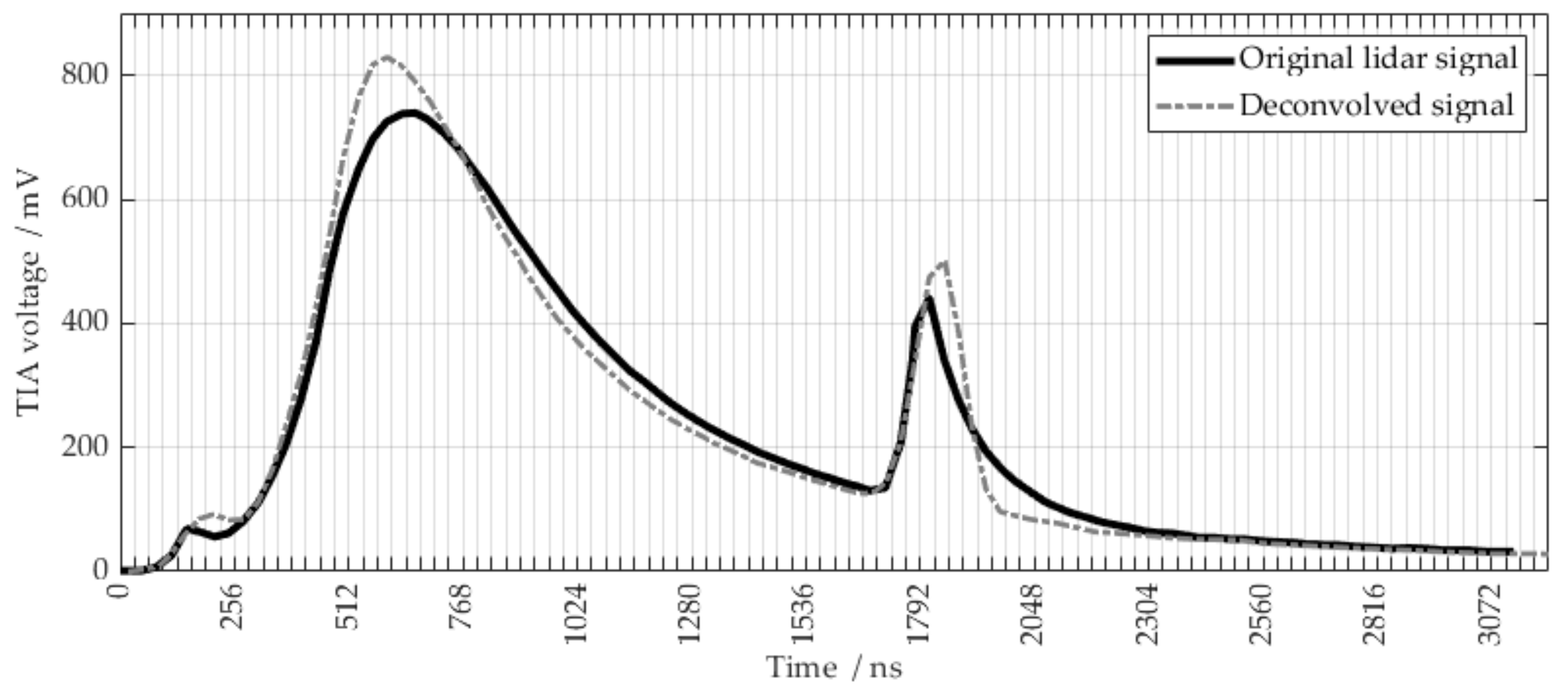
2.3.4. Data Acquisition and Wind Retrieval

As mentioned above, the current signals from the sixteen PMT detector array pixels are converted to voltages by a set of transimpedance amplifier (TIA) circuits. The −3 dB bandwidth of the TIAs is currently implemented with B 3 d B = 1.5 MHz in order to avoid undersampling with the subsequent 31.25 MS/s sampling rate analog-to-digital converter boards. This results in an asymmetric impulse response with a half width of F W H M T I A 110 ns. The digitizer itself features 30 MHz bandwidth and 16-bit resolution.
For our ongoing evaluation purposes, the wind analysis is performed a posteriori, including a series of amplitude (over time) corrections, followed by the spectral evaluation.
The sixteen time-dependent voltages (representing the fringe over range evolvement) are first offset-corrected. The pulse-to-pulse power variation is taken into account by normalization (laser pulse power meter reading) in order not to over-weigh stronger laser pulses in the following. Depending on the required time resolution, several signals (occurring every 10 ms) are summed, as in the following example, 2, 3, 5, 10, 40 or 100 signals, resulting in rates of 50, 33, 20, 10, 2.5 and 1 Hz for our laser with 100 Hz repetition rate. Then, the laser reference and atmospheric signals are separated, depending on how the former is inserted (delayed by the fiber delay line or by a common mirror reflection, when used). Both are then corrected by an individual illumination function that is currently determined for each range interval. The determination of this illumination and detection response function is performed in between wind measurements by sweeping the laser over the whole FSR of the interferometer. This is roughly equivalent to a white light response of the spectral analyzer/receiver back-end. We desist here from a thorough description of this process and its intricacies since exhaustive studies are still ongoing for its optimization.
In order to correct for the required long impulse response of the TIA, a special deconvolution correction (illustrated in Figure 6) is performed at this point. Each of the sixteen time signals is convolved with an optimized kernel (by a method developed for a spaceborne lidar [53]) in order to retrieve the actual range-time resolution; here, a 30 m resolution is implemented. The respective averaging over range time (aggregating samples over range) is performed with an amplitude-dependent weighing in order not to over-weigh close ranges.
Then, the fringe form over the sixteen channels is evaluated for the wind determination. The fringe amplitude (over the channels) has the approximate form of a cosine with skewness and kurtosis, resulting from imperfections of the interferometer and other optical surfaces, the (admittedly quite simplistic) imaging (resulting in aberrations such as a strong pincushion distortion) and, in particular, the above-mentioned illumination function. The Doppler wind information is determined from the phase between reference and atmospheric fringes, for each aggregated time and range lidar averages. These shifts are in the order of 5.6 MHz for a wind speed of 1 m/s according to Δ ν D o p p l e r = 2 v L O S / λ l a s . This resolution corresponds to a fraction of roughly 1/1900 of the free spectral range of the FW-FIMI. This implicates a needed sub-pixel resolution of better than 10 milli-pixels.
Thus, each fringe is approximated by a function of following form:
f ϕ = p A m · 1 + p C o · cos ϕ + sin 1 p K u · sin p S k ϕ p Δ ϕ
where p A , p C o , p K u and p S k are the fit parameters for amplitude, contrast, kurtosis and skewness, respectively. ϕ is the fixed phase of each fringe, while p Δ ϕ is the searched phase deviation due to the Doppler shift with a fixed relationship:
Δ ϕ 2 π = Δ ν D o p p l e r F S R · n p
where n p is the number of the fringe periods imaged onto the illuminated detector pixels.
For approximating the lidar’s fringe data by the above Equation (9), several algorithms have been evaluated. The centroid method [54] and a Gaussian correlation algorithm, i.e., the maximization of the correlation function with a Gaussian [55], both produce large systematic errors, that additionally increase linearly with wind speed (a phenomenon called “slope error”). A thorough analysis based on synthetic data procured by the end-to-end simulator of Section 2.2 is provided in appendix C.8 of [38] for idealized cosine-shaped fringes ( p K u = p S k = 0 in Equation (9)) and skewed and asymmetric fringes.
Therefore, a downhill simplex algorithm fit (DSA, Nelder–Mead method [56]) is applied which showed, so far, the best performance. This scheme does not use derivatives and therefore converges very safely. The results shown below (Section 3) have been derived with the DSA method.

2.3.5. DWL Demonstrator Summary and Note

The above sections describe the Doppler wind lidar demonstrator AEROLI based on the fringe-imaging Michelson interferometer used as spectral analyzer. It must be affirmed that its prime mission is the demonstration of this concept’s functionality in terms of wind measurement. It should be obvious from the given details that a number of concessions had to be made in order to obtain a working system in finite time and budget. In other words, this demonstrator is by no means meant for the direct involvement in the described mission of airborne wind measurement for gust alleviation. Rather, it shall (a) demonstrate the ability of measuring wind with the FW-FIMI concept; (b) validate the simulators (Section 2.1 and Section 2.2) used for the general simulative optimization of the lidar for GLA in terms of specification optimization (see Introduction); and (c) help work out the critical technological elements that must be addressed in more detail to significantly improve the overall performance. The following section will show that this demonstrator very satisfactorily served these three purposes.
Here, we summarize the main shortcomings that distinguish this demonstrator (as of now) from an airborne wind lidar for use in GLA:
  • Use of only one polarization instead of unpolarized (rather arbitrarily polarized) light due to the imperfect beam splitter coating within the FIMI;
  • Implementation of only the transmitted channel of the FIMI;
  • Photon loss and crosstalk on the PMT detector array;
  • Non-optimized overlap integral on very short ranges between transmit beam and telescope receiver field of view due to mono-static co-axial setup, small laser beam divergence and fiber étendue neglection;
  • Simplistic imaging optic setups resulting in image aberrations;
  • Diverse non-optimized optical surfaces (mirrors, fiber facets) resulting in losses;
  • Deficient thermal stabilization, particularly of the FIMI compartment as well as the whole receiver back-end setup;
  • Limited fiber scrambling/inchoate use of the potential of fiber scrambling possibilities; and
  • Unexploited potentials in terms of routines (e.g., illumination function determination procedure) and retrieval methods (fringe function approximation).
This list is not yet exhaustive but highlights the limitations of this demonstrator. Table 2 quantifies the main variables that are used in the simulation (Equation (8)) for the demonstrator in contrast to the ones used for Figure 1, provisionally assessed as feasible for a fully optimized system.
The optical efficiency η o p t of our AEROLI receiver was assessed in a dedicated measurement and by far did not meet the theoretically budgeted 5.8% (slightly corrected value as reported in Chapter 5.3 of [38], there including the detector quantum efficiency). We assume (and could at least partly confirm in later test series) strong misalignments of the front-end telescope-to-fiber coupling as the primary cause. This value has to be considered with care since it yields a large uncertainty, difficult to assess itself. The values for a future achievable implementation (hypothesized) have also been detailed in a lidar feasibility study [18] carried out for RTCA (Radio Technical Commission for Aeronautics).
Comparing these versions, it is obvious that the spectral analyzer coefficients κ i (acting linearly in Equation (8)) alone cause a deterioration (with respect to the projected or “ideal” case) factor of 2.5, whereas the optical efficiency makes for a factor five. This may only be counteracted by our today overdesigned (in terms of P.A.P. and corresponding size, weight and power) laser/receiver system (8 W power and 140 mm telescope, with a 13% obstruction ratio due to the secondary mirror).
The next section highlights the demonstration measurements for the proof of the above points: (a) wind measurement ability and (b) simulator validation.

3. Comparative Analysis of Wind Measurement Performance

In order to assess the actual performance of the Doppler lidar receiver in terms of wind measurement, two ground-based test campaigns were performed in summer 2017 and early winter 2018 at the DLR Oberpfaffenhofen (southern Germany).
Now, as with most remote sensing instruments, the inherent challenge arises as to assess the actual “real” value of the measurand—in our case, the movement of the air (and suspended aerosols) in the direction of our instrument (LOS direction). In the absence of appropriate wind tunnels due to size restrictions (not speaking of astronomical costs) that would deliver calibrated airflow, as all wind lidar developers, we use the naturally occurring wind. This has to be considered somewhat random (which it is not completely), and occurs only in a restricted magnitude range. For instance, such a setup makes it difficult to assess the system’s response to wind values ranging from 0 m/s to 10 m/s, in 1 m/s steps—values typically of high interest. This aspect of the arbitrary measurand, at the mercy of meteorological conditions, is the one challenge. (Please note that there are workarounds for establishing controlled moving scatterers, inter alia, by employing moving hard targets. We ourselves employed such a technique with a linearly moving belt sander [38] that, on the other hand, leads to inevitable other complications, such as increased speckles or point instead of volume measurement, which eventually exacerbate the comparability with atmospheric measurements.)
The other, as a direct consequence of the first, is the question of the reference instrument that quantifies this unsteady wind in a precise and optimally accurate way (for quantifying the uncertainty of both measurements), with the required resolutions (in terms of range, repeat rate) at the required distance (or location). Typical metrology guidelines suggest exploiting a reference instrumentation with a tenfold (if need be threefold) or so better performance (e.g., in terms of precision) than the “device under test” (DUT) in order to be able to neglect its contribution.
In this work, we foremost seek to estimate the possible performance of the DUT (our DWL demonstrator) in terms of standard deviation of the wind measurement in order to compare to Equation (8)-like theoretical estimates. Yet, we are certain to not be able to find such instrumentation regarding these requirements (both settings and uncertainty).
As a baseline, we may utilize a technical state-of-the-art in order to manifest the relation to the “wind-measuring community”. Therefore, we operate a commercial Leosphere/Vaisala Windcube®, coherent DWL, as the reference instrument. Being skeptical scientists, we further use (also commercial) sonic anemometers for backing up these measurements. The limitations of this approach are discussed in the later sections.

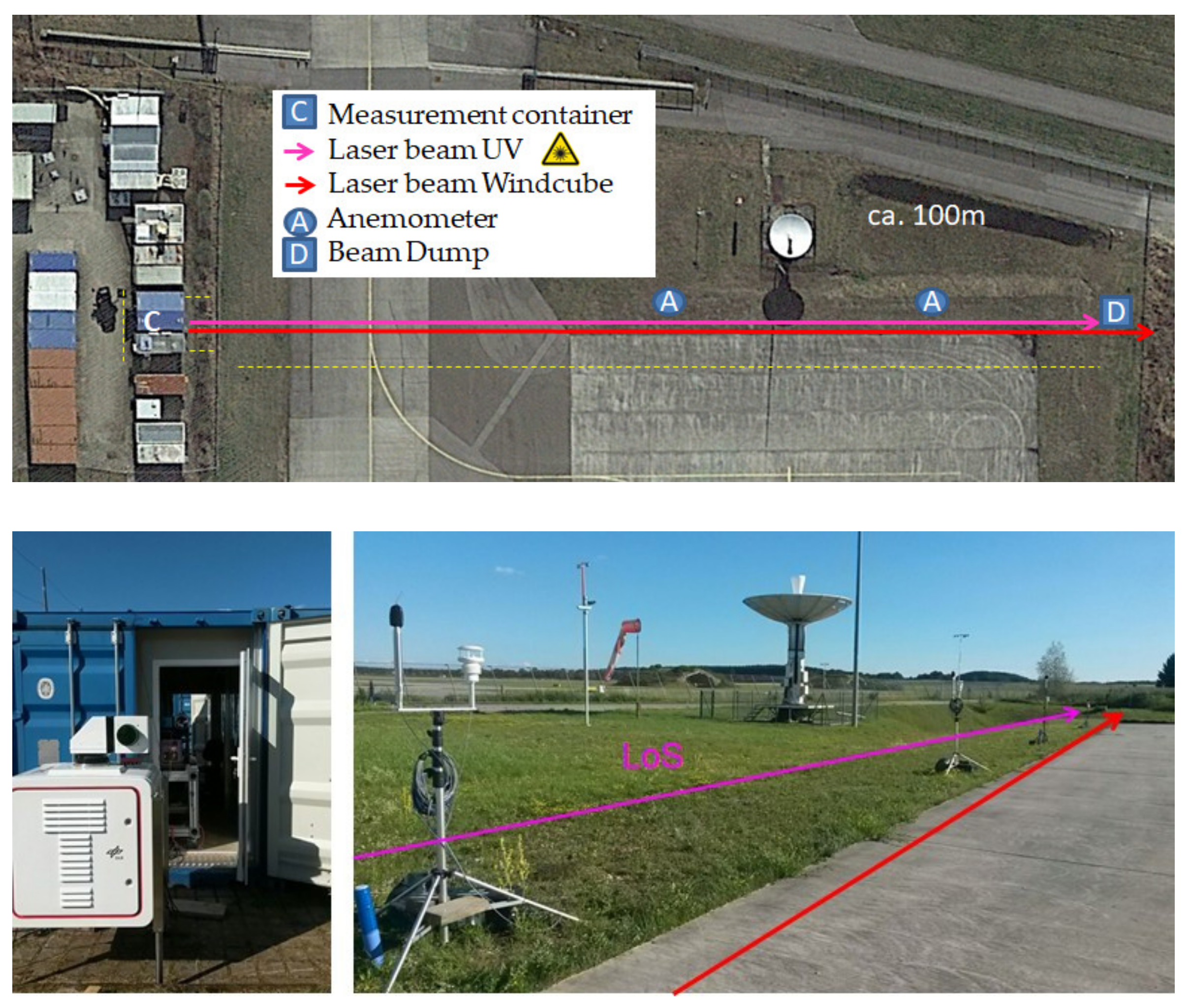
3.1. Measurement Campaign Setup

For this first test campaign, following requirements were formulated:
  • Deployment of demonstrator lidar in a controlled environment (for ease of implementation);
  • Laser beam operation in non-eye-safe conditions;
  • Intervention on laser/lidar beam for hard target measurement and laser beam angular fluctuation analysis (due to inherent instability and local turbulence);
  • Control of Windcube® wind measurements by sonic anemometers; and
  • Possibility of performing also vertical wind measurements.
For meeting these needs, a ground-based campaign was arranged using as a basis a 20-foot shipping container converted to a laboratory (that had been used during various DLR lidar test campaigns), equipped with air conditioning. This lab container is actually “parked” at DLR Oberpfaffenhofen with access to the DLR flight experiments department’s (FX) apron (as visible in the upper panel of Figure 7). The implicit limited access authorization to the air operations area was convenient to operate the high-power laser that features a NOHD (nominal ocular hazard distance) of around 150 m. Both lidars were arranged such that their beams pointed horizontally, close together (<1 m distant), close above the ground (<1 m). The latter was necessary due to the container height, the installation of anemometers, the manual access to the beam and the need to feed the UV beam into a dump after a stretch of ≈100 m. A longer experimental stretch was not available such that actually only two useful range bins (see below) could be evaluated in horizontal mode. For longer range operation, a common transmit/receive 45° mirror was used in front of the AEROLI demonstrator telescope, while the Windcube® may point to any direction.
As mentioned, the Windcube® wind measurements were verified against two sonic anemometers of different models, a Vaisala WXT520 (at 67 m) and a Svantek 181 (at 75 m). The difficulty is the disparity between volume (lidar) and point measurements as well as the partly incompatible time constants of the measurements. However, since a Pearson correlation coefficient of 0.92 and a standard deviation of the difference of 0.5 m/s between the datasets could typically be found, the Windcube® was assessed as reliable as the sole reference for all further analysis (Appendix A of [38]). Table 3 shows the manufacturer’s specifications of the utilized model Windcube® 200S according to the specific user guide [57]. Within scientific literature, somewhat better precisions for the Windcube® series have been reported by the developers, such as a standard deviation of 0.34 m/s as compared to a VHF radar [58] or “accuracy and precision of the radial velocity of 0.1 m/s and 0.2 m/s, respectively” based on calibrated cup anemometers [2]. However, the closeness to the usable bounds of the system (at 50 m distance) with an overlap integral optimized for longer ranges entails rather low values of the system’s CNR (carrier-to-noise ratio), a measure that the Windcube® delivers. We further encountered episodes of apparently low aerosol content (even close to the ground) visible as generally reduced CNR and loss in contrast within the FW-FIMI. Therefore, one should remain cautious about this value.

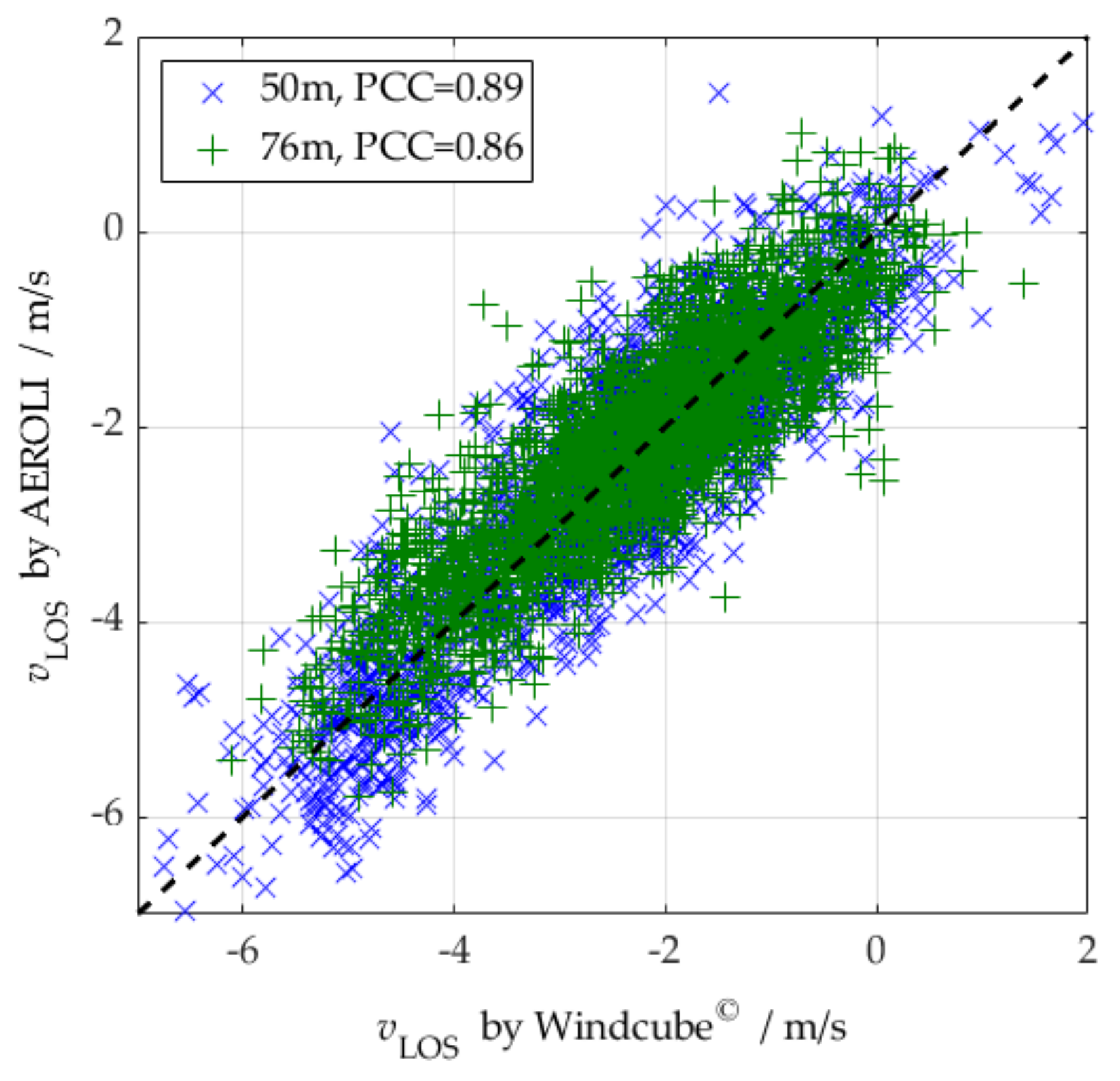
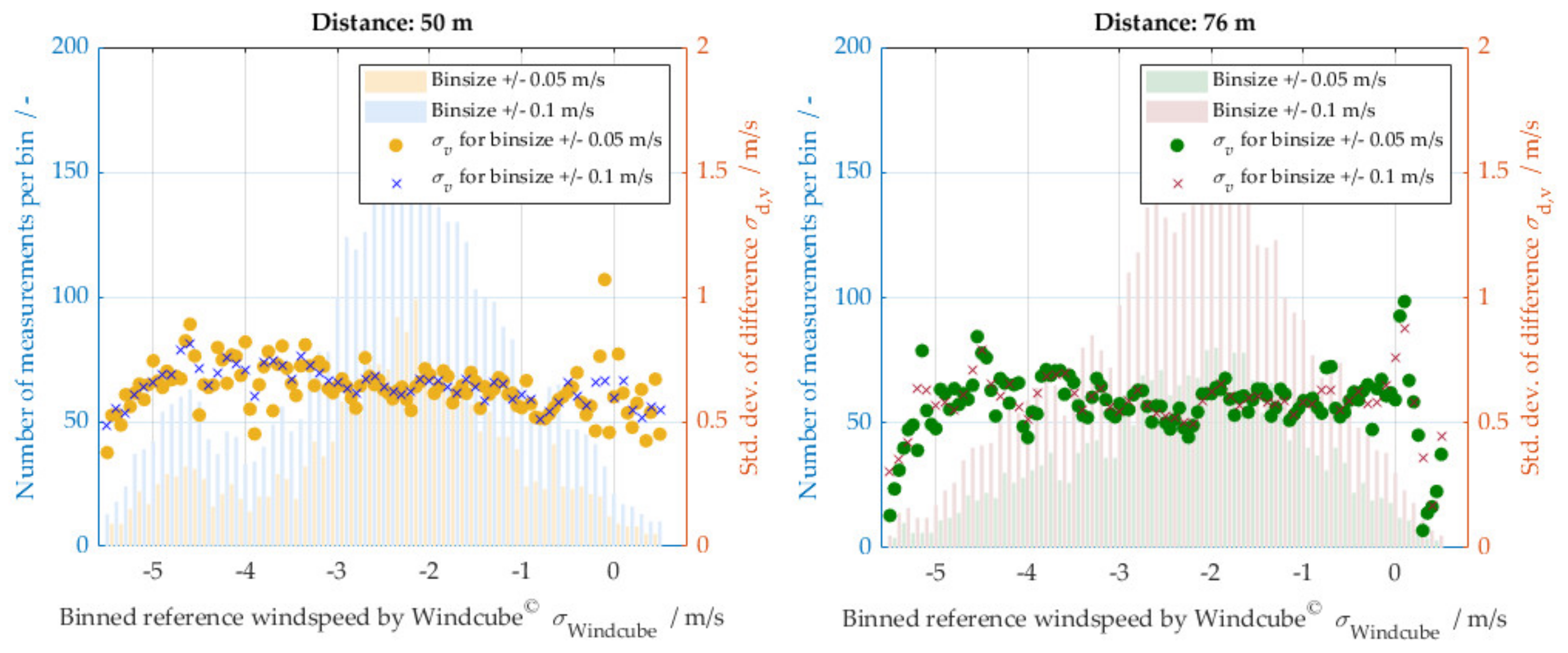
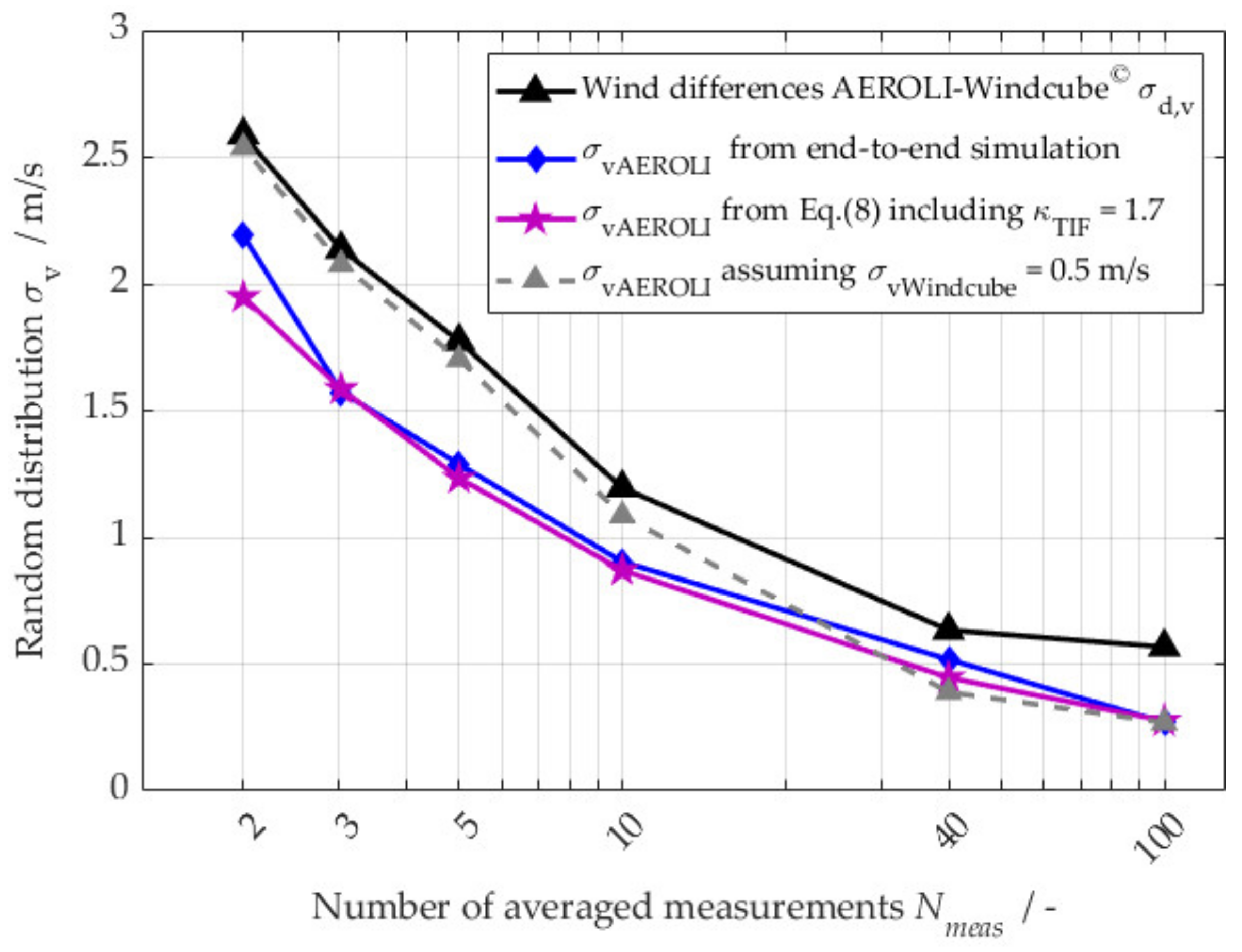
3.2. Wind Measurement Comparisons and Analysis

As mentioned above, two sessions of some weeks of parallel measurements of anemometers, coherent DWL and our FW-FIMI demonstrator were performed between July 2017 and January and March 2018, respectively. Whereas the 2017 series mainly served for trouble-shooting and improvement identification, the 2018 series led to a comprehensive set of wind measurements. Here, all sorts of examinations were performed, including the use of different scrambling fibers and their vibrations, the laser being locked to its iodine reference (high frequency stability) or free-running, overlay of the laser reference pulse by fiber or by hard target (fiber coupler, the beam “dump” at 115 m distance, or the 45° mirror for vertical operation) and of course, meteorological conditions.
In the following, we focus on wind measurement sets obtained on 29 January 2018, throughout the day, since both lidar systems yielded the best common performance (in terms of the difference between their wind measurements, as below).
Regarding our demonstrator system, the laser reference signal was inserted temporally after the close ranges of 50 m and 76 m that are examined here, such that a time signal as depicted in Figure 6 ensued. This certainly leads to some error in the estimation of the actual reference fringe phase due to the superposition of reference and atmosphere return, where the latter still has some non-negligible amplitude. For this series, the laser was both operated locked and free-running, the latter allowing us to conveniently center the fringe on the detector, but coming about with higher frequency drifts.
Concerning the fringe evaluation (cf. Section 2.3.4), forty lidar signals were aggregated as a temporal average (i.e., a refresh rate of 2.5 Hz), and six adjacent range bins were combined to a spatial average of 30 m (numerically actually 28.78 m for the 31.25 Hz sampling rate). What is considered as a “range” here is the geometrical center of this 30 m long volume. As described in Section 2.3.4, the approximation of the fringes’ curve shapes by Equation (9) with the DSA method gives the phase difference between the reference and the atmospheric fringe, leading to the wind speed.
The Windcube® was set to 0.5 s averaging (accumulation) time, 25 m range resolution with 100 ns laser pulse length.
In order to compare AEROLI and Windcube® measurements, both time series had to be re-interpolated onto a common time frame (both are referenced to as UTC time by GPS), which certainly generates an additional error on the difference evaluation. For numerical evaluation, the difference d v between these re-interpolated values is taken and analyzed with standard deviation σ d v :
d v t i n t = v L O S , A E R O L I t i n t v L O S , W i n d c u b e t i n t
σ d v 2 = 1 N i = 1 N d v , i d v 2
where N is the number of the differences and d v is the mean of this difference set.
The series with lowest found standard deviation of the difference σ d v was taken at 19:19 h UTC and is plotted in Figure 8.
A prominent, immediate and somewhat troubling finding is the that all AEROLI measurement sets contain a range-dependent bias (of several m/s), additionally slowly varying over time. This offset bias at least predominantly seems to be a consequence of the limited measurement accuracy of the illumination function determination procedure (Appendix A of [38]). Its distance dependence is assumed to be related to inchoate scrambling of the angular information (as mentioned at the end of Section 2.3.5), whereas its temporal variability to be related to the thermal stability of the FW-FIMI setup. Bias values of −2.7 m/s and −3 m/s for 50 m and 76 m distance, respectively, are already subtracted in Figure 8.
In this context, it must be noted that the projected application within the airborne forward wind sensing does not necessarily require a bias-free wind sensor since such offsets (in absolute value and over range) may readily be handled with online calibration or within the maximum-likelihood estimator of the wind reconstruction algorithm. A time dependence, however, remains critical when the related time constant is short. However, even for our thermally imperfect system, this time constant seems to be in the order of some minutes (>10 min). These advantages of the application will not hinder us to try to ameliorate this aspect as well, though.
Several such comparative series were obtained on that day, with some different AEROLI setups. They are exhaustively reported in [38], and their numerical results are summarized in Table 4.
On that day, the CNR of the Windcube® remained rather low, increasing only towards the later hours (Figure A4 in [38]). Thus, Windcube® measurements below the threshold of CNRmin = −29 dB were excluded, a commonplace method. Since the Windcube®’s wind precision is related to the CNR, it is difficult to say whether one should reckon different values for σ v W i n d c u b e over the day. From this, one might infer a dependency, but this would be nonscientific. Furthermore, there remain many intricacies related to our demonstrator system.
Yet, since the respective wind measurements of AEROLI and Windcube® are statistically independent, we may separate their random errors by the variances, assuming a constant value for σ v W i n d c u b e :
σ d v 2 = σ v A E R O L I 2 + σ v W i n d c u b e 2
Thus, when using the conservative value of Table 2, or of the reference [2] for σ v W i n d c u b e , and the values of σ d v for the distances of 50 m and 76 m, we find:
Conclusion 1.
The random distribution of wind measurements of the FW-FIMI demonstrator achieves values in a range as low as 0.4 to 0.65 m/s, yielding:
σ v A E R O L I 0.5   m / s   for   averages   of   40   pulses   and   30   m   length
The correlation (after Pearson) of the two measurement sets, by AEROLI and the Windcube®, gives coefficient values of 0.89 and 0.86 at the two analyzed distances, respectively (cf. Figure 9).
In order to determine a possible dependency of the derived wind speed on the magnitude of the values itself (i.e., the slope error, referred to in Section 2.3.4 regarding different methods of fringe fitting), the AEROLI wind values v L O S , A E R O L I t i n t are sorted based on their physical value (assuming the Windcube® as the universal unbiased reference, thus after v L O S , W i n d c u b e t i n t ) in bin sizes of ±0.05 m/s and ±0.1 m/s. Then, the respective differences (between AEROLI and the Windcube® “truth”) within each bin are calculated, and then the standard deviation of the set.
This standard deviation should approximately equal the one determined for the whole set of 15 min measurement time. Figure 10 confirms that this is actually the case for both bin lengths (dots and crosses). The histograms (number of occurrence of specific value) in the background highlight the inherent difficulty of the approach using natural occurring wind, as laid out above: for extreme values, there are so few datapoints, that the determined standard deviation value (which should be around 0.6 m/s) becomes very unreliable and should thus not be considered (e.g., occurrence of less than 20 times).
Within these limits, though, we may stipulate:
Conclusion 2.
No significant slope error, i.e., a dependence of the wind speed uncertainty on the observed wind speed, was found in addition to (and the presence of) the random error.
Lastly, we analyze the wind speed determination fluctuation of the FW-FIMI prototype AEROLI depending on the averaging duration. For this purpose, the first step of averaging ( N m e a s ) is executed for only two laser (lidar) pulses (signals), for 3, 5, 10 and 100. All other evaluation steps are carried out as before. Here, the same dataset as above (29 January 2018 19:19 h) is used. In Figure 11, the respective results of the differencing after Equations (11) and (12) in terms of standard deviation σ d v are plotted over this number of measurement averaging N m e a s (triangles, bold black). The gray dashed line (triangles) indicates a possible performance of the AEROLI DWL when assuming σ v W i n d c u b e = 0.5 m/s in applying Equation (13).
Blue diamonds indicate the results of the end-to-end simulations (Section 2.2), based on the demonstrator system parameters given in Table 2, as well as cautious estimations of the backscatter ratio Rb, based on fringe contrast measurements (and underpinned by CNR values) and local air temperature. The same (for Rb) is carried out for the simple determination of σ v A E R O L I after Equation (8), and with κ T I F = 1.7 (Table 1), drawn as purple stars.
It is clear that the purple curve shape simply follows the rule of improvement of a statistically independent set of measurements with the number of averaged measurements by 1 / N m e a s . The end-to-end simulation also follows this form for the most part, since it contains random but independent processes. Noise filtering seems to play a minor role. The deviation from the model after Equation (8) at N m e a s = 2 may also be due to too few realizations (“unluckily pessimistic”). The value κ T I F = 1.7 makes for the best adaptation of Equation (8) to the end-to-end simulation. The actual attribution of the respective error sources to the different technical modules (i.e., κ T I F split in Figure 2) is pending and will be analyzed in the future.
Regarding the measurement performance, it may be deduced from Figure 11 that the σ v W i n d c u b e -corrected curve (gray triangles) coincides well with the modeled performance for higher number of averages ( N m e a s = 40 and 100). Generally, there seems to be a floor for the σ d v values of ≥ 0.5 m/s at high numbers (no more improvement), eventually designating the end of this method.
For lower N m e a s 10 , the curves clearly deviate, but not by more than 0.5 m/s, a fraction only of the respective random distribution. This non-white noise behavior may be attributed to poor averaging, possibly of speckles (affecting the fringe form). It is not surprising that a higher number of N m e a s performs better (apart from the pure number), and it is significant information that this range of some tens to possibly a few hundred pulses is a good value for a future optimized system for the GLA application. It may in general be stated that the concordance between measurement (corrected or not) and model is quite satisfying, thus:
Conclusion 3.
The simulation models, both simple analytic after Equation (8), as well as the end-to-end model, reproduce the measurements for different averaging conditions in a very satisfactory way. Thus, both seem adequate to be used for modeling the performance of such a DWL system.
This last finding is of particular importance for the validated overall simulation of the airborne GLA application including the lidar system, gust reconstruction, aircraft model and controller.

4. Discussion

4.1. Reciprocal Validation and Confirmation of Approach

As pointed out above, the development of the AEROLI demonstrator based on the FW-FIMI has the dual purpose of the validation of the developed simulators (and vice versa) and the technological advancement in itself.
From the highlighted Conclusions 1–3, we may infer that the first objective is thoroughly met. The end-to-end simulator satisfactorily reproduces the performance, as determined with the comparative wind measurements for various averaging settings, as shown in Figure 11, particularly for higher averaging numbers N m e a s of some tens to hundreds. These higher numbers N m e a s are explicitly interesting for higher pulse rate (PRF) laser systems. Both the wind measurement performance and the end-to-end simulation results (in terms of random distribution of retrieved wind value) are “only” a factor of κ T I F = 1.7 away from the theoretical physical limit (the Cramér–Rao lower bound), basically given by Equation (8). The term “only” may be regarded as quite euphemistic as this still corresponds to a factor of three in photon number for compensation. However, since this AEROLI demonstrator of 2018 merely represents a first shot, this may be regarded as quite encouraging.
In the broader context of the application, previous holistic studies of the lidar-based GLA control scheme, such as [20], have recently been confirmed and reforged by employing the lidar model as in Equation (8). Utilizing the hypothetical—yet in the future, attainable—set of parameters as given in Table 2, considerable load reductions for aircraft structures could be shown [59] through the full simulation suite: “the designed lidar-based gust load alleviation system exhibits excellent qualitative behavior and an excellent load alleviation performance. The controller was able to reach and even exceed the target of 10% maximum bending moment reduction on all wing stations but the wing tip, for which the critical gusts are too small to be detected via the lidar sensor”. Furthermore, this control system “improves the loads and margins at almost all stations”. A bending moment reduction, which is the primary wing structure design driver, of more than 10% is of considerable interest since it would allow a significant reduction in this structural mass.
Regarding the technological advancement of a DD-DWL, we are now reassured that this remote sensing technology, the FW-FIMI architecture, is a suitable choice and merits further pursuit.
Admittedly, the illumination and response function of the FIMI, connected to the fringe-imaging approach, remains a challenge at present (we touched on that subject only superficially here). Our present setup requires repeated re-calibration (currently by sweeping the laser through the FSR, what may not be available for other laser developments), which we suspect is a significant cause for the bias in the measurement. However, it cannot be excluded that similar effects are observed also for non-FI approaches.
The next section will summarize the main technological points to be tackled.

4.2. Ongoing and Future Orientations

From Section 2 and Section 3, it is evident in which dimensions this demonstrator must be improved in order to pave the way for future industrial adoption: in terms of measurement precision and in absolute accuracy (regarding bias).
The precision should be improved in a relative and an absolute way. Relative, meaning the augmentation of the SNR by increasing the system’s photon throughput, quantified by the optical efficiency η o p t . Such effort may be regarded as “simple” engineering tasks, as with using advanced coatings, optimizing couplings, alignments and the overlap. Moreover, optimized fiber core materials for UV use should be studied, and the fiber lengths optimized. Additionally, the second, back-reflected channel shall be implemented, followed by a FIMI with optimized beam splitter, i.e., with a splitting ratio invariant to polarization state.
Improving the system’s wind speed determination precision in an absolute manner mainly refers to the decrease in the here-introduced “technology implementation factor” κ T I F . This shall be achieved by the optimization of imaging optics (reducing aberrations), the fringe form, and the retrieval routines. Moreover, the combination of reference and atmospheric return light shall be improved.
Finally, the bias should at least be stabilized to a constant value that may be calibrated. To this end, the illumination and response function shall be stabilized, in terms of simple thermally induced drift, as well as by a rigorous improvement of the scrambling of geometry information (i.e., in terms of lateral field and distance angle). The determination of this function must be optimized in order to not hamper the wind speed measurements, and to provide more precise and accurate information. Last, the fringe approximation methods shall be reviewed and extended, in terms of calculation performance and robustness.
Finally, as we have been addressing some of the shortcomings of the described methods of DWL evaluation and testing, there should be more thorough test concepts. In particular, we have been lacking the information of the backscatter ratio Rb or the backscatter coefficients for accounting of several effects. This may be helped by a set of aerosol (possibly in situ) measurement devices. Then, a wind reference with higher data repeat cycles than provided by the Windcube® would be advantageous when analyzing high-rate AEROLI wind data.
In an abstract way, the error (propagation) on all the presented quantities should be addressed in detail—a “detail” that could not be analyzed here due to lacking information in that matter.

5. Conclusions

Recapitulating the explained aspects, we conclude that this present technology of a Direct-Detection Field-Widened Fringe-Imaging Michelson DWL performs very close to theoretical expectations that are materialized by end-to-end simulations and the Cramér–Rao lower bound.
The embedment of these simulations in overarching full lidar-based GLA control simulations fundamentally validates the concept of DD-DWL for this purpose.
This DD-FW-FIMI demonstrator is systematically worked on to evolve its precision, accuracy and efficiency, with the body of knowledge growing.

Author Contributions

Conceptualization, P.V.; methodology, P.V. and J.H.; software, J.H. and P.V.; validation, J.H.; formal analysis, J.H.; investigation, J.H. and P.V.; resources, P.V.; data curation, J.H.; writing—original draft preparation, P.V. and J.H.; writing—review and editing, P.V.; visualization, P.V.; supervision, P.V.; project administration, P.V.; funding acquisition, P.V. All authors have read and agreed to the published version of the manuscript.

Funding

Part of the work has been funded within the framework of the European CleanSky2 Joint Technology Initiative–Airframe (grant agreement number CS2JU-AIR-GAM-2014-2015-01 Annex 1, Issue B04, 2 October 2015) being part of the Horizon 2020 research and innovation framework programme of the European Commission.

Data Availability Statement

Data may be obtained from the author(s) on request.

Conflicts of Interest

The authors declare no conflict of interest.

References

  1. Willis, D.J.; Niezrecki, C.; Kuchma, D.; Hines, E.; Arwade, S.R.; Barthelmie, R.J.; DiPaola, M.; Drane, P.J.; Hansen, C.J.; Inalpolat, M.; et al. Wind Energy Research: State-of-the-Art and Future Research Directions. Renew. Energy 2018, 125, 133–154. [Google Scholar] [CrossRef]
  2. Thobois, L.; Cariou, J.P.; Gultepe, I. Review of Lidar-Based Applications for Aviation Weather. Pure Appl. Geophys. 2018, 176, 1959–1976. [Google Scholar] [CrossRef]
  3. Zheng, J.; Sun, D.; Chen, T.; Dou, X.F.; Zhao, R.; Li, Z.; Zhou, A.; Zhang, N.; Gao, J.; Wang, G. Wind Profiling from High Troposphere to Low Stratosphere Using a Scanning Rayleigh Doppler Lidar. Opt. Rev. 2018, 25, 720–728. [Google Scholar] [CrossRef]
  4. Marksteiner, U.; Lemmerz, C.; Lux, O.; Rahm, S.; Schäfler, A.; Witschas, B.; Reitebuch, O. Calibrations and Wind Observations of an Airborne Direct-Detection Wind LiDAR Supporting ESA’s Aeolus Mission. Remote Sens. 2018, 10, 2056. [Google Scholar] [CrossRef] [Green Version]
  5. Franken, P.; Jenney, J.; Rank, D. Airborne Investigations of Clear-Air Turbulence with Laser Radars. IEEE J. Quantum Electron. 1966, 2, 147. [Google Scholar] [CrossRef]
  6. Vrancken, P. Airborne Remote Detection of Turbulence with Forward-Pointing LIDAR. In Aviation Turbulence; Sharman, R., Lane, T., Eds.; Springer International Publishing: Cham, Switzerland, 2016; ISBN 978-3-319-23629-2. [Google Scholar]
  7. European Aviation Safety Agency (EASA). Annual Safety Review 2013; EASA: Cologne, Germany, 2013; ISBN 978-92-9230-187-9. [Google Scholar]
  8. Federal Aviation Administratuion (FAA). Advisory Circular 120-88A—Preventing Injuries Caused by Turbulence; FAA: Washington, DC, USA, 2006. [Google Scholar]
  9. Flightpath 2050: Europe’s Vision for Aviation; European Commission (Ed.) Policy/European Commission; Publications Office of the European Union: Luxembourg, 2011; ISBN 978-92-79-19724-6. [Google Scholar]
  10. Advisory Council for Aviation Research and Innovation in Europe (ACARE). Strategic Research & Innovation Agenda—Update 2017; ACARE: Brussels, Belgium, 2017. [Google Scholar]
  11. European Commission EGP—European Green Deal—Transport. Available online: https://ec.europa.eu/info/strategy/priorities-2019-2024/european-green-deal/transport-and-green-deal_en (accessed on 28 September 2021).
  12. European Aviation Safety Agency (EASA). Certification Specification for Large Aeroplanes (CS-25); Amendment 3; EASA: Cologne, Germany, 2007. [Google Scholar]
  13. International Air Transport Association (IATA). 20 Year Passenger Forecast. Available online: https://www.iata.org/en/publications/store/20-year-passenger-forecast/ (accessed on 28 September 2021).
  14. Williams, P.D. Increased Light, Moderate, and Severe Clear-Air Turbulence in Response to Climate Change. Adv. Atmos. Sci. 2017, 34, 576–586. [Google Scholar] [CrossRef] [Green Version]
  15. Grewe, V.; Matthes, S.; Frömming, C.; Brinkop, S.; Jöckel, P.; Gierens, K.; Champougny, T.; Fuglestvedt, J.; Haslerud, A.; Irvine, E.; et al. Feasibility of Climate-Optimized Air Traffic Routing for Trans-Atlantic Flights. Environ. Res. Lett. 2017, 12, 034003. [Google Scholar] [CrossRef]
  16. Vrancken, P.; Wirth, M.; Ehret, G.; Barny, H.; Rondeau, P.; Veerman, H. Airborne Forward-Pointing UV Rayleigh Lidar for Remote Clear Air Turbulence Detection: System Design and Performance. Appl. Opt. 2016, 55, 9314–9328. [Google Scholar] [CrossRef] [Green Version]
  17. Bellamy, W. Boeing to Use LIDAR for Industry First on EcoDemonstrator. Aviation Today 2018. [Google Scholar]
  18. Sishtla, V.; Kameyama, S.; Finley, J.; Gidner, D.; Nguyen, L.; Hofmann, K.; Berthier, J.B.; Lefez, T.; Xiao, Z.F.; Koch, G.; et al. Feasibility Study: Airborne LIDAR for Clear Air Turbulence Detection; RTCA Inc.: Washington, DC, USA, 2020; p. 108. [Google Scholar]
  19. Fezans, N.; Schwithal, J.; Fischenberg, D. In-Flight Remote Sensing and Identification of Gusts, Turbulence, and Wake Vortices Using a Doppler LIDAR. CEAS Aeronaut J. 2017, 8, 313–333. [Google Scholar] [CrossRef] [Green Version]
  20. Fezans, N.; Joos, H.-D.; Deiler, C. Gust Load Alleviation for a Long-Range Aircraft with and without Anticipation. CEAS Aeronaut J. 2019, 10, 1033–1057. [Google Scholar] [CrossRef] [Green Version]
  21. Fezans, N.; Joos, H.-D. Combined Feedback and LIDAR-Based Feedforward Active Load Alleviation. In Proceedings of the AIAA Atmospheric Flight Mechanics Conference, Denver, CO, USA, 5–9 June 2017; American Institute of Aeronautics and Astronautics: Denver, CO, USA, 2017. [Google Scholar]
  22. Ehlers, J.; Fischenberg, D.; Niedermeier, D. Wake Identification Based Wake Impact Alleviation Control. In Proceedings of the 14th AIAA Aviation Technology, Integration, and Operations Conference, Atlanta, GA, USA, 16–20 June 2014; American Institute of Aeronautics and Astronautics: Atlanta, GA, USA, 2014. [Google Scholar]
  23. Kauffmann, P.-P. Market Assessment of Forward-Looking Turbulence Sensing Systems; DIANE Publishing: Collingdale, PA, USA, 2001. [Google Scholar]
  24. Vrancken, P.; Fezans, N.; Kiehn, D.; Kliebisch, O.; Linsmayer, P.; Thurn, J. Aeronautics Application of Direct-Detection Doppler Wind Lidar: Alleviation of Airframe Structural Loads Caused by Turbulence and Gusts. In Proceedings of the 3rd European Lidar Conference, Granada, Spain, 18 November 2021. [Google Scholar]
  25. Cavaliere, D.; Fezans, N.; Kiehn, D.; Quero, D.; Vrancken, P. Gust Load Control Design Challenge Including Lidar Wind Measurements and Based on the Common Research Model. In Proceedings of the 2022 AIAA Scitech Forum, San Diego, CA, USA, 3 January 2022. [Google Scholar]
  26. Kiehn, D.; Fezans, N.; Vrancken, P. Frequency-domain performance characterization of lidar-based gust detection systems for load alleviation. In Proceedings of the DLRK 2021, Online, 1 September 2021. [Google Scholar]
  27. Kiehn, D.; Fezans, N.; Vrancken, P.; Deiler, C. Parameter Analysis of a Doppler Lidar Sensor for Gust detection and Load Alleviation. In Proceedings of the IFASD 2022, Madrid, Spain, 17 June 2022. [Google Scholar]
  28. Khalil, A.; Fezans, N. A Multi-Channel H∞ Preview Control Approach to Load Alleviation Design for Flexible Aircraft. CEAS Aeronaut J. 2021, 12, 401–412. [Google Scholar] [CrossRef]
  29. Fezans, N.; Vrancken, P.; Linsmayer, P.; Wallace, C.; Deiler, C. Designing and Maturating Doppler Lidar Sensors for Gust Load Alleviation: Progress Made Since AWIATOR. In Proceedings of the AEC 2020, Bordeaux, France, 25 February 2020. [Google Scholar]
  30. Witschas, B.; Rahm, S.; Wagner, J.; Dörnbrack, A. Airborne Coherent Doppler Wind Lidar Measurements of Vertical and Horizontal Wind Speeds for the Investigation of Gravity Waves. In Proceedings of the 18th Coherent Laser Radar Conference, Boulder, CO, USA, 27 June–1 July 2016. [Google Scholar]
  31. Inokuchi, H.; Akiyama, T. Performance Evaluation of an Airborne Coherent Doppler Lidar and Investigation of Its Practical Application. Trans. Jpn. Soc. Aeronaut. Space Sci. 2022, 65, 47–55. [Google Scholar] [CrossRef]
  32. Schmitt, N.P.; Rehm, W.; Pistner, T.; Zeller, P.; Diehl, H.; Navé, P. The AWIATOR Airborne LIDAR Turbulence Sensor. Aerosp. Sci. Technol. 2007, 11, 546–552. [Google Scholar] [CrossRef]
  33. Rabadan, G.J.; Schmitt, N.P.; Pistner, T.; Rehm, W. Airborne Lidar for Automatic Feedforward Control of Turbulent In-Flight Phenomena. J. Aircr. 2010, 47, 392–403. [Google Scholar] [CrossRef]
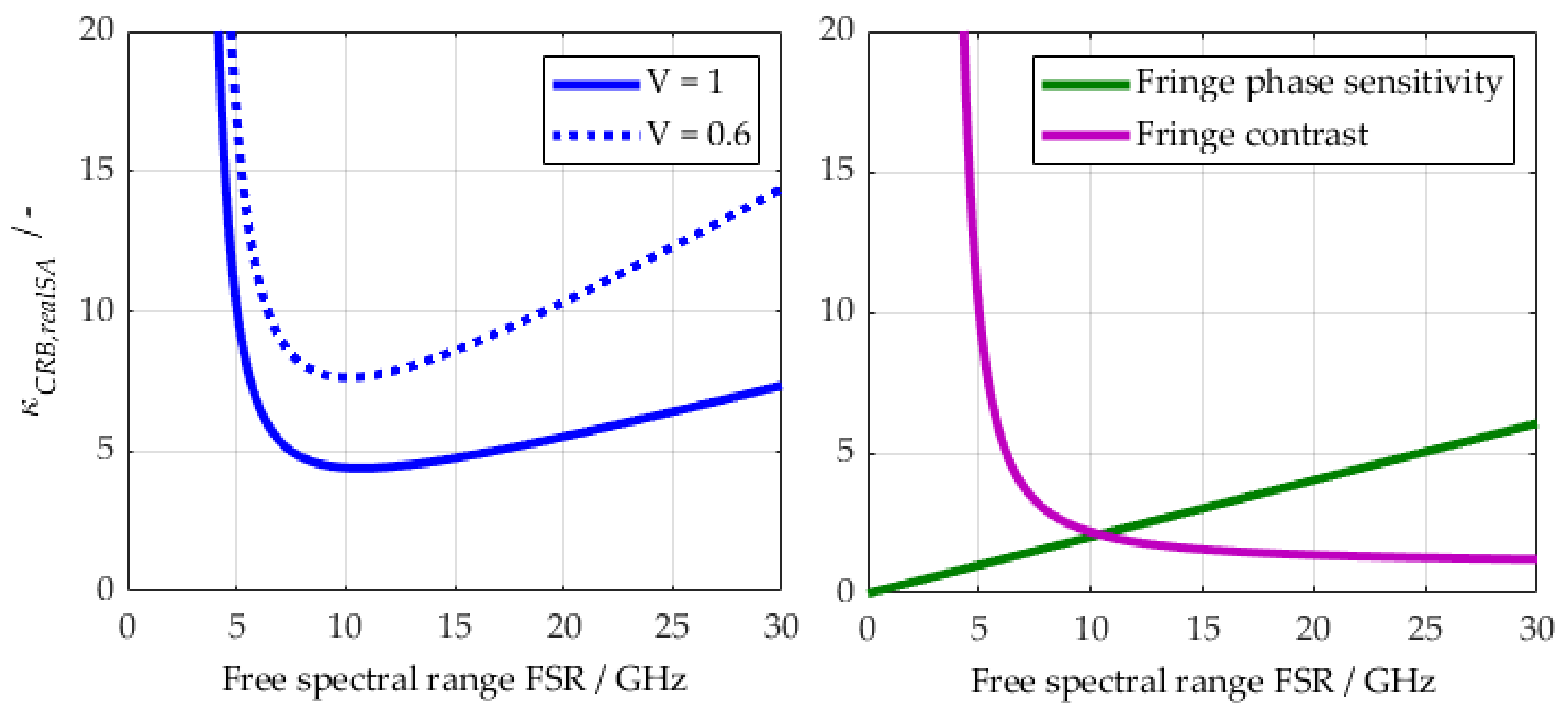
  34. Rye, B.J.; Hardesty, R.M. Discrete Spectral Peak Estimation in Incoherent Backscatter Heterodyne Lidar. I. Spectral Accumulation and the Cramer-Rao Lower Bound. IEEE Trans. Geosci. Remote Sens. 1993, 31, 16–27. [Google Scholar] [CrossRef]
  35. Bruneau, D. Mach–Zehnder Interferometer as a Spectral Analyzer for Molecular Doppler Wind Lidar. Appl. Opt. 2001, 40, 391–399. [Google Scholar] [CrossRef]
  36. McKay, J.A. Modeling of Direct Detection Doppler Wind Lidar I The Edge Technique. Appl. Opt. 1998, 37, 6480–6486. [Google Scholar] [CrossRef]
  37. Cezard, N.; Dolfi-Bouteyre, A.; Huignard, J.-P.; Flamant, P. Development of a Short-Range 355-Nm Rayleigh-Mie Lidar Using a Michelson Interferometer for Wind Speed Measurements. In Proceedings of the Lidar Technologies, Techniques, and Measurements for Atmospheric Remote Sensing III, Florence, Italy, 17–20 September 2007; International Society for Optics and Photonics: Bellingham, WA, USA, 2007; Volume 6750, p. 675008. [Google Scholar]
  38. Herbst, J. Development and Test of a UV Lidar Receiver for the Measurement of Wind Velocities Aiming at the Near-Range Characterization of Wake Vortices and Gusts in Clear Air. Ph.D. Thesis, Ludwig-Maximilians-Universität, Munich, Germany, 2019. [Google Scholar]
  39. McGill, M.J.; Spinhirne, J.D. Comparison of Two Direct-Detection Doppler Lidar Techniques. Opt. Eng. 1998, 37, 2675–2687. [Google Scholar] [CrossRef]
  40. McKay, J.A. Assessment of a Multibeam Fizeau Wedge Interferometer for Doppler Wind Lidar. Appl. Opt. 2002, 41, 1760–1767. [Google Scholar] [CrossRef]
  41. Bruneau, D. Fringe-Imaging Mach-Zehnder Interferometer as a Spectral Analyzer for Molecular Doppler Wind Lidar. Appl. Opt. 2002, 41, 503–510. [Google Scholar] [CrossRef]
  42. Cezard, N. Etude de Faisabilité d’un Lidar Rayleigh-Mie Pour Des Mesures à Courte Portée de La Vitesse de l’air, de Sa Température et de Sa Densité. Ph.D. Thesis, Ecole Polytechnique, Palaiseau, France, 2008. [Google Scholar]
  43. Herbst, J.; Vrancken, P. Design of a Monolithic Michelson Interferometer for Fringe Imaging in a Near-Field, UV, Direct-Detection Doppler Wind Lidar. Appl. Opt. 2016, 55, 6910–6929. [Google Scholar] [CrossRef]
  44. Lidar: Range-Resolved Optical Remote Sensing of the Atmosphere; Weitkamp, C. (Ed.) Springer Series in Optical Sciences; Springer: New York, NY, USA, 2005; ISBN 978-0-387-40075-4. [Google Scholar]
  45. Endemann, M. ADM-Aeolus: The First Spaceborne Wind Lidar; Singh, U.N., Itabe, T., Rao, D.N., Eds.; SPIE Asia-Pacific Remote Sensing Symposium: Goa, India, 2006; p. 64090G. [Google Scholar]
  46. Vrancken, P.; Herbst, J. Development and Test of a Fringe-Imaging Direct-Detection Doppler Wind Lidar for Aeronautics. In Proceedings of the EPJ Web of Conferences, Hefei, China, 24–28 June 2019. [Google Scholar]
  47. Bruneau, D.; Pelon, J.; Blouzon, F.; Spatazza, J.; Genau, P.; Buchholtz, G.; Amarouche, N.; Abchiche, A.; Aouji, O. 355-Nm High Spectral Resolution Airborne Lidar LNG: System Description and First Results. Appl. Opt. 2015, 54, 8776–8785. [Google Scholar] [CrossRef]
  48. Tucker, S.C.; Weimer, C.; Adkins, M.; Delker, T.; Gleeson, D.; Kaptchen, P.; Good, B.; Kaplan, M.; Applegate, J.; Taudien, G. Optical Autocovariance Wind Lidar (OAWL): Aircraft Test-Flight History and Current Plans. In Lidar Remote Sensing for Environmental Monitoring XV; International Society for Optics and Photonics: Bellingham, WA, USA, 2015; Volume 9612, p. 96120E. [Google Scholar]
  49. Tucker, S.C.; Weimer, C. Benefits of a Quadrature Mach Zehnder Interferometer as Demonstrated in the Optical Autocovariance Wind and Lidar (OAWL) Wind and Aerosol Measurements. In Proceedings of the Remote Sensing of the Atmosphere, Clouds, and Precipitation VII, Honolulu, HI, USA, 24–26 September 2018; Im, E., Yang, S., Eds.; SPIE: Honolulu, HI, USA, 2018; p. 13. [Google Scholar]
  50. Grund, C.J.; Eloranta, E.W. Fiber-Optic Scrambler Reduces the Bandpass Range Dependence of Fabry–Perot Étalons Used for Spectral Analysis of Lidar Backscatter. Appl. Opt. 1991, 30, 2668–2670. [Google Scholar] [CrossRef]
  51. Avila, G.; Singh, P.; Chazelas, B. Results on Fibre Scrambling for High Accuracy Radial Velocity Measurements; SPIE: San Diego, CA, USA, 2010; p. 773588. [Google Scholar]
  52. Wirth, M.; Fix, A.; Mahnke, P.; Schwarzer, H.; Schrandt, F.; Ehret, G. The Airborne Multi-Wavelength Water Vapor Differential Absorption Lidar WALES: System Design and Performance. Appl. Phys. B 2009, 96, 201–213. [Google Scholar] [CrossRef] [Green Version]
  53. Wirth, M. MERLIN Algorithm Theoretical Basis Document: Top Level Algorithms for Primary L1/2 Products; DLR/CNES Methane Remote Sensing Lidar Mission (MERLIN) Documentation Base: Cologne, Germany, 2017. [Google Scholar]
  54. Gagné, J.-M.; Saint-Dizier, J.-P.; Picard, M. Méthode d’echantillonnage Des Fonctions Déterministes En Spectroscopie: Application à Un Spectromètre Multicanal Par Comptage Photonique. Appl. Opt. 1974, 13, 581–588. [Google Scholar] [CrossRef]
  55. Paffrath, U. Performance Assessment of the Aeolus Doppler Wind Lidar Prototype. Ph.D. Thesis, Technische Universität München, Munich, Germany, 2006. [Google Scholar]
  56. Nelder, J.A.; Mead, R. A Simplex Method for Function Minimization. Comput. J. 1965, 7, 308–313. [Google Scholar] [CrossRef]
  57. Leosphere WINDCUBE© 100S, 200S, 400S Hardware System v1.3.5 User Guide—Version 6; Vaisala/Leosphere: Paris, France, 2016.
  58. Cariou, J.P.; Thobois, L.; Parmentier, R.; Boquet, M.; Loaec, S. Assessing the Metrological Capabilities of Wind Doppler Lidars. In Proceedings of the CLRC, Barcelona, Spain, 17–20 June 2013. [Google Scholar]
  59. Fezans, N.; Wallace, C.; Kiehn, D.; Cavaliere, D.; Vrancken, P. Lidar-Based Gust Load Alleviation—Results Obtained on the Clean Sky 2 Load Alleviation Benchmark. In Proceedings of the IFASD 2022, Madrid, Spain, 17 June 2022. [Google Scholar]
Figure 1. (Left) panels show the dependencies of Equation (8) on variables for altitude h, range of measurement R, range resolution (or bin length, or range gate length) Δ R and (averaging) refresh rate r refresh . (Right) panels show the same dependencies when (analytically) incorporating electronics noise terms into Equation (8), which is not further addressed here.
Remotesensing 14 03356 g001
Figure 2. Synopsis of the physics-based end-to-end simulation. Black boxes indicate modules of physical or technical processes, blue rounded boxes relate to adjustable inputs. Green rounded boxes refer to the basic variables (variable arrays) handed over between modules. Dot patterns indicate implemented random processes or inputs. More details in the text.
Remotesensing 14 03356 g002
Figure 3. (Left): Artist’s impression of the interferometer imaging scheme. Collimated illumination (from left) by a square beam (fiber tip near field), imaging of resulting linear fringe (intensity distribution in red) by cylindrical and conventional lens on one-dimensional detector array. (Right): AEROLI demonstrator’s monolithic field-widened Michelson interferometer in its Invar caging, left glass arm, right air arm with spacers.
Remotesensing 14 03356 g003
Figure 4. (Left): The Cramér-Rao lower-bound of our implementation of the FW-FIMI for single-channel use as a function of the free spectral range (simplified Figure 1 from [43]). (Right): Competing components of the left figure, the fringe phase sensitivity and the global fringe contrast.
Remotesensing 14 03356 g004
Figure 5. Synopsis of the two subsystems of the DWL receiver. (Left): Telescope with fiber insertion and combination (front-end). (Right): Spectral analyzer receiver back-end with collimation (out of square-core fiber), polarization selection, interferometer illumination (within thermalized housing) and imaging onto detector PMTA. Acronyms in the text.
Remotesensing 14 03356 g005
Figure 6. Sample of one of the 16 electronic outputs of the TIA (black bold). The abscissa shows the 32 ns sample rate. This signal is deconvolved with a Gaussian deconvolution routine for an effective range resolution of 30 m. The first pulse shows the onset due to the overlap function, then the 1/R²-decline. The second pulse is the laser reference inserted with the fiber delay line (Figure 5.7a of [38]).
Remotesensing 14 03356 g006
Figure 7. Setup of the ground test campaigns in 2017 and 2018.
Remotesensing 14 03356 g007
Figure 8. Wind measurement set taken on 29 January 2018, 19:19 h UTC. The upper two panels show the wind measurement by the Windcube® and AEROLI, respectively. The offset bias of the latter has already been subtracted. The lower panel shows the difference in the above measurements, after re-interpolation on a common time frame. The standard deviations of the difference between the two wind lidars are 0.68 m/s at 50 m and 0.64 m/s at 76 distance, respectively.
Remotesensing 14 03356 g008
Figure 9. Correlation of the lidar measurement sets. The regression line is symmetric due to the prior subtraction of the offset-bias.
Remotesensing 14 03356 g009
Figure 10. Analysis of the slope error of wind measurement by evaluating wind bins.
Remotesensing 14 03356 g010
Figure 11. Analysis of the AEROLI demonstrator performance for different averaging times, along with theoretical (simulative) results (modified excerpt from Figure 5.16 in [38]). Details in the text.
Remotesensing 14 03356 g011
Table 1. Penalty factors of wind speed measurements for various direct-detection Doppler wind lidar receiver concepts with respect to an ideal spectral analyzer (ISA). Table C.1 in [38].
Technique (Interferometer)Abbreviation κ C R B realSA Literature
Dual-channel Fabry–PérotDFP2.4[36]
Fringe-imaging Fabry–PérotFIFPI3.1[39]
Fringe-imaging FizeauFIFI2–4[40]
Dual-channel Mach–ZehnderDMZ1.65[35]
Four-channel Mach–ZehnderQMZ2.3[35]
Fringe-imaging Mach–ZehnderFIMZ2.3[41]
Dual fringe-imaging MichelsonFIMI4.4[42]
Oblique-incidence (dual-channel)
Fringe-imaging Michelson
FW-FIMI2.3[43]
Perpendicular-incidence (single-channel)
Fringe-imaging Michelson
4.4
Table 2. Main variables for the performance estimation after Equation (8).
VariableAEROLI DemonstratorOptimized Hypothesis
κ realSA 4.42.3
κ T I F 1.71.3
η o p t 0.9%22%
P . A . P . 100 mWm250 mWm2
Table 3. Relevant performance characteristics of the used coherent DWL Vaisala/Leosphere Windcube® 200S (according to [57]).
ParameterVariable
Accumulation   time   of   measurements   1 / r r e f r e s h 0.5 s to 10 s
Range   resolution   Δ R , physical and processed25 m, 50 m, 75 m, 100 m
Precision / accuracy   of   radial   windspeed   σ v , L O S <0.5 m/s
Minimum   range   of   measurements   R m i n ≥50 m   = 2 · Δ R
Laser   power   P l a s , W C ≤5 mW
Laser   wavelength   λ l a s , W C 1543 nm
Laser   pulse   length   τ l a s , W C 400 ns, 200 ns or 100 ns
Laser   repetition   rate   P R F , depending   on   τ l a s , W C 10 kHz, 20 kHz, 40 kHz *
*: not in [57].
Table 4. Synopsis of the main wind comparison series on 29 January 2018.
Series
(Start Time UTC)
σ d v at 50 m σ d v at 76 mLaser SettingWindcube® CNR
Observation
13:160.83 m/s0.93 m/slockedmedium
16:291.14 m/s1.13 m/slockedlow
16:481.29 m/s1.35 m/slockedlow (>−34 dB)
18:250.77 m/s0.73 m/sfree runninggood (>−28 dB)
19:190.68 m/s0.64 m/slockedgood
Publisher’s Note: MDPI stays neutral with regard to jurisdictional claims in published maps and institutional affiliations.

