Ship Detection in Visible Remote Sensing Image Based on Saliency Extraction and Modified Channel Features

Abstract

Ship detection in visible remote sensing (VRS) images has been widely used in the military and civil fields. However, the various backgrounds and the variable scale and orientation bring great difficulties to effective detection. In this paper, we propose a novel ship target detection scheme based on small training samples. The scheme contains two main stages: candidate region extraction and ship identification. In the first stage, we propose a visual saliency detection model based on the difference in covariance statistical characteristics to quickly locate potential ships. Moreover, the multi-scale fusion for the saliency model is designed to overcome the problem of scale variation. In the second stage, we propose a three-channel aggregate feature, which combines a rotation-invariant histogram of oriented gradient and the circular frequency feature. The feature can identify the ship target well by avoiding the impact of its rotation and shift. Finally, we propose the VRS ship dataset that contains more realistic scenes. The results on the VRS ship dataset demonstrate that the saliency model achieves the best AUC value with 0.9476, and the overall detection achieves a better performance of 65.37% in terms of [email protected]:0.95, which basically meets the need of the detection tasks.

1. Introduction

In recent years, with the rapid development of remote sensing information science, ship detection, as an important part of ocean remote sensing, has been widely used in the military and civil fields. As far as military reconnaissance is concerned, ship targets are important targets for modern naval warfare detection. Accurate detection of ship targets is beneficial for commanders and fighters to obtain military intelligence, adjust firepower deployment, and contribute to the maintenance of maritime rights and the realization of naval strategies. As for the civil field, ship detection and sea area surveillance in specific sea areas and bays can improve coastal defense early warning capabilities, manage water transportation, illegal fishing, illegal smuggling, and illegal oil dumping. A wide variety of sensors are commonly used for these tasks, including the Automated Identification System (AIS), the Vessel Traffic System (VTS), and the Synthetic Aperture Radar (SAR), as well as images within a visible spectrum. AIS and VTS are used to determine the current location of a ship with Very High Frequency (VHF), Global Positioning System (GPS), and Electronic Chart Display and Information System (ECDIS). However, not all the ships are obliged to carry transponders, such as the ships of less than standard tonnage established by the International Maritime Organization (IMO). In addition to tonnage restrictions, some other ships with special purposes often shut down the transceiver deliberately to avoid radar detection. Therefore, remote sensing detection techniques can provide effective means in these situations.

Benefiting from the increasing ability of remote sensing data acquisition of aerospace platforms and the rapid development of high-resolution satellites, more and more remote sensing datasets can be used for research [1]. From the perspective of data acquisition, studies about ship target detection are mainly based on Synthetic Aperture Radar (SAR) images, infrared remote sensing images (IR), hyperspectral images (HSI), and visible remote sensing images (VRSI). Because of the strong transmittance and all-weather imaging, SAR is hardly affected by climate and illumination. However, the unavoidable speckle noise in SAR images also brings trouble to the detection [2]. IR is used to enhance visual effects under weak light conditions, few studies use infrared images to detect ships due to the low signal-to-noise ratio, insufficient structural information, and fewer features [3]. The HSI dataset has rich spectral dimension information, but data collection is difficult and costly. VRSI is easy to observe and understand, and it is more accessible to people. According to the imaging principle and sensor, the resolution of VRSI is generally higher than that of SAR and IR, which means more details can be captured. Combined with AIS, ship detection in the VRSI aims to efficiently complete the task of positioning and identification. Based on the ship target detection task in VRSIs, the following five challenges are proposed in this paper:

• Since the type of ships and sensor parameters are different, the scales of the ship targets are also inconsistent.
• Color, texture, and other factors of the ship cause a low correlation of target grayscale.
• Sea clutter, ship wakes, islands, clouds, and low light intensity may bring some interference to the detection.
• Target rotation causes poor robustness of the relevant feature.
• Huge computation burden for the large-scale remote sensing data leads to the reduction of detection speed.

In order to meet the above challenges, related research has been improving. However, the existing traditional ship detection algorithms are not robust, and most of them can only be implemented under some certain conditions. As deep learning becomes more and more powerful, the algorithms for ship detection using deep learning are gradually emerging. Up to now, the existing ship detection methods can be divided into three categories: attribute-based methods, traditional supervised learning-based methods, and deep learning-based methods. As for the attribute-based methods, the detection is based on the templates and the contour of the targets [4]. For instance, Harvey [5] proposed an improved ship-template matching method, which used the Hit-or-Miss transform to design a template for matching. However, when the type or direction of the ship is different, template matching may fall flat. Wang [6] proposed an improved method, which extracted the contour and used feature angle constraint to select the true target. For the more complex background, the selection mechanism is unable to locate the ship contour accurately. As a matter of fact, attribute-based detection methods are often limited and interfered with by many aspects, such as the types of ship, the orientation of ship, the size of ships, and the background complexity.

Traditional supervised learning-based methods mostly are based on Viola–Jones (VJ) Object Detection Framework [7]. This type of methods transforms the detection into a classification problem of target and non-target. Therefore, the framework is highly dependent on feature extraction. For the maritime ship detection, because of the medium spatial resolution of images and the sparse distribution of targets, small and medium-sized targets are more common in the wide VRSI. Therefore, if there is direct implementation feature extraction and calculation in the global sea area, the hardware and time consumption would increase sharply. Studies add a stage of candidate region extraction into the ship detection, which is named the “coarse-to-fine” two-stage detection [8,9,10,11,12]. Generally, the two-stage detection goes mainstream [13] for a faster detection speed. Thus, a good detection scheme should contain candidate region extraction and target identification. Additionally, the whole scheme solves the dual problems of finding where the location of the potential target is and whether the target is real or not. Therefore, the two-stage detection scheme focuses on two problems: how to generate high-quality candidate regions and how to design a robust and descriptive feature for identification.

As for the problem of how to generate high-quality candidate regions, there are three types of research. The first type of method adopts the sliding window to obtain the candidate regions. For example, Zhou [14] used the multi-scale sliding window to obtain patches from the wide VRSIs. However, it is not high quality, because the targets occur only in a small number of windows, which means large calculations for searching. In the second type, the selective search is introduced, which combines the strength of both the exhaustive search and the threshold segmentation [15]. Compared with the sliding window method, the selective search method can achieve the higher quality of candidate region extraction. Instead of the traversal of the sliding window method, the selective search method pays more attention to setting the search strategy to obtain the potential target. For instance, Zhang [16] proposed a new selective search strategy that used a hierarchical segmentation model and generated fewer candidate positions. Unfortunately, a single strategy cannot handle multiple categories of targets, while the multiple strategies will be very complicated.

In the ship target detection, since the ships are the targets on the sea and are sparsely distributed, the visual saliency methods can also be used for the fast candidate region extraction. Visual saliency originally comes from the study of the human visual system, which can quickly locate regions of interest (ROIs) or the targets from complex scenes. Itti [17] proposed a saliency model (ITTI) based on the mechanism of visual attention in biology. For the target that cannot be captured by the human attention mechanism, ITTI performs poorly. Then, Achanta [18] calculated the saliency map (AC) in Lab color space, which was closer to human vision. However, background suppression was poor. Then, Hou et al. [19] proposed a frequency-domain saliency method (SR) based on spectral residual analysis to guarantee a better distinction between background and salient targets. Although SR does better in background suppression, it also causes the target to corrode or even lose, which is not conducive to candidate region extraction. How can the candidate ships be extracted completely without background interference? Xu [11] designed a saliency model with self-adaptive weights to prescreen ship candidates. Nie [12] proposed a novel visual saliency method based on a hyper-complex Fourier transform. Although they did a good job in highlighting the ship, they lacked the robustness to the scales. Besides background suppression, overcoming the scale inconsistency problem is also crucial for extracting high-quality regions. Based on the above defects, designing a visual saliency method that is suitable for candidate region extraction still has room for making improvements.

As for the problem caused by the rotation of the ships, the main work is how to extract the efficient feature. Since the imaging angle is random and the target orientation of the ORSI is variable, a feature that can describe the arbitrary-orientation target is necessary. Some common and efficient features, such as LBP [20] and HOG [21], do not have rotation invariance. Numerous studies had been devoted to improving the detection performance of multi-directional targets. For example, Yang [22] used the LBP feature combined with three lib-SVM classifiers, which were used for training the features of the three directions. Similarly, the method in [23] divided the ship dataset into eight subsets according to their orientations and trained eight filters using the linear SVM for classification. Due to the arbitrary rotation of the target, the target direction is continuous within $\left[0, 2\pi \right]$. Therefore, it is not desirable to use multi-direction feature descriptions. Then, the research about directly extracting features with rotation invariance became another approach. Dong [24] introduced the radial gradient transform (RGT), which eliminated the computation of estimating the orientation to guarantee the rotation invariance. Wu [25] performed Fourier analysis on the gradient direction histogram and extracted the rotation-invariant feature in their optical remote sensing imagery (ORSI) detector. Thus, the rotation-invariant feature can achieve a higher detection accuracy than the multi-direction feature descriptions. Nevertheless, it seriously reduced detection speed. In other words, extracting the efficient feature for classification should not only be robust to the external factors, such as rotation, shift, and viewpoint changes, but also improve detection speed. Therefore, some improvements need to be made to meet the demand.

Recently, deep learning-based methods have achieved great success in natural images. Part of the studies has introduced deep learning methods to ORSIs analysis. For example, Liu [26] proposed an arbitrary-oriented ship detection framework based on the YOLOv2 architecture [27]. Hong [28] simplified the model based on the YOLOv3 [29] framework, which is more suitable for ship target detection. Inspired by the CSPNet [30] and ResNet [31], Alexey innovatively proposed Yolov4 [32], with a better backbone network called CSPDarknet. In addition, the parameter aggregation of different detection layers by the PAN [33] and FPN [34] further improved the feature extraction ability. Then, scale-Yolov4 [35] proposed a network scaling approach that modifies not only the depth, width, and resolution, but also the structure of the network. The work has achieved a great breakthrough and is of great significance. Similar to scale-Yolov4, Yolov5 mainly introduced two scaling factors of depth and width to control the network’s number of layers and channels. It is worth noting that the adaptive anchor box proposed is beneficial for detecting images of different sizes. Combined with data enhancement work, Yolov5 has fewer parameters, providing a reference approach for small sample ship detection applications. These regression-based methods, which comprehensively consider localization accuracy and detection speed, have made great achievements. Some other studies adopt region proposals and perform many improvements for the high precision and recall. For instance, Shi [36] presented an improved method to obtain a discriminative feature representation based on the convolutional neural network (CNN). Wang [37] implemented a candidate region extraction with the multivariate Gaussian distribution to guarantee the detection recall in their lightweight CNN. You [38] combined the scene mask with CNN for the nearshore ship targets to reduce false alarms from the coast. These improved methods not only maintain the detection accuracy, but also meet the need for near real-time as well as the Faster-RCNN [39]. Lin [40] performed a task partitioning model according to region-based fully convolutional networks [41], where the layers at different depths were assigned different tasks. The deep layer in the network provided detection functionality and the shallow layer supplemented an accurate localization. Thus, the comprehensive consideration of the localization accuracy and the feature representation ability is of vital importance in detecting the small and medium-sized ships.

To sum up, deep learning-based methods make some achievements in the ship detection task. Although greatly popular in the field, there are some limitations and disadvantages. First, deep learning methods need a lot of training data as well as complex training phases. Second, their implementations rely on the support of Graphic Processing Units (GPUs) and parallel calculation. For the current small platforms such as Unmanned Airborne Vehicles (UAVs), the use of GPU would increase the load capacity, energy consumption, and economic cost [42]. In addition, if the detection model based on deep learning is running on the airborne device, it will occupy a large amount of memory and affect the stability of the airborne device. Therefore, studies based on traditional learning are still valuable.

To solve the above problems, a novel ship target detection scheme is proposed in this paper. The flowchart of the proposed method is shown in Figure 1. The scheme is divided into two parts: candidate region extraction and ship identification. In the candidate region extraction stage, to locate the potential ship targets, we first propose a saliency model. A multi-scale fusion saliency map is proposed by the overlapping strategy to overcome the problem of the scale variation. Then, an adaptive threshold segmentation model is introduced to achieve the maximum possible saliency of the ship targets. After adding bounding boxes, we can locate suspicious targets quickly and only a few candidate regions are generated. In the ship identification stage, Fourier analysis for HOG in polar coordinates is used to generate the rotation-invariant feature. Additionally, circular frequency (CF) filtering is used to obtain the gray value pattern feature to distinguish the ship wake wave that is like the target edge. Then, the proposed three-channel aggregate features based on the CF feature and Fourier HOG can be used to quickly classify and identify between the targets and the false alarms. The final ship identification framework achieves great detection accuracy of ship targets on the sea and overcomes the problem of target rotation and shift. In general, the overall detection method can achieve good experimental results.

The remainder of this paper is organized as follows. Section 2 introduces our candidate region generation algorithm in detail. Section 3 states a simple and effective identification framework and introduces the three-channel feature descriptor emphatically. Then, we demonstrate our experimental results based on a homemade VRS ship dataset and compare the results with the other detection methods in Section 4. The problems addressed by the corresponding method and the experiment results are discussed in Section 5. The final Section concludes the paper and briefly discusses the future direction of the work.

2. Candidate Region Extraction

In this section, a saliency model is proposed to obtain candidate regions for all the potential ships. Since the ship’s scale is variable in VRSIs, a multi-scale fusion model is used for obtaining the small and medium-sized ships. After the potential ship regions are located, candidate ships are extracted by an adaptive threshold segmentation model.

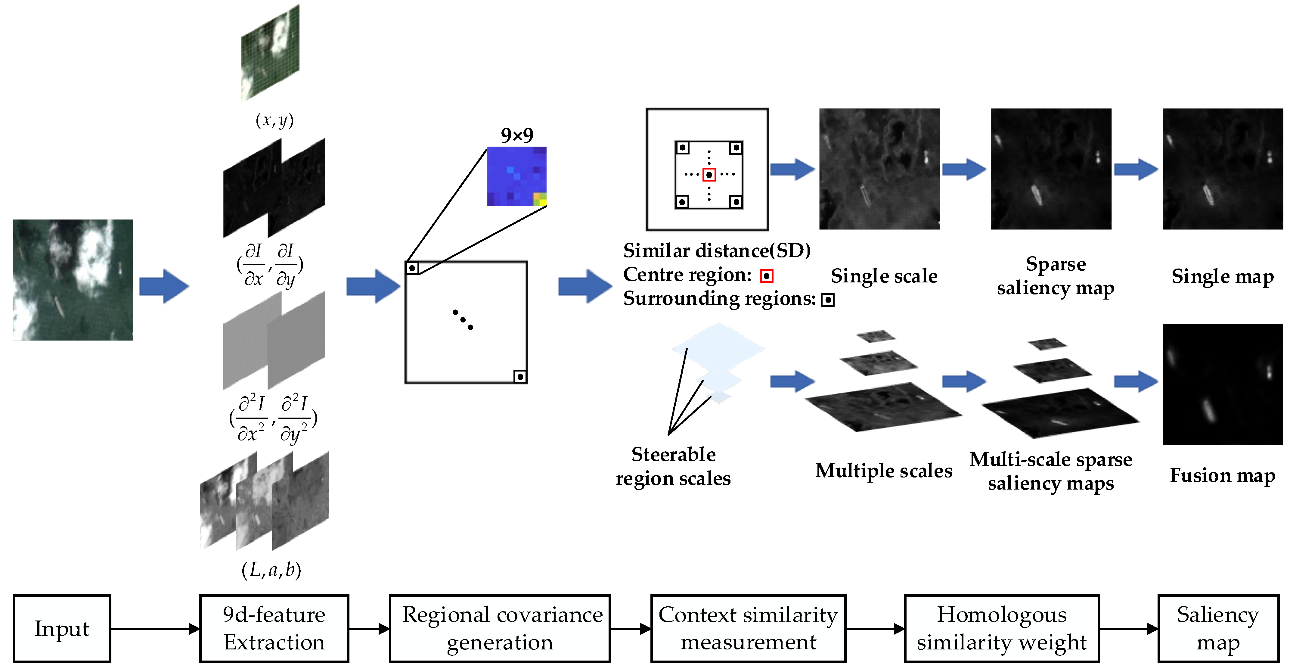
2.1. The Proposed Visual Saliency Model

The maritime background of ship detection in VRSIs mainly includes sea surface with great similarity, clouds with spatial randomness and chaos, and islands with color consistency. Additionally, the shapes of maritime ships have some characteristics, such as regularity, symmetry, and clear outlines, which make them become salient targets at sea. Synthetically, there are some obvious differences in color distinction, edge distribution, and structure information between the background and the ship target. To reflect the above differences, the statistical feature is considered to be an efficient description in the VRSIs. The regional covariance statistics feature used in our saliency model is a nonlinear descriptor, which can capture the local structure well on account of its statistical characteristics.

To illustrate the regional covariance statistics feature, consider the image given in Figure 2a. Perceptually, the covariance matrices that represent the region statistics feature are different in Figure 2b. In detail, firstly, the performance of regions of interest (ROIs), including patch I and patch VI, is significantly different from that of the patch II (cloud and fog), patch III (cloud and sea) and patch VI (sea). Secondly, patch IV and I as ROIs have the similar covariance matrix, even if the former is uniform and the latter is not. In other words, region covariance, as an ensemble statistical feature, can represent the complexity of the present region block. Based on this fact, we construct a new saliency model. In our work, we decompose the image into non-overlapping regions and then calculate the covariance feature of each region. Each image region (local neighborhood of a region) is compared against its immediate context described by the nearby regions, which gives a similarity distance (SD) value. Two regions with similar uniformity have similar covariance and give a smaller similarity distance value. Compared with SR Model [19] and CA Model [43], which are famous for suppressing background, our model performs better and ensures that ROIs are not corroded.

Next, we explain the proposed saliency model in detail as shown in Figure 3. There are three main steps. First, the region covariance feature is extracted by aggregating some simple features. Secondly, the SD method related to contextual comparison is used to quantify the regional saliency. Third, homologous similarity weighting is used to improve the contrast between the ROIs and the background. Finally, multi-scale fusion of saliency maps is designed to solve the scale problem.

In detail, given an H × W image, according to the regularity and clear outline of the ship targets, we extract the position coordinates and the intensity derivative. In addition, Lab color space, (dimension L, opposite color a and b), which is close to the human vision, is transformed from RGB color space. The nine-dimensional feature vectors for pixel m can be denoted as:

$$f_m=[x,y,L_m,a_m,b_m,\frac{\partial I}{\partial x},\frac{\partial I}{\partial y},\frac{{\partial }^{2}I}{\partial x^2},\frac{{\partial }^{2}I}{\partial y^2}]$$

(1)

where $\left(x,y\right)$ is the coordinate of pixel m, and the first derivative of the image intensity is calculated by the filter ${\left[-1,0,1\right]}^T$, and the second derivative is obtained by filtering again on the basis of the first derivative. To obtain the description of each region, the input image is firstly divided into non-overlapping square regions with a size of $n\times n$. For every region R, the feature of all pixels within the region can be aggregated by a 9-dimensional covariance:

$$C_R=\frac{1}{n^2-1}{\displaystyle \sum _{i=1}^{n^2}(f_i}-\mu ){(f_i-\mu )}^T$$

(2)

where ${\left\{f_i\right\}}_{i=1,2,\dots ,n^2}$ denotes the nine-dimensional features of all the pixel in region R, and $\mu$ represents the mean in region R.

Then, we obtain the covariance description through a fast calculation that uses the first and second-order integral image representations [44]. Obviously, Euclidean distance and the Mahalanobis distance cannot measure the similarity of covariance matrices, because the covariance matrix is not in Euclidean space. Inspired by the concept of sigma set [45], Cholesky decomposition is adopted to distinguish the two different distributions. It can be understood that each positive definite matrix can be factorized uniquely into the product of the lower triangular matrix L with its transpose, and the factorized matrix S consists of a set of points in Euclidean space, which is expressed as:

$$S=\left\{\begin{array}{cc}{L}_i\hfill & 1\le i\le k\\ -L_i\hfill & k+1\le i\le 2k\end{array}\right.$$

(3)

where k is the feature dimensional and L is obtained by the inverse calculation of Cholesky decomposition $C_R=L{L}^T$. Then, $L_i$ is the ith column of the low triangular matrix L. Using the set S given in Formula (3), a feature vector can be obtained by simply concatenating its elements. Moreover, the feature can be easily incorporated into this representation scheme by adding the mean vector of region R [46]. In this way, the enriched feature vector that can encode $C_R$ indirectly, is expressed as:

$${\psi }_{\mu }(C_R)=(\mu ,s_1,s_2,\dots ,s_k,,s_{k+1},.s_{k+2}..,s_{2k})$$

(4)

Then, we compare the similarity distance (SD) related to the context. As shown in Figure 3, assuming that the surrounding of R is a rectangular block within a radius of r, the rectangular block contains all local regions except for the central region R. Obviously, the surrounding region consists of ${\left(2r+1\right)}^2-1$ patches. Thus, the SD between region R and the ith surrounding patches is denoted as:

$$d(R,R_i)=\parallel {\psi }_R-{\psi }_{R_i}\parallel$$

(5)

where $i=1,2,\dots ,{\left(2r+1\right)}^2-1$. After ranking the SDs in ascending order, we use the first j values as the optimal similarity measure values. Then, the saliency of R is defined as the weighted average of the dissimilarities between region R to the T most similar regions around it. More formally, the saliency of region R is given by:

$$Sal={\displaystyle \sum _{j=1}^T{d}^j{}_{R,Ri}}$$

(6)

where $d_{ R,Ri}^j$ represents the jth optimal similarity distance value. The parameters in the model are set as T = 5, r = 3.

When calculating the similarity of the context regions, we find that in 9-dimensional features, the second-order derivative of intensity is beneficial to highlight edge features and had a good removal effect on chaotic clouds and fog. However, it also corroded prominent targets, resulting in low contrast and loss of prominent targets. Therefore, to enhance the contrast and obtain a sparse image containing the salient regions, the gaussian weight based on the unified kernel takes into account the surrounding region of central region R. We use the concept of homologous similarity [47] to construct the Gaussian weight function. This function, representing the probability of that covariance matrix belongs to the same background region, is given by a decreasing function of the distance:

$$w_j(R,R_i)=\exp (-\frac{1}{{\delta }_h}Dis{t}_{R,Ri})$$

(7)

where ${\delta }_h$ is the normalization parameter of the distance set $\left\{Dis{t}_{R,Ri}|i=1,2,\dots ,{\left(2r+1\right)}^2-1\right\}$ and represented as ${\delta }_h={\sum }_1^{{\left(2r+1\right)}^2-1}Dis{t}_{R,Ri}$. Based on a measure rule of regional covariance in [48], the SD is defined as:

$$Dis{t}_{R,Ri}=\sqrt{{\displaystyle \sum _{i=1}^n{\ln }^2{\lambda }_i(C_R,C_{Ri})}}$$

(8)

where ${\lambda }_i$ represents the ith generalized eigenvalue between $C_R$ and $C_{Ri}$. Combined with the above proposals, the saliency of region R is expressed by:

$$Sal={\displaystyle \sum _{j=1}^T{w}_j(R,R_i})d^j{}_{R,Ri}$$

(9)

Thus, the saliency map can be obtained by applying Formula (9) to all non-overlapping regions.

2.2. Multi-Scale Fusion of Saliency Maps

In the saliency model, the single-scale saliency map is based on the region covariance. Therefore, the size of the region affects the expression of the saliency. For the problem of scale variation, we design the steerable region scales in Figure 3 to guide the multi-scale fusion of saliency maps.

According to the single-scale saliency map generation process, we can extend it to the multi-scale maps. By adjusting the steerable region scales, in Figure 4, three scales of the saliency maps are generated and interpolated to obtain the new maps, which are of the same size as the input image. In this way, three single-scale saliency maps can be multiplied for fusing. After normalizing the fused map to [0, 256], the saliency value at the saliency map pixel x is denoted as:

$$S(x)=Nor({\displaystyle \prod _{\sigma \in \Gamma }Sa{l}_{\sigma }(x)})$$

(10)

where $\sigma$ represents normalized operation, $\prod \left(·\right)$represents the multiplicative fusion strategy, and$Sa{l}_{\sigma }\left(x\right)$ represents the score of the original map region R at the saliency map pixel x.

As shown in Figure 4b–d, on a coarse scale (Scale 1), it is beneficial to highlight the significant areas, while on a fine scale (Scale 2), the effect is better for cloud removal. In fact, as the size of the region increases, the feature representation ability of the region increases but the resolution of the saliency map decreases, which could miss the details. Therefore, multi-scale fusion is effective to keep a balance between regional descriptions and details. The fused saliency map in Figure 4e performs the best than the single-sale saliency. It does not matter if the background is chaotic, or if the size of the ship target is variable.

2.3. Candidate Target Extraction

After the fusion of the saliency maps, candidate regions can be obtained by the segmentation, which is a transitional step between the coarse detection and the fine detection. An appropriate threshold can accurately extract the candidate region and generate a small number of false alarms. Since the salient scores may vary widely across all regions of a map, we adopt a local threshold segmentation model [49] to generate adaptive thresholds for obtaining the binary graph. As shown in Figure 5, we have achieved the maximum segmentation quality for extracting the saliency regions.

3. Ship Target Identification

Saliency extraction guarantees a high recall. However, some false alarms, which are similar with the ship targets, are also mixed into the candidates, such as clutter, islands, and clouds. Therefore, we need to detect real ships and weed out the false alarms mentioned. Then, we design a ship identification framework, where an efficient feature descriptor combined with classifiers is used to achieve the detection requirements.

An efficient feature must not only accurately distinguish between targets and false alarms, but also keep unchanged for some changes to some image variations, especially the target rotation. As we all know, the histogram of oriented gradients (HOG) has been proven to be one of the best feature descriptors [21]. Although HOG can distinguish between true targets and false alarms, it performs poorly when coping with target rotation. As is shown in Figure 6, only if the rotation angle is an integer multiple of the bin size, HOG can be obtained by the circular shifts in Figure 6b,e. For other rotations, such as the presentation in Figure 6c,f, HOG could be calculated approximately and not rotationally invariant. Therefore, the study in [50] proposed Fourier HOG, which used Fourier analysis for HOG in the frequency domain. In the process, the former ideas, such as quantization angle and principal direction extraction, were abandoned. Instead, they extracted the rotation-invariant features directly from the candidate regions. Inspired by Fourier HOG, we construct a self-guided trigonometric kernel and partly extract the rotation-invariant feature as channel features to cope with the problem caused by the direction change.

Another problem, due to the similarity between the ship wake waves and the target edge in Figure 7, Fourier HOG performs poorly for this situation. To improve the discrimination of wake waves from the similar ships, we add an additional feature for further improvement. This improvement is necessary. As shown in Figure 7, the most prominent feature is the two parallel boundaries, which are very similar to some ship wake waves. Even so, the ship target is uniform to a great degree, while for the ship-like waves, the edge and interior show some differences. Therefore, we introduce the Circular Frequency (CF) filter [51] as another description. On the one hand, CF does not focus on image gradient, but the brightness changes between the overall area of the ship and the surrounding environment. On the other hand, the feature is extracted from the central circle of the ship, rather than adjacent pixels based on Fourier HOG. Therefore, CF can provide some distinguishing information as a supplementary to Fourier HOG.

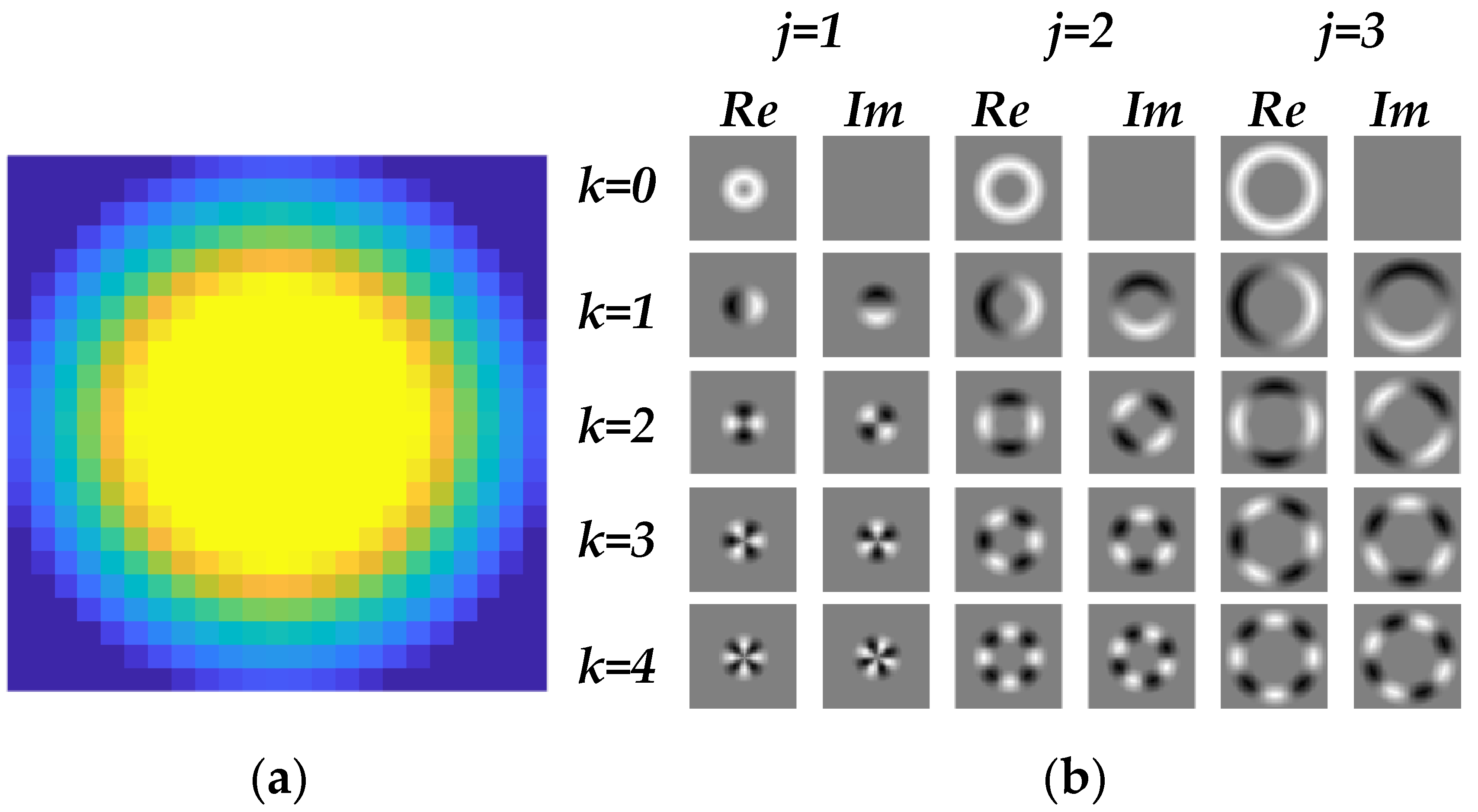
3.1. Fourier HOG Convolution Feature Generation

Fourier HOG uses a continuous representation in the gradient direction by creating an orientation distribution function h on each pixel. Let $D\left(x,y\right)$ and $\theta \left(D\left(x,y\right)\right)$ be the magnitude and the phase according to complex arithmetic. The continuous histogram of gradient direction can be regarded as a continuous impulse function curve with a direction period of $2\pi$:

$$h(\zeta )=‖D(x,y)‖\delta (\zeta -\theta (D(x,y)))$$

(11)

Therefore, the Fourier representation of the gradient distribution function $h\left(\zeta \right)$ can be expressed as:

$$h(\zeta )={\displaystyle \sum _{m=-\infty }^{\infty }{c}_m{e}^{im\zeta }}$$

(12)

where the coefficient $c_m=\langle d,e^{im\zeta }\rangle =\frac{1}{2\pi }{\int }_0^{2\pi }d\left(\zeta \right)e^{-im\zeta }d\zeta$, with $m\in Z$. Limiting the value of the maximum frequency order, m is equivalent to low-pass filtering in the frequency domain, which provides a “soft binning” smoothing effect. Thus, a series of complex coefficient images can be generated with the combination of Formulas (11) and (12):

$${\widehat{c}}_m(x,y)=\frac{1}{2\pi }{\displaystyle {\int }_0^{2\pi }h(\zeta )}{e}^{-im\zeta }=‖D(x,y)‖e^{-im\theta (D(x,y))}$$

(13)

where $m\in \left[0,M\right]$ and M is used to describe the maximum order of the image gradient. An example of this expansion is shown in Figure 8.

To generate the rotation-invariant feature, one measure is to analyze it in polar coordinates. The polar coordinate system can separate the angular part from the radial part, which is expressed as:

$$U(r,\phi )=P(r)\psi (\phi )$$

(14)

We only need take necessary measures to keep the angular part $\psi \left(\phi \right)$ unchanged because of the natural rotation invariance of the radial part P(r). Next, Fourier basis ${\psi }_m\left(\phi \right)=e^{im\phi }$ is used for the angle part. For simplicity, we set the center of the image as the origin of polar coordinates. We consider a basis function V using the same form as different-order complex Fourier coefficient images, which is expressed as follows:

$$V_{j,k}(r,\phi )=P_j(r)e^{ik\phi },j\in N,k\in Z$$

(15)

where k and j represent the rotation order of the basis function and the index of the convolution kernel with $j\in \left[0,J-1\right]$. Let R denote the largest radius of the basis function and J denote the number of different profiles, then a set of J profile is defined by:

$$P_j(r)=\min \left(\max \left(1-\frac{\left|r-j\sigma \right|}{\sigma },0\right),1\right),\sigma =\frac{R}{J}$$

(16)

As shown in Figure 9, a set of cyclic basis functions was created by using different scale profiles and Fourier series (J = 4, K = 4).

Next, by computing the convolution between the basis function $V_{j,k}$ and the Fourier coefficient ${\widehat{c}}_m\left(x,y\right)$, we can create the rotation-invariant feature by the following convolution computation:

$$F_{j,k,m}(x,y)=V_{j,k}(x,y)\ast {\widehat{c}}_m(x,y)$$

(17)

Thus, the convolution feature has an order with $\widehat{k}=k-m$. Additionally, the rotation-invariant feature is constructed and consists of the following two components. If $\widehat{k}=0$, the feature equivalent to a scalar function is rotation-invariant. Otherwise, if $\widehat{k}\ne 0$, the amplitude of the convolution result is rotation-invariant. In addition, another component of the rotation-invariant feature is obtained by coupling two different convolutional results. However, to improve computation speed, only the former two features are considered and applied to classification.

3.2. CF Feature Generation

Based on the proposed problem that gradient similarity between the ship wake waves and target edge, we introduce an additional feature named the circular frequency (CF) feature. In the square image obtained by the saliency extraction, the ship target will be brighter or darker in Figure 10a,d than the background near it. Therefore, we select a circle having four points of intersection with the ship, whose center is the center of the ship. It can produce four regular bright changes at the ship due to four points of intersection, while it produces random and chaotic changes in the wake waves.

In detail, taking Figure 10a as an example, gray value variation along this circle tends to be “bright-dark-bright-dark”. For Figure 10d, gray value variation along this circle tends to be “dark-bright-dark-bright”. In summary, as shown in Figure 10b,d, the gray value variation will have two peaks and two valleys, which is similar with the periodic trigonometric signal. It is conceivable that the gray value variation pattern of the wake clutter is random and chaotic. The value variation is effective and special for ships and can be used to generate the effective feature to distinguish wake clutter.

To embody the gray value variation, the discrete Fourier transform (DFT) of gray value needs to be calculated. Specifically, let $f_k\left(k=0,1,\dots ,N-1\right)$ represents the nth pixel value along the circle. Then, DFT at the pixel (i, j) is calculated by the following computation:

$$F_{(i,j)}=\frac{1}{N}\sqrt{{\left({\displaystyle \sum _{k=0}^{N-1}{f}_k\cos \frac{ck\pi }{N}}\right)}^2+{\left({\displaystyle \sum _{k=0}^{N-1}{f}_k\sin \frac{ck\pi }{N}}\right)}^2}$$

(18)

where N is the number of the sampling points along the circle and c represents the coefficient that determines the frequency of the sine and cosine functions in DFT. Every pixel in the image, except those near the boundaries, will produce output amplitude $F_{\left(i,j\right)}$. The amplitude can avoid phase interference of the input signal well. Since the circles on the ship are two-period signals, we selected c = 2 to acquire a stronger response of the ships, and the wake clutter parts will give a smaller response.

3.3. CF-Fourier HOG Channel Feature Classification

The extracted Fourier HOG and CF features (CF-Fourier HOG) will be fed into the classifier to identify the real target. Some candidate regions extracted from wide VRSIs may be small and fuzzy. Therefore, instead of the traditional detection framework, we introduce aggregate channel feature (ACF) [52] and fast feature pyramid generation (FFPG) [53]. In the training phase, the structure-refinement target by the ACF model is input to a libsvm classifier. In the testing phase, FFPG is used for feature collection, which guarantees a fast detection rate and low computational requirements.

All aggregate channel features come from CF and Fourier HOG. In our work, three channels are used, which are real-value features among Fourier HOG with $\widehat{k}=0$, the magnitude of complex features among Fourier HOG with $\widehat{k}\ne 0$, and the generated CF feature. Feature pyramid generation is a pooling operation essentially. As the number of pyramid layers increases, the feature is presented from fine to coarse, and the feature structure is gradually enhanced. However, due to the computationally intensive secondary sampling, the FFPG model performs well to speed up the calculation with almost no loss. It estimates the feature on any scale $d_i$ by the base scale $d_0$ and the scale factor ${\lambda }_i$:

$$F_{d_i}=F_{d_0}\cdot {(d_0/d_i)}^{-{\lambda }_i}$$

(19)

where $\left\{F_{d_i}\right\}$ represents feature maps on different scales. The scaling factor ${\lambda }_i$ is simply estimated by Formula (19) before training and testing. The combination of aggregate channel feature and fast pyramid feature estimation are used to correct the bias and variance of the trained classifier caused by various deformations (e.g., rotation and shift). Then, an identification framework shown in Figure 11 is proposed for the classification.

Note that features of a larger magnitude may affect the expression of some other important features. Therefore, we normalize the features and then feed them into the classifier.

4. Experiment Results

In this section, all the experiments are tested and evaluated on a computer with an Intel Core i9-10900 2.80 GHz CPU, 24 GB computer memory, and GeForce GTX 3070 GPU with 8 GB memory, and some deep learning models are implemented with the open-source Pytorch1.8 framework. First, we propose an VRS ship dataset. Second, our saliency method is compared with current excellent saliency models including subjective comparison and quantitative comparison. Third, we implement the rotation-invariance verification. Finally, the effectiveness of the overall detection framework is evaluated by comparing it with other commonly used and excellent methods.

4.1. VRS Ship Dataset

As far as we know, there are many public datasets for VRS ship detection. Based on the background of marine ship detection, we mainly introduce MWPU VHR-10 [54], HRSC2016 [55], MASATI [56], and Airbus Ship dataset [57], which have important influences in the field. The detailed differences between them and the VRS ship dataset are summarized in

Table 1. Comparison of different optical remote sensing datasets.

Dataset	Images	Class	Ship Instances	Image Size	Source
NWPU VHR-10	800	10	302	/	Google Earth
HRSC2016	1061	3	2976	300 × 300~1500 × 900	Google Earth
Airbus Ship dataset	192,570	2	/	768 × 768	Google Earth
MASATI	6212	7	7389	512 × 512	Aircraft
VRS ship dataset	893	6	1162	512 × 512	Google Earth

. Note that the image size in NWPU VHR-10 varies depending on their acquisition method.

The VRS ship dataset is collected from Google Earth. It contains 893 visible remote sensing images with a size of 512 × 512, whose spatial resolutions range from 2 to 15 m. The size of ship targets within the dataset ranges from about ten pixels to dozens of pixels. Each image has been manually labeled according to the following six classes: ship, multi, detail, ship with clouds, ship with sea waves, and background distractions. Since our method is based on small training samples, the method has a higher demand for the dataset. To meet this requirement, the different categories of the VRS dataset cover almost all marine backgrounds, such as thin clouds, fog, sea clutter, and island disturbances. Moreover, small and medium-sized ships under different lighting conditions are the main targets. To display the VRS ship dataset more intuitively, different classes of images are shown in Figure 12.

4.2. The Comparative Experiments of Saliency Extraction

4.2.1. Subjective Comparison

The representative saliency methods, which are classic and considered state of the art, are selected according to the following factors: a visual attention model (ITTI) based on cognitive psychology, neuroscience, and other disciplines [17]; a frequency domain model (SR) based on screening high and low frequency [19]; a computing model (CA) based on context awareness [43]; a statistical feature model (COV) based on integration of basic features [46]; a supervised saliency model (DRFI) based on local saliency-feature integration [58].

By the comparison in Figure 13, the proposed method is superior to most of the existing saliency models. In detail, it includes the following advantages:

• If multiple targets exist in a small range, our saliency result shows less aggregation phenomenon (in the first row of Figure 13), which is conducive to obtaining every target after the following threshold segmentation.
• If the contrast between the targets and the background is low, such as the presence of the thin cloud (in the second row of Figure 13), our method can guarantee the integrity of the target. In addition, if there is the interference from thick cloud (in the third row of Figure 13), our saliency method removes cloud interference further and is more effective.
• If there is interference such as the wake waves and the islands (in the fourth, fifth and sixth row of Figure 13), our saliency method performs best in comparison with all the above algorithms. In terms of the proposed model, not only can it remove most of the interference, but also is best in the edge weakening effect than other methods.

Moreover, CA and DRFI have great advantages in the salience of the ship targets. However, when the thick cloud gives strong interference, the background cannot be suppressed well. Although SR can suppress the background better, it causes the loss of the background-like ship targets. ITTI does not perform well at capturing the artificial targets, especially the ship target. DRFI and COV represent the peak of current ship saliency detection. Explicitly, the multi-scale module in the COV model brings unnecessary computation, while it could not highlight real targets stably. As for the DRFI model, it mainly considers the regional contrast and background features. However, due to the response of the background area, high saliency values are assigned to the clump of clouds in the background (in the fourth row of Figure 13), which burdens the identification stage.

4.2.2. Quantitative Comparison

Then, we use the receiver operating characteristic (ROC) curve and the area under the curve (AUC) to quantitatively evaluate the saliency model. To draw the ROC curve, one hundred images are firstly tested to obtain the corresponding saliency maps. Then, we normalize all the saliency maps to [0, 255]. Therefore, 256 masks are generated with a threshold sliding from 0 to 255. Finally, the true positive rate (TPR) and the false positive rate (FPR) as two variables of ROC curve are computed with respect to the ground-truth, which are expressed as:

$$TPR=\frac{TPs}{Ps}$$

(20)

$$FPR=\frac{FPs}{Ns}$$

(21)

where TPs represents the numbers of all pixels that are counted as true and whose value exceeds the mask threshold, Ps represents the numbers of all the true pixels in the ground truth, FPs represents the numbers of all pixels that are counted as false and whose value does not exceed the mask threshold, and Ns represents the numbers of all the false pixels in the ground truth.

As shown in Figure 14, the closer the ROC curve is to the upper left corner, the better the detection performance of the model will be. In other words, the AUC value is larger. The blue curve in Figure 14a represents the proposed saliency model, which is closest to the upper left corner. The corresponding AUC value in Figure 14b is also the largest. Combined with subjective and objective evaluation analysis, the proposed saliency model has certain validity and reliability in the extraction of the candidate ships.

4.3. Rotation-Invariant Channels Verification

To ensure robustness to target rotation, low-level rotation invariance is necessary. Hence, we design a confirmatory experiment to verify the efficiency of the rotation-invariance channel features. Since all the rotation-invariant channel features come from Fourier HOG, we directly verify the extracted Fourier HOG with a self-guided trigonometric kernel in Figure 9.

In detail, we visualize the Fourier HOG in twelve directions. For each candidate region with a size of 56$\times$56 in Figure 15a, the target orientation varies by 30 degrees clockwise. Considering the parameters $K=4, M=4,J=4$ in Formulas (13) and (16), the features almost have the same response in different directions in Figure 15b.

4.4. Overall Detection Performance and Comparison

After completing the entire process of ship detection, we conduct the comparative experiments. To obtain an optimal experimental result, some preparations are carried out before the comparison, which includes several important modules, such as candidate region setup, feature extraction, feature pyramid, classifier setup, and so on. Finally, the evaluation and detection results are given for analyzing some details of our proposed method.

4.4.1. Preparations

In the candidate region setup, we adjust the size of the candidate regions. According to the result of saliency extraction, the size of candidates is not square. However, square maps facilitate the extraction of feature pyramids. Therefore, for the convenience of the experiment, all candidate regions are adjusted into squares with 56 $\times$ 56 as shown in Figure 16. Thus, there are two types of samples in all candidate regions used for the classifier training and testing. One type includes real ship targets as positive samples, and the other includes some false alarms as negative samples.

In the feature extraction, we give some parameter settings. As mentioned earlier, all the channel features used in our case mainly consist of three parts. Specifically, for the former two-channel features, three parameters need to be considered, namely, the rotation order (k) of convolutional kernels, the maximum radius (r) of convolutional kernels and the number of Fourier order (m). We assign five radius scales to the value of r, i.e., $r\in \left\{0,6,12,18,24\right\}$, while m is set to 1, 2, 3, and 4 as suggested in [50].

For the latter channel features, as shown in Figure 11, we choose the 16 × 16 subimage in the upper left corner of the CF-filtered image as the first block. It is separated into four subblocks named the cells. For each cell, we get a 9-D histogram from the CF-filtered image. Then, the histograms from the four cells are combined and normalized by the energy density of the block, and the outcome is the 4 × 9 = 72-dimensional feature representations of this block. The block is set to traverse the entire image with the step of 64 pixels. For each step, we can obtain a 72-dimensional feature vector. Finally, the combination of these feature vectors forms the final CF feature of (7 − 1) × (7 − 1) × 72 = 1152-dimensional.

In the feature pyramid module, we sample the image at a sampling rate of 1/2 on four different scales ($1,2^{-1},2^{-2},2^{-3}$) to estimate the scale factors. Thus, the FFPG model can compute pyramid features faster.

In the classifier setup, we use linear lib-SVM to train the classifier, and the proportion of positive and negative samples is 1:4. Note that some of the negative samples used in the training and testing phases are derived from candidate regions, and the other part is selected by using the sliding window and coarse sample image pyramids. Finally, 80% of the sample is designated as the training set and the rest as the test set.

4.4.2. Comparison of Overall Detection Performance

To verify the effectiveness of our proposed method, we conduct some experiments among the current popular target detectors. The metrics of recall/precision rate, F1-score, and average precision (AP) are used to assess the precision, and running time is used to assess the detection speed. To be more specific, when the intersection ratio (IoU) between the detection bounding box and the ground truth box exceeds 50%, it is counted as true (TP); otherwise, it is false negative (FN). Let the false alarm that is classified as true target record as FP. Therefore, the precision/recall rate are calculated with the following formulas:

$$Precision=\frac{TP}{TP+FP}$$

(22)

$$Recall=\frac{TP}{TP+FN}$$

(23)

$$F1=2\times \frac{Precision\times Recall}{Precision+Recall}$$

(24)

Average Precision (AP) calculates the average accuracy of recall values from 0 to 1. That is, AP is the area bounded by the PR curve and the coordinate axes. Let r represents recall rate and P (r) represents accuracy rate corresponding to the curve. Then, we can calculate AP:

$$AP={\displaystyle {\int }_0^{1}P(r)dr}$$

(25)

To quantitatively evaluate the above performances, our comparative experiments, which contain several state-of-the-art methods, could be roughly divided into three parts. For the first part, to verify the effect of the proposed CF-Fourier HOG channel features, the methods based on HOG and Fourier HOG feature are conducted to make a comparison. To ensure fairness, our candidate region extraction process is applied to the practice of HOG and Fourier HOG. For the second part, we compare with an excellent “coarse to fine” ship detection method [24]. In the third part, we supplement several advanced and effective deep learning detection models, including Yolov3 [29], Yolov4 [32], Faster R-CNN [36], CenterNet [59], SSD [60], and Yolov5 Series, which are increasingly improved and applied to ship detection. All the deep learning models are trained for 200 epochs and obtain the optimal weights. Then,

Table 2. The performance comparison of different methods on VRS ship dataset.

Methods	Backbone	Recall	Precision	F1	[email protected]	[email protected]	[email protected]:0.95	Running Time (s)
HOG	/	78.89%	46.11%	0.58	71.89%	/	/	0.4852
SSD	VGG-16	84.88%	79.58%	0.82	86.69%	66.20%	53.63%	0.0089
	MobileNetv2	89.19%	80.69%	0.85	87.02%	57.03%	52.81%	0.0083
Method in [24]	/	90.16%	88.24%	0.89	87.25%	/	/	0.2248
Yolov3	DarkNet-53	92.67%	90.09%	0.91	90.04%	21.37%	37.91%	0.0154
Fourier HOG	/	89.84%	94.12%	0.92	91.47%	64.56%	59.28%	1.3954
Faster R-CNN	ResNet-50	84.57%	92.49%	0.88	91.61%	52.50%	50.14%	0.0556
	EfficientNet	88.34%	91.59%	0.93	92.05%	62.17%	58.39%	0.0439
CenterNet	ResNet-50	94.33%	91.45%	0.93	92.34%	76.38%	65.42%	0.0125
Yolov4	CSPDarknet53	92.79%	86.31%	0.89	91.55%	39.51%	46.27%	0.0206
Yolov5-Nano	CSPDarknet53	90.69%	95.27%	0.93	90.44%	66.63%	57.84%	0.0124
Yolov5s	CSPDarknet53	93.89%	95.76%	0.95	94.61%	74.47%	63.16%	0.0125
Yolov5m	CSPDarknet53	92.79%	95.17%	0.94	94.22%	76.43%	64.70%	0.0161
Yolov5l	CSPDarkNet53	93.62%	92.22%	0.93	94.32%	79.03%	66.15%	0.0252
Yolov5x	CSPDarknet53	95.10%	93.37%	0.94	95.70%	80.30%	68.10%	0.0390
Proposed Method	/	94.27%	92.73%	0.93	94.46%	77.99%	65.37%	0.1162

lists the quantitative results of all the assessments.

Although the results of deep learning methods are generally good, especially running time, as a whole the proposed method has better detection performance. According to Table 2, we can draw the following conclusions:

First, the method based on the HOG, which ignores the rotation behavior of the ship target, results in the worst performance. Method [24] has solved the rotation problem and given a higher precision and recall. Same as our method, they both use the “coarse-to-fine” detection scheme. However, our proposed method gives the best results in all metrics.

Second, compared with the method based on Fourier HOG, the proposed method improves the recall rate by 4.43%. However, for a faster detection speed, the proposed channel features discard a part of the original Fourier HOG, which results in a 1.39% reduction in precision rate. Nevertheless, the improvement greatly reduces the overall detection time.

Third, the deep learning network can extract some semantic information, which helps to locate the target accurately. Therefore, the recall rate is generally high, but for the ship target recognition, the detection accuracy varies greatly. SSD gives a lower detection accuracy. In the Faster-RCNN experiment, not only the anchors are complicated, but also the detection speed is slow. Even though the newer network backbone named MobileNet v2 [61] is used to replace the original backbone of SSD, the metrics are still unsatisfactory. Contrastingly, instead of ResNet, EfficientNet [62] is used in the Faster-RCNN model, which obtains acceptable results. Since the complex and the inefficient anchors are removed, CenterNet has a great improvement in running time without losing accuracy. Yolov4 and Yolov5 Series give better results, which can accurately locate ships and remove false alarms. Although these methods have a faster detection speed, the proposed method outperforms most methods in terms of AP metric. In addition, our method does not rely on large amounts of training data and dedicated computing platforms such as GPUs, which is more suitable for UAVs.

Finally, for a more comprehensive comparison, Figure 17 is expanded to contain the detection results of various situations, such as small-sized ships, medium-sized ships, multi-target aggregation, sea clutter, wake waves, and cloud interference. In addition, some detection results using the proposed method on the MASATI dataset and VRS ship dataset are shown in Figure 18.

5. Discussion

In this work, we summarize several challenges for maritime ship detection and propose the VRS ship dataset. Then, mainly focusing on the problems of the target scale, the target rotation, and various backgrounds, we propose a “coarse to fine” detection scheme. It provides a simple and easy idea to apply to the detection based on small training samples.

In the candidate region extraction stage, we propose a saliency model specially designed to quickly highlight the potential ship targets. The subjective experiment in Figure 13 shows that the model does a good job of suppressing background and reducing contour erosion. Based on this advantage, it can not only be used for the extraction of potential ships at sea, but also can be extended to other fields, such as industrial crack detection. Then, we conduct a multi-scale fusion process to overcome the problem of scale variations. Instead of an inefficient down-sampling process, the steerable region scales are designed to generate saliency maps on multiple scales. Compared with several state-of-the-art saliency models, the fused saliency model gives the highest AUC of 0.9476, which implies a better performance for the localization of potential ships.

In the ship identification stage, inspired by aggregate channel features, we design a three-channel feature for arbitrary-orientation target recognition and a new framework that combines fast feature pyramids to improve detection speed. Compared with Fourier HOG, the proposed method reduces the feature dimension and results in a 1.39% reduction in accuracy rate. Nevertheless, this tiny precision sacrifice makes sense, which F1 and [email protected]:0.95 improved by 0.02 and 6.09%, respectively. Additionally, the improvement reduces the overall detection time. Experiment results indicate that the overall detection achieves the better performance of 65.37% and 0.1162 s in terms of [email protected]:0.95 and running time, which basically meets the need of the near-real-time tasks.

The main work of deep learning is not to design the feature engineering, but to mine potential features based on data to improve the robustness of detection. Yolov5x and Yolov5s have better detection performance in terms of AP and F1, as well as higher accuracy values. In the case of cloud interference and multi-target aggregation, their results are better with fewer misdetections than the proposed method. However, as shown in Figure 17 (the third row), when the small and medium-sized ships appear in the same image by accident, the detection of small targets is poor. It can be said that having fewer data is not enough to learn more efficient features in these data-driven models. On the contrary, our method does better in this case. Since the different scales of sparse targets have little effect on the competition for local-region saliency in the saliency model, more comprehensive potential targets of different scales can be extracted for classification. Therefore, it is meaningful of the proposed method to meet the needs of small sample dataset detection. Further, benefiting from saliency extraction and feature design, the proposed method gains excellent results.

Detection results on MASATI and the VRS ship dataset show that, in most cases, the proposed method can accurately locate the position of the ship targets, even though the target within the MASATI is smaller. Moreover, the proposed VRS ship dataset focuses more on the practical complexities instead of the ideal case with less interference. Objectively speaking, there are also some misdetections and missed detections. The failure results are discussed as follows. For the target misdetections, a small number of clouds, similar to the white ships, may lead to false alarms being misidentified as targets with small confidence values. For missed detection, on the one hand, due to the low illumination and the particularity of the ship’s coating, the color of the ship’s hull is close to the color of the sea surface. On the other hand, issues such as cloud occlusion and RSI clipping may be bad for capturing the ship features, leading to missed detections in Figure 18.

From the application perspective, the VRS ship dataset is obtained from Google Earth. Maybe for some special occasions, Google Earth does not provide high-resolution images, which is a limitation. For other ship datasets, such as the MASATI collected by aircraft, high-resolution images are also available. The experiments in Figure 18 show that our method still has better detection results on the MASATI dataset. In addition, the trained model of the proposed method is smaller and more efficient, which can be well embedded into chips. Despite a few misdetections and missed detections mentioned above, our work is still meaningful for the small UAV platform.

6. Conclusions

Ship target detection in VRSI is a challenging problem due to the various backgrounds and variations in ship scale and orientation. In this paper, we propose a “coarse to fine” detection method based on the small training samples. Experiments show that the proposed model has excellent performance. The proposed saliency model has a positive significance for locating the target quickly. Additionally, the modified channel features have a lower dimensionality and a stronger description ability insusceptible to the target’s rotational behavior. However, to enhance the practicality of the model, improving the detection speed is still an important research direction.

Our future work will focus on two aspects. First, we will build a rotating ship dataset containing thousands of optical remote sensing images. The proposed dataset in the paper is quite practical; however, it does not have rotation annotations, which is not conducive to detecting the primary orientation of the target. Second, more efficient convolutional channel features and feature fusion can be further explored to improve the detection speed with tiny precision sacrifice.

References

1. Li, J.; Tian, J.; Gao, P.; Li, L. Ship Detection and Fine-Grained Recognition in Large-Format Remote Sensing Images Based on Convolutional Neural Network. In Proceedings of the IEEE International Geoscience and Remote Sensing Symposium (IGARSS), Waikoloa, HI, USA, 26 September–2 October 2020. [Google Scholar]
2. Lei, Y.; Leng, X.; Ji, K. Marine Ship Target Detection in SAR Image Based on Google Earth Engine. In Proceedings of the IEEE International Geoscience and Remote Sensing Symposium (IGARSS), Brussels, Belgium, 11–16 July 2021. [Google Scholar]
3. Zhang, R.; Su, Y.; Li, Y.; Zhang, L.; Feng, J. Infrared and Visible Image Fusion Methods for Unmanned Surface Vessels with Marine Applications. J. Mar. Sci. Eng. 2022, 10, 588. [Google Scholar] [CrossRef]
4. Cheng, G.; Han, J. A Survey on Object Detection in Optical Remote Sensing Images. ISPRS J. Photogramm. Remote Sens. 2016, 117, 11–28. [Google Scholar] [CrossRef] [Green Version]
5. Harvey, N.; Porter, R.; Theiler, J. Ship Detection in Satellite Imagery Using Rank-Order Grayscale Hit-or-Miss Transforms. In Proceedings of the Conference on Visual Information Processing XIX, Orlando, FL, USA, 6–7 April 2010. [Google Scholar]
6. Wang, S.; Stahl, J.; Bailey, A.; Dropps, M. Global Detection of Salient Convex Boundaries. Int. J. Comput. Vis. 2007, 71, 337–359. [Google Scholar] [CrossRef]
7. Yan, H. Aircraft Detection in Remote Sensing Images Using Centre-Based Proposal Regions and Invariant Features. Remote Sens. Lett. 2020, 11, 787–796. [Google Scholar] [CrossRef]
8. Shi, Z.; Yu, X.; Jiang, Z.; Li, B. Ship Detection in High-Resolution Optical Imagery Based on Anomaly Detector and Local Shape Feature. IEEE Trans. Geosci. Remote Sens. 2014, 52, 4511–4523. [Google Scholar]
9. Tang, J.; Deng, C.; Huang, G.; Zhao, B. Compressed-Domain Ship Detection on Spaceborne Optical Image Using Deep Neural Network and Extreme Learning Machine. IEEE Trans. Geosci. Remote Sens. 2015, 53, 1174–1185. [Google Scholar] [CrossRef]
10. Zou, Z.; Shi, Z. Ship Detection in Spaceborne Optical Image with SVD Networks. IEEE Trans. Geosci. Remote Sens. 2016, 54, 5832–5845. [Google Scholar] [CrossRef]
11. Xu, F.; Liu, J.; Sun, M.; Zeng, D.; Wang, X. A Hierarchical Maritime Target Detection Method for Optical Remote Sensing Imagery. Remote Sens. 2017, 9, 280. [Google Scholar] [CrossRef] [Green Version]
12. Nie, T.; Han, X.; He, B.; Li, X.; Liu, H.; Bi, G. Ship Detection in Panchromatic Optical Remote Sensing Images Based on Visual Saliency and Multi-Dimensional Feature Description. Remote Sens. 2020, 12, 152. [Google Scholar] [CrossRef] [Green Version]
13. Li, B.; Xie, X.; Wei, X.; Tang, W. Ship Detection and Classification from Optical Remote Sensing Images: A survey. Chin. J. Aeronaut. 2021, 34, 145–163. [Google Scholar] [CrossRef]
14. Zhou, H.T.; Zhuang, Y.; Chen, L.; Shi, H. Signal and Information Processing, Networking and Computers, 3rd ed.; Springer: Singapore, 2018; pp. 164–171. [Google Scholar]
15. Uijlings, J.; van de Sande, K.; Gevers, T.; Smeulders, A. Selective Search for Object Recognition. Int. J. Comput. Vis. 2013, 104, 154–171. [Google Scholar] [CrossRef] [Green Version]
16. Zhang, S.; Xie, M. Beyond Sliding Windows: Object Detection Based on Hierarchical Segmentation Model. In Proceedings of the International Conference on Communications, Circuits and Systems (ICCCAS), Chengdu, China, 15–17 November 2013. [Google Scholar]
17. Itti, L.; Koch, C.; Niebur, E. A Model of Saliency-Based Visual Attention for Rapid Scene Analysis. IEEE Trans. Pattern Anal. Mach. Intell. 1998, 20, 1254–1259. [Google Scholar] [CrossRef] [Green Version]
18. Achanta, R.; Estrada, F.; Wils, P.; Silsstrunk, S. Salient Region Detection and Segmentation. In Proceedings of the International Conference on Computer Vision Systems (ICVS), Santorini, Greece, 12–15 May 2008. [Google Scholar]
19. Hou, X.; Zhang, L. Saliency detection: A Spectral Residual Approach. In Proceedings of the IEEE Conference on Computer Vision and Pattern Recognition (CVPR), Minneapolis, MN, USA, 17–22 June 2007. [Google Scholar]
20. Ojala, T.; Pietikainen, M.; Maenpaa, T. Multiresolution Gray-Scale and Rotation Invariant Texture Classification with Local Binary Patterns. IEEE Trans. Pattern Anal. Mach. Intell. 2002, 24, 971–987. [Google Scholar] [CrossRef]
21. Dalal, N.; Triggs, B. Histograms of Oriented Gradients for Human Detection. In Proceedings of the IEEE Conference on Computer Vision and Pattern Recognition (CVPR), San Diego, CA, USA, 20–25 June 2005. [Google Scholar]
22. Yang, F.; Xu, Q.; Gao, F.; Hu, L. Ship Detection from Optical Satellite Images Based on Visual Search Mechanism. In Proceedings of the IEEE International Geoscience and Remote Sensing Symposium (IGARSS), Milan, Italy, 26–31 July 2015. [Google Scholar]
23. Yang, F.; Xu, Q.; Li, B.; Ji, Y. Ship Detection from Thermal Remote Sensing Imagery through Region-Based Deep Forest. IEEE Geosci. Remote. Sens. Lett. 2018, 15, 449–453. [Google Scholar] [CrossRef]
24. Dong, C.; Liu, J.; Xu, F. Ship Detection in Optical Remote Sensing Images Based on Saliency and A Rotation-Invariant Descriptor. Remote Sens. 2018, 10, 400. [Google Scholar] [CrossRef] [Green Version]
25. Wu, X.; Hong, D.; Tian, J.; Chanussot, J.; Li, W.; Tao, R. ORSIm Detector: A Novel Object Detection Framework in Optical Remote Sensing Imagery Using Spatial-Frequency Channel Features. IEEE Trans. Geosci. Remote Sens. 2019, 57, 5146–5158. [Google Scholar] [CrossRef] [Green Version]
26. Liu, W.; Ma, L.; Chen, H. Arbitrary-Oriented Ship Detection Framework in Optical Remote-Sensing Images. IEEE Geosci. Remote. Sens. Lett. 2018, 15, 937–941. [Google Scholar] [CrossRef]
27. Redmon, J.; Farhadi, A. YOLO9000: Better, Faster, Stronger. In Proceedings of the IEEE/CVF Conference on Computer Vision and Pattern Recognition (CVPR), Honolulu, HI, USA, 21–26 July 2017. [Google Scholar]
28. Hong, Z.; Yang, T.; Tong, X.; Zhang, Y.; Jiang, S.; Zhou, R.; Han, Y.; Wang, J.; Yang, S.; Liu, S. Multi-Scale Ship Detection from SAR and Optical Imagery Via a More Accurate YOLOv3. IEEE J. Sel. Top Appl Earth Obs. Remote Sens. 2021, 14, 6083–6101. [Google Scholar] [CrossRef]
29. Redmon, J.; Farhadi, A. YOLOv3: An Incremental Improvement. arXiv 2020, arXiv:1804.02767. [Google Scholar]
30. Wang, C.; Liao, H.; Wu, Y.; Chen, P.; Hsieh, J.; Yeh, I. CSPNet: A New Backbone that can Enhance Learning Capability of CNN. In Proceedings of the IEEE/CVF Conference on Computer Vision and Pattern Recognition (CVPR), Seattle, WA, USA, 14–19 June 2020. [Google Scholar]
31. He, K.; Zhang, X.; Ren, S.; Sun, J. Deep Residual Learning for Image Recognition. In Proceedings of the IEEE Conference on Computer Vision and Pattern Recognition (CVPR), Las Vegas, NV, USA, 27–30 June 2016. [Google Scholar]
32. Bochkovskiy, A.; Wang, C.; Liao, H. YOLOv4: Optimal Speed and Accuracy of Object Detection. arXiv 2020, arXiv:2004.10934v1. [Google Scholar]
33. Li, H.; Xiong, P.; An, J.; Wang, L. Pyramid Attention Network for Semantic Segmentation. arXiv 2018, arXiv:1805.10180. [Google Scholar]
34. Lin, T.Y.; Dollar, P.; Girshick, R.; He, K.; Hariharan, B.; Belongie, S. Feature Pyramid Networks for Object Detection. In Proceedings of the IEEE/CVF Conference on Computer Vision and Pattern Recognition (CVPR), Honolulu, HI, USA, 21–26 June 2017. [Google Scholar]
35. Wang, C.; Bochkovskiy, A.; Liao, H. Scaled-YOLOv4: Scaling Cross Stage Partial Network. In Proceedings of the IEEE/CVF Conference on Computer Vision and Pattern Recognition (CVPR), Nashville, TN, USA, 20–25 June 2021. [Google Scholar]
36. Shi, Q.; Li, W.; Tao, R.; Sun, X.; Gao, L. Ship Classification Based on Multi-feature Ensemble with Convolutional Neural Network. Remote Sens. 2019, 11, 419. [Google Scholar] [CrossRef] [Green Version]
37. Wang, N.; Li, B.; Wei, X.; Wang, Y.; Yan, H. Ship Detection in Spaceborne Infrared Image Based on Lightweight CNN and Multisource Feature Cascade Decision. IEEE Trans Geosci. Remote Sens. 2021, 59, 4324–4339. [Google Scholar] [CrossRef]
38. You, Y.; Cao, J.; Zhang, Y.; Liu, F.; Zhou, W. Nearshore Ship Detection on High-Resolution Remote Sensing Image via Scene-Mask R-CNN. IEEE Access 2019, 7, 128431–128444. [Google Scholar] [CrossRef]
39. Ren, S.; He, K.; Girshick, R.; Sun, J. Faster R-CNN: Towards Real-Time Object Detection with Region Proposal Networks. IEEE Trans. Pattern Anal. Mach. Intell. 2017, 39, 1137–1149. [Google Scholar] [CrossRef] [PubMed] [Green Version]
40. Lin, H.; Shi, Z.; Zou, Z.X. Fully Convolutional Network with Task Partitioning for Inshore Ship Detection in Optical Remote Sensing Images. IEEE Geosci. Remote. Sens. Lett. 2017, 14, 1665–1669. [Google Scholar] [CrossRef]
41. Dai, J.; Li, Y.; He, K.; Sun, J. R-FCN: Object Detection via Region-based Fully Convolutional Networks. In Proceedings of the International Conference on Neural Information Processing Systems (NIPS), Barcelona, Spain, 5–10 December 2016. [Google Scholar]
42. Liu, B.; Wu, H.; Su, W.; Zhang, W.; Sun, J. Rotation-Invariant Object Detection Using Sector-ring HOG and Boosted Random Ferns. Vis. Comput. 2018, 34, 707–719. [Google Scholar] [CrossRef]
43. Goferman, S.; Zelnik-Manor, L.; Tal, A. Context-Aware Saliency Detection. IEEE Trans. Pattern Anal. Mach. Intell. 2012, 34, 1915–1926. [Google Scholar] [CrossRef] [Green Version]
44. Viola, P.; Jones, M. Rapid Object Detection Using a Boosted Cascade of Simple Features. In Proceedings of the IEEE Conference on Computer Vision and Pattern Recognition (CVPR), Kauai, HI, USA, 8–14 December 2001. [Google Scholar]
45. Hong, X.; Chang, H.; Shan, S.; Chen, X.; Gao, W. Sigma Set: A Small Second Order Statistical Region Descriptor. In Proceedings of the IEEE Computer Society Conference on Computer Vision and Pattern Recognition Workshops (CVPR), Miami, FL, USA, 20–25 June 2009. [Google Scholar]
46. Erdem, E.; Erdem, A. Visual Saliency Estimation by Nonlinearly Integrating Features Using Region Covariances. J. Vis. 2013, 13, 11. [Google Scholar] [CrossRef]
47. Chen, Z.; Wang, H.; Zhang, L.; Yan, Y.; Liao, H. Visual Saliency Detection Based on Homology Similarity and An Experimental Evaluation. J. Vis. Commun. Image Represent. 2016, 40, 251–264. [Google Scholar] [CrossRef]
48. Tuzel, O.; Porikli, F.; Meer, P. Region Covariance: A Fast Descriptor for Detection and Classification. In Proceedings of the European Conference on Computer Vision (ECCV), Graz, Austria, 7–13 May 2006. [Google Scholar]
49. Peuwnuan, K.; Woraratpanya, K.; Pasupa, K. Modified Adaptive Thresholding Using Integral Image. In Proceedings of the International Joint Conference on Computer Science and Software Engineering (JCSSE), Khon Kaen, Thailand, 13–15 July 2016. [Google Scholar]
50. Liu, K.; Skibbe, H.; Schmidt, T.; Blein, T.; Palme, K.; Brox, T.; Ronneberger, O. Rotation-Invariant HOG Descriptors Using Fourier Analysis in Polar and Spherical Coordinates. Int. J. Comput. Vis. 2014, 106, 342–364. [Google Scholar] [CrossRef]
51. Kawato, S.; Tetsutani, N. Circle-Frequency Filter and Its Application. Ieice Tech. Rep. Image Eng. 2001, 100, 49–54. [Google Scholar]
52. Yang, B.; Yan, J.; Lei, Z.; Li, S. Aggregate Channel Features for Multi-view Face Detection. In Proceedings of the IEEE/IAPR International Joint Conference on Biometrics (IJCB), Clearwater, FL, USA, 29 September–2 October 2014. [Google Scholar]
53. Dollar, P.; Appel, R.; Belongie, S.; Perona, P. Fast Feature Pyramids for Object Detection. IEEE Trans. Pattern Anal. Mach. Intell. 2014, 36, 1532–1545. [Google Scholar] [CrossRef] [PubMed] [Green Version]
54. Cheng, G.; Han, J.; Zhou, P.; Guo, L. Multi-Class Geospatial Object Detection and Geographic Image Classification Based on Collection of Part Detectors. ISPRS J. Photogramm. Remote Sens. 2014, 98, 119–132. [Google Scholar] [CrossRef]
55. Liu, Z.; Yuan, L.; Weng, L.; Yang, Y. A High Resolution Optical Satellite Image Dataset for Ship Recognition and Some New Baselines. In Proceedings of the International Conference on Pattern Recognition Applications and Methods (ICPRAM), Porto, Portugal, 24–26 February 2017. [Google Scholar]
56. Gallego, A.J.; Pertusa, A.; Gil, P. Automatic Ship Classification from Optical Aerial Images with Convolutional Neural Networks. Remote Sens. 2018, 10, 4. [Google Scholar] [CrossRef] [Green Version]
57. Al-Saad, M.; Aburaed, N.; Panthakkan, A.; Al Mansoori, S.; Al Ahmad, H.; Marshall, S. Airbus Ship Detection from Satellite Imagery using Frequency Domain Learning. In Proceedings of the Conference on Image and Signal Processing for Remote Sensing XXVII, Electric Network, online, 13–17 September 2021. [Google Scholar]
58. Jiang, H.; Wang, J.; Yuan, Z.; Wu, Y.; Zheng, N.; Li, S. Salient Object Detection: A Discriminative Regional Feature Integration Approach. In Proceedings of the IEEE Conference on Computer Vision and Pattern Recognition (CVPR), Portland, OR, USA, 23–28 June 2013. [Google Scholar]
59. Zhou, X.; Wang, D.; Krhenbühl, P. Objects as Points. arXiv 2019, arXiv:1904.07850. [Google Scholar]
60. Liu, W.; Anguelov, D.; Erhan, D.; Szegedy, C.; Reed, S.; Fu, C.; Berg, A. SSD: Single Shot MultiBox Detector. In Proceedings of the European Conference on Computer Vision (ECCV), Amsterdam, The Netherlands, 8–16 October 2016. [Google Scholar]
61. Sandler, M.; Howard, A.; Zhu, M.; Zhmoginov, A.; Chen, L. MobileNetV2: Inverted Residuals and Linear Bottlenecks. In Proceedings of the IEEE/CVF Conference on Computer Vision and Pattern Recognition (CVPR), Salt Lake City, UT, USA, 18–23 June 2018. [Google Scholar]
62. Tan, M.; Le, Q. EfficientNet: Rethinking Model Scaling for Convolutional Neural Networks. In Proceedings of the International Conference on Machine Learning (ICML), Long Beach, CA, USA, 9–15 June 2019. [Google Scholar]
Figure 1. The flowchart of the proposed ship detection scheme.
Remotesensing 14 03347 g001
Figure 2. Saliency model based on regional covariance analysis. (a) The input remote sensing image. (b) Covariance matrixes of different patches. By using our context similarity measurement, the smaller the similarity distance (SD) is, the more similar the selected patches are. The SDs among different patches are d (I,II) = 12.98, d (I,III) = 13.30, d (I,IV) = 3.70, d (I,V) = 14.41, d (I,VI) = 8.60. (ce) Subjective comparison of CA, SR, and the proposal model.
Remotesensing 14 03347 g002
Figure 3. The proposed workflow based on the saliency model.
Remotesensing 14 03347 g003
Figure 4. Results of multi-scale fusion. (a) VRSIs at sea. (bd) Single saliency maps on three scales. Γ = σ 2 k   k = 6 , 5 , 4 . (e) fused saliency map.
Remotesensing 14 03347 g004
Figure 5. Results of the candidate region extraction. (a) The original image; (b) Saliency maps; (c) Binary graphs generated by adaptive threshold segmentation model; (d) The results of the candidate region extraction. With the practical operation of the algorithm, the false alarm can be reduced as much as possible and the ship target can be displayed in the coarse detection stage.
Remotesensing 14 03347 g005
Figure 6. The demonstration of the HOG with different rotation. (a) The original image; (b) The target rotated 20 ° ( 20 ° is an integer multiple of the bin); (c) The target rotated at a random angle; (df) The corresponding demonstrations of HOG feature. It is obvious that cyclic shift is in progress from (d,e), while (f) shows the complex and irregular gradient change.
Remotesensing 14 03347 g006
Figure 7. Similarity between ship wake waves and target edge. (a,c) Ship targets. (b,d) Ship-like wake waves.
Remotesensing 14 03347 g007
Figure 8. The illustration of the expansion of gradient images to Fourier coefficient images. (a) Input image; (b)The gradient images; (c) The complex Fourier coefficient images.
Remotesensing 14 03347 g008
Figure 9. Visualization of trigonometric kernel and cyclic basis functions. (a) Self-guided trigonometric kernel (convolution kernel); (b) The basis function used for the description of the region.
Remotesensing 14 03347 g009
Figure 10. The CF filter along the circle at the target. (a,d) Ship Target. (b,e) The gray value variation pattern. The horizontal axis denotes the serial number of the 80 sampled points along the circle, and the vertical axis denotes their gray values. (c,f) The output using the CF filter.
Remotesensing 14 03347 g010
Figure 11. The flowchart of the proposed ship identification framework.
Remotesensing 14 03347 g011
Figure 12. Image examples of different classes from the dataset. The first five rows show the ship classes, where the “detail” class is used only to enhance the training process. The last row shows some background distractions including sea waves, clouds, and islands.
Remotesensing 14 03347 g012
Figure 13. Qualitative subjective comparison among different saliency methods. (a) Typical senses of RSI at sea. (bg) Saliency maps of ITTI, SR, CA, COV, DRFI and the proposed saliency model.
Remotesensing 14 03347 g013
Figure 14. The performance of ROC-AUC among different saliency models. (a) ROC curve. (b) AUC value.
Remotesensing 14 03347 g014
Figure 15. Rotation-invariant channel features based on Fourier HOG. (a) Display of testing candidate ships in the 12 directions. (b) Visualization of the Fourier HOG in the corresponding direction. Note that the feature vectors here only take ten dimensions, and each group is composed of twelve eigenvalues, which ideally should be the same.
Remotesensing 14 03347 g015
Figure 16. Experimental data samples.
Remotesensing 14 03347 g016
Figure 17. Visualization results of the best three methods. Note that the above six cases are shown in the figure, including small-sized ships, medium-sized ships, multi-target aggregation, sea clutter, wake waves, and cloud interference. In marine ship detection, the actual scene often contains a combination of the above six situations under different illumination levels. Part of the images in the figure is also the result of various combinations. For example, the fourth row includes both wake waves and sea clutter. Moreover, the last row shows the results of small-sized ships and medium-sized ships under cloud and fog interference.
Remotesensing 14 03347 g017
Figure 18. Results of the proposed method on different datasets. The green border indicates the correct targets detected, the red border indicates the misdetection results, and the orange border indicates the missed detection ships.
Remotesensing 14 03347 g018