RBFA-Net: A Rotated Balanced Feature-Aligned Network for Rotated SAR Ship Detection and Classification

Abstract

Ship detection with rotated bounding boxes in synthetic aperture radar (SAR) images is now a hot spot. However, there are still some obstacles, such as multi-scale ships, misalignment between rotated anchors and features, and the opposite requirements for spatial sensitivity of regression tasks and classification tasks. In order to solve these problems, we propose a rotated balanced feature-aligned network (RBFA-Net) where three targeted networks are designed. They are, respectively, a balanced attention feature pyramid network (BAFPN), an anchor-guided feature alignment network (AFAN) and a rotational detection network (RDN). BAFPN is an improved FPN, with attention module for fusing and enhancing multi-level features, by which we can decrease the negative impact of multi-scale ship feature differences. In AFAN, we adopt an alignment convolution layer to adaptively align the convolution features according to rotated anchor boxes for solving the misalignment problem. In RDN, we propose a task decoupling module (TDM) to adjust the feature maps, respectively, for solving the conflict between the regression task and classification task. In addition, we adopt a balanced L1 loss to balance the classification loss and regression loss. Based on the SAR rotation ship detection dataset, we conduct extensive ablation experiments and compare our RBFA-Net with eight other state-of-the-art rotated detection networks. The experiment results show that among the eight state-of-the-art rotated detection networks, RBFA-Net makes a 7.19% improvement with mean average precision compared to the second-best network.

1. Introduction

Synthetic aperture radar (SAR) has the ability to work all day and in all weathers, so it has a wide and important application in marine ship monitoring [1,2]. As a basic maritime task, SAR ship detection is of great significance to marine transportation department, fishery department and national defense department. In maritime traffic control, we need to accurately identify the location and category information of the target ship, so that the traffic management department can reasonably mobilize the ship route. For fisheries management, correctly identifying target ships, such as fishing ships, from SAR images is of great significance for rational management of fishery resources and combating illegal fishing.

Many traditional SAR ship detection methods mainly rely on the manual design of ship features. For example, the constant false alarm rate (CFAR) [3] estimates the statistical data of background clutter, adaptively calculates the detection threshold and maintains a constant false alarm probability. However, the determination of the detection threshold depends on the distribution of sea clutter, which is not robust enough. There are other traditional methods based on super-pixel and transform [4,5], but their algorithms are complex and not robust enough, resulting in limited migration applications. Many traditional algorithms often use limited images for theoretical analysis to define ship features However, these images are difficult for reflecting the characteristics of various ship sizes under different backgrounds. This leads to low detection accuracy under multi-scale scenes.

Recently, with the development of deep learning, target detection using convolutional neural network (CNN) has been widely used in many fields. At present, the mainstream object detection methods can be divided into two types: single-stage algorithms [6,7,8,9,10,11,12,13] and two-stage algorithms [14,15,16,17,18,19]. One-stage algorithms, such as YOLO [6] and RetinaNet [13], use a single convolutional network to directly predict the bounding boxes and corresponding classes. Two-stage algorithms generate candidate regions of interests in the first stage and then perform classification in these regions in the second stage. R-CNN [14] and Faster R-CNN [16] are two typical two-stage algorithms.

SAR ship detection models based on convolutional neural network make up for the defects of traditional methods in many aspects. Compared with traditional model-driven methods, the methods based on deep learning have the advantages of full automation, high speed and strong model migration ability [20]. On the basis of a large amount of data training, the deep-learning method can mine features that cannot be mined by traditional algorithms, so as to better realize SAR ship detection. Thus, many researchers in the SAR ship detection community started to pay attention to CNN-based methods. In terms of SAR datasets, Zhang et al. released the first dataset SSDD for SAR ship detection [21]. Lei et al. released the dataset SRSDD for rotated SAR ship detection [22]. In terms of network structure, Zhang et al. [23] proposed a quad feature pyramid network to extract multiple-scale SAR ship features. Sun et al. [24] focused on reducing computation complexity and proposed a lightweight densely connected sparsely activated detector. Wang et al. [25] used RetinaNet to realize automatic ship detection. Based on Faster R-CNN, Jiao et al. [26] proposed a densely connected multiscale neural network to handle multiscale SAR ship images. So, SAR ship detection based on deep learning has broad development prospects.

Although there has been a lot of research on CNN in SAR ship detection, we still face many problems. Firstly, the horizontal bounding boxes cannot fit the oriented ships very well, which results in introducing more background interference [27]. Secondly, for dense ships in SAR images, the densely arranged horizontal bounding boxes have high intersection over union (IoU), which leads to missed inspections after non-maximum suppression (NMS). As a response to these problems, these researchers [28,29,30,31] started to use rotated bounding boxes to solve these problems. Figure 1 and Figure 2 show the advantages of using rotated bounding boxes. Many scholars have published research applying the rotated bounding box in the field of SAR ship detection. Based on RetinaNet and rotated bounding boxes, Yang et al. [28] proposed R-RetinaNet. Pan et al. [29] proposed a multi-stage rotational region-based network in order to eliminate close false positive proposals successively. Chen et al. [30] proposed a rotated refined feature alignment detector to balance accuracy and speed.

Despite current research on rotated SAR ship detection, there are still some problems to be solved. Firstly, using rotated anchor boxes leads to the dislocation between the rotated anchor boxes and feature maps, which reduces the accuracy of the regression network [31]. Secondly, many researchers [32,33] pay less attention to the huge difference of ship scales in the existing SAR datasets, which is negative for the detection accuracy [23]. Thirdly, some SAR detection models [29] ignore the fact that classification tasks and localization tasks have different requirements for the spatial sensitivity of features [34]. Fourthly, few researchers focus on both SAR ship detection and SAR ship classification. For example, Zhang et al., He et al. and Zeng et al. [35,36,37,38,39] conducted SAR ship classification, but their networks were not able to achieve SAR ship detection.

Therefore, aiming at the above problems, we propose a rotated balanced feature-aligned network (RBFA-Net). The main goal of RBFA-Net is to accurately realize the recognition of SAR ships, that is, the detection and classification of SAR ships. Firstly, RBFA-Net uses the rotated bounding box, which greatly reduces the impact of redundant background noise. Secondly, we improve FPN into a balanced-attention FPN, which can better fuse and enhance multi-scale feature maps. Thirdly, we adopt alignment convolution in AFAM to adaptively align the convolution features according to rotated anchor boxes. Finally, in the rotational detection network (RDN), the input feature maps are adjusted, respectively, for regression task and classification task.

The main contributions are as follows:

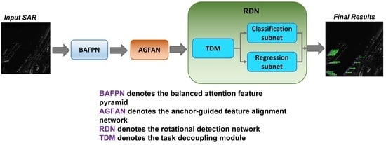
• Balanced rotated feature-aligned network (RBFA-Net) is proposed for SAR ship recognition.
• A balanced-attention FPN is used for fusing multi-scale features and reducing the negative impact of the imbalance of different scale ships.
• A rotational detection module is used for fixing the position of ships with rotated bounding boxes and classifying the categories of ships.

The rest of this paper is arranged as follows. Section 2 introduces the methodology. Experiments are described in Section 3. Results and ablation studies are shown in Section 4. Finally, a summary of this paper is put forward in Section 5.

2. Proposed Methods

RBFA-Net is designed on the basis of RetinaNet [13], which consists of FPN and detection subnets. First, we improve the detection subnets with rotated anchors where RetinaNet uses horizontal anchors. Then, we use the BAFPN instead of the FPN originally used by RetinaNet to enhance feature extraction ability. In addition, we add an anchor-guided feature alignment network after FPN to solve the misalignment between the features and rotated anchors. Finally, unlike RetinaNet directly inputting the features into the classification and regression subnets, we add TDN to solve the conflict problem before inputting the features into the classification and regression subnets.

The whole framework of RBFA-Net is divided into three parts: (1) a balanced-attention FPN (BAFPN), (2) an anchor-guided feature alignment network (AFAN) and (3) a rotational detection network (RDN). BAFPN is used for feature extraction, fusion and enhancement. AFAM is used for decreasing the dislocation between the rotated anchor boxes and feature maps. RDN is used for fixing the position of ships with rotated bounding boxes and classifying the categories of ships. The architecture of RBFA-Net is shown in Figure 3.

In this section, we will first introduce BAFPN, and then, we will explain AFAM. Finally, we will introduce RDN in detail. At the end of this section, we will introduce our loss function.

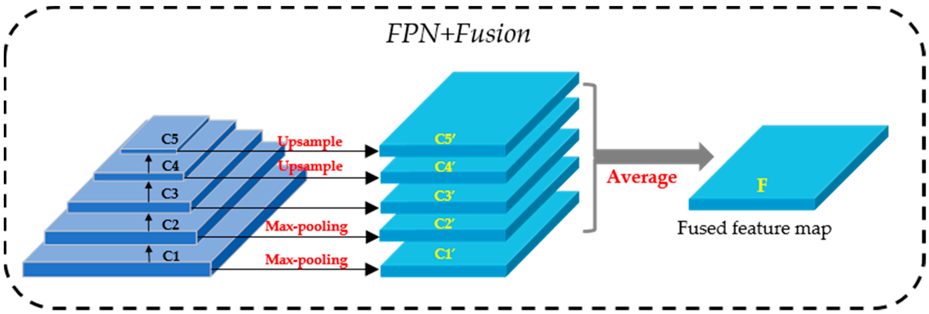
2.1. Balanced-Attention FPN

Previous works [40,41,42,43,44] tended to use the feature pyramid network (FPN) [45] as the backbone because the low-level feature maps with higher resolution are suitable for small-scale ship detection, while the high-level feature maps with more semantic information are very suitable for large-scale objects. However, using horizontal connection to integrate multi-level information makes the network pay more attention to the feature maps of adjacent layers, and the semantic information of non-adjacent layers will be diluted many times in the network. In SAR ship datasets [21,46,47], the scale span of the SAR ship target tends to be very large, which makes the ship features exhibit significant difference. In order to solve this problem, inspired by Ref. [48], we use a balanced-attention FPN (BAFPN) to balance and enhance the feature maps of different scales. As shown in Figure 3, BAFPN mainly consists of three parts: (1) feature extraction and fusion, (2) self-attention enhancement module, (3) feature pyramid recovery.

2.1.1. Feature Extraction and Fusion

Considering the feature dilution caused by multi-level horizontal connection structure in traditional FPN, we adopt another way for feature fusion. First, we use ResNet-50 to extract feature maps of different scales. As shown in Figure 4, the extracted feature maps of five levels are denoted by {$\mathit{C}\mathbf{1}$, $\mathit{C}\mathbf{2}$, $\mathit{C}\mathbf{3}$, $\mathit{C}\mathbf{4}$, $\mathit{C}\mathbf{5}$}. Since $\mathit{C}\mathbf{3}$ is in the middle of the pyramid, we recognize that $\mathit{C}\mathbf{3}$ can synthesize top semantic information and bottom spatial information better [48]. So, we resize {$\mathit{C}\mathbf{1}$, $\mathit{C}\mathbf{2}$, $\mathit{C}\mathbf{4}$, $\mathit{C}\mathbf{5}$} to the $\mathit{C}\mathbf{3}$ resolution with up-sampling and max-pooling. The rescaled feature maps are denoted by {${\mathit{C}\mathbf{1}}^{\mathbf{\prime }}$, ${\mathit{C}\mathbf{2}}^{\mathbf{\prime }}$, ${\mathit{C}\mathbf{3}}^{\mathbf{\prime }}$, ${\mathit{C}\mathbf{4}}^{\mathbf{\prime }}$, ${\mathit{C}\mathbf{5}}^{\mathbf{\prime }}$}.

Then, we fuse these rescaled feature maps by averaging, and the result is executed by

$$\mathit{F}={\displaystyle \sum }_{i=1}^5{\mathit{C}}_i^{\mathbf{\prime }}$$

(1)

where $i$ represents the $i$-th detection.

During averaging, the fused feature map obtains information from all resolutions. By using feature fusion, the impact of different ship scales on detection and classification performance can be reduced.

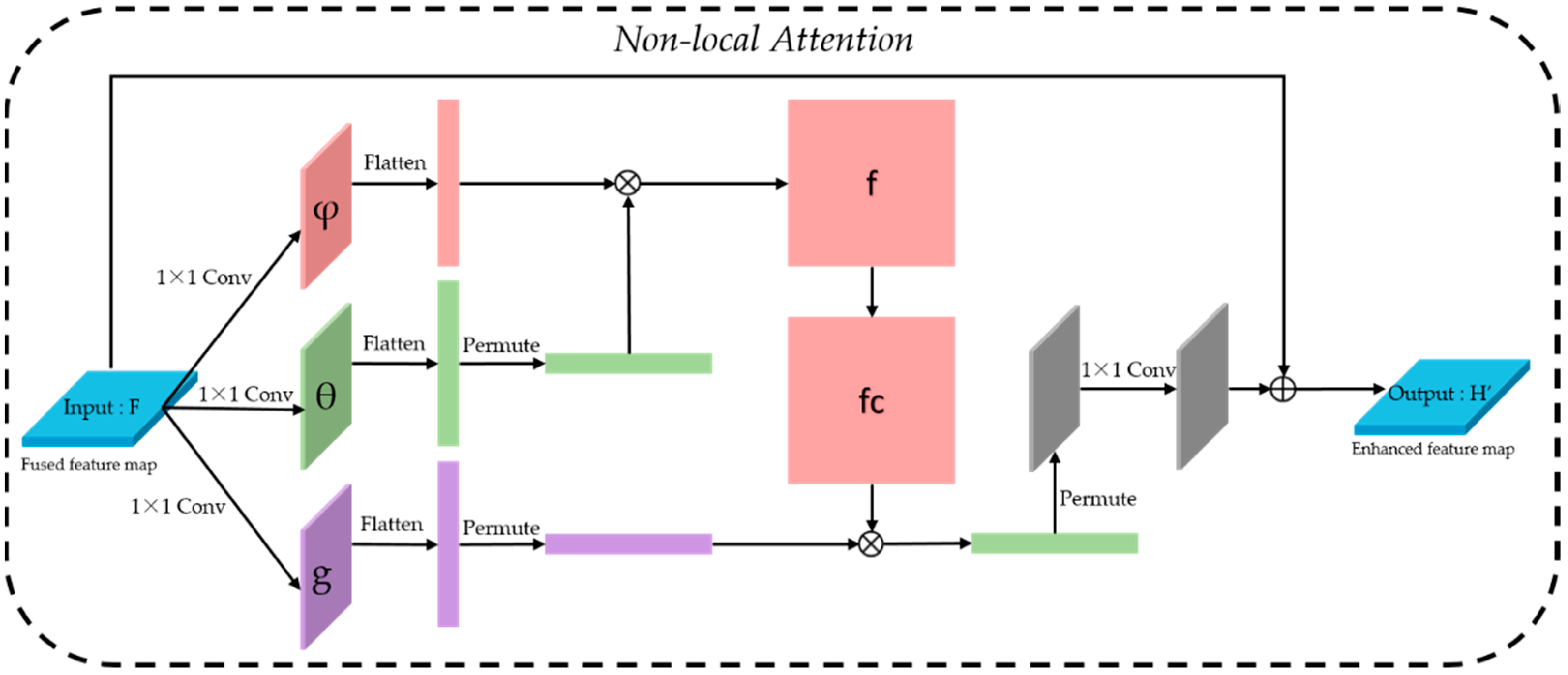
2.1.2. Attention Module

In order to enhance the global response ability of receptive field and avoid the more complex network structure caused by stacking convolution, we use the non-local [49] module to enhance the fused feature map. Through the module based on a self-attention mechanism, the network can pay more attention to the more important global information. The non-local module establishes the correlation between the global information and the local information without stacking the convolution kernels. This is equivalent to expanding the field of vision, so that the network can better integrate the global information of the image. The expression of the non-local attention formula is as follows:

$${\mathit{H}}_i=\frac{1}{C\left(\mathit{F}\right)}{\displaystyle \sum }_{\forall j}f\left({\mathit{F}}_i,{\mathit{F}}_j\right)g\left({\mathit{F}}_j\right)$$

(2)

where ${\mathit{F}}_i$ represents the $i$-th location of the input feature map.$C(·)$ represents the normalized coefficient. Function $f(·)$ is used for calculating the similarity between ${\mathit{F}}_i$ and ${\mathit{F}}_j.$ Function $g(·)$ is used for calculating the representation of the input feature map at $j$-th location. Coefficient $\frac{1}{C\left(\mathit{F}\right)}$ is used for normalization.

In order to express it concisely, the function $g(·)$ can be regarded as a linear embedding, i.e.,

$$g\left({\mathit{F}}_j\right)={\mathit{W}}_g{\mathit{F}}_j$$

(3)

where ${\mathit{W}}_g$ is the weight matrix.

In this module, we use the embedded Gaussian as the function $f(·).$ Embedded Gaussian is a simple extension of Gaussian and calculates the similarity of embedded space.

$$\begin{gathered} f\left({\mathit{F}}_i,{\mathit{F}}_j\right)=e^{\theta {\left({\mathit{F}}_i\right)}^T\phi \left({\mathit{F}}_j\right)} \\ \theta \left({\mathit{F}}_i\right)={\mathit{W}}_{\theta }{\mathit{F}}_i \\ \phi \left({\mathit{F}}_j\right)={\mathit{W}}_{\phi }{\mathit{F}}_j \end{gathered}$$

(4)

where $\theta (·)$ and $\phi (·)$ is the weight matrix. ${\mathit{W}}_{\theta }$ and ${\mathit{W}}_{\theta }$ are the weight matrices.

In addition, the normalized coefficient $C(·)$ is

$$C\left(\mathit{F}\right)={\displaystyle \sum }_{\forall j}f\left({\mathit{F}}_i,{\mathit{F}}_j\right)$$

(5)

Therefore, through the above formula, we can deduce that the output expression is

$${\mathit{H}}_i=({\displaystyle \sum }_{\forall j}{e}^{\theta {({\mathit{F}}_i)}^T\phi ({\mathit{F}}_j)}\times {\mathit{W}}_g{\mathit{F}}_j)/{\displaystyle \sum }_{\forall j}f({\mathit{F}}_i,{\mathit{F}}_j)$$

(6)

Figure 5 shows the architecture of the non-local module. We put the input feature maps $\mathit{F}$ into three $1\times 1$ convolutional layers at the same time to calculate $\mathsf{\phi }$, $\mathsf{\theta }$ and $\mathsf{g}$. Then, we flatten the H and W dimensions of $\mathsf{\phi }$ and $\mathsf{\theta }$. With the flattened layers, we can calculate the similarity $f$ by matrix multiplication. Finally, the similarity $f$ is normalized by a soft-max function, and the result is multiplied by the flattened feature maps $\mathit{g}$. The output is also processed by a $1\times 1$ convolution layer to make it match the size of the input feature map. Apart from that, a skip connect is added into the architecture. So, the final output refined feature map ${\mathit{H}}^{\prime }$ is

$${\mathit{H}}^{\mathbf{\prime }}={\mathit{W}}_H\mathit{H}+\mathit{F}$$

(7)

where ${\mathit{W}}_H$ is the weight matrix.

For example, for the input feature map $\mathit{F}$, the following operations are performed in the non-local module:

• Use $1\times 1$ convolution for down-sampling to obtain three variants: $\mathsf{\phi }$, $\mathsf{\theta }$ and $\mathit{g}$.
• $\mathsf{\phi }$ and $\mathsf{\theta }$ perform channel merging and transposing, respectively, and then perform matrix multiplication to gain similarity $f$.
• The similarity $f$ is normalized by a soft-max function, and then multiply $f$ with the channel-merged $\mathit{g}$.
• The obtained results first restore the original size and then restore the number of channels through $1\times 1$ convolution.
• Finally, add it to the original input $\mathit{F}$ to form a complete residual non-local module.

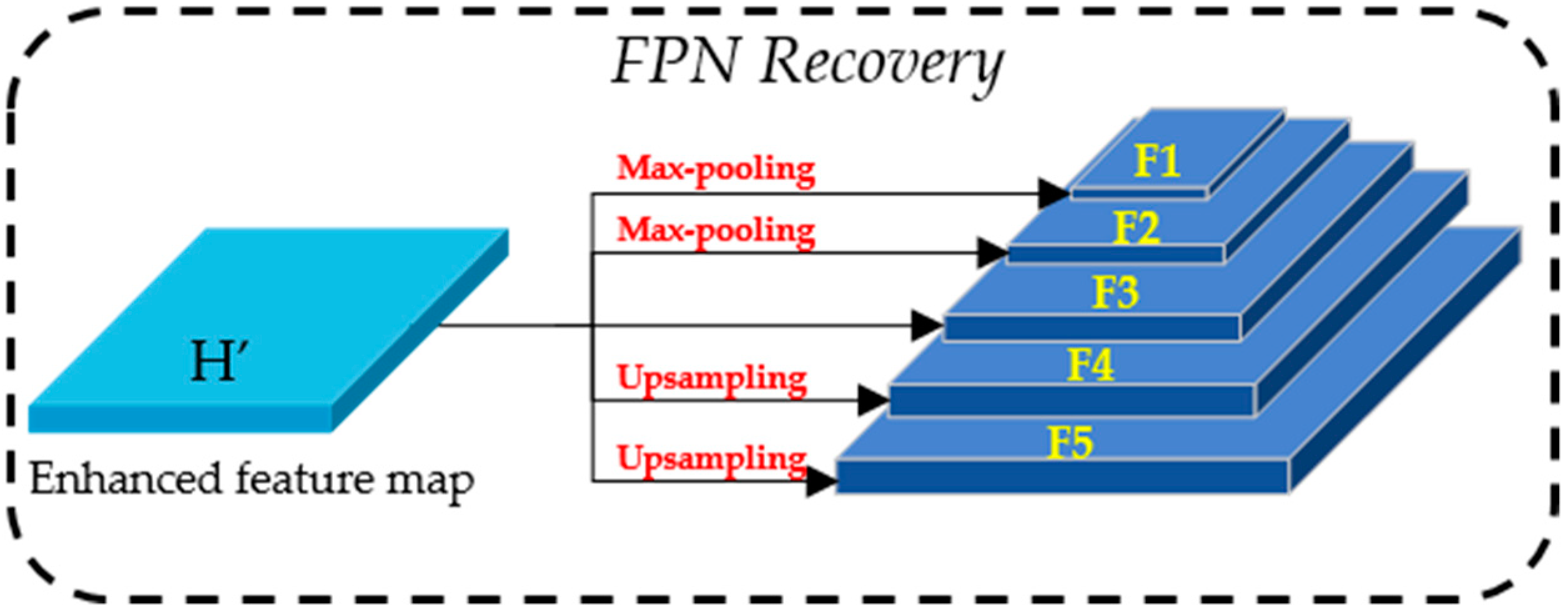
2.1.3. Feature Pyramid Recovery

As shown in Figure 6, the fused feature maps are restored to a feature pyramid through up-sampling and max-pooling. This part can be regarded as the reverse operation of feature fusion. As shown in Figure 6, the enhanced feature maps ${\mathit{H}}^{\prime }$ from the non-local module are restored to a feature pyramid consisting of five levels {$\mathit{F}\mathbf{1}$, $\mathit{F}\mathbf{2}$, $\mathit{F}\mathbf{3}$, $\mathit{F}\mathbf{4}$, $\mathit{F}\mathbf{5}$}. Among them, {$\mathit{F}\mathbf{1}$, $\mathit{F}\mathbf{2}$} are obtained from ${\mathit{H}}^{\prime }$ through max-pooling. {$\mathit{F}\mathbf{4}$, $\mathit{F}\mathbf{5}$} are obtained from ${\mathit{H}}^{\prime }$ through up-sampling. Feature maps ${\mathit{H}}^{\prime }$ are retained as $\mathit{F}\mathbf{3}$ in the recovered feature pyramid. In the recovered feature pyramid, each level contains more multi-scale features and balanced information from all resolutions. To conclude, the BAFPN enables RBFA-Net to better focus on multi-scale ship features while integrating global features.

2.2. Anchor-Guided Feature Alignment Network

In networks using horizontal anchors, the convolution features are aligned with anchors, so the convolution features can reflect the anchor representations [30]. However, in the network using rotating anchor, solving the misalignment between rotated anchors and convolution features is an important problem. To solve this problem, we introduce an anchor-guided feature alignment network. With the guidance of rotated anchors, the feature map will be adjusted to align with rotated anchors in the next rotational detection network. In this section, we will first introduce the basic information about the rotated bounding box and then introduce the anchor-guided feature alignment network.

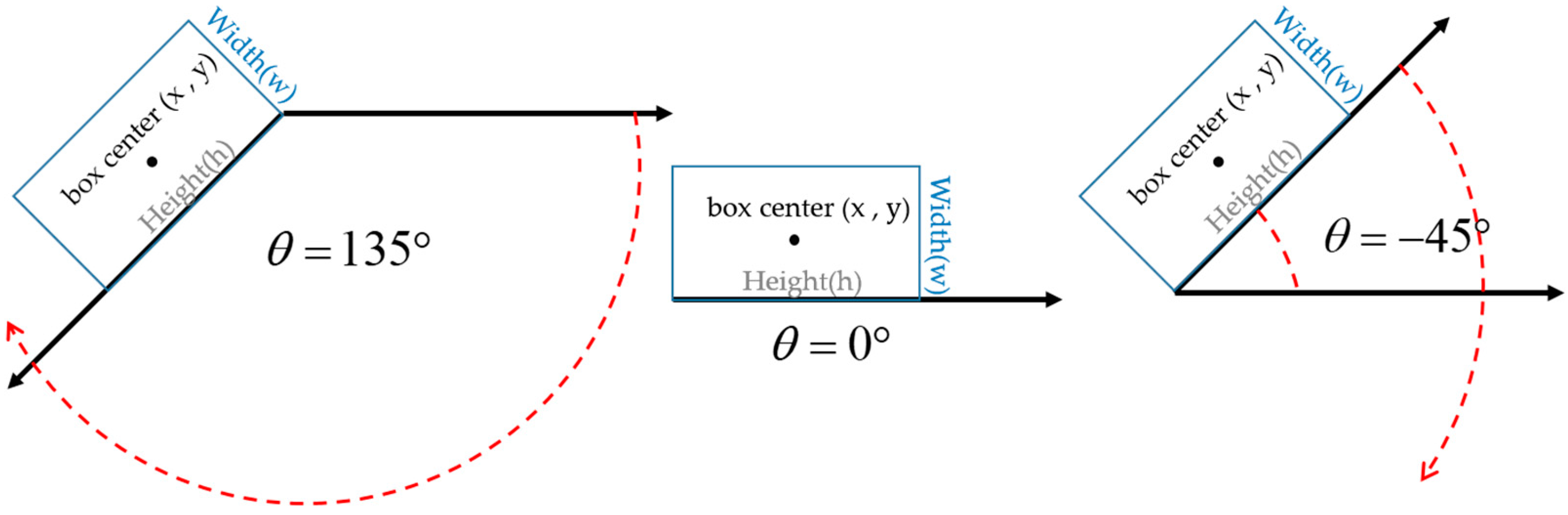
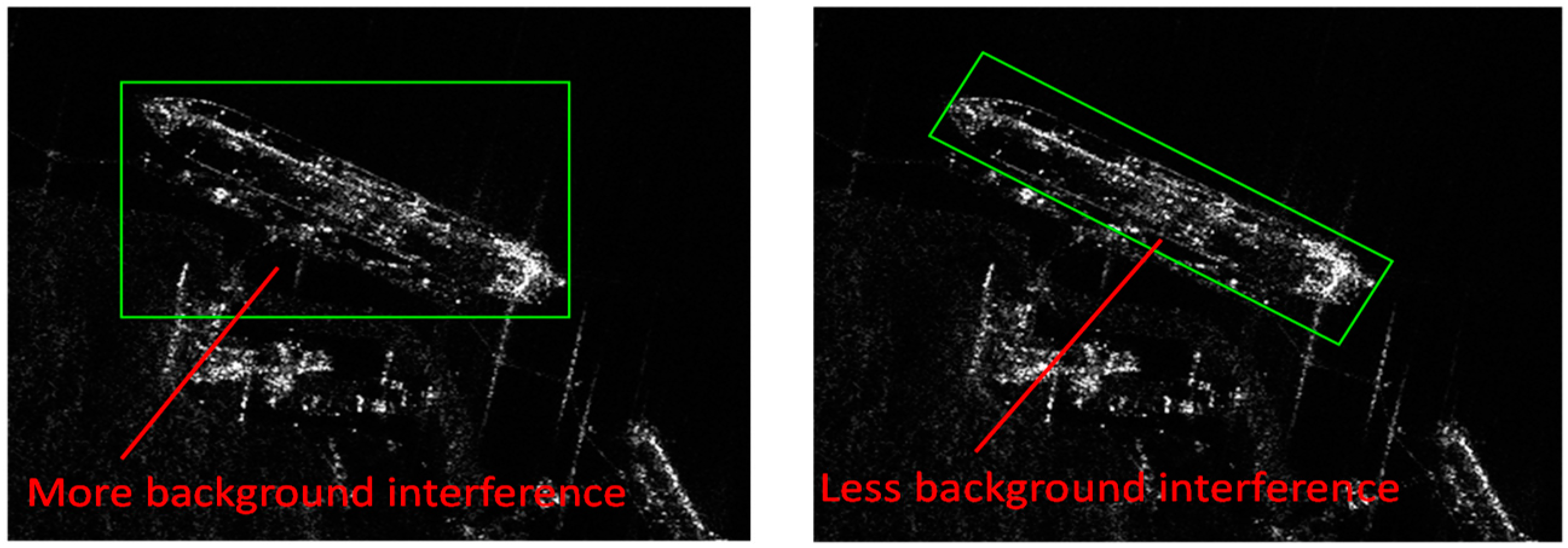
2.2.1. Introduction to Rotated Bounding Box

In this paper, we use the geometric definition of the rotated bounding box used by MMRotate [50]. The rotated bounding box can be represented by five parameters $\left(x,y,w,h,\theta \right)$. The two tuples $\left(x,y\right)$ represtent the location of the center point of the rotated bounding box. The two tuples $\left(w,h\right)$ represent the length and width of the rotated bounding box. $\theta$ is the rotation angle of the rotated bounding box, and its value range is $\left[-45°,135°\right)$. Figure 7 shows more details about the geometric definition of the rotated bounding box.

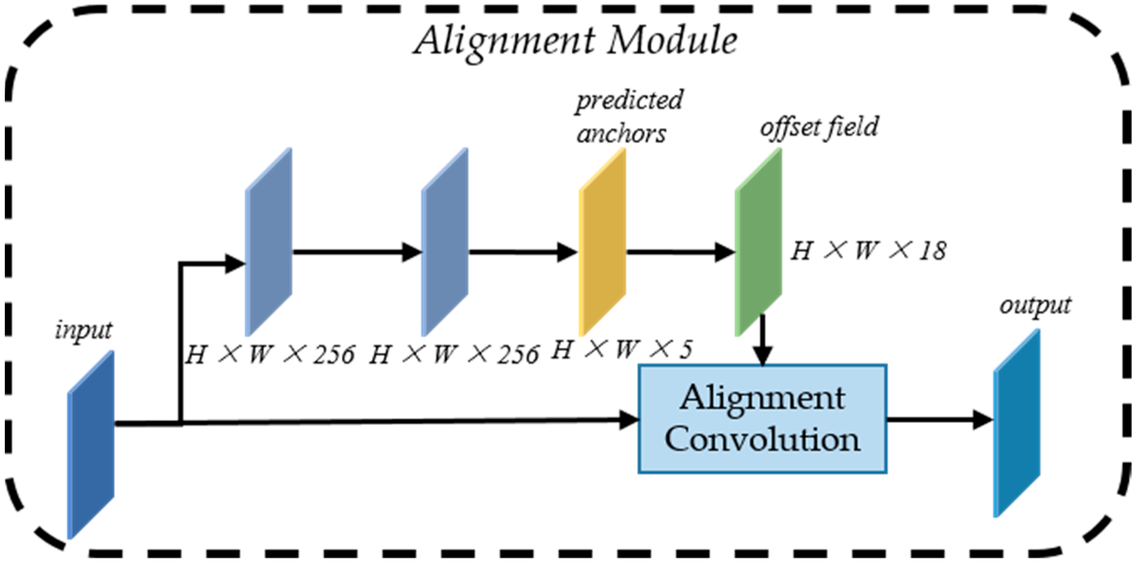
2.2.2. Anchor-Guided Feature Alignment Network

Generally, many existing networks with a rotated bounding box use heuristically defined anchors with different scales and aspect ratios. As a result, these networks tend to suffer from misalignment between the rotated anchor boxes and axis-aligned convolution features. Previous works [30,51] have proved that this misalignment will lead to the decline of detection accuracy. In order to solve this problem, we introduce the alignment convolution layer to establish the anchor-guided feature alignment network (AFAN) to extract the adaptive features according to the predicted shape of the refined anchor.

The core idea of AFAN is that we use the alignment convolution layer to reset the sampling locations according to the roughly generated rotated bounding box. As shown in Figure 8, the extracted feature maps are sent into a rough regression subnet consisting of two convolution layers. The subnet roughly generates rotated bounding boxes in this part. Then, through these roughly generated bounding boxes, we can calculate their offset from the bounding boxes. Finally, these offsets and the original feature maps are put into the alignment convolution layer to reset the sampling locations.

For the feature maps extracted through BAFPN, firstly, they will be input into a regression network to preliminarily locate the anchors and adjust their directions. From this, we obtain the feature maps of $H\times W\times 5$. For each 5-dimensional anchor box, we sample 9 points to obtain the 18-dimension offset field $O$. The calculation formula of the offset field $O$ is as follows:

$$L_{p_0}^{p_k}=\frac{1}{S}(\left(x,y\right)+\frac{1}{k}\left(w,h\right)p_k)R^T\left(\theta \right)$$

(8)

$$O={\left\{L_{p_0}^{p_k}-p_o-p_k\right\}}_{p_k\in R}$$

(9)

where $L_{p_0}^{p_k}$ represents the sampling location. $S$ represents the stride of the feature maps. $k$ represents the kernel size. $p_0$ represents each location on the feature map ${\mathit{X}}_A$. $p_k$ represents the $p_k$-th location in ${\mathit{X}}_A$. $R\left(\theta \right)={\left(cos\theta ,-sin\theta ;sin\theta ,cos\theta \right)}^T$ is the rotation matrix. $\mathit{O}$ represents the offset field.

Finally, the offset field and feature maps extracted with BAFPN are input into the alignment convolution layer. By alignment convolution, we align the feature maps with the rotated bounding boxes. These aligned feature maps will be input into RDN for ship target detection and classification.

The alignment convolution is established by adding the offset field $o$ to the ordinary convolution. The alignment convolution can be defined as follows:

$${\mathit{X}}_A\left(p_o\right)={\displaystyle \sum }_{p_k\in R,o\in O}\mathit{w}\left(p_k\right)\mathit{X}\left(p_o+p_k+o\right)$$

(10)

o represents the offset in the offset field $\mathit{O}$.

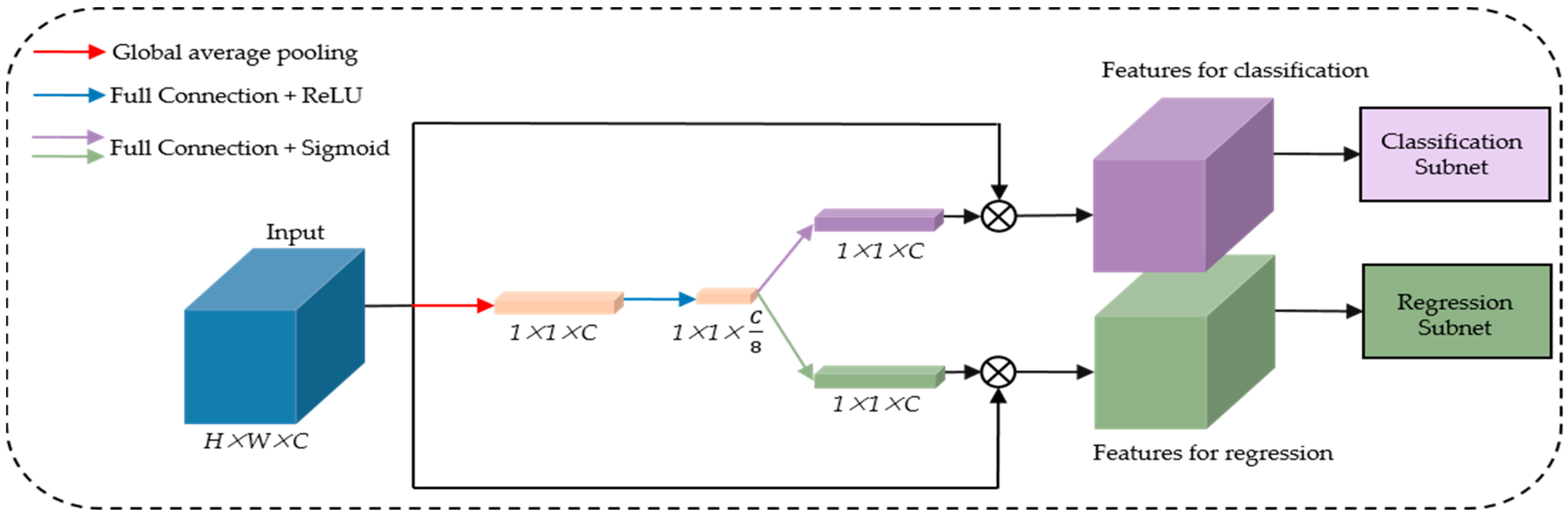
2.3. Rotational Detection Network

In this section, we propose a rotational detection network (RDN) to realize ship detection and classification. RDN is designed on the basis of RetinaNet [13], where the feature maps are sent to the regression subnet and classification subnet, respectively. However, the features used for classification should remain invariant, while for the regression task, the features should represent the changes of the target position, size and rotation angle. The opposite requirements bring negative impact on detection accuracy. In order to solve this conflict, we propose a task decoupling module. Recent studies [52] have shown that decoupling the classification task and regression task in the spatial dimension of the feature maps can relieve this conflict. Therefore, we add a task decoupling module consisting of two squeeze-and-excitation (SE) modules [53]. Figure 9 shows the architecture of the rotational detection network.

As shown in Figure 9, a global average pooling layer, a full connection layer and a ReLU activation function form the encoder of the task decoupling module. For the feature maps from AFAN, their dimension is $H\times W\times C$. Firstly, these feature maps are put into the global average pooling layer to extract the global feature information. Then, we send the output feature maps of the global pooling layer to a full connection layer and a ReLU activation function [54]. According to the design of SENet, the size of the output feature map is compressed to $1\times 1\times C/8$. Then, the output of the encoder will be input into two decoders composed of a full connection layer and a sigmoid activation function, respectively, and the size will be restored to $1\times 1\times C$ in this process. Finally, the feature maps are multiplied by the corresponding elements in the decoder output vector to adjust the feature maps to adapt to different learning tasks. The output feature maps are sent to the classification subnet and regression subnet, respectively.

2.4. Loss Function

The loss function of RBFA-Net is composed of two parts: the loss of AFAN and the loss of RDN. Each part consists of classification loss and regression loss. The loss of AFAN is similar to that of RDN. Both of them are obtained by adding regression loss and classification loss. The formulae are as follows:

$$\begin{gathered} L=\frac{1}{N_A}{L}_{AFAN}+\frac{\lambda }{N_D}{L}_{RDN} \\ {L}_{AFAN}={\displaystyle \sum }_{i=1}^N{L}_{cls}\left(p_i^A,p_i^{*}\right)+{\displaystyle \sum }_{i=1}^N{p}_i^{*}{L}_{reg}\left({\mathit{t}}_i,{\mathit{t}}_i^{*}\right) \\ {L}_{RDN}={\displaystyle \sum }_{i=1}^N{L}_{cls}\left(p_i,p_i^{*}\right)+{\displaystyle \sum }_{i=1}^N{p}_i^{*}{L}_{reg}\left({\mathit{t}}_i^D,{\mathit{t}}_i^{*}\right) \end{gathered}$$

(11)

where $p_i$ represents the predictive class probability, $p_i^{*}$ represents the ground-truth category. $p_i^{*}=1$ when sample $I$ is a positive one, else $p_i^{*}=0$. $p_i^A$ indicates that the prediction probability is obtained by AFAN. $\lambda$ is a hyper-parameter to balance the loss of the alignment network and that of the detection network. ${\mathit{t}}_i^{*}$ represents the offset between the $i$-th sample and ground truth. ${\mathit{t}}_i$ represents the offset between the $i$-th prediction and ground truth. ${\mathit{t}}_i^D$ indicates that the offset is obtained by RDN. We use focal loss [13] and balanced L1 loss [48] as the classification loss $L_{cls}$ and regression loss $L_{reg}$.

The main purpose of the regression subnet is predicting the location, size and angle of the rotated bounding boxes. According to the definition of the rotated bounding box, the regression offset $t_i^{*}$ and $t_i$ can be denoted by

$$\begin{gathered} t_x^{*}=\frac{G_x-A_x}{A_w}, t_y^{*}=\frac{G_y-A_y}{A_h} \\ {t}_w^{*}=log\frac{G_w}{A_w}, t_h^{*}=log\frac{G_h}{A_h} \\ {t}_{\theta }^{*}=\tan \left(G_{\theta }-A_{\theta }\right) \\ {t}_x=\frac{B_x-A_x}{A_w}, t_y=\frac{B_y-A_y}{A_h} \\ {t}_w=log\frac{B_w}{A_w}, t_h=log\frac{B_h}{A_h} \\ {t}_{\theta }=\tan \left(B_{\theta }-A_{\theta }\right) \end{gathered}$$

(12)

where $G_i$, $A_i$ and $B_i$ represent the five-tuple coordinate $i\in \left(x,y,w,h,\theta \right)$ of ground truth, anchor box and predicted bounding box. $t_i^{*}$ represents the regression offset between the ground truth and anchor box. $t_i$ represents the regression offset between the predicted bounding box and anchor box.

Like Refs [13,55,56], we use focal loss as the classification loss $L_{cls}$. However, previous work proved that the imbalance of classification loss and regression loss has negative impact on the detection accuracy. Directly adjusting the weight to increase the regression loss will make the network more sensitive to outliers, which is unfavorable for SAR images with much speckle noise. So, we use balanced L1 loss as the regression loss $L_{reg}$ instead of the widely used smooth L1 loss.

Researchers usually balance the regression loss and classification loss by adjusting the loss weight. However, directly increasing the weight of regression loss will make the model more sensitive to the noise in the image. Moreover, SAR images are often disturbed by much background noise and speckle noise, which seriously affects the detection accuracy. Therefore, to solve this problem, we use balanced L1 loss instead of the commonly used smooth L1 loss as the regression loss. The formula of balanced L1 loss is as follows:

$$L_b\left(x\right)=\{\begin{array}{c}\frac{a}{b}\left(b\left|x\right|+1\right)ln\left(b\left|x\right|+1\right)-a\left|x\right|, if \left|x\right|<1\\ \gamma \left|x\right|+C , otherwise\end{array}$$

(13)

where $a,b$ and $\gamma$ are hyper-parameters and meet $aln\left(b+1\right)=\gamma$. According to the configuration in Ref. [48], we set $a=0.5$, $\gamma =1.5$. $x$ is the difference between the predicted value and the ground truth.

As Ref. [48] points out, compared with smooth L1 loss, balanced L1 loss can increase more gradient for accurate samples, reducing the contribution of outliers to loss. For example, compared with the contribution of outliers, the contribution of inliers to loss is only 30%, which makes the network very sensitive to outliers. Using balanced l1loss can improve the contribution of normal values to loss and reduce the sensitivity of the network to outliers. Therefore, using balanced L1 loss is helpful for ship detection, especially for ship detection in inshore scenes.

3. Experiments

Our experiments are run on a personal computer with i9-9900K CPU and RTX2080Ti GPU based on Pytorch. Our experiments are under the MMDetection toolbox [57] to ensure comparison fairness.

3.1. Experimental Datasets

One of the main reasons for the lack of research on SAR ship recognition in the past has been insufficient data. Now, thanks to the SAR rotation ship detection dataset (SRSDD) released by Lei et al. [22] in 2021, the research on SAR ship detection and classification can be further developed. The images in SRSDD all come from China’s GF-3 satellite, which photographed more than 30 ports from five locations. The size of each slice is $1024\times 1024$.

Table 1. The basic parameters of SRSDD.

Parameter	Value
Number of images	666
Waveband	C
Image Size	$1024 \times$1024
Image Mode	Spotlight Mode
Polarization	HH, VV
Resolution(m)	1
Ship Classes	6
Position	Nanjing, Hongkong, Zhoushan, Macao, Yokohama

shows more details about SRSDD.

The ships in SRSDD are marked by the rotated bounding box and are divided into six categories, including ore–oil ships, bulk cargo ships, fishing boats, law enforcement ships, dredger ships and container ships. The rotated bounding box and the category of each ship target are given by experts after checking the corresponding SAR image and corresponding optical image. This ensures their authenticity and accuracy.

Table 2. The number of each ship category in SRSDD.

Category	Train Number	Test Number	Total Number
Ore–oil ships	132	34	166
Bulk cargo ships	1603	450	2053
Fishing boats	206	82	288
Law enforcement	20	5	25
Dredger ships	217	46	263
Container ships	67	22	89
Total	2245	639	2884

shows the number of each category. It can be seen from the table that the number of bulk cargo accounts for most of the total, while the number of law enforcement is almost one tenth of that of bulk cargo.

In addition, considering the problem that the number of offshore scenes is larger than that of inshore scenes in the existing SAR dataset, such as SSDD [21,46] and Gaofen-SSDD [47], SRSDD focuses on taking nearshore scenes during sampling. In SRSDD, inshore scenes account for 63.1%, and offshore scenes account for 36.9%. In order to ensure fairness of the experimental results, our experiment is completely consistent with Ref. [22], that is, 532 pictures are used for training, and 134 pictures are used for testing.

3.2. Experimental Details

We refer to the work of Pang et al. [48] and use Resnet-50 [58] pretrained on Image-net as the backbone of RBFAN. A large number of images in Image-net can better train Resnet-50 to extract underlying features. Limited by GPU, we set the batch size to 4. Similar to Ref. [59], we use stochastic gradient descent (SGD) [60] as the optimizer, with a 0.005 learning rate, 0.9 momentum and 0.0001 weight. In addition, the learning rate is reduced from 130 epochs to 140 epochs, and each epoch is reduced by 10 times to ensure sufficient loss reduction. In addition, the intersection of union (IOU) threshold in the experiment is set to 0.5. According to the configuration in Ref. [48], we set $a=0.5$, $\gamma =1.5$. The hyper-parameter $\lambda$ in loss function is set to 1. The hyper-parameter $C$ in balanced L1 loss is set to 0.5.

According to Refs [13,30,48], we set the following parameters. In BAFPN, the resolution of each layer is $\left[512\times 512, 256\times 256, 128\times 128, 64\times 64, 32\times 32\right]$. The size of the fused feature map is $128\times 128\times 256$. The resolution of the restored feature pyramid is $\left[512\times 512, 256\times 256, 128\times 128, 64\times 64, 32\times 32\right]$. In AFAN, the convolution kernel size is $3\times 3$. In RDN, the size of the used convolution kernels is $3\times 3$ for all. The number of convolution layers stacked in the classification subnet and the regression subnet is 2.

3.3. Training Process

RBFA-Net is a single-stage network, so we refer to the training method of single-stage network in MMDetection [57] during training.

The specific training process is as follows:

• Obtain the SAR image dataset preprocessed by SRSDD publisher.
• Input the SAR image data into RBFA-Net for forward propagation to obtain the regression score and classification score.
• Input the regression score and classification score and the ground truth into the loss function to obtain loss value.
• Determine the gradient vector by back propagation.
• Adjust each weight to make the loss value tend to zero or converge. We use the stochastic gradient descent (SGD) method for adjustment.
• Repeat the above process until the set number of training times (training epoch) or loss value does not decrease.

3.4. Evaluation Indices

In this paper, we use mean average precision (mAP) as the evaluation index. The larger the mAP, the higher the network detection accuracy. To calculate mAP, we need to calculate recall and precision first. The recall and precision can be calculated as

$$Recall=\frac{TP}{TP+FN}$$

(14)

$$Precision=\frac{TP}{TP+FP}$$

(15)

where TP represents the number of true positives, FN represents the number of false negatives, FP represents the number of false positives. Then, we can obtain the precision–recall curve and calculate mAP.

$$AP={{\displaystyle \int }}_0^{1}P\left(R\right)dR$$

(16)

$$mAP=\frac{1}{k}{\displaystyle \sum }_{i=1}^{k}A{P}_i$$

(17)

where $R$ represents recall, and $P$ represents precision. $P\left(R\right)$ represents the precision–recall curve.

4. Results

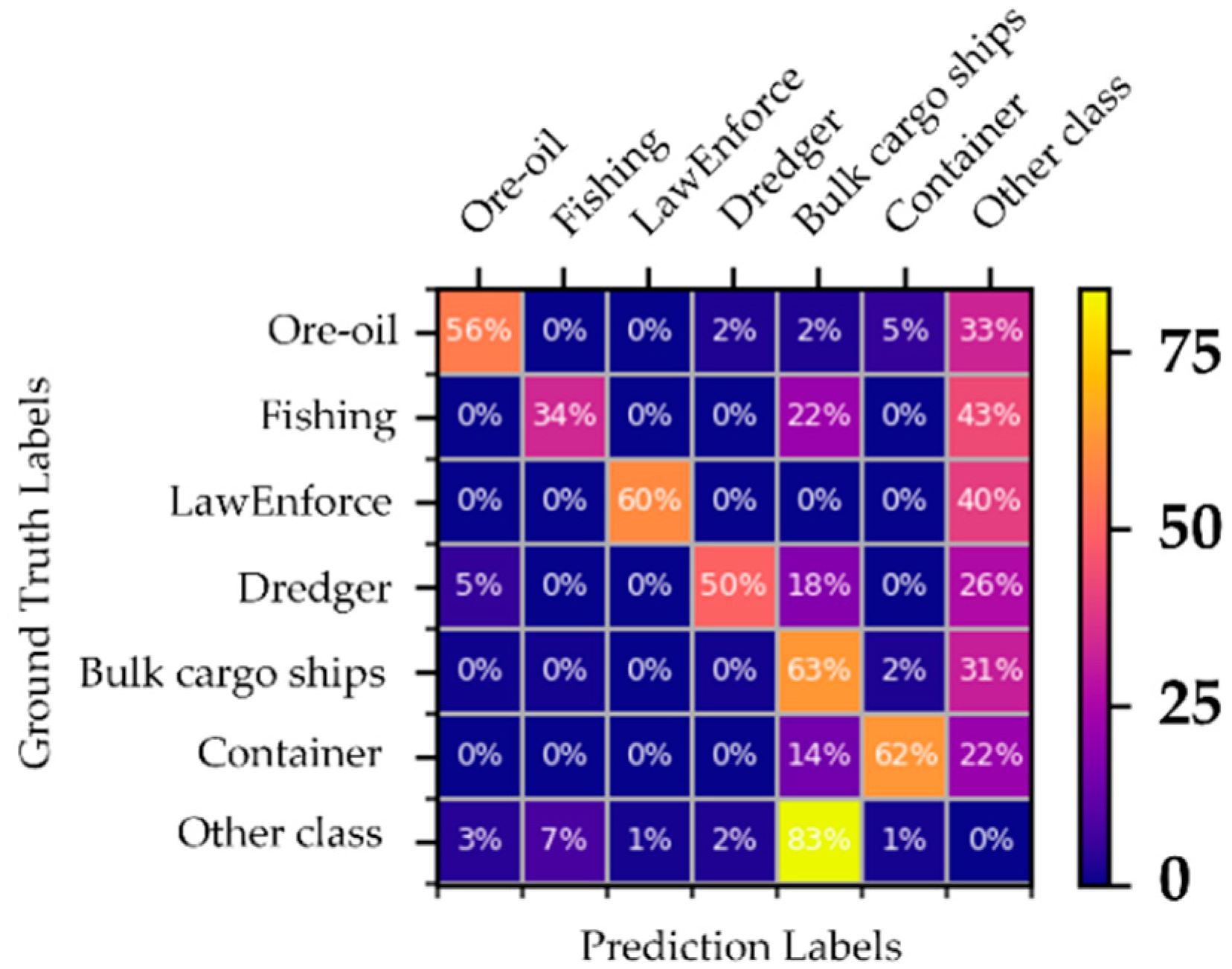
4.1. Qualitative and Quantitative Analyses of Results

Table 3. Quantitative evaluation comparison with the eight state-of-the-art detectors. Labels C1–C6 correspond to ore–oil ships, fishing boats, law enforcement ships, dredger ships, bulk cargo ships and container ships.

Models	C1	C2	C3	C4	C5	C6	mAP	Model Size
FR-O [16]	55.62	30.86	27.27	77.78	46.71	85.33	53.93	315 MB
R-RetinaNet [13]	30.37	11.47	2.07	67.71	35.79	48.94	32.73	277 MB
ROI [31]	61.43	32.89	27.27	79.41	48.89	76.41	54.38	421 MB
R3Det [55]	44.61	18.32	1.09	54.27	42.98	73.48	39.12	468 MB
BBAVectors [61]	54.33	21.03	1.09	82.21	34.84	78.51	45.33	829 MB
R-FCOS [40]	54.88	25.12	5.45	83.00	47.36	81.11	49.49	244 MB
Glid Vertex [63]	43.41	34.63	27.27	71.25	52.80	79.63	51.50	315 MB
O-RCNN [62]	63.55	35.35	27.27	77.50	57.56	76.14	56.23	315 MB
RBFA-Net (Ours)	59.39	41.51	73.48	77.17	57.36	71.62	63.42	302 MB

The best detector is in bold and the second best is underlined.

shows the comparison of the detection results with the other eight rotated detectors on SRSDD. In Table 3, labels C1–C6 correspond to ore–oil ships, fishing boats, law enforcement ships, dredger ships, bulk cargo ships and container ships. The detection results of the other methods are from Ref. [22]. It can be seen from the results that the performance of our network is better than the eight state-of-the-art methods. In addition, our RBFA-Net achieves the highest mAP with a small model size, which proves the excellent performance of our RBFA-Net. Our RBFA-Net is only half the size of BBAVectors [61]. Moreover, the size of RBFA-Net is smaller than the second-best O-RCNN [62].

For each category, except for fishing boat and dredger, our model obtains optimal or suboptimal results. For fishing boat and dredger, our detection accuracy is also above the average level. For the largest number of categories (bulk cargo) and the lowest number of categories (law enforcement) in SRSDD, our detection accuracy reaches the best, which proves that our network can not only focus on small samples but also ensure the accuracy of large sample targets. It is worth noting that the detection accuracy of our network in law enforcement category is much higher than that of other models. Because law enforcement often appears in a fixed position, it is more sensitive to spatial information. With BAFPN, our network integrates global information, so it is helpful for the detection of such spatial sensitive targets.

We also draw the confusion matrix showing the classification results of our network in more detail. The confusion matrix evaluates the classification accuracy of the network. As shown in Figure 10, the abscissa is the prediction category, and the ordinate is the real category. In the confusion matrix, the diagonal is the correct classification probability, and the others are the wrong classification probability. The confusion matrix is composed of ore–oil ships, fishing boats, law enforcement ships, dredger ships, bulk cargo ships, container ships and other class. Among them, the other class includes ships not in the dataset and other sea targets, such as oil platforms.

Limited by space, Figure 11 shows the qualitative comparison of second-best method O-RCNN [62] and our RBFA-Net in detail. In order to observe the detection results of densely arranged ships near the shore, we compare the sliced and enlarged SAR images.

From the experimental results, we can draw the following conclusions:

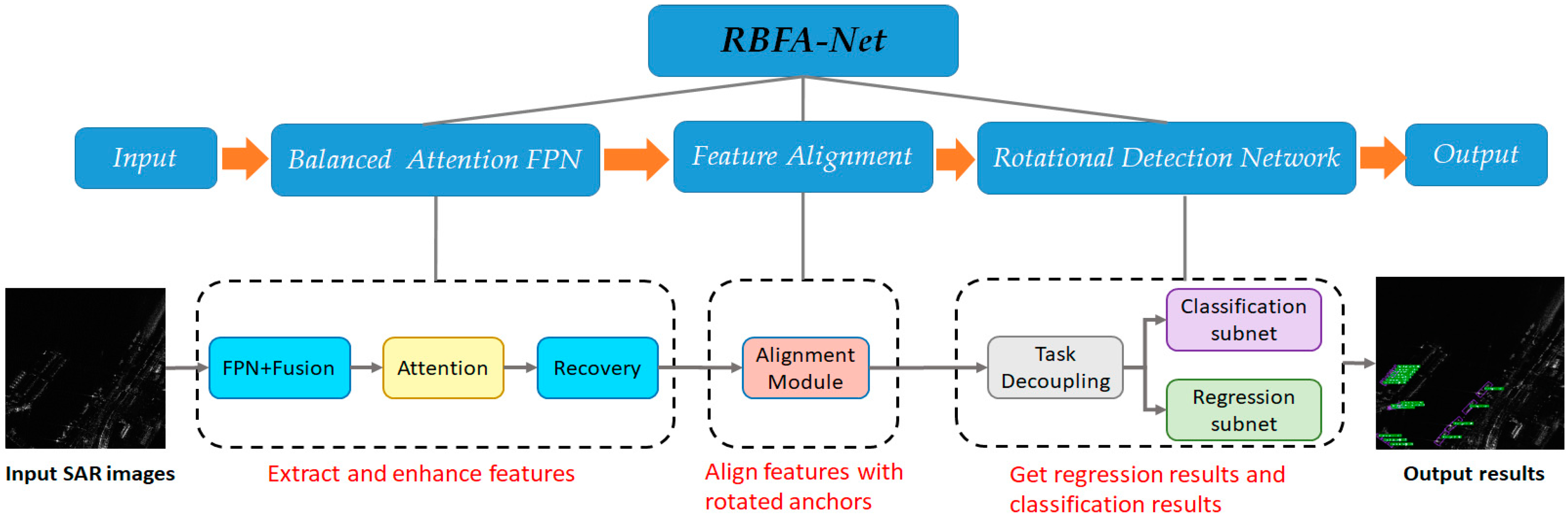
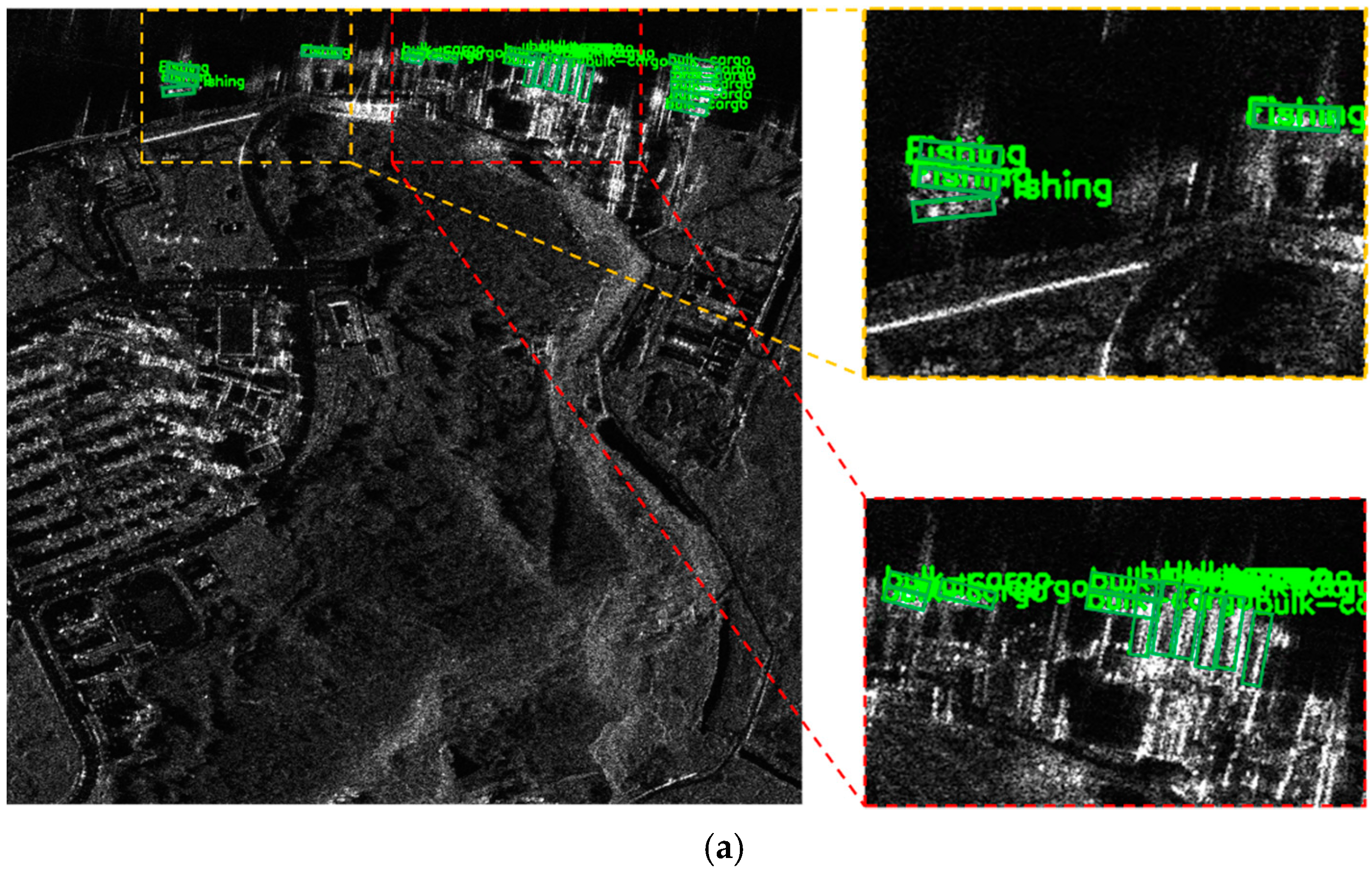
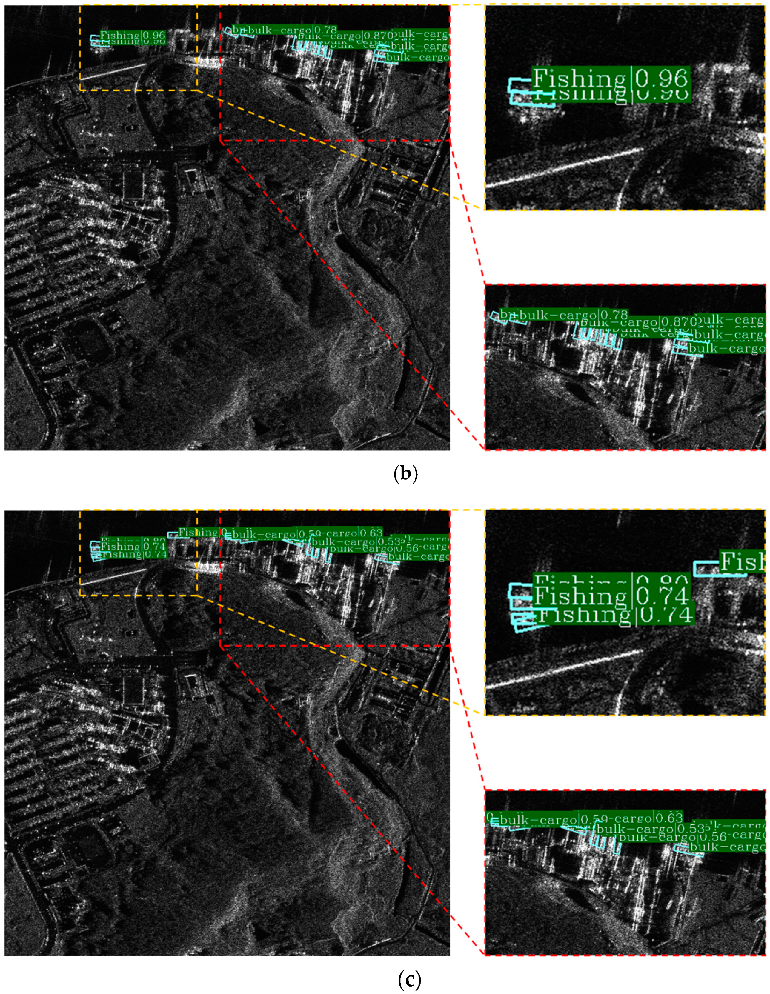
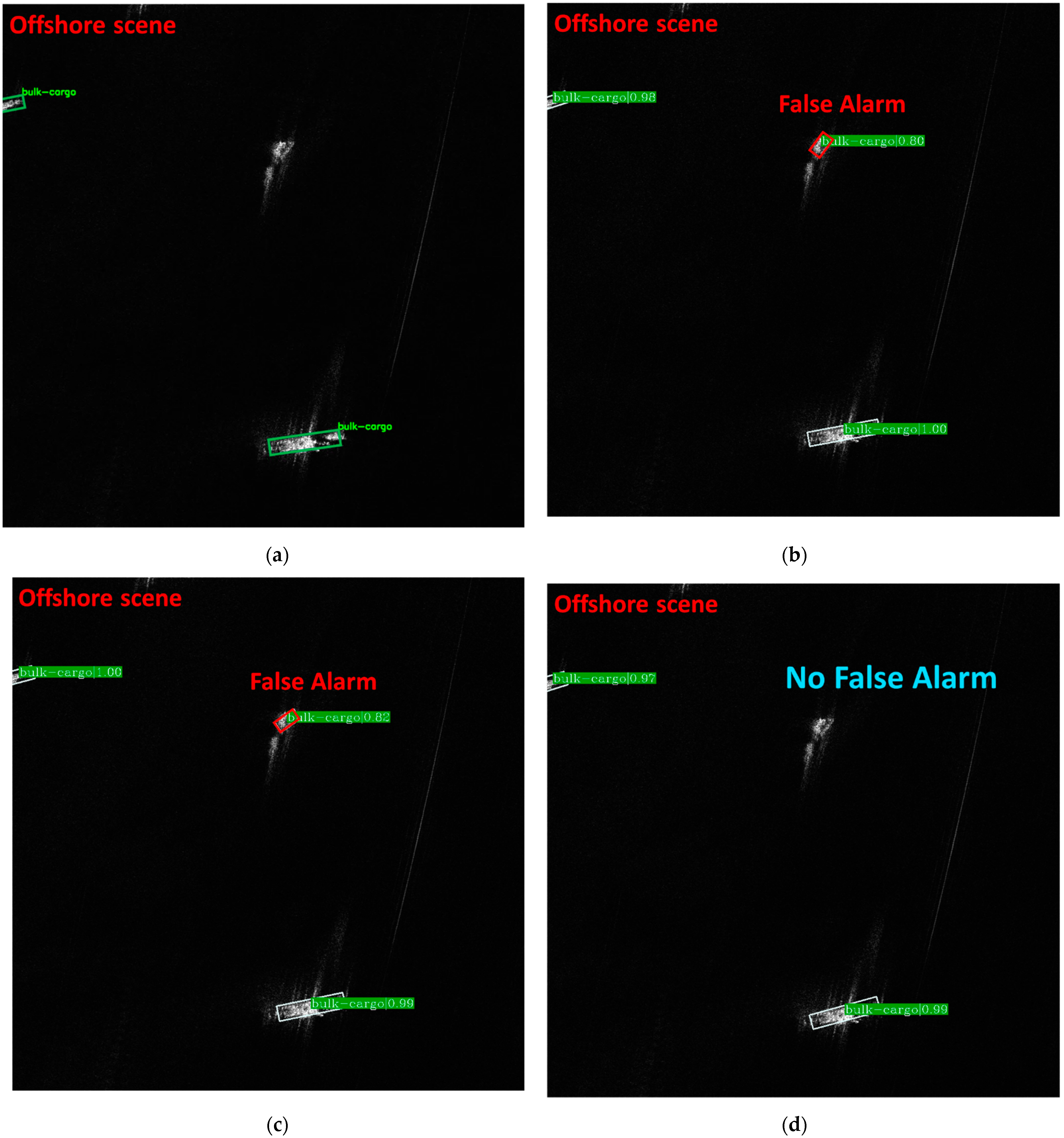
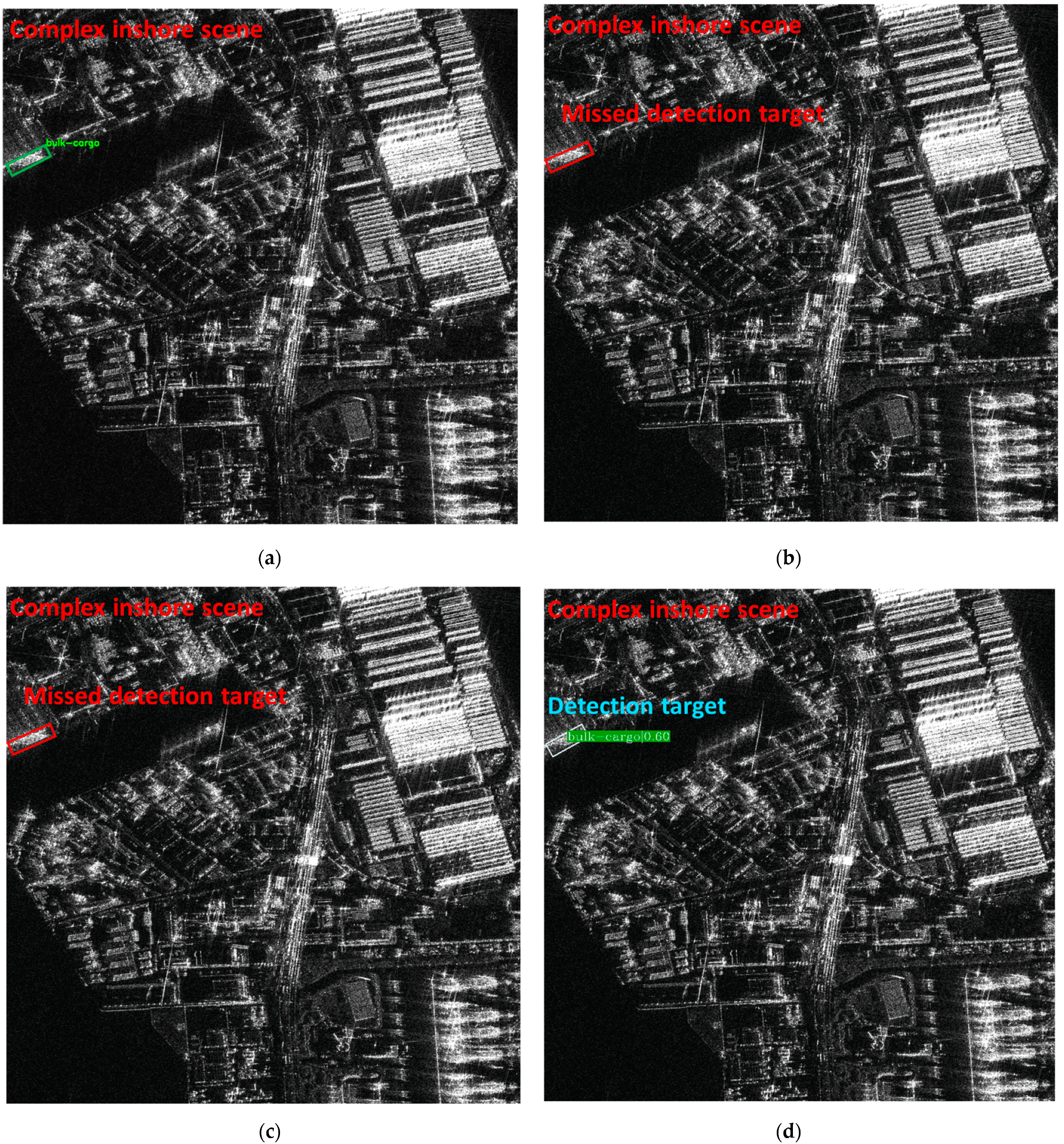
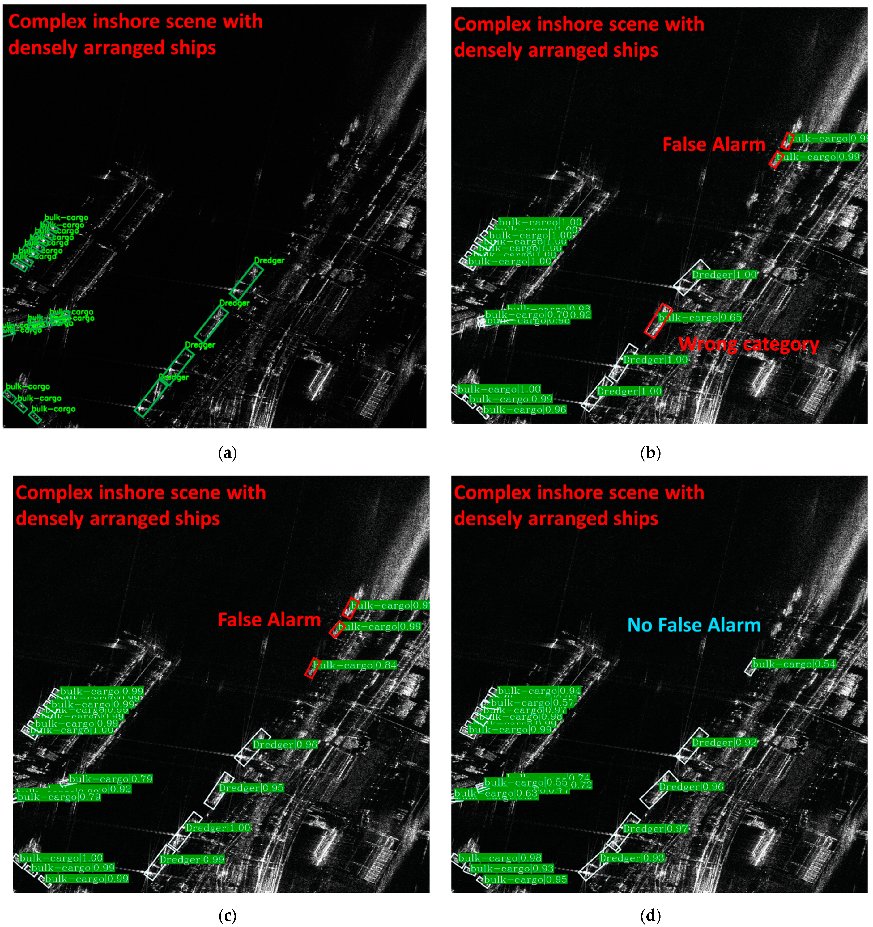
• RBFA-Net net can avoid some missing inspection of some densely arranged inshore small ships. As shown in Figure 11, RBFA-Net detects more fishing boats and bulk cargo than O-RCNN. This is because RBFA-Net uses AGFAN to align the feature map with the rotating anchor boxes, which reduces the negative impact of densely arranged ships and background interference.
• For inshore ship detection, RBFA-Net has better detection accuracy, as shown in Figure 11. In the same SAR image, RBFA-Net can detect and correctly classify the inshore ships and the complex coastal background. This is because RBFA-Net uses FAFPN to fuse and enhance multi-scale features, which enhances the ability of focusing on global information of SAR images.
• For the problem of difficult target ship detection, RBFA-Net has a higher detection effect, as shown in Figure 11. RBFA-Net can successfully classify the fishing boat, which has similar features with bulk cargo ships. This is because RBFA-Net uses the task decoupling module to adaptively enhance the feature map, making it better in the classification network.
• Nevertheless, there are still some problems in our network. For example, there is still the problem of missing inspection when there are too many nearshore ships. For some ships whose characteristics are not obvious, there will also be classification errors. Finally, for some ships in specific directions, there is also the problem of dislocation of detection frame.

In addition, to better demonstrate the performance of our network, we compare the ground truth, the detection results of the third-best method RoI Transformer (ROI) [31], the detection results of the second-best method O-RCNN [62] and the detection results of RBFA-Net. Figure 12, Figure 13 and Figure 14 show more detection results. For the ground truth, we show the correct category of each ship. For the test results, the category information and its confidence are displayed in the green label box. The higher the confidence, the greater the possibility that the test result is of this category. In order to display the SAR images more clearly, we increased the brightness of all displayed images.

Figure 12 shows the detection and classification results of the offshore ship. As can be seen from the SAR image, RBFA-Net successfully suppresses the false alarm in the SAR image. ROI and O-RCNN mistakenly identify the interference noise in the SAR image as a bulk cargo target. The detection result shows that RBFA-Net has better scene adaptability. Because our network uses BAFPN, it can fuse and enhance the global information to make RBFA-Net more robust, so as to reduce the impact of noise on the network detection and classification results to a certain extent.

Figure 13 shows the detection and classification results of the inshore ship. It can be seen from the picture that when the complex background occupies most part of the picture, our RBFA-Net successfully detects and classifies the bulk cargo target. O-RCNN and ROI fail to detect the ship targets. This is because our network adopts the alignment module to adjust the sampling position and improve the accuracy of ship detection.

Figure 14 shows the detection and classification results of densely arranged ship scenes. Generally, due to the complex background, false alarm often occurs in the detection results of inshore ships. In addition, the dense arrangement of inshore ships also brings challenges in detection and classification. From the detection results, we can see that our network not only correctly detects and classifies the densely arranged ships in the nearshore scene but also suppresses the false alarms in inshore scenes. Meanwhile, in the detection results of ROI and O-RCNN, these two networks mistakenly detect the coastal background as bulk cargo targets. This is because we introduce a task decoupling module, which can adjust the feature maps, respectively, for solving the conflict between the regression task and classification task. This adjustment also enhances RBFA-Net’s ability to identify background and ship targets.

4.2. Ablation Study

In this section, we conduct a series of experiments to verify the effectiveness of important improvements in RBFA-Net. They are a balanced-attention feature pyramid network (BAFPN), an anchor-guided feature alignment network (AFAN) and a task decoupling module (TDM). In addition, we also qualitatively explain the improvement brought about by each import module combined with the test results.

Table 4. Effectiveness of each improvement in RBFA-Net.

BAFPN	AGFAN	TDM	mAP (%)
--	--	--	41.26
✓			45.74
✓	✓		59.08
✓	✓	✓	63.42

quantitatively shows the impact of each important improvement on detection accuracy. The ‘✓’ Table 4 means with the module, and the ‘--’ means without the module. in Our RBFA-Net is designed on the basis of RetinaNet. It can be seen from the results that with the addition of these improvements, the detection accuracy of the network gradually improves.

4.2.1. Effect of BAFPN

Table 5. Effectiveness of Balanced-FPN.

Models	C1 (%)	C2 (%)	C3 (%)	C4 (%)	C5 (%)	C6 (%)	mAP (%)
FPN	60.01	60.85	35.07	43.80	73.43	76.50	58.28
Balanced-FPN (Ours)	59.39	57.36	41.51	73.48	77.17	71.62	63.42

shows the ablation study results on BAFPN. We compare the detection results using FPN. The two networks used in the experiment are completely consistent, except for the FPN part. One network uses FPN, the other uses BAFPN to extract feature maps. Both networks contain AGFAN and task decoupling module in RDN. The results show that using BAFPN can improve the detection and classification accuracy. By using BAFPN, we can fuse multi-scale ship features and pay attention to the global information, so as to improve our detection and classification accuracy.

4.2.2. Effect of AGFAN

Table 6. Effectiveness of AGFAN.

Models	C1 (%)	C2 (%)	C3 (%)	C4 (%)	C5 (%)	C6 (%)	mAP (%)
×	35.77	43.98	33.03	27.27	75.87	49.67	44.27
✓	59.39	57.36	41.51	73.48	77.17	71.62	63.42

shows the ablation study results on AGFAN. In this experiment, we compare the detection results in the network with and without alignment module, respectively. The two networks used in the experiment are completely consistent, except for the alignment module. One network contains AGFAN, while the other does not. Both networks contain BAFPN and the task decoupling module in RDN. As can be seen from Table 6, the network with the alignment module has a higher detection accuracy. This is because the alignment module adjusts the sampling points of the network according to the rotated anchors. This enables the network to extract features according to the guidance of the anchor and reduces the dislocation caused by the use of rotated anchors. The ‘✓’ Table 6 means with AGFAN, and the ‘--’ means without AGFAN.

4.2.3. Effect of TDM

Table 7. Effectiveness of TDM.

Models	C1 (%)	C2 (%)	C3 (%)	C4 (%)	C5 (%)	C6 (%)	mAP (%)
×	62.20	57.15	36.87	48.25	73.68	82.91	60.17
✓	59.39	57.36	41.51	73.48	77.17	71.62	63.42

shows the ablation study results on the task decoupling module (TDM). In this experiment, we compare the detection results in the network with and without the alignment module, respectively. The two networks used in the experiment are completely consistent, except for the task decoupling module. One network contains the task decoupling module, while the other does not. Both networks contain BAFPN and AGFAN. As can be seen from Table 7, the network with the alignment module has a higher detection accuracy. This is because the alignment module adjusts the sampling points of the network according to the rotated anchor. This enables the network to extract features according to the guidance of the anchor and reduces the dislocation caused by the use of rotating anchors. The ‘✓’ Table 7 means with TDM, and the ‘--’ means without TDM.

4.2.4. Effect of Balanced L1 Loss

Table 8. Different types of regression loss.

Regression Loss Types	C1 (%)	C2 (%)	C3 (%)	C4 (%)	C5 (%)	C6 (%)	mAP (%)
Smooth L1	58.12	55.11	36.45	63.64	73.71	71.00	60.16
Balanced L1 loss (Ours)	59.39	57.36	41.51	73.48	77.17	71.62	63.42

shows the ablation study results on balanced L1 loss. In this experiment, we test the smooth L1 used by most networks [25,28,29] as the control. In this ablation experiment, the networks used in the two experiments are exactly same, that is, BAFPN and decoupling module are used. The only difference is that one network uses balance L1 loss as the regression loss, and the other uses smooth L1 loss as the regression loss.

5. Discussion

From the experimental results, it can be seen that compared with the other networks, our RBFA-Net achieves better performance indicators, in particular, the highest mAP. However, like other current networks, our RBFA-Net also has some similar problems. For example, the false alarm rate is still high. The classification accuracy of small sample ships, such as dredger ships and fishing ships, is still low. The rotation angle accuracy is not high enough, and alignment errors exist. These are the problems that we need to further study in the next stage. From the ablation study results, it can be seen that anchor-guided feature alignment network plays an important role in SAR ship detection with rotated bounding boxes. Therefore, it is very important to study how to better align the feature maps with the rotated anchors in the future.

6. Conclusions

In this paper, a balanced rotated feature-aligned network (RBFA-Net) is proposed for SAR ship recognition. Firstly, a balanced-attention FPN can better integrate multi-scale image information and reduce the impact of multi-scale ship feature differences. In the balanced-attention FPN, non-local module can effectively enhance the network’s response to global information. Secondly, rotated anchors can effectively reduce the interference of complex background in SAR ship recognition. At the same time, they can also reduce the problem of true-value suppression caused by NMS for densely gathered ships. In addition, the feature alignment module aligns the feature map with the anchor boxes, which reduces the misalignment between the rotation anchor and the feature map. Furthermore, in the rotational detection network, we add a task decoupling module to adjust the feature maps and recalibrate them for the classification task and regression task. Lastly, we use balanced L1 loss to reduce the imbalance between regression loss and classification loss. We conduct extensive ablation experiments and confirm the effectiveness of each improvement. The experimental results show that RBFA-Net has the best performance compared with the other eight methods on the SRSDD dataset.

SAR ship detection methods based on deep learning have the advantages of full automation, high speed and strong model migration ability. On the basis of a large amount of data training, the deep-learning method can mine features that cannot be mined by traditional algorithms, so as to better realize SAR ship detection. The key advantage of SAR ship detection based on deep learning lies in the large amount of high-quality data and appropriate network models. In the future, there will be more high-quality datasets and more networks that can better mine SAR image features.

Our future works are as follows:

• We will improve the detection accuracy of rotation angle of the rotated bounding boxes. The structure of the regression network is relatively simple, which may not meet the requirements of rotation detection.
• We will improve the detection and classification accuracy of small sample ships, such as fishing boats and law enforcement ships. We suppose that BAFPN does not fully mine the unobvious features of small samples of ships. Ship segmentation can also be considered in the future.

References

1. Moreira, A.; Prats-Iraola, P.; Younis, M.; Krieger, G.; Hajnsek, I.; Papathanassiou, K.P. A tutorial on synthetic aperture radar. IEEE Geosci. Remote Sens. Mag. 2013, 1, 6–43. [Google Scholar] [CrossRef] [Green Version]
2. Zhang, T.; Zhang, X. Injection of Traditional Hand-Crafted Features into Modern CNN-Based Models for SAR Ship Classification: What, Why, Where, and How. Remote Sens. 2021, 13, 2091. [Google Scholar] [CrossRef]
3. Liu, T.; Zhang, J.; Gao, G.; Yang, J.; Marino, A. CFAR Ship Detection in Polarimetric Synthetic Aperture Radar Images Based on Whitening Filter. IEEE Trans. Geosci. Remote Sens. 2020, 58, 58–81. [Google Scholar] [CrossRef]
4. Huang, X.; Yang, W.; Zhang, H.; Xia, G.-S. Automatic Ship Detection in SAR Images Using Multi-Scale Heterogeneities and an A Contrario Decision. Remote Sens. 2015, 7, 7695–7711. [Google Scholar] [CrossRef] [Green Version]
5. Schwegmann, C.P.; Kleynhans, W.; Salmon, B.P. Synthetic aperture radar ship detection using Haar-like features. IEEE Geosci. Remote Sens. Lett. 2016, 14, 154–158. [Google Scholar] [CrossRef] [Green Version]
6. Redmon, J.; Divvala, S.; Girshick, R.; Farhadi, A. You Only Look Once: Unified, real-time object detection. In Proceedings of the IEEE Conference on Computer Vision and Pattern Recognition, Las Vegas, NV, USA, 27–30 June 2016; pp. 779–788. [Google Scholar]
7. Zhang, T.; Zhang, X.; Shi, J.; Wei, S. Depthwise Separable Convolution Neural Network for High-Speed SAR Ship Detection. Remote Sens. 2019, 11, 2483. [Google Scholar] [CrossRef] [Green Version]
8. Xu, X.; Zhang, X.; Zhang, T. Lite-YOLOv5: A Lightweight Deep Learning Detector for On-Board Ship Detection in Large-Scene Sentinel-1 SAR Images. Remote Sens. 2022, 14, 1018. [Google Scholar] [CrossRef]
9. Liu, W.; Anguelov, D.; Erhan, D.; Szegedy, C.; Reed, S.; Fu, C.Y.; Berg, A.C. SSD: Single Shot MultiBox Detector. In Proceedings of the European Conference on Computer Vision, Amsterdam, The Netherlands, 8–16 October 2016; Springer: Cham, Switzerland, 2016; pp. 21–37. [Google Scholar]
10. Zhang, T.; Zhang, X. High-Speed Ship Detection in SAR Images Based on a Grid Convolutional Neural Network. Remote Sens. 2019, 11, 1206. [Google Scholar] [CrossRef] [Green Version]
11. Redmon, J.; Farhadi, A. YOLO9000: Better, faster, stronger. In Proceedings of the IEEE Conference on Computer Vision and Pattern Recognition, Honolulu, HI, USA, 21–26 July 2017; pp. 7263–7271. [Google Scholar]
12. Zhang, T.; Zhang, X. ShipDeNet-20: An Only 20 Convolution Layers and <1-MB Lightweight SAR Ship Detector. IEEE Geosci. Remote Sens. Lett. 2021, 18, 1234–1238. [Google Scholar] [CrossRef]
13. Lin, T.Y.; Goyal, P.; Girshick, R.; He, K.; Dollár, P. Focal loss for dense object detection. In Proceedings of the IEEE International Conference on Computer Vision, Venice, Italy, 22–29 October 2017; pp. 2980–2988. [Google Scholar]
14. Girshick, R.; Donahue, J.; Darrell, T.; Malik, J. Rich feature hierarchies for accurate object detection and semantic segmentation. In Proceedings of the IEEE Conference on Computer Vision and Pattern Recognition, Columbus, OH, USA, 24–27 June 2014; pp. 580–587. [Google Scholar]
15. Zhang, T.; Zhang, X.; Liu, C.; Shi, J.; Wei, S.; Ahmad, I.; Zhan, X.; Zhou, Y.; Pan, D.; Li, J.; et al. Balance learning for ship detection from synthetic aperture radar remote sensing imagery. ISPRS J. Photogramm. Remote Sens. 2021, 182, 190–207. [Google Scholar] [CrossRef]
16. Ren, S.; He, K.; Girshick, R.; Sun, J. Faster R-CNN: Towards Real-Time Object Detection with Region Proposal Networks. In Advances in Neural Information Processing Systems; MIT Press: Cambridge, MA, USA, 2015; pp. 91–99. [Google Scholar]
17. Cai, Z.; Vasconcelos, N. Cascade r-cnn: Delving into high quality object detection. In Proceedings of the IEEE Conference on Computer Vision and Pattern Recognition, Salt Lake City, UT, USA, 18–23 June 2018; pp. 6154–6162. [Google Scholar]
18. He, K.; Gkioxari, G.; Dollár, P. Mask r-cnn. In Proceedings of the IEEE International Conference on Computer Vision, Venice, Italy, 22–29 October 2017; pp. 2961–2969. [Google Scholar]
19. He, K.; Zhang, X.; Ren, S. Spatial pyramid pooling in deep convolutional networks for visual recognition. IEEE Trans. Pattern Anal. Mach. Intell. 2015, 37, 1904–1916. [Google Scholar] [CrossRef] [PubMed] [Green Version]
20. Shin, H.-C.; Roth, H.R.; Gao, M.; Lu, L.; Xu, Z.; Nogues, I.; Yao, J.; Mollura, D.; Summers, R.M. Deep convolutional neural networks for computer-aided detection: Cnn architectures, dataset characteristics and transfer learning. IEEE Trans. Med. Imaging 2016, 35, 1285–1298. [Google Scholar] [CrossRef] [PubMed] [Green Version]
21. Zhang, T.; Zhang, X.; Li, J.; Xu, X.; Wang, B.; Zhan, X.; Xu, Y.; Ke, X.; Zeng, T.; Su, H.; et al. SAR Ship Detection Dataset (SSDD): Official Release and Comprehensive Data Analysis. Remote Sens. 2021, 13, 3690. [Google Scholar] [CrossRef]
22. Lei, S.; Lu, D.; Qiu, X.; Ding, C. SRSDD-v1.0: A High-Resolution SAR Rotation Ship Detection Dataset. Remote Sens. 2021, 13, 5104. [Google Scholar] [CrossRef]
23. Zhang, T.; Zhang, X.; Ke, X. Quad-FPN: A Novel Quad Feature Pyramid Network for SAR Ship Detection. Remote Sens. 2021, 13, 2771. [Google Scholar] [CrossRef]
24. Sun, K.; Liang, Y.; Ma, X.; Huai, Y.; Xing, M. DSDet: A Lightweight Densely Connected Sparsely Activated Detector for Ship Target Detection in High-Resolution SAR Images. Remote Sens. 2021, 13, 2743. [Google Scholar] [CrossRef]
25. Wang, Y.; Wang, C.; Zhang, H.; Dong, Y.; Wei, S. Automatic Ship Detection Based on RetinaNet Using Multi-Resolution Gaofen-3 Imagery. Remote Sens. 2019, 11, 531. [Google Scholar] [CrossRef] [Green Version]
26. Jiao, J.; Zhang, Y.; Sun, H. A densely connected end-to-end neural network for multiscale and multiscene SAR ship detection. IEEE Access 2018, 6, 20881–20892. [Google Scholar] [CrossRef]
27. Liu, L.; Pan, Z.; Lei, B. Learning a rotation invariant detector with rotatable bounding box. arXiv 2017, arXiv:1711.09405. [Google Scholar]
28. Yang, R.; Pan, Z.; Jia, X. A novel CNN-based detector for ship detection based on rotatable bounding box in SAR images. IEEE J. Sel. Top. Appl. Earth Obs. Remote Sens. 2021, 14, 1938–1958. [Google Scholar] [CrossRef]
29. Pan, Z.; Yang, R.; Zhang, Z. MSR2N: Multi-Stage Rotational Region Based Network for Arbitrary-Oriented Ship Detection in SAR Images. Sensors 2020, 20, 2340. [Google Scholar] [CrossRef] [PubMed] [Green Version]
30. Chen, S.; Zhang, J.; Zhan, R. R2FA-Det: Delving into High-Quality Rotatable Boxes for Ship Detection in SAR Images. Remote Sens. 2020, 12, 2031. [Google Scholar] [CrossRef]
31. Ding, J.; Xue, N.; Long, Y.; Xia, G.S.; Lu, Q. Learning RoI Transformer for Oriented Object Detection in Aerial Images. In Proceedings of the IEEE International Conference on Computer Vision and Pattern Recognition, Long Beach, CA, USA, 16–20 June 2019; pp. 2849–2858. [Google Scholar]
32. Wang, Y.; Wang, C.; Zhang, H.; Dong, Y.; Wei, S. A SAR Dataset of Ship Detection for Deep Learning under Complex Backgrounds. Remote Sens. 2019, 11, 765. [Google Scholar] [CrossRef] [Green Version]
33. Yang, R.; Wang, G.; Pan, Z.; Lu, H.; Zhang, H.; Jia, X. A Novel False Alarm Suppression Method for CNN-Based SAR Ship Detector. IEEE Geosci. Remote Sens. Lett. 2020, 18, 1401–1405. [Google Scholar] [CrossRef]
34. Jiang, B.; Luo, R.; Mao, J. Acquisition of localization confidence for accurate object detection. In Proceedings of the European Conference on Computer Vision, Munich, Germany, 8–14 September 2018; pp. 784–799. [Google Scholar]
35. Zhang, T.; Zhang, X. A Polarization Fusion Network with Geometric Feature Embedding for SAR Ship Classification. Pattern Recognit. 2021, 123, 108365. [Google Scholar] [CrossRef]
36. He, J.; Wang, Y.; Liu, H. Ship Classification in Medium-Resolution SAR Images via Densely Connected Triplet CNNs Integrating Fisher Discrimination Regularized Metric Learning. IEEE Trans. Geosci. Remote Sens. 2021, 59, 3022–3039. [Google Scholar] [CrossRef]
37. Zhang, T.; Zhang, X. Squeeze-and-Excitation Laplacian Pyramid Network with Dual-Polarization Feature Fusion for Ship Classification in SAR Images. IEEE Geosci. Remote Sens. Lett. 2021, 19, 4019905. [Google Scholar] [CrossRef]
38. Zeng, L.; Zhu, Q.; Lu, D.; Zhang, T.; Wang, H.; Yin, J.; Yang, J. Dual-Polarized SAR Ship Grained Classification Based on CNN With Hybrid Channel Feature Loss. IEEE Geosci. Remote Sens. Lett. 2021, 19, 4011905. [Google Scholar] [CrossRef]
39. Zhang, T.; Zhang, X.; Ke, X.; Liu, C.; Xu, X.; Zhan, X.; Wang, C.; Ahmad, I.; Zhou, Y.; Pan, D.; et al. HOG-ShipCLSNet: A Novel Deep Learning Network with HOG Feature Fusion for SAR Ship Classification. IEEE Trans. Geosci. Remote Sens. 2021, 60, 5210322. [Google Scholar] [CrossRef]
40. Law, H.; Deng, J. Cornernet: Detecting objects as paired keypoints. In Proceedings of the European Conference on Computer Vision (ECCV), Munich, Germany, 8–14 September 2018; pp. 765–781. [Google Scholar]
41. Zhou, K.; Zhang, M.; Wang, H.; Tan, J. Ship Detection in SAR Images Based on Multi-Scale Feature Extraction and Adaptive Feature Fusion. Remote Sens. 2022, 14, 755. [Google Scholar] [CrossRef]
42. Zhang, Y.; Sheng, W.; Jiang, J.; Jing, N.; Wang, Q.; Mao, Z. Priority Branches for Ship Detection in Optical Remote Sensing Images. Remote Sens. 2020, 12, 1196. [Google Scholar] [CrossRef] [Green Version]
43. Chen, P.; Li, Y.; Zhou, H.; Liu, B.; Liu, P. Detection of Small Ship Objects Using Anchor Boxes Cluster and Feature Pyramid Network Model for SAR Imagery. J. Mar. Sci. Eng. 2020, 8, 112. [Google Scholar] [CrossRef] [Green Version]
44. Zhang, T.; Zhang, X.; Shi, J.; Wei, S.; Wang, J.; Li, J.; Su, H.; Zhou, Y. Balance Scene Learning Mechanism for Offshore and Inshore Ship Detection in SAR Images. IEEE Geosci. Remote Sens. Lett. 2020, 19, 4004905. [Google Scholar] [CrossRef]
45. Lin, T.-Y.; Dollar, P.; Girshick, R.; He, K.; Hariharan, B.; Belongie, S. Feature Pyramid Networks for Object Detection. In Proceedings of the IEEE Conference on Computer Vision and Pattern Recognition (CVPR), Honolulu, HI, USA, 21–26 July 2017; pp. 936–944. [Google Scholar]
46. Li, J.; Qu, C.; Shao, J. Ship detection in SAR images based on an improved faster R-CNN. In Proceedings of the SAR in Big Data Era: Models, Methods and Applications, Beijing, China, 13–14 November 2017; pp. 1–6. [Google Scholar]
47. Zhang, T.; Zhang, X.; Shi, J.; Wei, S. HyperLi-Net: A hyper-light deep learning network for high-accurate and high-speed ship detection from synthetic aperture radar imagery. ISPRS J. Photogramm. Remote Sens. 2020, 167, 123–153. [Google Scholar] [CrossRef]
48. Pang, J.; Chen, K.; Shi, J.; Feng, H.; Ouyang, W.; Lin, D. Libra R-CNN: Towards Balanced Learning for Object Detection. arXiv 2019, arXiv:1904.02701. [Google Scholar]
49. Wang, X.; Girshick, R.; Gupta, A.; He, K. Non-local Neural Networks. arXiv 2017, arXiv:1711.07971. [Google Scholar]
50. Zhou, Y.; Yang, X.; Zhang, G. MMRotate: A Rotated Object Detection Benchmark using Pytorch. arXiv 2022, arXiv:2204.13317. [Google Scholar]
51. Wang, J.; Chen, K.; Yang, S.; Loy, C.C.; Lin, D. Region proposal by guided anchoring. In Proceedings of the IEEE Conference on Computer Vision and Pattern Recognition, Long Beach, CA, USA, 16–20 June 2019; pp. 2965–2974. [Google Scholar]
52. Song, G.; Liu, Y.; Wang, X. Revisiting the sibling head in object detector. arXiv 2020, arXiv:2003.07540. [Google Scholar]
53. Hu, J.; Shen, L.; Sun, G. Squeeze-and-excitation networks. In Proceedings of the IEEE Conference on Computer Vision and Pattern Recognition (CVPR), Salt Lake City, UT, USA, 18–23 June 2018; pp. 7132–7141. [Google Scholar]
54. Glorot, X.; Bordes, A.; Bengio, Y. Deep sparse rectifier neural networks. In Proceedings of the Fourteenth International Conference on Artificial Intelligence and Statistics, Ft. Lauderdale, FL, USA, 11–13 April 2011; pp. 315–323. [Google Scholar]
55. Yang, X.; Yan, J.; Feng, Z.; He, T. R3Det: Refined Single-Stage Detector with Feature Refinement for Rotating Object. arXiv 2019, arXiv:1908.05612. [Google Scholar]
56. Yang, Z.; Liu, S.; Hu, H.; Wang, L.; Lin, S. RepPoints: Point Set Representation for Object Detection. In Proceedings of the 2019 IEEE/CVF International Conference on Computer Vision (ICCV), Seoul, Korea, 29 October–1 November 2019; pp. 9656–9665. [Google Scholar]
57. Chen, K.; Wang, J.; Pang, J. MMDetection: Open mmlab detection toolbox and benchmark. arXiv 2019, arXiv:1906.07155. [Google Scholar]
58. He, K.; Zhang, X.; Ren, S.; Sun, J. Identity Mappings in Deep Residual Networks. In Proceedings of the 14th European Conference on Computer Vision, Amsterdam, The Netherlands, 8–16 October 2016; Part IV. pp. 630–645. [Google Scholar]
59. Zhang, T.; Zhang, X. A Full-Level Context Squeeze-and-Excitation ROI Extractor for SAR Ship Instance Segmentation. IEEE Geosci. Remote Sens. Lett. 2022, 19, 4506705. [Google Scholar] [CrossRef]
60. Goyal, P.; Dollár, P.; Girshick, R.; Noordhuis, P.; Wesolowski, L.; Kyrola, A.; Tulloch, A.; Jia, Y.; He, K. Accurate, Large Minibatch SGD: Training ImageNet in 1 Hour. arXiv 2017, arXiv:1706.02677. [Google Scholar]
61. Yi, J.; Wu, P.; Liu, B.; Huang, Q.; Qu, H.; Metaxas, D. Oriented Object Detection in Aerial Images with Box Boundary-A ware V ectors. In Proceedings of the 2021 IEEE Winter Conference on Applications of Computer Vision (WACV), Virtual, 5–9 January 2021; pp. 2149–2158. [Google Scholar]
62. Xie, X.; Cheng, G.; Wang, J. Oriented R-CNN for Object Detection. arXiv 2021, arXiv:2108.05699. [Google Scholar]
63. Xu, Y.; Fu, M.; Wang, Q.; Wang, Y.; Chen, K.; Xia, G.; Bai, X. Gliding Vertex on the Horizontal Bounding Box for Multi-Oriented Object Detection. IEEE Trans. Pattern Anal. Mach. Intell. 2021, 43, 1452–1459. [Google Scholar] [CrossRef] [PubMed] [Green Version]
Figure 1. Comparison of horizontal bounding box and rotated bounding box. The left picture shows that horizontal bounding box contains more background interference, while rotated bounding box contains less.
Remotesensing 14 03345 g001
Figure 2. Comparison of horizontal bounding box and rotated bounding box. The left picture shows that horizontal bounding box leads to much overlap, while rotated bounding box does not.
Remotesensing 14 03345 g002
Figure 3. Architecture of RBFA-Net.
Remotesensing 14 03345 g003
Figure 4. Architecture of feature fusion module.
Remotesensing 14 03345 g004
Figure 5. Architecture of non-local module.
Remotesensing 14 03345 g005
Figure 6. Architecture of feature pyramid recovery.
Remotesensing 14 03345 g006
Figure 7. Geometric representation of rotated bounding boxes.
Remotesensing 14 03345 g007
Figure 8. Architecture of anchor-guided feature alignment network (AFAN).
Remotesensing 14 03345 g008
Figure 9. Architecture of rotational detection network (RDN).
Remotesensing 14 03345 g009
Figure 10. Confusion matrix.
Remotesensing 14 03345 g010
Figure 11. Detailed detection results. (a) Ground truth; (b) Result of O-RCNN; (c) Result of the proposed RBFA-Net.
Remotesensing 14 03345 g011aRemotesensing 14 03345 g011b
Figure 12. Detection results in offshore scenes. (a) Ground truth; (b) Result of ROI; (c) Result of O-RCNN; (d) Result of RBFA-Net.
Remotesensing 14 03345 g012
Figure 13. Detection results in inshore scenes. (a) Ground truth; (b) Result of ROI; (c) Result of O-RCNN; (d) Result of RBFA-Net.
Remotesensing 14 03345 g013
Figure 14. Detection results in densely arranged ship scenes. (a) Ground truth; (b) Result of ROI; (c) Result of O-RCNN; (d) Result of RBFA-Net.
Remotesensing 14 03345 g014