Improving Image Clustering through Sample Ranking and Its Application to Remote Sensing Images

Abstract

Image clustering is a very useful technique that is widely applied to various areas, including remote sensing. Recently, visual representations by self-supervised learning have greatly improved the performance of image clustering. To further improve the well-trained clustering models, this paper proposes a novel method by first ranking samples within each cluster based on the confidence in their belonging to the current cluster and then using the ranking to formulate a weighted cross-entropy loss to train the model. For ranking the samples, we developed a method for computing the likelihood of samples belonging to the current clusters based on whether they are situated in densely populated neighborhoods, while for training the model, we give a strategy for weighting the ranked samples. We present extensive experimental results that demonstrate that the new technique can be used to improve the state-of-the-art image clustering models, achieving accuracy performance gains ranging from $2.1\%$ to $15.9\%$. Performing our method on a variety of datasets from remote sensing, we show that our method can be effectively applied to remote sensing images.

1. Introduction

Clustering remote sensing images containing objects belonging to the same class is an essential topic in the context of Earth observation. Without manual annotation, estimating the semantic similarities of images is difficult, and thus, clustering images is still a very challenging task. Images are usually described in very high-dimensional spaces. To effectively measure the similarities among images, it is necessary to find their low-dimensional representations.

Deep supervised learning [1,2,3] possesses a distinguished capability to extract good representations, and remarkable progress has been achieved in the past decade. In recent years, deep unsupervised or self-supervised representation learning has been developing rapidly, and various successful methods have been proposed, mainly including: pretext tasks [4,5,6,7,8,9,10,11], contrastive learning [12,13,14,15,16,17], generative models [18,19,20,21,22,23,24,25,26], clustering-based methods [27,28,29,30], and so on. Good representations can be applied to various downstream tasks, and one of them is unsupervised classification or clustering. Using representations from self-supervised learning, SCAN [31] obtained the neighbor relations of images, which greatly improved the performances of image clustering and unsupervised classification, which can be further enhanced by self-training [32,33,34,35] (using the model’s prediction as pseudo labels to train the model via standard cross-entropy loss).

However, as learning is performed without supervision, it is inevitable that samples from multiple classes will be grouped under the same cluster. Existing methods such as SCAN [31] address this problem by only retaining the highest confidence predictions of the model as pseudo labels for training and using strong augmentations to prevent the model from over-fitting. Such solutions [31,36,37] throw away not only incorrectly clustered samples, but also those correctly clustered. This would hurt the data diversity [38], which cannot be obtained from augmentations. Furthermore, samples in class boundaries are very valuable in clustering or classification, as is well known in the active learning [39,40] and support vector machines [41] literature. On the other hand, keeping inappropriate pseudo labels would mislead model training [42,43,44,45]. Instead of throwing away huge amounts of samples, we make use of most samples in training by developing a method to rank the samples in each cluster based on their confidence of belonging to the cluster: samples with a higher confidence are assigned a larger weight, whilst those with a lower confidence are assigned a smaller weight in the cross-entropy loss.

An image cluster formed by various clustering algorithms is likely to have a dominant class, i.e., one class will have much more samples than other classes within each cluster. Within a cluster, samples from the dominant class can be regarded as the signal and samples from other classes as noise. It is reasonable to assume that signal samples are more likely to belong to the current cluster and, therefore, should be kept, while noise samples should be re-assigned to other clusters. We propose a statistical method to estimate the likelihood that a sample is signal or noise based on whether it is situated in a densely populated region. By ranking the samples within a cluster based on this likelihood, we propose a method to improve image clustering by manipulating the contributions of the pseudo labels to the self-training cross-entropy loss according to their likelihoods or, equivalently, the confidence of their belonging to the current cluster.

The organization of this paper is as follows. In the next section, the related works are given. Section 3 illustrates the methods, including how to rank images (or pseudo labels) based on their reliability, how to weight the cross-entropy loss, and how to evaluate the performance of clustering. Experimental results and a discussion are given in Section 4 and Section 5, and a brief conclusion can be found in the last section. The code is available at https://github.com/qlilx/ICSR, accessed on 8 June 2022.

2. Related Work

Representation learning. Supervised representation learning is limited by the availability of manually labeled data. Various unsupervised representation learning methods have been proposed and have achieved outstanding performances. The methods of pretext tasks learn the representations of the images from the pre-designed tasks, and typical examples include inpainting patches [46], colorizing images [9,47], predicting the patch context [4,48], solving jigsaw puzzles [49], and predicting rotations [7]. Contrastive methods [18,19,20,21,22,23,24,25,26] use contrastive loss to make the representations of positive samples closer while negative ones further apart. The latent distributions in generating models [22,26,50,51] are not only much simpler than the input distribution, but also can capture semantic variation in the distributions of the input data. Besides these methods, integrating the clustering and optimization of neural networks also can learn good representations  [27,28,29,30]. In the past two years, self-supervised learning methods have been widely applied to the area of remote sensing and have reached remarkable performance [52,53,54,55,56,57,58,59].

Image clustering. Since direct clustering of images usually suffers from the curse of dimensionality problem, it is important to perform clustering using low-dimensional features or representations. The clustering-based representation learning methods  [27,29,30] can also directly perform clustering according to the features extracted from the neural network. Other clustering methods by grouping features include DEC [60], DAC [61], and deep clustering [62]. Maximizing the mutual information between images and augmentations is another clustering method, e.g., IIC [63,64]. SCAN [31] takes two steps to implement image clustering: first, obtaining semantically meaningful features from a self-supervised task; second, using those features as a prior in a learnable clustering method. RUC [36] proposes a robust learning method to improve the pre-trained clustering models by SCAN and TSUC [65] via cleansing and refining labels. SPICE [37] proposes two semantic-aware pseudo labeling algorithms, which provide accurate and reliable self-supervision for clustering.

3. Method

A new method to Improve Clustering through Sample Ranking (ICSR) is introduced in this section. This method builds on the pretrained clustering models such as [31,37], which are trained based on the representations learned from self-supervised learning. ICSR ranks the samples in each cluster through a confidence criterion that can estimate the likelihoods of samples belonging to the current clusters. The ranking of the samples is then used to weight their pseudo labels to form a modified cross-entropy loss.

3.1. Sample Ranking

Consider K clusters of images where the clusters are formed by deep learning models, such as the models trained by the clustering-based representation learning method [29,30]. In each cluster, assuming there is a dominant class, i.e., one class has the largest number of samples, we can regard samples from the dominant class as the signal and the others as noise. The first task of ICSR is to estimate the likelihood that an image is noise or not in a cluster.

Assume that the distance, such as the Euclidean distance (which can be replaced by any other functions of similarity such as cosine similarity or Kullback–Leibler divergence):

$$d(i,j)=|x_i-x_j|$$

(1)

in the feature space X can indicate the similarity of two images $I_{\left(i\right)},I_{\left(j\right)}$, where $x_i,x_j$ are representations of the two images in the feature space X. For two arbitrary images $I_{\left(a\right)},I_{\left(b\right)}$ in the same cluster, find their k nearest neighbors and compute the distances:

$$\begin{gathered} \{d(a,a_1),d(a,a_2),\cdots ,d(a,a_k)\} \\ \{d(b,b_1),d(b,b_2),\cdots ,d(b,b_k)\}. \end{gathered}$$

(2)

where $I_{\left(a_1\right)},I_{\left(a_2\right)},\dots ,I_{\left(a_k\right)}$ are the k nearest neighbors of $I_{\left(a\right)}$ and $I_{\left(b_1\right)},I_{\left(b_2\right)},\dots ,I_{\left(b_k\right)}$ are the k nearest neighbors of $I_{\left(b\right)}$. Based on these distances, if

$$\begin{array}{c}\hfill \mathrm{mean}\left\{d(a,a_1),\cdots ,d(a,a_k)\right\}>\mathrm{mean}\left\{d(b,b_1),\cdots ,d(b,b_k)\right\},\end{array}$$

(3)

then it is reasonable to assume that $I_{\left(a\right)}$ has a higher probability to be noise than $I_{\left(b\right)}$. Note that we assume there is a dominate class in each cluster, and the distance (1) could give the similarities of the samples; thus, the explanation of the criterion in (3) is obvious: an image that is not noise has more close neighbors (in a more densely populated region in the feature space). As the mean value is susceptible to outliers, we also use the median value of the k distances, i.e., if

$$\begin{array}{c}\hfill \mathrm{median}\left\{d(a,a_1),\cdots ,d(a,a_k)\right\}>\mathrm{median}\left\{d(b,b_1),\cdots ,d(b,b_k)\right\},\end{array}$$

(4)

then we assume that $I_{\left(a\right)}$ is more likely to be noise than $I_{\left(b\right)}$. Again, the interpretation is that an image that is not noise has a higher chance to have closer neighbors.

For a given k and an arbitrary image $I_{\left(i\right)}$, we can find the k nearest neighbors of $I_{\left(i\right)}$, $I_{\left(i_1\right)},I_{\left(i_2\right)},\dots ,I_{\left(i_k\right)}$ and compute

$$\begin{array}{c}\hfill M=\mathrm{mean}\left(d(i,i_1),d(i,i_2),\cdots ,d(i,i_k)\right)+\mathrm{median}\left(d(i,i_1),d(i,i_2),\cdots ,d(i,i_k)\right).\end{array}$$

(5)

M then can be regarded as the score that indicates the likelihood of that image $I_{\left(i\right)}$ being noise: the higher the score, the higher the probability that it is noise. Using M as a criterion to determine whether an image is the noise of a cluster is reasonable; however, M is easily influenced by the choice of k.

To reduce the effects of different selections of k, we introduce a robust majority voting technique, as illustrated in Figure 1. For each cluster and for an arbitrary allowed $k_i$, where $i=0,1,\cdots ,n-1$, we can grade every sample in the cluster according to M computed in (5) and sort them according to the values of M from low to high, i.e., from low to high likelihood that an image is noise in the cluster. In this way, we can obtain n sorted sample lists. We then use majority voting to obtain m groups of samples as Algorithm 1. It is easy to understand that samples in $g_i$ are less likely to be noise than samples in $g_{i+1}$. Based on this grouping, we modify the cross-entropy loss to improve the clustering performances.

In Algorithm 1, to compute M in (5) conveniently, an $N_c\times (N_c-1)$ matrix is constructed to store the distances among representations of images, where $N_c\approx N/k$ and $N,k$ are the image number and cluster number. Clearly, the space needed to store $N_c\times (N_c-1)$ is proportional to $N^2$, and thus, the space complexity of the algorithm is $O\left(N^2\right)$. Similarly, the temporal complexity of the algorithm is also $O\left(N^2\right)$ with respect to the image number. There is another factor that would affect the temporal complexity, that is the voting number n. For this variable, the temporal complexity of the algorithm is $O\left(n\right)$.

Algorithm 1: Sample ranking and robust majority voting

Input: $N_c$ images in cluster c: $I_{\left(i\right)},i=0,1,\cdots$, $N_c$ Parameter: $k_0$, n, $\widehat{k}$, m, $p_1<p_2<\cdots <p_m$ Output: m groups of images 1: Select n different k$\{k_0,k_1,k_2,\cdots ,k_{n-1}\}=\{k_0,k_0+\widehat{k},k_0+2\widehat{k},\cdots ,k_0+(n-1)\widehat{k}\}$ 2: Compute $M\left(k_0\right),M\left(k_1\right),\cdots ,M\left(k_{n-1}\right)$ for every image via Equation (5) 3: Sort images according to small M → large M: $\{I_{k_0\left(0\right)},I_{k_0\left(1\right)},\cdots ,I_{k_0(N_c-1)}\}$ $\{I_{k_1\left(0\right)},I_{k_1\left(1\right)},\cdots ,I_{k_1(N_c-1)}\}$ ⋯ $\{I_{k_{n-1}\left(0\right)},I_{k_{n-1}\left(1\right)},\cdots ,I_{k_{n-1}(N_c-1)}\}$ 4: $j=1$ 5: while$j\le m$do 6:    Count how many times $I_{\left(i\right)}$ appeared in the top $p_j$ of all the sorting lists in Step 3. 7:    if $I_{\left(i\right)}$ in top $p_j$ most counted then 8:      if j==1 then 9:         Rank $I_{\left(i\right)}$ into group $g_1$. 10:      else 11:         Rank $I_{\left(i\right)}\notin g_{j^{\prime }<j}$ into group $g_j$ 12:      end if 13:    else 14:      Do nothing. 15:    end if 16:    j+=1 17: end while 18: return$g_1,g_2,\cdots ,g_m$

3.2. Model Training

In this paper, we trained the model by standard cross-entropy loss:

$$L_{CE}=\frac{1}{S}\sum _{s=1}^S\mathrm{H}\left(y\left(x_s\right),f_{\theta }\left(x_s\right)\right).$$

(6)

where $f_{\theta }\left(x_s\right)$ is the clustering model, which is normally implemented as Figure 2 in a convolutional neural network architecture such as ResNet or other popular architecture, and $y\left(x_s\right)$ is the pseudo label given by the model prediction as

$$y\left(x_s\right)=\arg \max \left(f_{\theta }\left(x_s\right)\right).$$

(7)

Based on the simple rationale that different augmentations of the same image should give the same prediction, i.e., the same pseudo label, we applied Label-Consistent Training (LCT) [30]:

$$L_{LCT}=\frac{1}{S}\sum _{s=1}^S\sum _{ij}\mathrm{H}\left(y\left({\mathrm{Aug}}_i\left(x_s\right)\right),f_{\theta }\left({\mathrm{Aug}}_j\left(x_s\right)\right)\right).$$

(8)

where $i,j$ represent different augmentations and the augmentations for creating pseudo labels are simpler. Minimizing the loss $L_{LCT}$ enables an input’s different augmentations to give the same prediction, which plays the same role of consistency regularization [66] applied in FixMatch [67], RUC [46], and so on.

In Section 3.1, we propose a method to group the data according to their likelihood to be noise. For the m groups of data, we should give different weights to their loss since the reliability of the data is different. Therefore, we modify the loss function as:

$$\begin{array}{c}\hfill L=\sum _i^m{w}_i{L}_{LCT}\left(x\left(g_i\right)\right)\end{array}$$

(9)

where the hyper-parameter $w_i$ is the weight of the loss function produced from the data of group $g_i$. The values of these parameters must satisfy the following relations:

$$w_1>w_2>w_3>\cdots >w_m$$

(10)

due to the reliability of the data in them decreasing from Group 1 to group m. As the training proceeds, $w_2,w_3,\cdots w_m$ should gradually increase for two reasons: firstly, to explore the good weights for them; secondly, as accuracy increases, more samples are more reliable. In this paper, we adopted a strategy for computing the hyper-parameters $w_i$ as

$$w_i\left(t\right)=1-{\left(\frac{i-1}{m}\right)}^{(1+t){\beta }_0},$$

(11)

where i is the rank of the samples in group $g_i$ obtained from the ranking algorithm and t is the training epoch index. ${\beta }_0$ is the (only) free parameter set manually, and we found setting it to between $0.01$ and $0.05$ works well (see Section 5.2, ablation study). As ${\beta }_0$ in (11) increases, $w_1$ will not be affected, while the values of $w_2,w_3,\cdots ,w_m$ will increase, but never cross 1.

3.3. Evaluation

In this paper, we employ three approaches to evaluate our clustering: clustering Accuracy (ACC), Normalized Mutual Information (NMI) [68,69], and Adjusted Rand Index (ARI) [70,71,72]. ACC is the same as the accuracy of classification, but the labels given by the clustering are different from the ground truth. The clustering accuracy can be computed from the following equation:

$$\mathrm{ACC}={\max }_m\frac{{\sum }_{i=1}^n\{y_i=m\left(c_i\right)\}}{n},$$

(12)

where $y_i$ is the ground truth, while $c_i$ is the clustering labels. m is a mapping that maps clustering labels $c_i$ to the ground truth $y_i$. NMI evaluates clustering by measuring the mutual information between the ground truth labels and the clustering labels. It is an information theoretic metric normalized by the average of entropy of both the assignments of clustering and the ground truth labels as

$$\mathrm{NMI}(A,B)=\frac{I(A,B)}{\frac{1}{2}\left[H\left(A\right)+H\left(B\right)\right]},$$

(13)

where $I(A,B)$ is the mutual information of A and B and $H\left(A\right)$ and $H\left(B\right)$ are the entropy of A and B. The NMI can be implemented as sklearn.metrics.normalized_mutual_info_score by Sklearn. Considering all pairs of samples and counting pairs with the same or different assignments in the predicted and true clusterings, the Rand Index (RI) can compute a similarity measure between two clusterings. The corrected-for-chance version of the Rand Index is the Adjusted Rand Index:

$$\mathrm{ARI}=\frac{\mathrm{RI}-\mathrm{Expected}\left(\mathrm{RI}\right)}{\max \left(\mathrm{RI}\right)-\mathrm{Expected}\left(\mathrm{RI}\right)},$$

(14)

which can be implemented by Sklearn as sklearn.metrics.adjusted_rand_score.

4. Experiments

4.1. Comparison to the State-of-the-Art

4.1.1. Dataset

To fairly compare our method with others, we need to conduct our experiments on the datasets used by other methods. In this paper, we chose four datasets that are usually used in image clustering: CIFAR-10/100, SLT-10, and ImageNet-10. The basic information of these four datasets is given in

Table 1. Basic information of CIFAR-10/100, SLT-10, and ImageNet-10.

Dataset	Pixel RES	Class #	Training Image #	Testing Image #
CIFAR-10	$32\times 32$	10	50,000	10,000
CIFAR-100	$32\times 32$	100/20	50,000	10,000
STL-10	$96\times 96$	10	5000	8000
ImageNet-10	resized to $96\times 96$	10	13,000	0

.

The CIFAR-10/100 datasets [73] consist of 60,000 color images, 50,000 training images and 10,000 testing images. For CIFAR-10, there are 10 classes, including airplane, automobile, bird, cat, deer, dog, frog, horse, ship, and truck. These classes are completely mutually exclusive, for example “automobile” includes SUVs, sedans, and things of that sort, while “truck” only includes big trucks.

For CIFAR-100, there are only 500 training images and 100 testing images per class. The 100 classes are grouped into 20 superclasses and, thus, each image has a “coarse” label and a “fine” label. The superclasses include aquatic mammals, fish, flowers, food containers, fruits and vegetables, household electrical devices, insects, and so on. Each superclass contains 5 classes, such as “aquatic mammals” includes beaver, dolphin, otter, seal, and whale and “flowers” includes orchids, poppies, roses, sunflowers, and tulips.

SLT-10 [74] is a dataset for developing unsupervised feature learning, deep learning, and self-taught learning algorithms. It is a modified version of CIFAR-10. There are fewer labeled training images and a large amount of unlabeled images that are from a similar, but different distribution of the labeled data. However, in this paper, we only used the labeled images, but without using their labels in training. The 10 classes of images in the this dataset include images of airplanes, birds, cars, cats, deer, dogs, horses, monkeys, ships, and trucks. In this paper, the training and evaluations are on all labeled data, 5000 training images and 8000 testing images.

ImageNet-10 dataset is a subset of ILSVRC2012 [75] that contains around 1.28 million images with 1000 classes. The pixel resolutions of the images in ILSVRC2012 are different, and in the experiments, we resized all images to $96\times 96$ pixels. The 10 classes used in this paper contain penguin, dog, leopard, airplane, airship, freighter, football, sports car, truck, and orange.

4.1.2. Results

To evaluate the effectiveness of the proposed Image Clustering though Sample Ranking (ICSR) method, we applied it to models pretrained by the state-of-the-art image clustering and representation learning methods with the aim of further improving their performances. It is important to note that even though the experimental data contain labels, the labels were never used in training.

We tested our method on the three state-of-the-art clustering models, SCAN [31], RUC [36], and SPICE [37], on widely used standard datasets, CIFAR-10/100, STL-10, and ImageNet-10. SCAN is a two-step method where visual representation learning and clustering are decoupled: firstly, employing a self-supervised learning (MoCo [16] or SimCLR [17]) to learn semantically meaningful features; secondly, using the obtained features as a prior to perform clustering (classify each image and its nearest neighbors together). Additionally, a self-training technique was used to improve clustering performance. Self-training is training a model using the pseudo labels that are given by Equation (7). RUC is a method of robust learning, which is very similar to ours, and the difference is mainly on how to treat pseudo labels. In RUC, three strategies are proposed to deal with pseudo labels: first, filtering out samples with low prediction confidence; second, detecting cleaned samples by checking if the given sample has the same label with the top k nearest neighbor; third, combining the above two strategies. In SPICE, there are 3 training stages: first, feature model training; second, cluster head training; third, feature model and cluster head joint training. SPICE designs a prototype pseudo labeling method where top confident samples are chosen to estimate the prototypes for each cluster, and their indices are then assigned to their nearest neighbors as the pseudo labels.

We used ResNet-18 for CIFAR-10/100 and STL-10, while WRN-37-2 for ImageNet-10, as previous works did. The data augmentation used is similar to [31,36]. To test the effectiveness of our method for other network architectures, we also conducted the experiments on AlexNet for CIFAR-10 and STL-10, where we established the clustering models through the clustering-based representation learning method [30]. We trained all the models with 240 epochs with ${\beta }_0=0.02$, a learning rate of 0.005, a batch size of 128, and an SGD momentum of 0.9. We evaluated all models by both clustering Accuracy (ACC), Normalized Mutual Information (NMI), and the Adjusted Rand Index (ARI).

For ranking samples or the pseudo labels, we used the Euclidean distance of the final layer of the network to compute M in Equation (5). Choosing the distance of the final layer but the CNN layers was due to most models here experiencing self-training, and thus, the final layer is representative enough and has lower dimensions. $k_0$ in Algorithm 1 takes 1/3 of the number of samples in the clusters, and the step $\widehat{k}$ takes 5. The largest $k_{n-1}$ was set to close to 2/3 of the number of samples in the clusters. We ranked samples into 5 groups. In fact, the case of setting less than 5 groups was roughly included due to, in the early training epoch, $w_2,w_3,w_4,w_5$ are extremely small (see the ablation study). Setting more group numbers can help a little, but needs much more computing resources. $p_1,p_2\cdots p_5$ in Algorithm 1 take $15\%$, $35\%$, $55\%$, $75\%$, $95\%$ of the samples in each cluster and increase $1\%$ for every 50 epochs.

The performances of our method are shown in

Table 2. Evaluation of image clustering performances. Building on three state-of-the-art clustering models, SCAN, RUC, and SPICE, ICSR can significantly improve these models, achieving performance gains ranging from $2.0\%$ to $13.6\%$. For the case where the performance is already very high $95.9\%$, ICSR can still improve it further to $98.1\%$, very close to a perfect $100\%$. The best results are highlighted by the bold.

Method	CIFAR-10			CIFAR-100-20
Evaluation	ACC	NMI	ARI	ACC	NMI	ARI
k-means [76]	22.9	8.7	4.9	13.0	8.4	2.8
SC [77]	24.7	10.3	8.5	13.6	9.0	2.2
AC [78]	22.8	10.5	6.5	13.8	9.8	3.4
GAN [79]	31.5	26.5	17.6	15.1	12.0	4.5
DEC [60]	30.1	25.6	16.1	18.5	13.6	5.0
DAC [80]	55.2	39.6	30.9	23.8	18.5	8.8
DeepCluster [27]	37.4	-	-	18.9	-	-
DDC [81]	52.4	42.4	32.9	-	-	-
IIC [63]	61.7	-	-	25.7	-	-
TSUC [65]	61.7	-	-	35.5	-	-
SCAN [31]	88.7	80.4	78.0	50.6	47.5	32.9
SCAN + RUC [36]	90.3	83.2	80.9	54.3	55.1	38.7
SPICE [37]	92.6	85.8	84.3	53.8	56.7	38.7
SCAN + ICSR	93.4	86.0	86.3	54.4	51.7	35.9
SCAN + RUC + ICSR	94.0	87.2	87.3	57.3	58.5	41.2
SPICE + ICSR	94.7	88.6	88.9	58.8	59.6	42.1
	STL-10			ImageNet-10
k-means [76]	19.2	12.5	6.1	24.1	11.9	5.7
SC [77]	15.9	9.8	4.8	27.4	15.1	7.6
AC [78]	33.2	23.9	14.0	24.2	13.9	6.7
GAN [79]	29.8	21.0	13.9	34.6	22.5	15.7
DEC [60]	35.9	27.6	18.6	38.1	28.2	20.3
DAC [80]	47.0	36.6	25.7	52.7	39.4	30.2
DeepCluster [27]	33.4	-	-	-	-	-
DDC [81]	48.9	37.1	26.7	57.7	43.3	34.5
IIC [63]	61.0	-	-	-	-	-
TSUC [65]	62.0	-	-	-	-	-
SCAN [31]	81.4	69.8	64.6	-	-	-
SCAN + RUC [36]	86.7	77.8	74.2	-	-	-
SPICE [37]	92.0	85.2	83.6	95.9	90.2	91.2
SCAN + ICSR	95.0	89.4	89.5	-	-	-
SCAN + RUC + ICSR	94.8	89.0	89.2	-	-	-
SPICE + ICSR	98.0	95.1	95.8	98.1	94.8	95.7

. We can see that applying our ICSR method to the pretrained models from SACN, RUC, and SPICE, the clustering performances markedly improved.

For CIFAR-10, ICSR can improve all these clustering models. For example, the ACC, NMI, and ARI performances of the SCAN model improved by $4.7\%$, $5.6\%$, and $8.3\%$, respectively. For the best model on CIFAR-10, SPICE, which already achieved a remarkably high accuracy of $92.6\%$, ICRS can still achieve a noticeable improvement of $2.1\%$. RUC is also a method proposed to improve image clustering. Results in Table 2 show that models trained by SCAN + RUC can be further improved by ICSR.

Although these state-of-the-art clustering models have quite different performances on STL-10, ranging from $81.7\%$ to $92.0\%$, our method works very well consistently on them, achieving significant performance gains ranging from $6.0\%$ to $13.6\%$. It is worth noting that the best clustering accuracy on SLT-10 was improved by our method to $98\%$, close to a perfect $100\%$.

For ImageNet-10, SPICE already reached a very high level of performance of $95.9\%$. Still, applying the new ICSR can further improve the clustering accuracy by $2.2\%$. For CIFAR-100, there are 20 classes. Although in a few clusters, there is no dominant class, our method also can improve the performances of the three clustering models.

Table 3. Unsupervised image classification on CIFAR-10. The model is trained on the training images without using their labels (unsupervised) and classification accuracy evaluated on the testing images. The best results are highlighted by the bold.

Method	CIFAR-10			CIFAR-100-20
Evaluation	ACC	NMI	ARI	ACC	NMI	ARI
supervised	93.8	-	-	80.0	-	-
SCAN	88.3	79.7	77.2	50.7	48.6	33.3
SCAN + RUC	89.1	81.5	78.7	53.4	54.9	37.8
SPICE	91.8	85.0	83.6	53.5	56.5	40.4
SCAN + ICSR	90.5	80.8	80.6	51.6	48.0	35.9
SCAN + RUC + ICSR	91.0	81.8	81.6	52.5	50.3	34.7
SPICE + ICSR	92.8	85.1	85.1	54.8	52.6	36.4

gives the evaluation results on testing images, which were never involved in the training. The accuracy of this evaluation can demonstrate the models’ capability of generalization.

For CIFAR-10, our method can boost the performance of all three clustering models. Although SPICE achieved a very high performance, very close to the accuracy of supervised learning, $93.8\%$, our ICSR method can further close the gap between supervised and unsupervised learning by $1.0\%$.

For CIFAR-100-20, for the model pretrained by SCAN + RUC, although our method improved its clustering performances on the training data (see Table 2), it did not on the testing data. However, for the other two pretrained models, the accuracies were improved by our method. For the model pretrained by SPICE, although SPICE + ICSR improved the clustering accuracy, it did not improve the NMI and ARI.

In Table 2 and Table 3 above, we tested our method on the models trained as a classifier via pseudo labels. To demonstrate that our method can also be applied to other models trained differently, we considered two other kinds of models. First, we considered models by SCAN, but without self-labeling. From

Table 4. SCAN* is the model from SCAN [31] without the self-labeling steps. It is a clustering model based on features extracted from unsupervised representation learning.

Method	CIFAR-10			STL-10
Evaluation	ACC	NMI	ARI	ACC	NMI	ARI
SCAN${}^{*}$	82.2	72.1	67.7	79.2	67.1	61.8
SCAN${}^{*}$ + ICRS	90.3	82.9	81.3	95.1	89.4	89.6
Improved	8.1	10.8	12.6	15.9	22.3	27.8

, we see that on the model without the self-labeling steps, our method still had good performances, especially on the SCAN${}^{*}$ models trained on STL-10. There was a $15.9\%$ improvement, which is even better than building on models pretrained from SCAN and RUC.

Secondly, we considered the models trained by clustering-based representation learning [30]. The method [30] is proposed to learn visual representation through clustering. Its goal is visual representation, while clustering is the means to achieve the goal. To make the visual representations as discriminative as possible, [30] evenly distributes images among clusters by translating the final layer of the network. Although [30] is not a method for clustering, it could be used as the pretrained model for our method.

In this experiment, we trained the models on AlexNet and then applied the ICSR method to improve the image clustering.

Table 5. ICSR improves clustering performances on models trained by the clustering-based representation learning method. LCT is trained by representation learning method [30], and the backbone of the model is AlexNet.

Method	CIFAR-10			STL-10
Evaluation	ACC	NMI	ARI	ACC	NMI	ARI
LCT	83.2	73.1	69.3	53.3	47.8	35.5
LCT + ICRS	90.8	82.7	81.7	73.7	66.1	58.8
Improved	7.6	9.6	12.4	20.4	18.3	23.3

demonstrates that the ICSR method can be applied to improve models from the clustering-based representation learning method, and it also works well on AlexNet.

4.2. Applied to Remote Sensing Images

4.2.1. Dataset

In this paper, we consider 7 datasets of remote sensing images, as shown in

Table 6. Datasets of remote sensing images.

Dataset	Pixel RES	Spatial RES	Class #	Image #	Source
HMHR	$256\times 256$	2.39 m	5	533	GoogleEarth
EuroSAT	$64\times 64$	10 m	10	27,000	Sentinel2
SIRI WHU	$200\times 200$	2 m	12	2400	GoogleEarth
UCMerced	$256\times 256$	0.3 m	21	2100	USGS National Map
AID	$600\times 600$	0.5–8 m	30	10,000	GoogleEarth
PatternNet	$256\times 256$	0.062–4.693 m	38	30,400	GoogleMap
NWPU	$256\times 256$	0.2–30 m	45	31,500	GoogleEarth

.

The How-to-make-high-resolution-remote-sensing-image-dataset (HMHR) is made by Google map through LocalSpece Viewer. There are only 533 images in this dataset, which contains 5 classes: building, farmland, greenbelt, wasteland, water.

EuroSAT [82,83] is a dataset for land use and land cover classification. It consists of 10 classes with 27,000 remote sensing images of annual crop, forest, highway, river, sea/lake, and so on.

The dataset of SIRI WHU Google [84] is a dataset that includes 12 classes: agriculture, commercial, harbor, idle land, industrial, meadow, overpass, park, pond, river, water, residential.

UCMerced LandUse [85] gives the images that were manually extracted from large images from the USGS National Map Urban Area Imagery collection for various urban areas around the country. There are 21 classes in this dataset, including airplane, beach, buildings, freeway, golf course, tennis court, and so on, and there are 100 images for each class.

AID [86] is an aerial image dataset with high resolution, 600 × 600 pixels, which is collected from Google Earth imagery. This dataset is not evenly distributed, and in each class, there are about 200 to 400 images. The scene classes contains bare land, baseball field, beach, bridge, center, church, dense residential, desert, forest, meadow, medium residential, mountain, park, parking, playground, port, railway station, resort, school, and so on.

PatternNet [87] is a remote sensing dataset collected for remote sensing image retrieval from Google Earth imagery or via the Google Map API for some U.S. cities. The 38 classes include airplane, cemetery, dense residential, forest, oil gas field, overpass, nursing home, parking lot, railway, closed road chaparral, bridge, and so on.

NWPU RESISC45 [88] is made by Northwestern Polytechnical University (NWPU), which is available for REmote Sensing Image Scene Classification (RESISC). The 45 scene classes include baseball diamond, basketball court, bridge, chaparral, church, circular-farmland, cloud, commercial area, dense residential, desert, intersection, island, lake, meadow, medium residential, mobile home park, wetland, and so on.

4.2.2. Results

In this part, we apply our method to the datasets introduced above. We first performed a clustering-based representation learning method [30] to learn the representations of the images and then, based on these representations, to perform the clustering of remote sensing images.

For the very small datasets, HMHR, UCMerced LandUse, and SIRI WHU Google, to prevent the network from overfitting, we used the strong augmentations as done in [31] and the pretrained model that is trained on another remote sensing image dataset, i.e., PatternNet, by an unsupervised representation learning method [30]. In the ranking process, we used the Euclidean distance of the last CNN layer, which is different from the experiments in the previous part in which the distance was computed from the final layer of the network. This is because, in this part, we establish all pretrained models from a representation learning method whose goal is not clustering. For all datasets of remote sensing, we used ResNet-18 as the backbone of the network, and all images were resized to $256\times 256$ and then cropped to $224\times 224$. The total training epochs were 240, which was divided into two sets of 120 epochs, and for the first 120 epochs, $p_1,p_2\cdots p_5$ in Algorithm 1 take $15\%$, $35\%$, $55\%$, $75\%$, $95\%$ of the samples in each cluster, while for the second 120 epochs, $p_1,p_2\cdots p_5$ take $17.5\%$, $37.5\%$, $57.5\%$, $77.5\%$, $97.5\%$ of the samples in each cluster. For each 120 training epochs, ${\beta }_0=0.03$, and the learning rate initially was 0.03 and dropped to 0.003 at Epoch 90.

Although these datasets are very different in terms of the source, size, spatial resolution, sample number, and class number (see Table 6), our method can work well on both them (see

Table 7. The clustering performances by our method for 7 datasets of remote sensing images.

Dataset	Evaluation	LCT	LCT + ICSR	Improved
	ACC	86.3	89.1	2.8
HMHR	NMI	68.3	72.9	4.6
	ARI	69.9	75.0	5.1
	ACC	90.0	94.8	4.8
EuroSAT	NMI	84.4	89.7	5.3
	ARI	80.3	89.3	9.0
	ACC	66.2	90.7	24.5
SIRI WHU	NMI	66.8	86.1	19.3
	ARI	53.3	82.0	28.7
	ACC	72.9	84.9	12.0
UCMerced	NMI	78.3	86.5	8.2
	ARI	62.3	77.5	15.2
	ACC	71.0	77.9	6.9
AID	NMI	76.3	80.0	3.7
	ARI	60.2	67.6	7.4
	ACC	90.9	97.1	6.2
PatternNet	NMI	94.2	97.3	3.1
	ARI	87.8	95.1	7.3
	ACC	76.1	85.4	9.3
NWPU	NMI	80.5	84.8	4.3
	ARI	66.9	75.4	8.5

). For EuroSAT and PatternNet, the accuracies improved to $94.8\%$ and $97.1\%$ without using any labels, and for SIRI WHU Google, the accuracy improved $24.1\%$. For the very small datasets, such as HMHR and UCMerced LandUse, due to the samples being very limited, good ranking was difficult. However, our method still worked well on these datasets (the performance of ranking images in UCMerced LandUse can be found in the next part and Appendix A and Appendix B). For datasets AID, PatternNet, and NWPU RESISC45, the class numbers were 30, 38, and 45, which are large numbers for the clustering task. However, our method still worked on them. For AID, although the distribution of samples is not uniform and there are 200-400 images in each class, our method was still effective on it.

5. Discussion

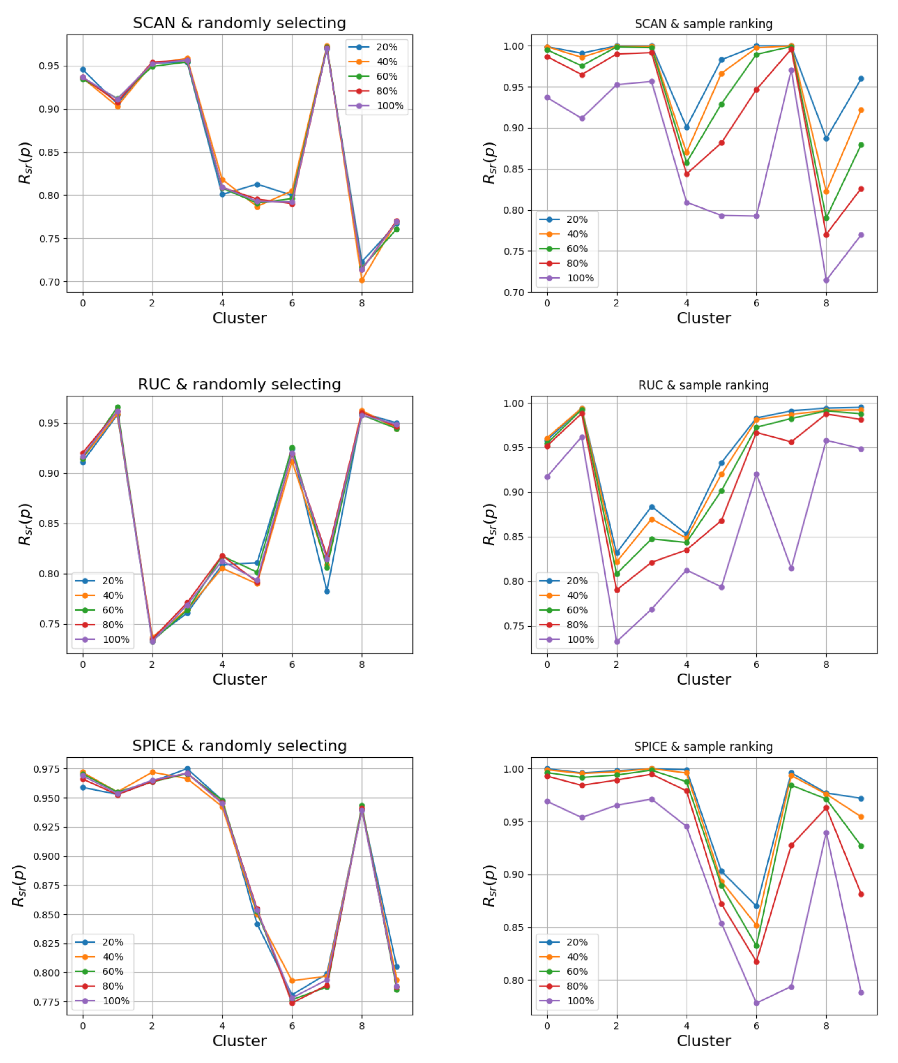
5.1. Performance of Sample Ranking Algorithm

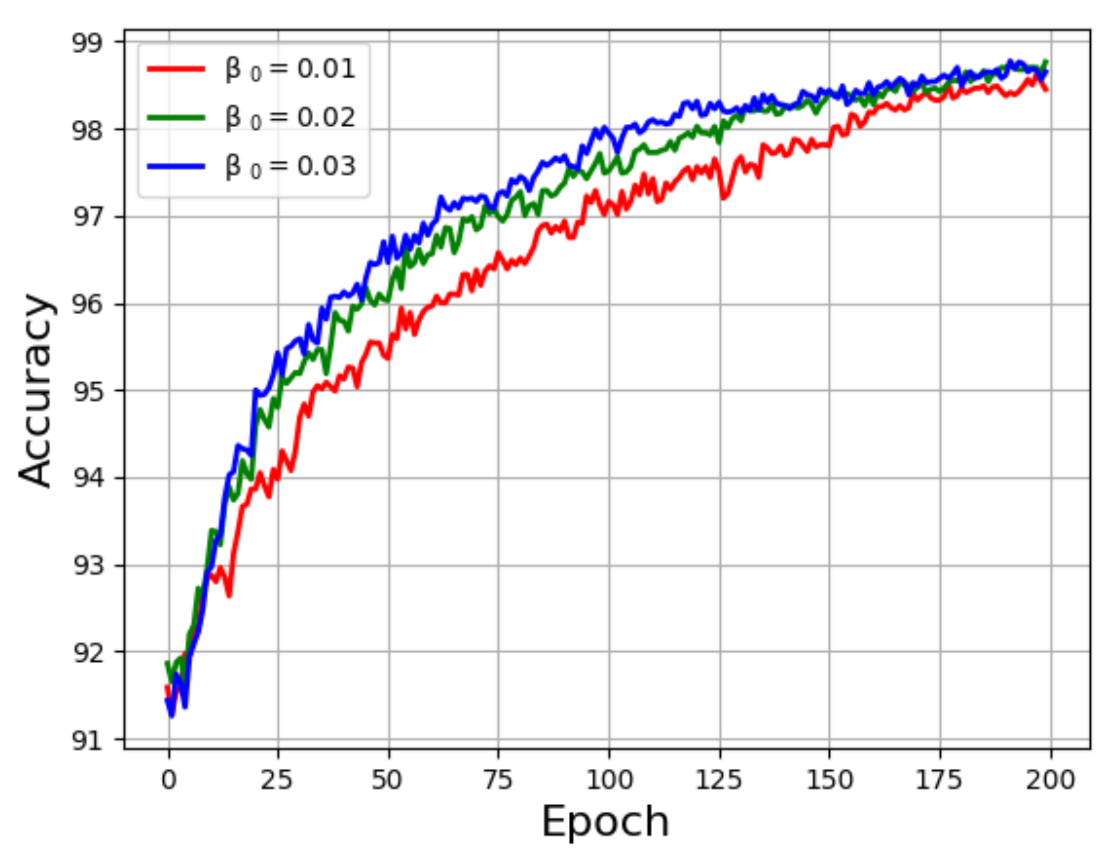
The core of the ICSR technique is the sample ranking and robust majority voting algorithm: Figure 1 and Algorithm 1. ICSR assumes that each cluster has a dominant class, i.e., one class has more samples than other classes, and we call samples from the dominant class as the signal and other samples noise. The objective of the ranking algorithm is to place signal samples at a higher rank than the noise samples. The more signal samples are placed at a higher rank, the better the performances. We define the percentage of signal samples in the top-ranked $p\%$ of all samples in a cluster as the ranking success rate, $R_{sr}\left(p\right)$:

$$R_{sr}\left(p\right)=\frac{S\left(p\right)}{S\left(p\right)+N\left(p\right)}$$

(15)

where $S\left(p\right)$ is the number of signal samples and $N\left(p\right)$ is the number of noise samples at the top $p\%$ of the ranked samples within a cluster. A good ranking performance should have the following characteristics. For a given p, the larger $R_{sr}\left(p\right)$ is, the better. For a given cluster and $p_i<p_j$, $R_{sr}\left(p_i\right)>R_{sr}\left(p_j\right)$. We illustrate the performance of ICSR’s ranking algorithm in Figure 3. The graphs in the first column are consistent with the statistics, i.e., the percentage of signals in the sub-clusters is close to that of the whole cluster. The graphs in the second column demonstrate the effectiveness of our method, where in all three cases, the ranking success rate $R_{sr}\left(p\right)$ of the top $20\%$ is generally higher than that of the top $40\%$; $R_{sr}\left(p\right)$ of the top $40\%$ is higher than that of the top $60\%$, and so on.

To visualize the effectiveness of our ranking algorithm in remote sensing images, we took dataset UCMerced LandUse as an example to illustrate it. Let us focus on one class of remote sensing images, for example the tennis court. In the dataset, all images of tennis court are given in Figure 4.

When we apply the clustering-based representation learning method [30] to UCMerced LandUse, the cluster containing most tennis court images is given in Figure 5. We see that besides tennis court, there are some images of denser residential, building, and so on. There are 101 images in Figure 5, and 71 of them contain a tennis court.

Performing our ranking algorithm, we rank the images in Figure 5 into five groups, as shown in Figure 6. As can be seen from Figure 6, the images in the first, second, and third groups are all correctly clustered. There are still eight images of tennis courts in the fourth group and only three images of tennis courts in the last group. The ranking in Figure 6 is expected: from the first to the last group, the reliability decreased. Other examples are given in Appendix A and Appendix B.

5.2. Ablation Study

The ICSR technique has an important free parameter ${\beta }_0$ in (11), which controls the weights $w_i\left(t\right)$. In the training, we expect that $w_i\left(t\right)$ with $i>1$ gradually increases. One reason for this is for seeking better weights, and another reason is that as training increases clustering accuracy, more samples are clustered correctly; thus, more pseudo labels become more reliable. In this paper, we rank samples in each cluster into five groups, and thus, there are five weights in (9). To investigate the effect of setting ${\beta }_0$, Figure 7 shows the training behaviors for three different values of ${\beta }_0$ on SLT-10 clustering models from SPICE (these accuracies were evaluated only on testing samples and, thus, higher than the accuracy in Table 2). It is seen that although the convergence behaviors of the models varied with different values, they all converged to the same state after 200 epochs, demonstrating that our method is not overly dependent on the selection of the free parameter and different values of the free parameter will lead to similar performances.

In Figure 8, the values of the five weights varied with $\beta$ ($\beta =(1+t){\beta }_0$; see Equation (11)) are given. As expected, $w_1$ always keeps the same value, 1, unaffected by $\beta$, and $w_2>w_3>w_4>w_5$ is always correct for all $\beta$. When $\beta$ is very small, the values of $w_2,w_3,w_4,w_5$ are very close to zero, which approximately only keep the data of the first group. From Figure 8, we see that $w_2$ grows much faster than $w_3,w_4,w_5$ as $\beta$ increases. In the phase that $w_2$ is very larger than $w_3,w_4,w_5$, there are approximately only two groups of data left. Similarly, when $w_3$ grows large enough, there are approximately only three groups of images left. Note that when ${\beta }_0=0.01$, $\beta$ increase from 0.01 to 1, we need 100 epochs, which means that there are many training epochs, which is roughly equivalent to that there are fewer groups of images. In other words, when the number of ranking groups is set as five, assigning weights as Equation (11) roughly includes the cases with group numbers less than five.

From Figure 7, we see that from Epoch 100 to Epoch 200, the three accuracies still increase, which correspond to $\beta$ from 1 to 2, 2 to 4, and 3 to 6, respectively. Note that the values of the five weights increased large enough after $\beta >1$, and thus, the increasing accuracies after epoch 100 imply that the samples or the pseudo labels that are not the most reliable also have made contributions to improve the performance of clustering. Recall that adding the samples or pseudo labels that are not the most reliable to training the model is the essential difference between our method and previous ones, such as SCAN [31], RUC [36], and SPICE [37].

6. Conclusions

Unsupervised image classification is challenging, but very important, as it can make use of abundant unlabeled data. This paper developed an effective image clustering technique that builds on the pretrained clustering models and improves their performances. To develop this approach, we solved the following problems: first of all, how to estimate the likelihoods of the samples belonging to their current clusters; secondly, how to improve the reliability of this estimation; thirdly, how to dynamically determine the contributions of the pseudo labels according to their confidence, which is varied with the training epochs. Based on the statistics, we introduced the quantity M in Equation (5) to measure pseudo labels’ confidence and employed majority voting to enhance the reliability of this measurement. A scheme is then proposed in Equation (11) to weight the cross-entropy loss according to the confidence of the samples. We applied the proposed method to various remote sensing datasets and compared the performance with SOTA methods. Through the results, we found that our method significantly outperforms SOTA methods in most cases. Besides clustering, the methods proposed in this paper could be applied to data denoising or data cleaning, automatic labeling, feature extracting, model pretraining, and so on.

References

1. Goodfellow, I.; Bengio, Y.; Courville, A. Deep Learning; MIT Press: Cambridge, MA, USA, 2016. [Google Scholar]
2. LeCun, Y.; Bengio, Y.; Hinton, G. Deep learning. Nature 2015, 521, 436–444. [Google Scholar] [CrossRef] [PubMed]
3. Bengio, Y.; Courville, A.; Vincent, P. Representation learning: A review and new perspectives. IEEE Trans. Pattern Anal. Mach. Intell. 2013, 35, 1798–1828. [Google Scholar] [CrossRef] [PubMed]
4. Doersch, C.; Gupta, A.; Efros, A.A. Unsupervised Visual Representation Learning by Context Prediction. In Proceedings of the 2015 IEEE International Conference on Computer Vision (ICCV), Santiago, Chile, 7–13 December 2015; pp. 1422–1430. [Google Scholar]
5. Noroozi, M.; Favaro, P. Unsupervised Learning of Visual Representations by Solving Jigsaw Puzzles. In Proceedings of the ECCV, Amsterdam, The Netherlands, 11–14 October 2016; Springer: Berlin/Heidelberg, Germany, 2016; Volume 9910, pp. 69–84. [Google Scholar]
6. Kim, D.; Cho, D.; Yoo, D.; Kweon, I.S. Learning image representations by completing damaged jigsaw puzzles. In Proceedings of the 2018 IEEE Winter Conference on Applications of Computer Vision (WACV), Lake Tahoe, NV, USA, 12–15 March 2018; pp. 793–802. [Google Scholar]
7. Gidaris, S.; Singh, P.; Komodakis, N. Unsupervised Representation Learning by Predicting Image Rotations. In Proceedings of the 6th International Conference on Learning Representations, Vancouver, BC, Canada, 30 April–3 May 2018. [Google Scholar]
8. Kolesnikov, A.; Zhai, X.; Beyer, L. Revisiting self-supervised visual representation learning. In Proceedings of the IEEE/CVF Conference on Computer Vision and Pattern Recognition, Long Beach, CA, USA, 15–20 June 2019; pp. 1920–1929. [Google Scholar]
9. Zhang, R.; Isola, P.; Efros, A.A. Colorful Image Colorization. In Proceedings of the ECCV, Amsterdam, The Netherlands, 11–14 October 2016; Springer: Berlin/Heidelberg, Germany, 2016; Volume 9907, pp. 649–666. [Google Scholar]
10. Larsson, G.; Maire, M.; Shakhnarovich, G. Learning representations for automatic colorization. In Proceedings of the European Conference on Computer Vision, Amsterdam, The Netherlands, 11–14 October 2016; pp. 577–593. [Google Scholar]
11. Wang, X.; Gupta, A. Unsupervised learning of visual representations using videos. In Proceedings of the IEEE International Conference on Computer Vision, Santiago, Chile, 7–13 December 2015; pp. 2794–2802. [Google Scholar]
12. Van den Oord, A.; Li, Y.; Vinyals, O. Representation learning with contrastive predictive coding. arXiv 2018, arXiv:1807.03748. [Google Scholar]
13. Ye, M.; Zhang, X.; Yuen, P.C.; Chang, S.F. Unsupervised embedding learning via invariant and spreading instance feature. In Proceedings of the IEEE/CVF Conference on Computer Vision and Pattern Recognition, Long Beach, CA, USA, 15–20 June 2019; pp. 6210–6219. [Google Scholar]
14. Henaff, O. Data-efficient image recognition with contrastive predictive coding. In Proceedings of the International Conference on Machine Learning, Online, 13–18 July 2020; pp. 4182–4192. [Google Scholar]
15. Tian, Y.; Krishnan, D.; Isola, P. Contrastive Multiview Coding. In Proceedings of the ECCV, Glasgow, UK, 23–28 August 2020; Springer: Berlin/Heidelberg, Germany, 2020; Volume 12356, pp. 776–794. [Google Scholar]
16. He, K.; Fan, H.; Wu, Y.; Xie, S.; Girshick, R. Momentum contrast for unsupervised visual representation learning. In Proceedings of the IEEE/CVF Conference on Computer Vision and Pattern Recognition, Seattle, WA, USA, 13–19 June 2020; pp. 9729–9738. [Google Scholar]
17. Chen, T.; Kornblith, S.; Norouzi, M.; Hinton, G. A simple framework for contrastive learning of visual representations. In Proceedings of the International Conference on Machine Learning, Online, 13–18 July 2020; pp. 1597–1607. [Google Scholar]
18. Henaff, O.J.; Razavi, A.; Doersch, C.; Eslami, S.M.A.; Oord, A.V.d. Data-Efficient Image Recognition with Contrastive Predictive Coding. arXiv 2019, arXiv:1905.09272. [Google Scholar]
19. Hinton, G.E.; Osindero, S.; Teh, Y.W. A fast learning algorithm for deep belief nets. Neural Comput. 2006, 18, 1527–1554. [Google Scholar] [CrossRef]
20. Lee, H.; Grosse, R.; Ranganath, R.; Ng, A.Y. Convolutional deep belief networks for scalable unsupervised learning of hierarchical representations. In Proceedings of the 26th Annual International Conference on Machine Learning, Montreal, QC, Canada, 14–18 June 2009; pp. 609–616. [Google Scholar]
21. Tang, Y.; Salakhutdinov, R.; Hinton, G. Robust boltzmann machines for recognition and denoising. In Proceedings of the 2012 IEEE Conference on Computer Vision and Pattern Recognition, Providence, RI, USA, 16–21 June 2012; pp. 2264–2271. [Google Scholar]
22. Vincent, P.; Larochelle, H.; Lajoie, I.; Bengio, Y.; Manzagol, P.A. Stacked Denoising Autoencoders: Learning Useful Representations in a Deep Network with a Local Denoising Criterion. J. Mach. Learn. Res. 2010, 11, 3371–3408. [Google Scholar]
23. Ren, Z.; Lee, Y.J. Cross-domain self-supervised multi-task feature learning using synthetic imagery. In Proceedings of the IEEE Conference on Computer Vision and Pattern Recognition, Salt Lake City, UT, USA, 18–22 June 2018; pp. 762–771. [Google Scholar]
24. Jenni, S.; Favaro, P. Self-supervised feature learning by learning to spot artifacts. In Proceedings of the IEEE Conference on Computer Vision and Pattern Recognition, Salt Lake City, UT, USA, 18–22 June 2018; pp. 2733–2742. [Google Scholar]
25. Xie, Q.; Dai, Z.; Du, Y.; Hovy, E.; Neubig, G. Controllable invariance through adversarial feature learning. In Proceedings of the Annual Conference on Neural Information Processing Systems 2017, Long Beach, CA, USA, 4–9 December 2017. [Google Scholar]
26. Donahue, J.; Simonyan, K. Large Scale Adversarial Representation Learning. In Proceedings of the NIPS’19: Proceedings of the 33rd International Conference on Neural Information Processing Systems, Vancouver, QC, Canada, 8–14 December 2019; pp. 10541–10551. [Google Scholar]
27. Caron, M.; Bojanowski, P.; Joulin, A.; Douze, M. Deep Clustering for Unsupervised Learning of Visual Features. In Proceedings of the European Conference on Computer Vision (ECCV), Munich, Germany, 8–14 September 2018; Springer: Berlin/Heidelberg, Germany, 2018; Volume 11218, pp. 139–156. [Google Scholar]
28. Huang, J.; Dong, Q.; Gong, S.; Zhu, X. Unsupervised Deep Learning by Neighbourhood Discovery. In Proceedings of the ICML, Long Beach, CA, USA, 9–15 June 2019; Volume 97, pp. 2849–2858. [Google Scholar]
29. Asano, Y.M.; Rupprecht, C.; Vedaldi, A. Self-labelling via simultaneous clustering and representation learning. In Proceedings of the International Conference on Learning Representations 2020 (ICLR 2020), Addis Ababa, Ethiopia, 26–30 April 2020. [Google Scholar]
30. Li, Q.; Li, B.; Garibaldi, J.M.; Qiu, G. On Designing Good Representation Learning Models. arXiv 2021, arXiv:2107.05948. [Google Scholar]
31. Gansbeke, W.V.; Vandenhende, S.; Georgoulis, S.; Proesmans, M.; Gool, L.V. SCAN: Learning to Classify Images Without Labels. In Proceedings of the Computer Vision–ECCV 2020: 16th European Conference, Glasgow, UK, 23–28 August 2020; Springer: Berlin/Heidelberg, Germany, 2020; Volume 12355, pp. 268–285. [Google Scholar]
32. Rosenberg, C.; Hebert, M.; Schneiderman, H. Semi-supervised self-training of object detection models. In Proceedings of the 2005 Seventh IEEE Workshops on Applications of Computer Vision (WACV/MOTION’05), Breckenridge, CO, USA, 5–7 January 2005; Volume 1, pp. 29–36. [Google Scholar]
33. Lee, D.H. Pseudo-label: The simple and efficient semi-supervised learning method for deep neural networks. In Proceedings of the Workshop on Challenges in Representation Learning, Atlanta, GA, USA, 16–21 June 2013; Volume 3, p. 896. [Google Scholar]
34. Xie, Q.; Luong, M.T.; Hovy, E.; Le, Q.V. Self-training with noisy student improves imagenet classification. In Proceedings of the IEEE/CVF Conference on Computer Vision and Pattern Recognition, Seattle, WA, USA, 13–19 June 2020; pp. 10687–10698. [Google Scholar]
35. Sohn, K.; Berthelot, D.; Li, C.L.; Zhang, Z.; Carlini, N.; Cubuk, E.D.; Kurakin, A.; Zhang, H.; Raffel, C. Fixmatch: Simplifying semi-supervised learning with consistency and confidence. arXiv 2020, arXiv:2001.07685. [Google Scholar]
36. Park, S.; Han, S.; Kim, S.; Kim, D.; Park, S.; Hong, S.; Cha, M. Improving Unsupervised Image Clustering With Robust Learning. In Proceedings of the 2021 IEEE/CVF Conference on Computer Vision and Pattern Recognition Workshops (CVPRW), Nashville, TN, USA, 19–25 June 2021; pp. 12278–12287. [Google Scholar]
37. Niu, C.; Wang, G. SPICE: Semantic Pseudo-labeling for Image Clustering. arXiv 2021, arXiv:2103.09382. [Google Scholar]
38. Gong, Z.; Zhong, P.; Hu, W. Diversity in machine learning. IEEE Access 2019, 7, 64323–64350. [Google Scholar] [CrossRef]
39. Settles, B. Active Learning Literature Survey; University of Wisconsin-Madison Department of Computer Sciences: Madiso, WI, USA, 2009. [Google Scholar]
40. Settles, B. Active learning. Synth. Lect. Artif. Intell. Mach. Learn. 2012, 6, 1–114. [Google Scholar]
41. Hearst, M.A.; Dumais, S.T.; Osuna, E.; Platt, J.; Scholkopf, B. Support vector machines. IEEE Intell. Syst. Their Appl. 1998, 13, 18–28. [Google Scholar] [CrossRef] [Green Version]
42. Zhou, Z.H. A brief introduction to weakly supervised learning. Natl. Sci. Rev. 2018, 5, 44–53. [Google Scholar] [CrossRef] [Green Version]
43. Frénay, B.; Verleysen, M. Classification in the presence of label noise: A survey. IEEE Trans. Neural Netw. Learn. Syst. 2013, 25, 845–869. [Google Scholar] [CrossRef]
44. Angluin, D.; Laird, P. Learning from noisy examples. Mach. Learn. 1988, 2, 343–370. [Google Scholar] [CrossRef] [Green Version]
45. Gao, W.; Wang, L.; Zhou, Z.H. Risk minimization in the presence of label noise. In Proceedings of the AAAI Conference on Artificial Intelligence, Phoenix, AZ, USA, 12–17 February 2016; Volume 30. [Google Scholar]
46. Pathak, D.; Kraähenbuähl, P.; Donahue, J.; Darrell, T.; Efros, A.A. Context Encoders: Feature Learning by Inpainting. In Proceedings of the 2016 IEEE Conference on Computer Vision and Pattern Recognition, Las Vegas, NV, USA, 27–30 June 2016; pp. 2536–2544. [Google Scholar]
47. Larsson, G.; Maire, M.; Shakhnarovich, G. Colorization as a Proxy Task for Visual Understanding. In Proceedings of the 2017 IEEE Conference on Computer Vision and Pattern Recognition, Honolulu, HI, USA, 21–26 July 2017; pp. 840–849. [Google Scholar]
48. Mundhenk, T.N.; Ho, D.; Chen, B.Y. Improvements to Context Based Self-Supervised Learning. In Proceedings of the 2018 IEEE Conference on Computer Vision and Pattern Recognition, Salt Lake City, UT, USA, 18–22 June 2018; pp. 9339–9348. [Google Scholar]
49. Noroozi, M.; Vinjimoor, A.; Favaro, P.; Pirsiavash, H. Boosting Self-Supervised Learning via Knowledge Transfer. In Proceedings of the IEEE Conference on Computer Vision and Pattern Recognition (CVPR), 2018, Salt Lake City, UT, USA, 18–22 June 2018; pp. 9359–9367. [Google Scholar]
50. Baldi, P. Autoencoders, Unsupervised Learning, and Deep Architectures. In Proceedings of the ICML Unsupervised and Transfer Learning, Bellevue, WA, USA, 2 July 2012; Volume 27, pp. 37–50. [Google Scholar]
51. Donahue, J.; Krähenbühl, P.; Darrell, T. Adversarial Feature Learning. In Proceedings of the 5th International Conference on Learning Representations, Toulon, France, 24–26 April 2017. [Google Scholar]
52. Jung, H.; Oh, Y.; Jeong, S.; Lee, C.; Jeon, T. Contrastive Self-Supervised Learning With Smoothed Representation for Remote Sensing. IEEE Geosci. Remote Sens. Lett. 2022, 19, 1–5. [Google Scholar] [CrossRef]
53. Ciocarlan, A.; Stoian, A. Ship Detection in Sentinel 2 Multi-Spectral Images with Self-Supervised Learning. Remote Sens. 2021, 13, 4255. [Google Scholar] [CrossRef]
54. Stojnić, V.; Risojević, V. Self-Supervised Learning of Remote Sensing Scene Representations Using Contrastive Multiview Coding. In Proceedings of the 2021 IEEE/CVF Conference on Computer Vision and Pattern Recognition Workshops (CVPRW), Nashville, TN, USA, 19–25 June 2021; pp. 1182–1191. [Google Scholar]
55. Li, H.; Li, Y.; Zhang, G.; Liu, R.; Huang, H.; Zhu, Q.; Tao, C. Global and local contrastive self-supervised learning for semantic segmentation of HR remote sensing images. IEEE Trans. Geosci. Remote Sens. 2022, 60, 1–14. [Google Scholar] [CrossRef]
56. Akiva, P.; Purri, M.; Leotta, M. Self-Supervised Material and Texture Representation Learning for Remote Sensing Tasks. arXiv 2021, arXiv:2112.01715. [Google Scholar]
57. Ayush, K.; Uzkent, B.; Meng, C.; Tanmay, K.; Burke, M.; Lobell, D.; Ermon, S. Geography-Aware Self-Supervised Learning. arXiv 2021, arXiv:2011.09980. [Google Scholar]
58. Dong, H.; Ma, W.; Wu, Y.; Zhang, J.; Jiao, L. Self-Supervised Representation Learning for Remote Sensing Image Change Detection Based on Temporal Prediction. Remote Sens. 2020, 12, 1868. [Google Scholar] [CrossRef]
59. Xu, Y.; Luo, W.; Hu, A.; Xie, Z.; Xie, X.; Tao, L. TE-SAGAN: An Improved Generative Adversarial Network for Remote Sensing Super-Resolution Images. Remote Sens. 2022, 14, 2425. [Google Scholar] [CrossRef]
60. Xie, J.; Girshick, R.; Farhadi, A. Unsupervised deep embedding for clustering analysis. In Proceedings of the International Conference on Machine Learning, New York, NY, USA, 19–24 June 2016; pp. 478–487. [Google Scholar]
61. Chang, J.; Wang, L.; Meng, G.; Xiang, S.; Pan, C. Deep Adaptive Image Clustering. In Proceedings of the 2017 IEEE International Conference on Computer Vision (ICCV) 2017, Venice, Italy, 22–29 October 2017; pp. 5880–5888. [Google Scholar]
62. Caron, M.; Bojanowski, P.; Mairal, J.; Joulin, A. Unsupervised Pre-Training of Image Features on Non-Curated Data. In Proceedings of the ICCV, Seoul, Korea, 27 October–2 November 2019; pp. 2959–2968. [Google Scholar]
63. Ji, X.; Vedaldi, A.; Henriques, J.F. Invariant Information Clustering for Unsupervised Image Classification and Segmentation. In Proceedings of the ICCV, Seoul, Korea, 27 October–2 November 2019; pp. 9864–9873. [Google Scholar]
64. Hu, W.; Miyato, T.; Tokui, S.; Matsumoto, E.; Sugiyama, M. Learning Discrete Representations via Information Maximizing Self-Augmented Training. In Proceedings of the ICML, Sydney, Australia, 6–11 August 2017; pp. 1558–1567. [Google Scholar]
65. Han, S.; Park, S.; Park, S.; Kim, S.; Cha, M. Mitigating embedding and class assignment mismatch in unsupervised image classification. In Proceedings of the Computer Vision–ECCV 2020: 16th European Conference, Glasgow, UK, 23–28 August 2020; pp. 768–784. [Google Scholar]
66. Bachman, P.; Alsharif, O.; Precup, D. Learning with Pseudo-Ensembles. In Proceedings of the NIPS, Montreal, QC, Canada, 8–13 December 2014; Neural Information Processing Systems Foundation: La Jolla, CA, USA, 2014; pp. 3365–3373. [Google Scholar]
67. Sukhbaatar, S.; Bruna, J.; Paluri, M.; Bourdev, L.; Fergus, R. Training convolutional networks with noisy labels. arXiv 2014, arXiv:1406.2080. [Google Scholar]
68. Estévez, P.A.; Tesmer, M.; Perez, C.A.; Zurada, J.M. Normalized mutual information feature selection. IEEE Trans. Neural Netw. 2009, 20, 189–201. [Google Scholar] [CrossRef] [Green Version]
69. Amelio, A.; Pizzuti, C. Is normalized mutual information a fair measure for comparing community detection methods? In Proceedings of the 2015 IEEE/ACM international Conference on Advances in Social Networks Analysis and Mining 2015, Paris, France, 25–28 August 2015; pp. 1584–1585. [Google Scholar]
70. Rand, W.M. Objective criteria for the evaluation of clustering methods. J. Am. Stat. Assoc. 1971, 66, 846–850. [Google Scholar] [CrossRef]
71. Hubert, L.; Arabie, P. Comparing partitions. J. Classif. 1985, 2, 193–218. [Google Scholar] [CrossRef]
72. Vinh, N.X.; Epps, J.; Bailey, J. Information theoretic measures for clusterings comparison: Variants, properties, normalization and correction for chance. J. Mach. Learn. Res. 2010, 11, 2837–2854. [Google Scholar]
73. Krizhevsky, A.; Hinton, G. Learning Multiple Layers of Features from Tiny Images; Technical Report; University of Toronto: Toronto, ON, Canada, 2009. [Google Scholar]
74. Coates, A.; Ng, A.; Lee, H. An analysis of single-layer networks in unsupervised feature learning. In Proceedings of the Fourteenth International Conference on Artificial Intelligence and Statistics, Taoyuan, Taiwan, 13–15 November 2011; pp. 215–223. [Google Scholar]
75. Russakovsky, O.; Deng, J.; Su, H.; Krause, J.; Satheesh, S.; Ma, S.; Huang, Z.; Karpathy, A.; Khosla, A.; Bernstein, M.; et al. Imagenet large scale visual recognition challenge. Int. J. Comput. Vis. 2015, 115, 211–252. [Google Scholar] [CrossRef] [Green Version]
76. MacQueen, J. Some methods for classification and analysis of multivariate observations. In Proceedings of the Fifth Berkeley Symposium on Mathematical Statistics and Probability, Oakland, CA, USA, 1 January 1967; Volume 1, pp. 281–297. [Google Scholar]
77. Ng, A.Y.; Jordan, M.I.; Weiss, Y. On spectral clustering: Analysis and an algorithm. In Proceedings of the Advances in Neural Information Processing Systems, Vancouver, BC, Canada, 9–14 December 2002; pp. 849–856. [Google Scholar]
78. Franti, P.; Virmajoki, O.; Hautamaki, V. Fast agglomerative clustering using a k-nearest neighbor graph. IEEE Trans. Pattern Anal. Mach. Intell. 2006, 28, 1875–1881. [Google Scholar] [CrossRef]
79. Radford, A.; Metz, L.; Chintala, S. Unsupervised representation learning with deep convolutional generative adversarial networks. arXiv 2015, arXiv:1511.06434. [Google Scholar]
80. Zhou, P.; Hou, Y.; Feng, J. Deep adversarial subspace clustering. In Proceedings of the IEEE Conference on Computer Vision and Pattern Recognition, Salt Lake City, UT, USA, 18–22 June 2018; pp. 1596–1604. [Google Scholar]
81. Chang, J.; Guo, Y.; Wang, L.; Meng, G.; Xiang, S.; Pan, C. Deep discriminative clustering analysis. arXiv 2019, arXiv:1905.01681. [Google Scholar]
82. Helber, P.; Bischke, B.; Dengel, A.; Borth, D. Eurosat: A novel dataset and deep learning benchmark for land use and land cover classification. IEEE J. Sel. Top. Appl. Earth Obs. Remote Sens. 2019, 12, 2217–2226. [Google Scholar] [CrossRef] [Green Version]
83. Helber, P.; Bischke, B.; Dengel, A.; Borth, D. Introducing EuroSAT: A Novel Dataset and Deep Learning Benchmark for Land Use and Land Cover Classification. In Proceedings of the IGARSS 2018—2018 IEEE International Geoscience and Remote Sensing Symposium, Valencia, Spain, 22–27 July 2018; pp. 204–207. [Google Scholar]
84. Ma, A.; Zhong, Y.; Zhang, L. Adaptive multiobjective memetic fuzzy clustering algorithm for remote sensing imagery. IEEE Trans. Geosci. Remote Sens. 2015, 53, 4202–4217. [Google Scholar] [CrossRef]
85. Yang, Y.; Newsam, S. Bag-of-visual-words and spatial extensions for land-use classification. In Proceedings of the 18th SIGSPATIAL International Conference on Advances in Geographic Information Systems, San Jose, CA, USA, 2–5 November 2010 2010; pp. 270–279. [Google Scholar]
86. Xia, G.S.; Hu, J.; Hu, F.; Shi, B.; Bai, X.; Zhong, Y.; Zhang, L.; Lu, X. AID: A benchmark data set for performance evaluation of aerial scene classification. IEEE Trans. Geosci. Remote Sens. 2017, 55, 3965–3981. [Google Scholar] [CrossRef] [Green Version]
87. Zhou, W.; Newsam, S.; Li, C.; Shao, Z. PatternNet: A benchmark dataset for performance evaluation of remote sensing image retrieval. ISPRS J. Photogramm. Remote Sens. 2018, 145, 197–209. [Google Scholar] [CrossRef] [Green Version]
88. Cheng, G.; Han, J.; Lu, X. Remote sensing image scene classification: Benchmark and state of the art. Proc. IEEE 2017, 105, 1865–1883. [Google Scholar] [CrossRef] [Green Version]
Figure 1. Schematic of the robust majority voting technique (also see Algorithm 1). The first row is the N c image samples in a cluster c. The following n rows are samples sorted for n different choices of k. Majority voting is then applied to group the samples based on the following procedure. Step 1: Pick the first p 1 samples from each of the n sorted lists and count how many times they appear. The top p 1 samples receiving the most votes (appeared most frequent) are kept to form Group 1, g 1 . Step 2: Follow the same procedure as Step 1, but replace p 1 with p 2 ( p 2 > p 1 ) to obtain the top p 2 samples receiving the most votes, then remove those samples already included in Group 1 to form Group 2, g 2 . Step 3: Follow the same procedure as Step 1, but replace p 1 with p 3 ( p 3 > p 2 > p 1 ) to obtain the top p 3 samples receiving the most votes, then remove those samples already included in previous groups ( g 1 and g 2 ) to form Group 3, g 3 . Subsequent groups can be formed following this pattern, and in total, we can obtain m groups of such samples. It is not difficult to understand that samples in group i will be less likely to be noise than samples in group i + 1 . Samples in the same cluster, but different groups are assigned the same pseudo labels, but differently weighted based on the likelihood of them belonging to noise.
Remotesensing 14 03317 g001
Figure 2. Using the predictions of the network as pseudo labels that could be used to train the network.
Remotesensing 14 03317 g002
Figure 3. Sample ranking performances of Algorithm 1 (see also Figure 1). First column, R s r ( p ) without applying our ranking algorithm and randomly selecting p = 20 % , 40 % , ⋯, 80 % of samples in the clusters formed by 3 pretrained clustering models for CIFAR-10. Second column, after applying our ranking algorithm to rank the samples in the clusters formed by the same 3 pretrained clustering model, R s r ( p ) for p = 20 % , 40 % , ⋯, 80 % .
Remotesensing 14 03317 g003
Figure 4. Ground truth for remote sensing images of tennis courts in UCMerced LandUse. There are 100 images of tennis courts in total.
Remotesensing 14 03317 g004
Figure 5. The remote sensing images of tennis courts clustered by the clustering-based method [30]. There are 101 images in total, and 71 images contain a tennis court.
Remotesensing 14 03317 g005
Figure 6. In the first group, that is the most reliable group of images containing a tennis court, all the images are correctly clustered. The images ranked in the second and third group are also all correctly clustered. In the fourth group, there are 1 image of dense residential, 11 images of mobile home parks, and 8 images of tennis courts. In the last group, there are only 3 images of tennis courts.
Remotesensing 14 03317 g006
Figure 7. Training behaviors of the ICSR technique for different values of the free parameter β 0 on SLT-10 clustering models from SPICE. It is seen that for different selections of the value β 0 , training will converge to almost the same state after 200 epochs.
Remotesensing 14 03317 g007
Figure 8. The values of w 1 , w 2 , w 3 , w 4 , w 5 given by β increases from 0 to 6, where β = ( 1 + t ) β 0 (see Equation (11)).
Remotesensing 14 03317 g008