
Cyclic Global Guiding Network for Point Cloud Completion


Abstract
:
1. Introduction
- We designed the global guided down-sampling and up-sampling constructions. The complete and dense point clouds are reconstructed by combining overall construction with contextual semantic information.
- We integrated the traditional fitting plane of point clouds adapted to point cloud features into the deep learning network, which uses the original features of point clouds to reduce uncertainty.
- We combine a folding operation with an attention mechanism to complete the point cloud by stratification for focusing position creatively.
2. Methods
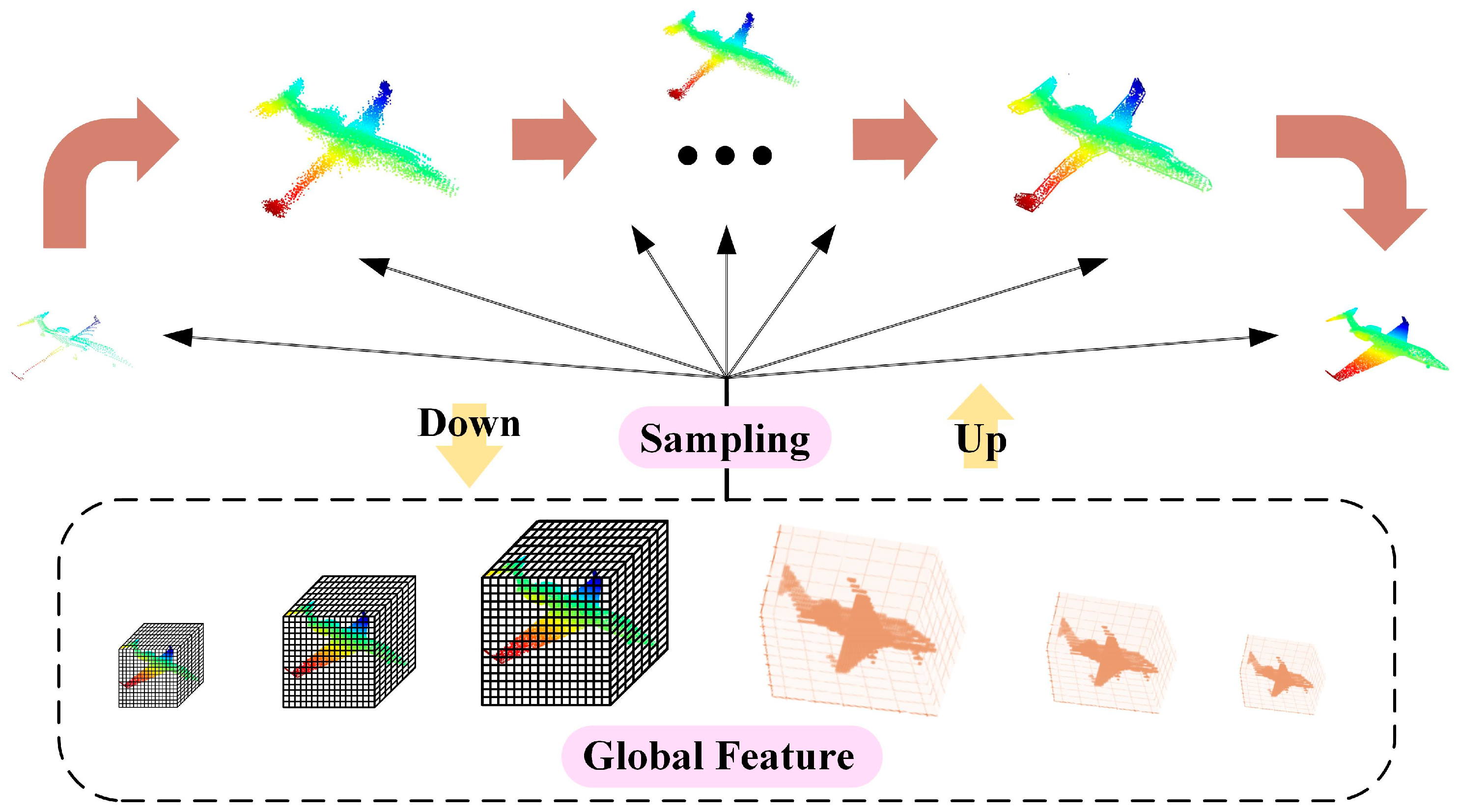
2.1. Global Guided Sampling
2.2. Multiple Fitting Planes
2.3. Layered Folding Attention
2.4. Others
2.4.1. Gridding and Gridding Reverse
2.4.2. Feature Sampling
2.5. Loss Function
3. Results and Discussion
3.1. Results of Comparative Experiments
3.1.1. ShapeNet
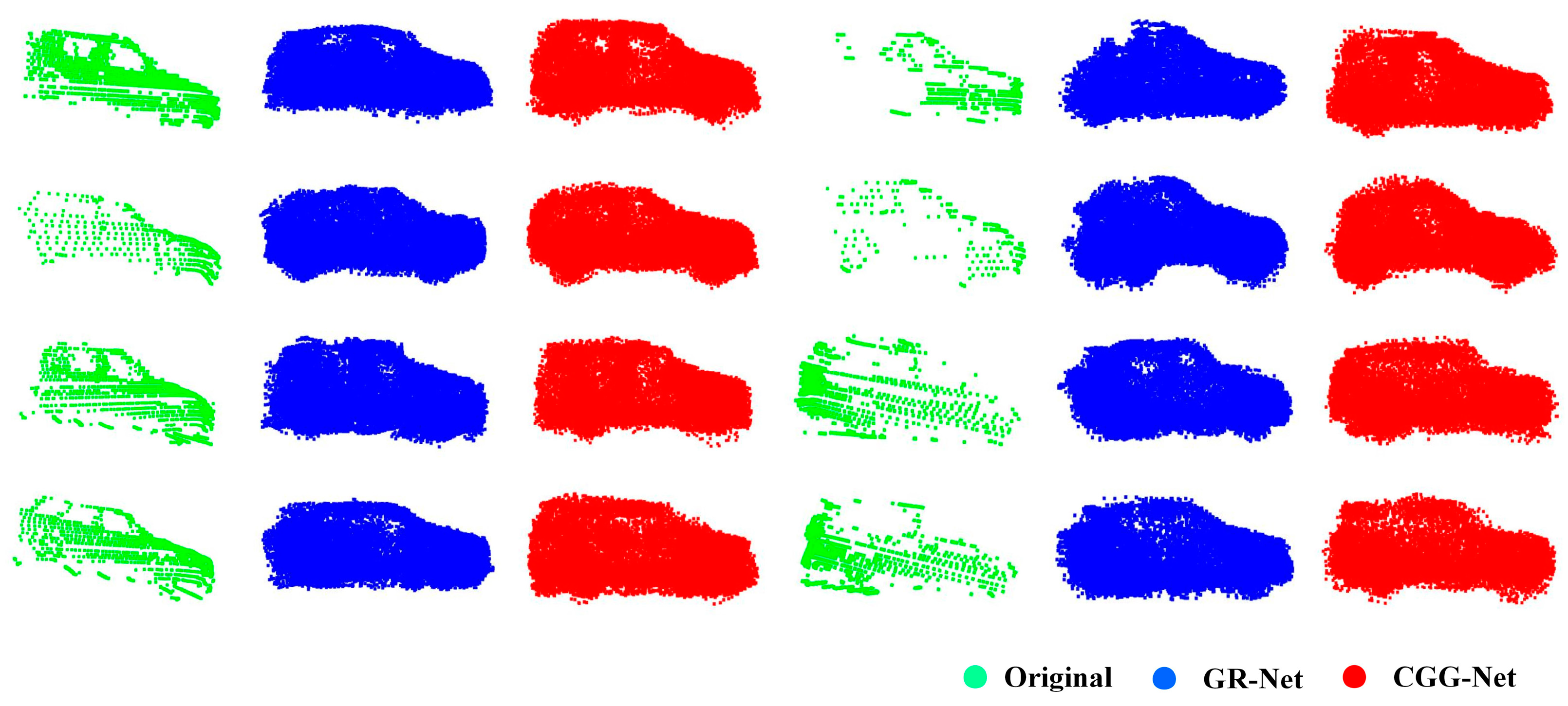
3.1.2. KITTI
3.1.3. MVP
3.2. Results of Ablation Experiments
3.2.1. Global Guided Sampling
3.2.2. Multiple Fitting Planes
3.2.3. Layered Folding Attention
3.2.4. Summary of the Experiment
4. Conclusions
Author Contributions
Funding
Data Availability Statement
Conflicts of Interest
References
- Huang, X.; Zhang, J.; Wu, Q.; Fan, L.; Yuan, C. A Coarse-to-Fine Algorithm for Matching and Registration in 3D Cross-Source Point Clouds. IEEE Trans. Circuits Syst. Video Technol. 2018, 28, 2965–2977. [Google Scholar] [CrossRef] [Green Version]
- Manuele, S.; Gianpaolo, P.; Francesco, B.; Tamy, B.; Paolo, C. High Dynamic Range Point Clouds for Real-Time Relighting. Comput. Graph. Forum 2019, 38, 513–525. [Google Scholar]
- Li, S.; Ye, Y.; Liu, J.; Guo, L. VPRNet: Virtual Points Registration Network for Partial-to-Partial Point Cloud Registration. Remote Sens. 2022, 14, 2559. [Google Scholar] [CrossRef]
- Fan, H.; Su, H.; Guibas, L. A Point Set Generation Network for 3D Object Reconstruction from a Single Image. In Proceedings of the 2017 IEEE Conference on Computer Vision and Pattern Recognition (CVPR), Honolulu, HI, USA, 21–26 July 2017; pp. 2463–2471. [Google Scholar]
- Mittal, H.; Okorn, B.; Jangid, A.; Held, D. Self-Supervised Point Cloud Completion via Inpainting. arXiv 2021, arXiv:2111.10701. [Google Scholar]
- Pan, L.; Chen, X.; Cai, Z.; Zhang, J.; Liu, Z. Variational Relational Point Completion Network. In Proceedings of the 2021 IEEE/CVF Conference on Computer Vision and Pattern Recognition (CVPR), Nashville, TN, USA, 19–25 June 2021; pp. 8520–8529. [Google Scholar]
- Gurumurthy, S.; Agrawal, S. High Fidelity Semantic Shape Completion for Point Clouds Using Latent Optimization. In Proceedings of the 2019 IEEE Winter Conference on Applications of Computer Vision (WACV), Waikoloa Village, HI, USA, 7–11 January 2019; pp. 1099–1108. [Google Scholar]
- Xie, H.; Yao, H.; Zhou, S.; Mao, J.; Sun, W. GRNet: Gridding Residual Network for Dense Point Cloud Completion. In Proceedings of the European Conference on Computer Vision, Glasgow, UK, 23–28 August 2020. [Google Scholar]
- Wen, X.; Li, T.; Han, Z.; Liu, Y. Point Cloud Completion by Skip-Attention Network With Hierarchical Folding. In Proceedings of the 2020 IEEE/CVF Conference on Computer Vision and Pattern Recognition (CVPR), Seattle, WA, USA, 13–19 June 2020; pp. 1936–1945. [Google Scholar]
- Huang, H.; Chen, H.; Li, J. Deep Neural Network for 3D Point Cloud Completion with Multistage Loss Function. In Proceedings of the 2019 Chinese Control And Decision Conference (CCDC), Nanchang, China, 3–5 June 2019; pp. 4604–4609. [Google Scholar]
- Yang, Y.; Feng, C.; Shen, Y.; Tian, D. FoldingNet: Point Cloud Auto-Encoder via Deep Grid Deformation. In Proceedings of the 2018 IEEE/CVF Conference on Computer Vision and Pattern Recognition, Salt Lake City, UT, USA, 18–23 June 2018; pp. 206–215. [Google Scholar]
- Pan, L. ECG: Edge-aware Point Cloud Completion with Graph Convolution. IEEE Robot. Autom. Lett. 2020, 5, 4392–4398. [Google Scholar] [CrossRef]
- Charles, R.Q.; Su, H.; Kaichun, M.; Guibas, L.J. PointNet: Deep Learning on Point Sets for 3D Classification and Segmentation. In Proceedings of the 2017 IEEE Conference on Computer Vision and Pattern Recognition (CVPR), Honolulu, HI, USA, 21–26 July 2017; pp. 77–85. [Google Scholar]
- Charles, R.Q.; Yi, L.; Su, H.; Guibas, L.J. Pointnet++: Deep hierarchical feature learning on point sets in a metric space. Adv. Neural Inf. Process. Syst. 2017, 30, 5105–5114. [Google Scholar]
- Yuan, W.; Khot, T.; Held, D.; Mertz, C.; Hebert, M. PCN: Point Completion Network. In Proceedings of the 2018 International Conference on 3D Vision (3DV), Verona, Italy, 5–8 September 2018; pp. 728–737. [Google Scholar]
- Zhao, Y.; Birdal, T.; Deng, H.; Tombari, F. 3D Point Capsule Networks. In Proceedings of the 2019 IEEE/CVF Conference on Computer Vision and Pattern Recognition (CVPR), Long Beach, CA, USA, 15–20 June 2019; pp. 1009–1018. [Google Scholar]
- Liu, M.; Sheng, L.; Yang, S.; Shao, J.; Hu, S.M. Morphing and Sampling Network for Dense Point Cloud Completion. In Proceedings of the AAAI Conference on Artificial Intelligence, Honolulu, HI, USA, 27 January–1 February 2019. [Google Scholar]
- Tchapmi, L.P.; Kosaraju, V.; Rezatofighi, H.; Reid, I.; Savarese, S. TopNet: Structural Point Cloud Decoder. In Proceedings of the 2019 IEEE/CVF Conference on Computer Vision and Pattern Recognition (CVPR), Long Beach, CA, USA, 15–20 June 2019; pp. 383–392. [Google Scholar]
- Wen, X. PMP-Net: Point Cloud Completion by Learning Multi-step Point Moving Paths. In Proceedings of the 2021 IEEE/CVF Conference on Computer Vision and Pattern Recognition (CVPR), Nashville, TN, USA, 20–25 June 2021; pp. 7439–7448. [Google Scholar]
- Li, R.; Li, X.; Fu, C.W.; Cohen-Or, D.; Heng, P.A. PU-GAN: A Point Cloud Upsampling Adversarial Network. In Proceedings of the 2019 IEEE/CVF International Conference on Computer Vision (ICCV), Seoul, Korea, 20 October–2 November 2019; pp. 7202–7211. [Google Scholar]
- Achlioptas, P.; Diamanti, O.; Mitliagkas, I.; Guibas, L. Learning Representations and Generative Models for 3D Point Clouds. In Proceedings of the 35th International Conference on Machine Learning, Stockholm, Sweden, 10–15 July 2018; pp. 40–49. [Google Scholar]
- Sarmad, M.; Lee, H.J.; Kim, Y.M. RL-GAN-Net: A Reinforcement Learning Agent Controlled GAN Network for Real-Time Point Cloud Shape Completion. In Proceedings of the 2019 IEEE/CVF Conference on Computer Vision and Pattern Recognition (CVPR), Long Beach, CA, USA, 15–20 June 2019; pp. 5891–5900. [Google Scholar]
- Huang, Z.; Yu, Y.; Xu, J.; Ni, F.; Le, X. PF-Net: Point Fractal Network for 3D Point Cloud Completion. In Proceedings of the 2020 IEEE/CVF Conference on Computer Vision and Pattern Recognition (CVPR), Seattle, WA, USA, 13–19 June 2020; pp. 7659–7667. [Google Scholar]
- Xie, C.; Wang, C.; Zhang, B.; Yang, H.; Chen, D.; Wen, F. Style-based Point Generator with Adversarial Rendering for Point Cloud Completion. In Proceedings of the 2021 IEEE/CVF Conference on Computer Vision and Pattern Recognition (CVPR), Nashville, TN, USA, 20–25 June 2021; pp. 4617–4626. [Google Scholar]
- Velikovi, P.; Cucurull, G.; Casanova, A.; Romero, A.; Liò, P.; Bengio, Y. Graph Attention Networks. arXiv 2017, arXiv:1710.10903. [Google Scholar]
- Wang, Y.; Sun, Y.; Liu, Z.; Sarma, S.E.; Bronstein, M.M.; Solomon, J.M. Dynamic Graph CNN for Learning on Point Clouds. ACM Trans. Graph. 2019, 38, 1–12. [Google Scholar] [CrossRef] [Green Version]
- Song, Z.; Zhao, L.; Zhou, J. Learning Hybrid Semantic Affinity for Point Cloud Segmentation. IEEE Trans. Circuits Syst. Video Technol. 2021, 32, 4599–4612. [Google Scholar] [CrossRef]
- Zhang, K.; Hao, M.; Wang, J.; Silva, C.D.; Fu, C. Linked Dynamic Graph CNN: Learning on Point Cloud via Linking Hierarchical Features. arXiv 1904, arXiv:1904.10014. [Google Scholar]
- Wu, W.; Qi, Z.; Fuxin, L. PointConv: Deep Convolutional Networks on 3D Point Clouds. In Proceedings of the 2019 IEEE/CVF Conference on Computer Vision and Pattern Recognition (CVPR), Long Beach, CA, USA, 15–20 June 2019; pp. 9621–9630. [Google Scholar]
- Hua, B.; Tran, M.; Yeung, S. Pointwise Convolutional Neural Networks. In Proceedings of the 2018 IEEE/CVF Conference on Computer Vision and Pattern Recognition, Salt Lake City, UT, USA, 18–23 June 2018; pp. 984–993. [Google Scholar]
- Lei, H.; Akhtar, N.; Mian, A. Octree Guided CNN with Spherical Kernels for 3D Point Clouds. In Proceedings of the 2019 IEEE/CVF Conference on Computer Vision and Pattern Recognition (CVPR), Long Beach, CA, USA, 15–20 June 2019; pp. 9623–9632. [Google Scholar]
- Liu, S.; Fu, K.; Wang, M.; Song, Z. Group-in-Group Relation-Based Transformer for 3D Point Cloud Learning. Remote Sens. 2022, 14, 1563. [Google Scholar] [CrossRef]
- Engel, N.; Belagiannis, V.; Dietmayer, K. Point Transformer. arXiv 2012, arXiv:2012.09164. [Google Scholar] [CrossRef]
- Guo, M.H.; Cai, J.X.; Liu, Z.N.; Mu, T.J.; Martin, R. PCT: Point cloud transformer. Comp. Vis. Media 2021, 7, 187–199. [Google Scholar] [CrossRef]
- Yu, X.; Rao, Y.; Wang, Z.; Liu, Z.; Lu, J.; Zhou, J. PoinTr: Diverse Point Cloud Completion with Geometry-Aware Transformers. arXiv 2021, arXiv:2108.08839. [Google Scholar]
- Sun, T.; Liu, G.; Li, R.; Liu, S.; Zhu, S.; Zeng, B. Quadratic Terms based Point-to-Surface 3D Representation for Deep Learning of Point Cloud. IEEE Trans. Circuits Syst. Video Technol. 2022, 32, 2705–2718. [Google Scholar] [CrossRef]
- Zhang, P.; Wang, X.; Ma, L.; Wang, S.; Kwong, S.; Jiang, J. Progressive Point Cloud Upsampling via Differentiable Rendering. IEEE Trans. Circuits Syst. Video Technol. 2021, 31, 4673–4685. [Google Scholar] [CrossRef]
- Zhang, Z.; Sun, J.; Dai, Y.; Fan, B.; He, M. VRNet: Learning the Rectified Virtual Corresponding Points for 3D Point Cloud Registration. arXiv 2022, arXiv:2203.13241. [Google Scholar] [CrossRef]
- Miao, Y.; Zhang, L.; Liu, J.; Wang, J.; Liu, F. An End-to-End Shape-Preserving Point Completion Network. IEEE Comput. Graph. Appl. 2021, 41, 20–33. [Google Scholar] [CrossRef]
- Zhang, X.; Wang, J.; Wang, T.; Jiang, R. Hierarchical Feature Fusion with Mixed Convolution Attention for Single Image Dehazing. IEEE Trans. Circuits Syst. Video Technol. 2022, 32, 510–522. [Google Scholar] [CrossRef]
- He, K.; Zhang, X.; Ren, S.; Sun, J. Deep Residual Learning for Image Recognition. In Proceedings of the 2016 IEEE Conference on Computer Vision and Pattern Recognition (CVPR), Las Vegas, NV, USA, 27–30 June 2016; pp. 770–778. [Google Scholar]
- Shi, J.; Xu, L.; Heng, L.; Shen, S. Graph-Guided Deformation for Point Cloud Completion. IEEE Robot. Autom. Lett. 2021, 6, 7081–7088. [Google Scholar] [CrossRef]
- Tatarchenko, M.S.; Richter, R.; Ranftl, R.; Li, Z.; Koltun, V.; Brox, T. What Do Single-View 3D Reconstruction Networks Learn? In Proceedings of the 2019 IEEE/CVF Conference on Computer Vision and Pattern Recognition (CVPR), Long Beach, CA, USA, 15–20 June 2019; pp. 3400–3409. [Google Scholar]
- Groueix, T.; Fisher, M.; Kim, V.G.; Russell, B.C.; Aubry, M. AtlasNet: A Papier-Mché Approach to Learning 3D Surface Generation. In Proceedings of the IEEE Conference on Computer Vision and Pattern Recognition (CVPR), Salt Lake City, UT, USA, 18–23 June 2018. [Google Scholar]
- Geiger, A.; Lenz, P.; Stiller, C.; Urtasun, R. Vision meets robotics: The KITTI dataset. Int. J. Robot. Res. 2013, 32, 1231–1237. [Google Scholar] [CrossRef] [Green Version]


| Model | F-Net | Top-Net | MSN | GR-Net | Spare-Net | CGG-Net |
|---|---|---|---|---|---|---|
| Airplane | 0.62 | 0.22 | 0.25 | 0.29 | 0.18 | 0.27 |
| Cabinet | 1.61 | 0.56 | 0.97 | 0.63 | 0.66 | 0.59 |
| Car | 0.62 | 0.35 | 0.45 | 0.32 | 0.36 | 0.31 |
| Chair | 1.55 | 0.63 | 0.77 | 0.55 | 0.62 | 0.54 |
| Lamp | 2.03 | 0.75 | 0.93 | 0.58 | 0.63 | 0.38 |
| Sofa | 1.54 | 0.69 | 1.15 | 0.69 | 0.79 | 0.76 |
| Table | 1.53 | 0.48 | 0.67 | 0.48 | 0.50 | 0.41 |
| Watercraft | 0.91 | 0.44 | 0.49 | 0.31 | 0.38 | 0.29 |
| Overall | 1.30 | 0.52 | 0.71 | 0.48 | 0.52 | 0.44 |
| Model | GAN | CD | FS | Time |
|---|---|---|---|---|
| Spare-Net | √ | 0.52 | 0.6607 | 1.055 |
| GR-Net | × | 0.48 | 0.6179 | 0.020 |
| CGG-Net | × | 0.44 | 0.6266 | 0.022 |
| Datasets | Percentage | Atlas-Net | PCN | F-Net | Top-Net | MSN | GR-Net | CGG-Net |
|---|---|---|---|---|---|---|---|---|
| ShapeNet-Car | 0.6% | - | - | - | - | - | 0.23 | 0.12 |
| 0.8% | - | - | - | - | - | 0.14 | 0.11 | |
| 1.0% | - | - | - | - | - | 0.08 | 0.07 | |
| 1.2% | - | - | - | - | - | 0.05 | 0.04 | |
| KITTI | 0.6% | 1.01 | 5.81 | 1.30 | 1.32 | 0.68 | 0.27 | 0.27 |
| 0.8% | 0.87 | 7.71 | 1.26 | 1.22 | 0.52 | 0.20 | 0.19 | |
| 1.0% | 0.76 | 9.33 | 1.16 | 1.07 | 0.46 | 0.15 | 0.13 | |
| 1.2% | 0.69 | 10.82 | 1.06 | 0.95 | 0.38 | 0.12 | 0.10 |
| Model | CD_t | CD_p | FS | |
|---|---|---|---|---|
| MLP tree-based | TOP-Net | 1.915 | 0.120 | 0.299 |
| 3D Conv-based | GR-Net | 1.871 | 0.172 | 0.377 |
| CGG-Net | 1.718 | 0.143 | 0.398 |
| Categories/ Model | Air-Plane | Cabinet | Car | Chair | Lamp | Sofa | Table | Water-Craft | Overall | |
|---|---|---|---|---|---|---|---|---|---|---|
| CD (Lower is better) | None | 0.28 | 0.60 | 0.33 | 0.49 | 0.51 | 0.98 | 0.45 | 0.32 | 0.50 |
| Add | 0.27 | 0.58 | 0.35 | 0.56 | 0.41 | 0.84 | 0.43 | 0.30 | 0.47 | |
| FS (Higher is better) | None | 0.77 | 0.51 | 0.60 | 0.58 | 0.69 | 0.48 | 0.64 | 0.69 | 0.61 |
| Add | 0.78 | 0.51 | 0.60 | 0.58 | 0.69 | 0.49 | 0.65 | 0.70 | 0.62 |
| Categories | CD (Lower Is Better) | |
|---|---|---|
| None | Add | |
| Airplane | 0.27 | 0.29 |
| Cabinet | 0.58 | 0.63 |
| Car | 0.35 | 0.32 |
| Chair | 0.56 | 0.53 |
| Lamp | 0.42 | 0.42 |
| Sofa | 0.84 | 0.65 |
| Table | 0.43 | 0.46 |
| Watercraft | 0.30 | 0.30 |
| Overall | 0.47 | 0.46 |
| Categories/ Model | Airplane | Cabinet | Car | Chair | Lamp | Sofa | Table | Watercraft | Overall | |
|---|---|---|---|---|---|---|---|---|---|---|
| CD (Lower is better) | None | 0.29 | 0.63 | 0.32 | 0.53 | 0.42 | 0.65 | 0.46 | 0.30 | 0.46 |
| 16 | 0.29 | 0.56 | 0.35 | 0.51 | 0.41 | 0.78 | 0.48 | 0.29 | 0.46 | |
| 32 | 0.27 | 0.59 | 0.31 | 0.54 | 0.38 | 0.76 | 0.41 | 0.29 | 0.44 | |
| 64 | 0.24 | 0.55 | 0.32 | 0.55 | 0.39 | 0.78 | 0.57 | 0.30 | 0.46 | |
| FS (Higher is better) | None | 0.78 | 0.52 | 0.60 | 0.59 | 0.70 | 0.49 | 0.65 | 0.70 | 0.62 |
| 16 | 0.77 | 0.51 | 0.60 | 0.58 | 0.69 | 0.48 | 0.64 | 0.69 | 0.62 | |
| 32 | 0.79 | 0.53 | 0.61 | 0.59 | 0.70 | 0.50 | 0.66 | 0.70 | 0.64 | |
| 64 | 0.78 | 0.52 | 0.60 | 0.58 | 0.70 | 0.49 | 0.65 | 0.69 | 0.63 |
| Model | CD | FS | Weights (M) | Time (s) |
|---|---|---|---|---|
| Original | 0.50 | 0.61 | 306.8 | 0.019 |
| Original+GGS | 0.47 | 0.62 | 307.0 | 0.020 |
| Original+GGS+MFP | 0.46 | 0.62 | 321.5 | 0.020 |
| Original+GGS+MFP+LFA-16 | 0.46 | 0.62 | 338.3 | 0.022 |
| Original+GGS+MFP+LFA-32 | 0.44 | 0.64 | 338.3 | 0.022 |
| Original+GGS+MFP+LFA-64 | 0.46 | 0.63 | 338.3 | 0.022 |
Publisher’s Note: MDPI stays neutral with regard to jurisdictional claims in published maps and institutional affiliations. |
© 2022 by the authors. Licensee MDPI, Basel, Switzerland. This article is an open access article distributed under the terms and conditions of the Creative Commons Attribution (CC BY) license (https://creativecommons.org/licenses/by/4.0/).
Share and Cite
Wei, M.; Zhu, M.; Zhang, Y.; Sun, J.; Wang, J. Cyclic Global Guiding Network for Point Cloud Completion. Remote Sens. 2022, 14, 3316. https://doi.org/10.3390/rs14143316
Wei M, Zhu M, Zhang Y, Sun J, Wang J. Cyclic Global Guiding Network for Point Cloud Completion. Remote Sensing. 2022; 14(14):3316. https://doi.org/10.3390/rs14143316
Chicago/Turabian StyleWei, Ming, Ming Zhu, Yaoyuan Zhang, Jiaqi Sun, and Jiarong Wang. 2022. "Cyclic Global Guiding Network for Point Cloud Completion" Remote Sensing 14, no. 14: 3316. https://doi.org/10.3390/rs14143316
APA StyleWei, M., Zhu, M., Zhang, Y., Sun, J., & Wang, J. (2022). Cyclic Global Guiding Network for Point Cloud Completion. Remote Sensing, 14(14), 3316. https://doi.org/10.3390/rs14143316