
Improving Satellite Retrieval of Coastal Aquaculture Pond by Adding Water Quality Parameters


1
Center for Water Resources and Environment, School of Civil Engineering, Sun Yat-sen University, Guangzhou 510275, China
2
Southern Marine Science and Engineering Guangdong Laboratory, Zhuhai 519082, China
3
Department of Global Ecology, Carnegie Institution for Science, Stanford, CA 94305, USA
*
Author to whom correspondence should be addressed.
Remote Sens. 2022, 14(14), 3306; https://doi.org/10.3390/rs14143306
Submission received: 18 May 2022
/
Revised: 19 June 2022
/
Accepted: 4 July 2022
/
Published: 8 July 2022
(This article belongs to the Special Issue Remote Sensing for Agricultural, Environmental and Forestry Policies)
Abstract
:Coastal aquaculture is an important supply of animal proteins for human consumption, which is expanding globally. Meanwhile, extensive aquaculture may increase nutrient loadings and environmental concerns along the coast. Accurate information on aquaculture pond location is essential for coastal management. Traditional methods use morphological parameters to characterize the geometry of surface waters to differentiate artificially constructed conventional aquaculture ponds from other water bodies. However, there are other water bodies with similar morphology (e.g., saltworks, rice fields, and small reservoirs) that are difficult to distinguish from aquaculture ponds, causing a lot of omission/commissioning errors in areas with complex land-use types. Here, we develop an extraction method with shape and water quality parameters to map aquaculture ponds, including three steps: (1) Sharpen normalized difference water index to detect and binarize water pixels by the Otsu method; (2) Connect independent water pixels into water objects through the four-neighbor connectivity algorithm; and (3) Calculate the shape features and water quality features of water objects and input them into the classifier for supervised classification. We selected eight sites along the coast of China to evaluate the accuracy and generalization of our method in an environment with heterogeneous pond morphology and landscape. The results showed that six transfer characteristics including water quality characteristics improved the accuracy of distinguishing aquaculture ponds from salt pans, rice fields, and wetland parks, which typically had F1 scores > 85%. Our method significantly improved extraction efficiency on average, especially when aquaculture ponds are mixed with other morphological similar water bodies. Our identified area was in agreement with statistics data of 12 coastal provinces in China. In addition, our approach can effectively improve water objects when high-resolution remote sensing images are unavailable. This work was applied to open-source remote sensing imagery and has the potential to extract long-term series and large-scale aquaculture ponds globally.
1. Introduction
Fish products, rich in nutrients, are indispensable foods for human beings. According to the Food and Agriculture Organization of the United Nations, food fish consumption per capita grew from 9.0 kg to 20.5 kg in the past 50 years [1,2]. Aquaculture is an important way to meet people’s demand for fish products and has undoubtedly become the fastest-growing food production sector in the world [3,4]. The coastal aquaculture industry has been one of the most dynamic growth sectors over the past 20 years for reasons such as addressing employment, developing the economy, and eradicating poverty [5,6]. Expansion of aquaculture ponds has been found along the coastline worldwide [7,8,9,10,11,12,13,14,15,16].
Coastal aquaculture ponds have been detected by remote sensing images at different scales [17,18,19,20]. The most common approach is to use characteristics of water objects extracted from remote sensing imagery to identify these ponds. Extraction of water objects typically consists of two steps: (1) creating connected features and (2) extracting water objects. The single-band images are used to generate a set of non-overlapping homogeneous segments (polygons) after using a threshold to mask unnecessary pixels [21]. These homogeneous segments (polygons) are calculated as connected features by a connecting algorithm to generate objects for classification [22]. However, the object-based method is hindered by the presence of mixed pixels. One example, the width of pathways between two aquaculture ponds generally does not exceed 5 m, and the presence of pathways results in mixed pixels that have a coarser resolution than 5 m [20]. Such mixed pixels lead to the omission and commission errors of water objects [17]. Disperati et al. (2015) [23] showed that the application of object-based supervised classification can distinguish aquaculture ponds from other water bodies. Ren et al. (2019) [18] used the object-based image analysis (OBIA) function of eCognition Developer 64 software (based on the region growth algorithm [24,25]), and then analyzed the expansion of aquaculture ponds along the coast of China from 1984 to 2016. The results suggested that the Yangtze River Delta, the Pearl River Delta, and the Bohai Bay have been the hotspots of rapid aquaculture expansion over the past 30 years. Ottinger et al. (2017) [26] used the sentinel-1 VH band to extract aquaculture ponds based on the frequent filling feature and geometry. In these studies, image binary segmentation and connecting algorithms were used to create water objects [19], and the classification results usually depend on specific parameters (e.g., perimeter, area, and compactness), which may be difficult to reuse and reproduce for large scale applications.
The selection of key geomorphological parameters is critical to identify water objects as targeting water bodies. Zeng et al. (2019) [20] used medium-resolution remote sensing images and the curvature of an artificial pond with a regular boundary as a classification feature to extract aquaculture ponds around inland lakes. Duan et al. (2020) [27] established a decision tree model based on the Google Earth Engine (GEE) platform open-source race Landsat7 data via shape and convolution operations. The extracted results revealed the growth rate of aquaculture in Jiangsu, China. These geomorphological parameters can selectively capture aquaculture ponds according to local characteristics. For example, in coastal regions with low drainage density (e.g., North China), the shape of aquaculture ponds is regular. Saltworks [18] and segmented rivers [28] are similar to aquaculture ponds in terms of morphological characteristics, which can hardly be distinguished from each other. In addition, due to dense river networks and a large number of fragmented water bodies, the shape of ponds is irregular in South China, and aquaculture ponds can be confused with small water bodies in wetlands. Practically, it is still challenging to differentiate small-scale water bodies, paddy fields [29], and aquaculture ponds using traditional approaches.
Recent progress in water quality remote sensing has shown that water quality parameters, such as chlorophyll-A, colored dissolved organic matter, turbidity, total phosphorus, total nitrogen, and heavy metal pollution can be detected by satellite images (e.g., from Landsat, Sentinel, and MODIS). Water quality parameters indicate the health of a water body and the potential risks of fish and other aquatic organisms [30], and are used as important parameters in limnology and oceanography to evaluate the nutritional status and ecological health of the aquatic environment [31]. Since aquaculture heavily relies on water quality (e.g., dissolved oxygen, ammonia nitrogen, and nitrite) to maintain the optimal growth conditions for fish products to ensure the best yield [32], it may be an effective approach to using water quality parameters in the extraction of aquaculture ponds.
This study investigated the incorporation of water quality parameters to optimize the extraction of aquaculture ponds. We used an object-based method to select a series of shape and water quality parameters and applied the random forest method to evaluate the importance of these parameters. We selected the coast of China as an example to develop and test our methods since China’s aquaculture has developed rapidly. Our goal is to (i) test the usefulness of adding water quality characteristics in aquaculture pond extraction, (ii) develop a new method in aquaculture pond extraction with large area applicability, and (iii) test our method along the coast of China to reveal the expansion of aquaculture. These results have important implications for the extraction of aquaculture ponds and the management of aquatic ecosystems in coastal areas globally. All acronyms used in the paper are given in Table 1.
2. Materials and Methods
2.1. Study Area
Our study area was the 50 km buffer zone from the coast of China (Figure 1). The landscape in coastal areas of China shows a spatial variability from the north to the south [33]. In the north, coastal areas are low elevation plains (≤200 m) featured with regular and large aquaculture ponds (Figure 2f). In the south, the drainage system is well-developed in tropical and subtropical climates. The aquaculture ponds are irregularly distributed along the numerous waterways, and the average area of each pond varies dramatically according to local terrain (Figure 2b). Therefore, we considered the shape, location, area of the aquaculture ponds, and the complexity of the water body types. To test if adding water quality parameters can efficiently improve the identification of aquaculture ponds, we chose 8 sites with diverse types of water bodies covering North and South China. For the convenience of representation, we use regions of interest (ROI) 1–8 in Table 2 to correspond to each site in order.
The test sites in Figure 2a–d are located in South China.
- Donghai Island, Zhanjiang City, Guangdong Province (Figure 2d): extensive aquaculture pond system built on the tidal flats of small straits: irregular shape, large boundary curvatures, and the area of each pond vary dramatically.
- Gulao Water Town, Heshan City, Guangdong Province (Figure 2c): a typical intensive aquaculture system with a river tourism industry across the main river. These ponds naturally developed according to the meandering rivers. Furthermore, the water supply system and pathway are intertwined with aquaculture ponds for tourism. These characteristics increased difficulties in teasing out aquaculture ponds only.
- Wukan Port, Lufeng City, Guangdong Province (Figure 2b): a semi-intensive aquaculture system based on reclaimed bays: ponds are approximately rectangular, and have wide ranges in area variability. Reeds field around the pond is a factor that confuses the aquaculture ponds extraction other than ditches (Field survey photos: Figure S1).
- Pubagang Town, Taizhou City, Zhejiang Province (Figure 2a): a natural aquaculture system on the coastline. Pathways and channels are built to introduce seawater for aquaculture, and the water quality is similar to that of seawater. Some ponds have an irregular shape, which was constrained by the natural coastline.The test site in Figure 2e–h is located in North China.
- Rudong County, Nantong City, Jiangsu Province (Figure 2e): a coastal industrialized intensive aquaculture system. These ponds are rectangular, have close sizes, and are managed uniformly. A modern water purification system is used to balance the nutrient content in the pond water (Field survey photos: Figure S2).
- Chengkou Saltworks, Binzhou City (Figure 2g), Shandong Province: an intensive aquaculture system with both fish ponds and saltworks. The geometry and area of the evaporation ponds and crystallization ponds are similar to those of aquaculture ponds. In addition, the ponds were next to river banks, with irregular shapes (Field survey photos: Figure S4).
- Tianjin Hangu Saltworks (Figure 2h): a coastal aquaculture system next to saltworks. Large area ponds are restricted by coastlines and saltworks. The shape is not regular rectangles, and the curvature of the boundary is high. The salt farm and the aquaculture pond are jointly operated here (Field survey photos: Figure S5).
Each site has its own difficulties, which confuse aquaculture ponds and other water bodies (Table 2).
2.2. Data Collection
2.2.1. Satellite Datasets
The Sentinel-2 Multispectral Instrument (MSI) samples 13 spectral bands: visible and NIR at 10 m, red edge and SWIR at 20 m, and atmospheric bands at 60 m spatial resolution [34]. Its high-resolution multispectral products have been widely used in mapping water bodies and water quality inversion [35]. The Google Earth Engine platform [36] provided all-weather radar images and high-resolution optical images from Sentinel 2. The mapping of aquaculture ponds is generally performed once a year, as aquaculture ponds are generally filled with water throughout the year. We calculated the median per pixel for all Sentinel-2 MSI images over the March to November period each year. Since aquaculture ponds are mostly full of water during this period, the median can characterize the spectral reflectance of the water surface over a long-term series. The band and spatial resolution information of the Sentinel-2 MSI image are listed in Table 3. Moreover, the number of images used every year and the availability of the image is shown in Figures S6 and S7.
2.2.2. Validation Datasets
We used GEE’s random point function to generate 1000 random points in the eight test sites and took the water objects corresponding to the random points as training samples. Aquaculture ponds are usually closed reservoirs artificially constructed or transformed from natural water bodies. We referred to the optical high-resolution images to determine the attributes of the water bodies corresponding to random points (aquaculture or non-aquaculture). To balance the number between the two types of samples (aquaculture or non-aquaculture), we used an oversampling method: the samples of the minority class were repeatedly sampled multiple times. This balances the numbers between the two classes of samples (aquaculture or non-aquaculture), since random forests are sensitive to large numbers of differences between sample classes. The categories of water objects in each dataset were verified by communicating with the local residents. In addition, some water objects were confirmed during field surveys in Wukan Port, Rudong county, Donggang, Chengkou, and Tianjian Hangu Saltworks during the winter and summer of 2021.
2.3. Methods
2.3.1. Water-Object Extraction
We used the object-based method that comprehensively considers the adaptive imagery binarization threshold so that the connectivity algorithm could combine water pixels into a homogeneous water object [21]. First, the Normalized Difference Water Index (NDWI; Equation (1)) [37] was used to distinguish water from non-water:
where Band3 and Band8 represent the Green and Near-infrared bands of Sentinel-2 MSI imagery.
Second, we applied a 3 × 3 high-pass filter (Equation (2)) to sharpen the NDWI image (Figure 3a), which could enhance the contrast between pathway pixels and pond pixels (Figure 3b) [38]. Figure 3g,h suggested that the sharpening filter enabled a more prominent bimodal histogram of NDWI imagery gray values. Third, we used the Otsu method to classify the image [39]. The sharpening filter did not significantly affect the adaptive binarization threshold of the NDWI image. Under the same binarization threshold, the pathway pixels marked as “non-water” in the sharpened image were more distinct (Figure 3c,d). In the end, we applied the “connected components” four-neighbor connectivity function in GEE to the binarized image to obtain the water object (Figure 3e,f).
The water object produced by the sharpened NDWI images had a higher degree of separation and coverage when the pond did not mix with surrounding rivers (Figure 3f). The maximum connection range of the GEE communication function is 1024 pixels. If the mixed pixels due to pathways were incorrectly classified as water, a large portion of aquaculture ponds would be missing (Figure 3e). The high-quality water object increased the ability to project real water bodies, including morphological features and water quality parameters. Moreover, the MNDWI (Based on Sentinel-2 MSI) and Sentinel-1 VH bands were also tested to create water objects. Although these two indicators were sensitive to water and non-water land types as well, we chose the NDWI method according to its performance (see Support text 1 and Figure S8).
2.3.2. Classification Parameter Selection
First, we selected five shape parameters for the water object: Area, Perimeter, Compactness ratio C, Aspect Ratio, and Landscape Shape Index (LSI). The Area and Perimeter of the water object are the most basic morphological parameters. Compactness ratio C is a dimensionless constant in the interval [0, 1], which can effectively distinguish artificial water bodies from natural water bodies. The larger value of Compactness ratios C indicates a more complicated shape [40]; the Aspect Ratio is calculated based on the circumscribed rectangle of the object [41], and the value of aquaculture ponds is generally greater than 1. Likewise, Landscape Shape Index (LSI) is a quantitative measure of landscape complexity or heterogeneity. In general, more complex landscapes have larger perimeters or edges for a given area and therefore a higher LSI [42].
We selected 5 common water quality parameters: Normalized Difference Chlorophyll Index (NDCI), Phycocyanin (2BDA), Maximum Chlorophyll Index (MCI), Colored Dissolved Organic Matter (CDOM), and Surface Algal Bloom Index (SABI). Chl and PC reflect the trophic status of a water body. PC contains a distinct spectral absorption feature centered on 620 nm, and Chl corresponds to 685 nm. To make the PC compatible with Sentinel-2 MSI, Johansen et al. (2019) [43] simplified the empirical equation for the inversion of phycocyanin proposed by Wynne (2008) [44] with the ratio of the red band and the VRE5 band. We chose two indicators that reflect the chlorophyll concentration. The first one was the normalized difference chlorophyll index proposed by Mishra et al. (2012) [45], which is often used to predict the chlorophyll concentration in turbid coastal waters. The other was the Maximum Chlorophyll Index (MCI) [46] based on the fluorescence height baseline algorithm. Here, we used 705 nm as the fluorescent line. As the concentration of colored dissolved organic matter increases, the color of water also changed from dark green to brownish brownish-yellower [47], which was an effective indicator to distinguish natural water bodies from aquaculture ponds. Kutser et al. (2005) [48] mapped the CDOM value through the power function of the ratio of ALI band 2 (565 nm) and band 3 (660 nm). Accordingly, we applied the green (560 nm) and red (665 nm) bands of Sentinel-2 MSI to the power function to predict the CDOM concentration. Similarly, we also included SABI, which can directly detect the spatial distribution of surface and near-surface algae [49]. All shape and water quality parameters are listed in Table 4.
2.3.3. Classification Model Settings and Validation
We used the classification and regression tree model (CART) in a random forest (RF) classifier to extract the aquaculture pond and return the optimized parameter combination [51]. As an ensemble classifier, random forest has the advantages of better accuracy, strong ability to resist the noise of training data, and strong resistance to overfitting. It has been widely used to map land-use types in remote sensing data [52,53]. For building an RF classifier, the Number of Trees (Ntree) and the number of variable divisions (Mtry) are the two most sensitive variables. An increase in the Ntree value does not carry the risk of overfitting, and 500 is usually an acceptable value [54]. Considering that GEE has a computational memory limit, we choose 400, which can achieve a similar effect to 500 and save computational memory. The Mtry parameter is usually set to the square root of the number of input variables [28].
We randomly divided the basic sample dataset of each site into a training dataset and a test dataset, of which the training dataset accounted for 70% and the test dataset accounted for 30%. Such random splits were repeated 10,000 times in the base dataset at each site and fed into a random forest classifier for cross-validation. The purpose of this step is to reveal the effect of adding water quality parameters on the performance and stability of the aquaculture pond classifier.
Firstly, we selected 5 morphological parameters as the control feature combination 1—shape feature combination (SF), because shape parameters are the most commonly used classification features for classifying aquaculture ponds. Secondly, set three experimental feature combinations: experimental feature combination 1—water quality parameter feature combination (WQF); experimental feature combination 2—mixed feature recursive feature elimination (MFRFE); experimental feature combination 3—mixed feature non-recursive feature elimination (MFNRFE).
The experimental feature combination has the same number of parameters as the control feature combination. In addition, in each cross-validation, the random forest classifier can sort the importance of all morphological parameters (5 in total) and water quality parameters (5 in total) according to the GINI index, eliminating unimportant features to save computing memory and improve the classification accuracy. There are two main methods of feature elimination, feature recursive feature elimination and feature non-recursive feature elimination. The details of these two methods are mentioned in Guyon et al. (2003) [55]. Experimental feature combinations 2 and 3 are obtained by different elimination strategies.
The core of accuracy evaluation is the confusion matrix [56,57]. Some measures of the consistency between evaluation model predictions and actual surveys are proposed by the confusion matrix [58], user’s accuracy (UA), producer’s accuracy (PA):
Ni: represents the amount of sample data of class i. N:j represents the amount of class j in the prediction result of the model. PA represents the probability that a pixel is correctly classified, and reflects the reliability of a certain type of prediction. UA represents the probability that the classified pixels represent the class, reflecting the correct attribution of a certain class of sample data. These two measures evaluate whether the model is biased to correctly classify the majority class, resulting in a low accuracy rate for the minority class [56]. Helldén (1980) [59] developed a harmonic average of producer and user accuracy, called the average accuracy index. We assume that PA is equally important to UA, so it is defined as the F1-score as Equation (5):
3. Results
3.1. Quantitative Assessment of Accuracy
The error matrix provided an effective basis for quantitative interpretation of the agreement between the classified map and the ground truth. Our cross-validation returned an F1-score for the four test feature combinations (SF, WQF, MFNRFE, and MFRFE; MFRFE, and MFNRFE are collectively referred to as MF). The Number of best performance (NBP), Median F1-score (F1M), and Standard Deviation (SD) of the test feature combinations in all cross-validation are used to illustrate performance and stability. The results are visualized in Figure 4 and Table 5.
In all the test sites, MFRFE always received the highest F1M (average 0.94 is 0.1 higher than WQF and 0.3 higher than SF), the smallest SD (average 2.31 × 10⁻² is 0.12 × 10⁻² lower than WQF and 0.48 × 10⁻² lower than SF), and the most NBP (average 5.28 × 10³ is 1.08 × 10³ more than WQF and 3.95 × 10³ more than SF). When there was correlation between optimized parameters, RFE could usually return more stable feature set [62]. This result suggested that the mixed feature combination (MFNRFE or MFRFE) was more reliable than SF and WQF.
Excluding the ROI8 area, SF has the lowest F1M (average 0.91). The lowest NBP (average 1.33 × 10³) and the largest SD (average 2.79 × 10⁻²) indicated that there were limitations and instability in extracting ponds based only on shape parameters. The more chaotic the morphological features of the water object at the site (ROI2, ROI3; Figure 4), the worse the SF classification effect.
In ROI1, the model trained by WQF obtained the smallest SD, and the largest NBP; in ROI2-6, the performance of WQF was close to that of mixed feature combination (MFNRFE or MFRFE), sometimes better than MFNRFE (ROI3). At ROI7-8 with saltworks, WQF’s performance was the worst among the four test feature combinations. In the overall quantitative evaluation, the performance of WQF was unstable.
3.2. Accuracy Assessment by Visual Interpretation
Comparing the classification results under the same spatial scale with the physical reference was an effective approach to evaluate the classification accuracy. To evaluate the classification results, we visually interpreted the high-resolution images of Google Earth, as well as field survey photos.
3.2.1. Water Quality Feature Combination
It might problematic for WQF to handle mixed object classification. For example, a complex interaction between ponds and other water bodies could cause misclassification of the WQF approach. In Figure 5(a2), the reclamation ponds were identified as bays by mistake. In Figure 6(b2), diversion ditches were identified as aquaculture ponds by mistake. Although WQF could distinguish crystallization ponds, evaporation ponds with aquaculture ponds caused mistakes (ROI7, Figure 5(b2); ROI8, Figure 6(d2)). This was because evaporation ponds in saltworks are filled with seawater, and their spectral characteristics showed similar values to those of aquaculture ponds.
3.2.2. Shape Feature Combination
SF’s ability to classify mixed water objects was limited due to the diverse shapes of aquaculture ponds (Figure 6(b1,e1,f1)). In the saltworks, the water bodies shared a similar shape between the aquaculture ponds, crystallization ponds, and evaporation ponds. It was inevitable to make identification mistakes (Figure 5(b1) and Figure 6(d1)). In South China, the shapes of aquaculture ponds were irregular, which could be easily confused with other water bodies. Reed field (or rice field) was another factor that limited the classification accuracy (Figure 5(a1)). In some cases, the water object could depict the diverse shapes of the ponds, in the ROI1. However, SF neither accurately identified the expansion ponds nor the intensive ponds.
3.2.3. Improvement of MF
Since each cross-validation returned two different MF (MFNRFE, MFRFE) based on different feature elimination strategies, there were various combinations of parameters in MF. We chose (“MCI”, “Compactness”, “Perimeter”, “Area”, and “2BDA”) from MFNRFE and (“SABI”, “LSI”, “Perimeter”, “Area”, and “2BDA”) from MFRFE to reveal the potential of MF to improve the classification accuracy of aquaculture ponds.
In most cases, MF could keep the advantages of both SF and WQF. In ROI1, MFNRFE did not have a large-scale classification error. MFRFE misclassified a section of a river and a pond (Figure 6(a3,a4)). Compared with SF and WQF, the area of water objects with incorrect MF classification was reduced. In ROI2, MF had the same ability as SF to correctly classify freshwater rivers and reservoirs (Figure 6(b3,b4)). In ROI3, MF kept the ability to correctly classify marine aquaculture ponds and reed fields near the sea (Figure 5(a3,a4)). WQF could not correctly determine the class of the former, and SF could not correctly determine the class of the latter. In ROI4, MF had the ability to identify mariculture bays (Figure 6(c3,c4)), while WQF could not. WQF had a superior ability on the classification of mixed water bodies. More importantly, MF inherited the feasibility of WQF for the classification of mixed water objects. In ROI5 with a large amount of sample data, both MF and WQF could correctly classify mixed water bodies (Figure 6(e3,e4)). However, due to the small sample size of ROI6, the classification effect of MF was poor (Figure 6(f3,f4)), which was similar to the results of SF. MF could avoid the confusion between aquaculture ponds, evaporation ponds, and crystallization ponds (Figure 6(d3,d4)), especially when the sample size was large (Figure 5(b3,b4)).
3.3. Generalization and Transferability of MF
We used probability maps of aquaculture ponds in each coastal province to evaluate MF’s generalization ability, i.e., the adaptability of the classification approach in fresh samples [63]. We classify and train the south model and the north model. The training samples of the south model are all from the stations in the south, and the training samples of the north model are all from the stations in the north. Cross-validation was used to quantitatively explore the generalization performance of MF. The F1M of MF was 0.947 in the southern model and 0.908 in the northern model (Figure 4). Then, we optimized 43 different MFs in the four southern location models and the southern model and applied them to the southern total sample dataset to retrain the aquaculture pond classification model (Table S1). The aquaculture pond classification model returns 43 classification results for each water object. We drew a probability map of aquaculture ponds in seven southern provinces based on the probability that each water object is classified as an “aquaculture pond”. The same 79 different MFs were used to map the probability of aquaculture ponds in the five northern provinces (Table S2).
3.4. Validation with Yearbook of Statistics
We used provincial-level data in the “China Fishery Statistical Yearbook” to validate the area of aquaculture ponds extracted by MF. Our study area was focused on a 50 km buffer zone along the coastal line of each province (Hong Kong and Macau were not listed). Since the inland aquaculture ponds (distance to the coast greater than 50 km) in Guangxi and Jiangsu have wide distribution, it was reasonable that the yearbook statistic data were much higher than the area extracted by our algorithm (Figure 7). There are fewer inland aquaculture ponds in Tianjin and Hebei. The data in the yearbook were within the cumulative probability area of 50–100%. For the remaining provinces, the yearbook data were within the cumulative probability area of 25–100% (Figure 7). The area data extracted by our algorithm and the yearbook data are shown in Table S3.
4. Discussion
4.1. Advantages in Adding and Water Quality Parameters
Our extraction approach suggested that the combination of shape and water quality parameters is efficient to identify large-scale aquaculture ponds. Taking 2017 as an example, we compare our results with other studies [27]. The provincial-level results showed that our extraction areas were roughly the same as these two studies (Figure 8). Due to the spatial resolution of the Sentinel-2 MSI, our results were improved to a higher resolution (i.e., 10 m). Different evaluation and verification procedures (e.g., field survey photos) have confirmed that the method of mapping national aquaculture pond probabilities and extracting aquaculture pond area through MF was effective.
Because the salt drying farm and aquaculture ponds are similar in shape, the traditional shape parameter extraction of aquaculture ponds encountered troubles from the joint operation of the saltworks and aquaculture. However, different from the water used for aquaculture, the raw material of the salt farm is seawater without chemical agents. The water quality parameters can be used as a classification basis to monitor the difference between the two, regardless of the quality of the water object. Secondly, because the water quality characteristics of aquaculture ponds are similar, MF has the potential to correctly classify mixed water objects under the effect of water quality characteristics. Finally, the shadow noise of urban buildings affects the effect of NDWI in extracting water bodies [64], MF is not affected by urban shadow noise. Then MF still shows instability in some aspects. (1) Although the classification of mixed objects has been improved, the probability of correct classification is still within a large uncertainty range (25–100%). Some natural lakes are also classified as aquaculture ponds because of their probability of being classified as aquaculture ponds, making the overall pond area too large; (2) The sample data set is also an important factor affecting the MF’s classification of aquaculture ponds. When the surrounding landscape is complicated, the error is particularly obvious. Therefore, it may be a better choice to allocate the number of different types of sample points based on the area ratio [65].
Our results also demonstrated advantages in three major deltas of China. In the Yellow River Delta, where saltworks are distributed, MF can more accurately realize the classification of aquaculture ponds and saltworks. The probability that the ponds in the saltworks are classified as aquaculture ponds is less than 25% (Figure 9(b1,b2)). MF’s unstable classification of mixed objects has been relieved here, but it still exists. The probability that some mixed objects are classified as aquaculture ponds is less than 50% (Figure 8(b1)), but most are in the 50–75% range. (Figure 9(b1)). The Yangtze River Delta has the highest river network density in China, with an average river network length of 4.8–6.7 km per square kilometer. There are more than 200 lakes, and aquaculture ponds are operated around the inland lakes. The classification results of MF under the landscape surrounding inland lakes were still effective, and the probability of classifying small lakes and diversion ditches as aquaculture ponds is less than 50%, and the probability of aquaculture pond objects being correctly classified is mostly above 75% (Figure 9(c2,c3,c4)). Due to the different morphological characteristics of small aquaculture ponds in the Pearl River Delta, the sample dataset could not represent all aquaculture ponds. The probability interval for unrepresented objects to be classified as aquaculture ponds was usually between 50 and 75%, and some are between 25% and 50% (Figure 9(a1)). This was also an important source of uncertainty in model classification. However, MF had a better classification effect on rivers (Figure 9(a1)), ditches (Figure 9(a1)), and wetland parks (Figure 9(a2)). The probability of these non-aquatic objects being classified as aquaculture ponds is usually less than 25%.
4.2. Implications for Further Development of the Extraction Approach
The MF classification framework developed in our study presents a baseline for aquaculture detection across various spatiotemporal scales. Currently, MF has been applied to annual composite images, yet the accuracy of such implementation can be affected by the impoundment of new ponds within a year and by the seasonal variation of combining rice and shrimp in the ponds [66]. Thus, aquaculture pond detection at a higher temporal resolution (i.e., seasonal) is needed to alleviate the omission and commission errors. Further warranted development includes near real-time monitoring of aquaculture ponds by leveraging high-resolution images from multiple satellite missions such as Sentinel-2, Landsat, and CubeSats (e.g., Planet Dove) [67]. The associated products can accommodate agricultural and aquatic ecosystem management across spatial scales. It is also worth noting that our framework can serve as a benchmark for deep learning algorithm development such as the convolutional neural network, which, similar to MF, also detects targets based on their colors and geometries.
The developed data product from our work can provide an essential base map for various downstream applications. The water quality condition of aquaculture ponds is of great importance for fish production. Using the pond extent from our product, several water quality indicators can be derived at the field scale using multi-spectral satellite images including water surface temperature [68] and other optically active constituents [48]. This additional information can assist precision aquaculture as well as water quality management in connected water bodies that may suffer nutrient enrichment and other adverse impacts from aquaculture [69].
4.3. Uncertainties and Limitations
The aim of this work is to investigate the role of water quality parameters in aquaculture pond extraction. In order to test such a general hypothesis, we have focused on eight regions with typical characteristics. This approach allows the illustration of the effects of adding water quality parameters, but has limitations in the spatial validation along the coast of China. Despite these limitations, the advantages of adding water quality parameters to aquaculture pond extraction are clear. In future, the statists of annual aquaculture ponds area should be validated by county and species (i.e., fish, shrimp, and mussels) to reduce uncertainties, spatially and temporally.
5. Conclusions
Our study tested the hypothesis that water quality features serve as an important complement to shape features, which ensures that water bodies that are confused with the shape of aquaculture ponds (e.g., saltworks, small reservoirs, and rice fields). Results of testing at eight sites along the coast of China showed that the combination of water quality characteristics and six transfer characteristics improved the accuracy of distinguishing aquaculture ponds from salt pans, rice fields, and wetland parks, which typically had F1 scores > 85%. Several key conclusions were made:
- The sharpened NDWI image improves the performance of water-object masked in water body extractions.
- The combination of water quality parameters and water body geometry enables aquaculture ponds from other regular water objects to be efficiently distinguished.
- Coastal aquaculture in three major river deltas (i.e., Yellow River, Yangtze River, and Pearl River Deltas) shows distinct morphological characteristics and competing land use.
Distinguishing different types of surface water bodies is of great significance for clarifying the water cycle mechanism, explaining the geo-biological–chemical circulation, and managing the coastal water ecological environment. Due to the generality of water quality inversion for different sensors, our method can be applied to other medium-resolution remote sensing datasets. Since aquaculture ponds are seasonally filled by biological and chemical active water, more work is necessary to refine the extraction approaches of different types of aquaculture ponds by the integration of different sources of datasets in the specific environment.
Supplementary Materials
The following supporting information can be downloaded at: https://www.mdpi.com/article/10.3390/rs14143306/s1, Figure S1. Wukan Port field survey photos, Figure S2. Rudong field survey photos, Figure S3. Donggang field survey photos, Figure S4. Chengkou Saltworks field survey photos, Figure S5. Hangu Saltworks field survey photos, Figure S6. Number of Sentinel-2 remote sensing images used annually from 2015 to 2020, Figure S7. Availability of Sentinel-2 remote sensing imagery used annually from 2015 to 2020, Figure S8. The water mask made by S1 VH, S2 NDWI, and S2MNDWI at test site 3, and the comparison of the sharpening effect, Text S1. Contain Equation (S1), Table S1. MF optimized from the four models located in the southern site and the southern model, Table S2. MF optimized from the four models located in the northern site and the northern model, Table S3. The area of each year proposed by this research algorithm is compared with the pond area in the China Fishery Statistical Yearbook.
Author Contributions
Conceptualization, Y.H. and X.Y.; methodology, Y.H.; writing—original draft preparation, Y.H. and G.Z.; writing—review and editing, G.Z., X.C. and X.Y.; visualization, Y.H.; supervision, X.Y. and X.C. All authors have read and agreed to the published version of the manuscript.
Funding
This work was supported by the National Key Research and Development Program of China (2021YFC3001000) and the Guangdong Provincial Department of Science and Technology, China (2019ZT08G090).
Data Availability Statement
The datasets generated during the study are available from the corresponding author on reasonable request.
Conflicts of Interest
The authors declare no conflict of interest.
References
- FAO. The State of World Fisheries and Aquaculture 2018-Meeting the Sustainable Development Goals; Fisheries and Aquaculture Department, Food and Agriculture Organization of the United Nations: Rome, Italy, 2018. [Google Scholar]
- Mrozik, W.; Vinitnantharat, S.; Thongsamer, T.; Pansuk, N.; Pattanachan, P.; Thayanukul, P.; Werner, D. The food-water quality nexus in periurban aquacultures downstream of Bangkok, Thailand. Sci. Total Environ. 2019, 695, 133923. [Google Scholar] [CrossRef]
- Ottinger, M.; Clauss, K.; Kuenzer, C. Aquaculture: Relevance, distribution, impacts and spatial assessments–A review. Ocean. Coast. Manag. 2016, 119, 244–266. [Google Scholar] [CrossRef]
- Shen, Y.; Ma, K.; Yue, G.H. Status, challenges and trends of aquaculture in Singapore. Aquaculture 2020, 533, 736210. [Google Scholar] [CrossRef]
- Naylor, R.L.; Hardy, R.W.; Buschmann, A.H.; Bush, S.R.; Cao, L.; Klinger, D.H.; Little, D.C.; Lubchenco, J.; Shumway, S.E.; Troell, M. A 20-year retrospective review of global aquaculture. Nature 2021, 591, 551–563. [Google Scholar] [CrossRef]
- Su, S.; Pi, J.; Wan, C.; Li, H.; Xiao, R.; Li, B. Categorizing social vulnerability patterns in Chinese coastal cities. Ocean Coast. Manag. 2015, 116, 1–8. [Google Scholar] [CrossRef]
- Charisiadou, S.; Halling, C.; Jiddawi, N.; von Schreeb, K.; Gullström, M.; Larsson, T.; Nordlund, L.M. Coastal aquaculture in Zanzibar, Tanzania. Aquaculture 2022, 546, 737331. [Google Scholar] [CrossRef]
- Fenoy, E.; Casas, J.J. Two faces of agricultural intensification hanging over aquatic biodiversity: The case of chironomid diversity from farm ponds vs. natural wetlands in a coastal region. Estuar. Coast. Shelf Sci. 2015, 157, 99–108. [Google Scholar] [CrossRef]
- Herbeck, L.S.; Krumme, U.; Nordhaus, I.; Jennerjahn, T.C. Pond aquaculture effluents feed an anthropogenic nitrogen loop in a SE Asian estuary. Sci. Total Environ. 2021, 756, 144083. [Google Scholar] [CrossRef]
- Luo, J.; Sun, Z.; Lu, L.; Xiong, Z.; Cui, L.; Mao, Z. Rapid expansion of coastal aquaculture ponds in Southeast Asia: Patterns, drivers and impacts. J. Environ. Manag. 2022, 315, 115100. [Google Scholar] [CrossRef]
- Mandal, B.K.; Islam, A.; Sarkar, B.; Rahman, A. Evaluating the spatio-temporal development of coastal aquaculture: An example from the coastal plains of West Bengal, India. Ocean. Coast. Manag. 2021, 214, 105922. [Google Scholar] [CrossRef]
- Martínez-Megías, C.; Rico, A. Biodiversity impacts by multiple anthropogenic stressors in Mediterranean coastal wetlands. Sci. Total Environ. 2022, 818, 151712. [Google Scholar] [CrossRef]
- Murray, N.J.; Clemens, R.S.; Phinn, S.R.; Possingham, H.P.; Fuller, R.A. Tracking the rapid loss of tidal wetlands in the Yellow Sea. Front. Ecol. Environ. 2014, 12, 267–272. [Google Scholar] [CrossRef] [Green Version]
- Revollo Sarmiento, G.N.; Revollo Sarmiento, N.V.; Delrieux, C.A.; Perillo, G.M.E. Morphological characterization of ponds and tidal courses in coastal wetlands using Google Earth imagery. Estuar. Coast. Shelf Sci. 2020, 246, 107041. [Google Scholar] [CrossRef]
- Wang, P.; Ji, J.; Zhang, Y. Aquaculture extension system in China: Development, challenges, and prospects. Aquac. Rep. 2020, 17, 100339. [Google Scholar] [CrossRef]
- Wang, X.; Xiao, X.; Xu, X.; Zou, Z.; Chen, B.; Qin, Y.; Zhang, X.; Dong, J.; Liu, D.; Pan, L.; et al. Rebound in China’s coastal wetlands following conservation and restoration. Nat. Sustain. 2021, 4, 1076–1083. [Google Scholar] [CrossRef]
- Ottinger, M.; Clauss, K.; Kuenzer, C. Opportunities and challenges for the estimation of aquaculture production based on earth observation data. Remote Sens. 2018, 10, 1076. [Google Scholar] [CrossRef] [Green Version]
- Ren, C.; Wang, Z.; Zhang, Y.; Zhang, B.; Chen, L.; Xi, Y.; Song, K. Rapid expansion of coastal aquaculture ponds in China from Landsat observations during 1984–2016. Int. J. Appl. Earth Obs. Geoinf. 2019, 82, 101902. [Google Scholar] [CrossRef]
- Sun, Z.; Luo, J.; Yang, J.; Yu, Q.; Zhang, L.; Xue, K.; Lu, L. Nation-Scale Mapping of Coastal Aquaculture Ponds with Sentinel-1 SAR Data Using Google Earth Engine. Remote Sens. 2020, 12, 3086. [Google Scholar] [CrossRef]
- Zeng, Z.; Wang, D.; Tan, W.; Huang, J. Extracting aquaculture ponds from natural water surfaces around inland lakes on medium resolution multispectral imagerys. Int. J. Appl. Earth Obs. Geoinf. 2019, 80, 13–25. [Google Scholar]
- Blaschke, T. Object based imagery analysis for remote sensing. ISPRS J. Photogramm. Remote Sens. 2010, 65, 2–16. [Google Scholar] [CrossRef] [Green Version]
- Kettig, R.L.; Landgrebe, D.A. Classification of multispectral image data by extraction and classification of homogeneous objects. IEEE Trans. Geosci. Electron. 1976, 14, 19–26. [Google Scholar] [CrossRef] [Green Version]
- Disperati, L.; Virdis SG, P. Assessment of land-use and land-cover changes from 1965 to 2014 in Tam Giang-Cau Hai Lagoon, central Vietnam. Appl. Geogr. 2015, 58, 48–64. [Google Scholar] [CrossRef]
- Loberternos, R.A.; Porpetcho, W.P.; Graciosa JC, A.; Violanda, R.R.; Diola, A.G.; Dy, D.T. An Object-Based Workflow Developed To Extract Aquaculture Ponds From Airborne Lidar Data: A Test Case In Central Visayas, Philippines. International Archives of the Photogrammetry, Remote Sensing & Spatial Information Sciences, 41. In Proceedings of the XXIII ISPRS Congress, Prague, Czech Republic, 12–19 July 2016. [Google Scholar]
- Virdis, S.G.P. An object-based image analysis approach for aquaculture ponds precise mapping and monitoring: A case study of Tam Giang-Cau Hai Lagoon, Vietnam. Environ. Monit. Assess. 2014, 186, 117–133. [Google Scholar] [CrossRef] [PubMed]
- Ottinger, M.; Clauss, K.; Kuenzer, C. Large-scale assessment of coastal aquaculture ponds with Sentinel-1 time series data. Remote Sens. 2017, 9, 440. [Google Scholar] [CrossRef] [Green Version]
- Duan, Y.; Li, X.; Zhang, L.; Chen, D.; Ji, H. Mapping national-scale aquaculture ponds based on the Google Earth Engine in the Chinese coastal zone. Aquaculture 2020, 520, 734666. [Google Scholar] [CrossRef]
- Gislason, P.O.; Benediktsson, J.A.; Sveinsson, J.R. Random forests for land cover classification. Pattern Recognit. Lett. 2006, 27, 294–300. [Google Scholar] [CrossRef]
- Clauss, K.; Ottinger, M.; Künzer, C. Mapping rice areas with Sentinel-1 time series and superpixel segmentation. Int. J. Remote Sens. 2018, 39, 1399–1420. [Google Scholar] [CrossRef] [Green Version]
- Warren, M.A.; Simis, S.G.; Selmes, N. Complementary water quality observations from high and medium resolution Sentinel sensors by aligning chlorophyll-a and turbidity algorithms. Remote Sens. Environ. 2021, 265, 112651. [Google Scholar] [CrossRef]
- Bonansea, M.; Rodriguez, M.C.; Pinotti, L.; Ferrero, S. Using multi-temporal Landsat imagery and linear mixed models for assessing water quality parameters in Río Tercero reservoir (Argentina). Remote Sens. Environ. 2015, 158, 28–41. [Google Scholar] [CrossRef]
- Naughton, S.; Kavanagh, S.; Lynch, M.; Rowan, N.J. Synchronizing use of sophisticated wet-laboratory and in-field handheld technologies for real-time monitoring of key microalgae, bacteria and physicochemical parameters influencing efficacy of water quality in a freshwater aquaculture recirculation system: A case study from the Republic of Ireland. Aquaculture 2020, 526, 735377. [Google Scholar]
- Hou, X.; Wu, T.; Hou, W.; Chen, Q.; Wang, Y.; Yu, L. Characteristics of coastline changes in mainland China since the early 1940s. Sci. China Earth Sci. 2016, 59, 1791–1802. [Google Scholar] [CrossRef]
- Traganos, D.; Poursanidis, D.; Aggarwal, B.; Chrysoulakis, N.; Reinartz, P. Estimating satellite-derived bathymetry (SDB) with the google earth engine and sentinel-2. Remote Sens. 2018, 10, 859. [Google Scholar] [CrossRef] [Green Version]
- Pahlevan, N.; Chittimalli, S.K.; Balasubramanian, S.V.; Vellucci, V. Sentinel-2/Landsat-8 product consistency and implications for monitoring aquatic systems. Remote Sens. Environ. 2019, 220, 19–29. [Google Scholar] [CrossRef]
- Gorelick, N.; Hancher, M.; Dixon, M.; Ilyushchenko, S.; Thau, D.; Moore, R. Google Earth Engine: Planetary-scale geospatial analysis for everyone. Remote Sens. Environ. 2017, 202, 18–27. [Google Scholar] [CrossRef]
- McFeeters, S.K. The use of the Normalized Difference Water Index (NDWI) in the delineation of open water parameters. Int. J. Remote Sens. 1996, 17, 1425–1432. [Google Scholar] [CrossRef]
- Yang, C.C. Imagery enhancement by the modified high-pass filtering approach. Optik 2009, 120, 886–889. [Google Scholar] [CrossRef]
- Otsu, N. A threshold selection method from gray-level histograms. IEEE Trans. Syst. Man Cybern. 1979, 9, 62–66. [Google Scholar] [CrossRef] [Green Version]
- De Smith, M.J.; Goodchild, M.F.; Longley, P. Geospatial Analysis: A Comprehensive Guide to Principles, Techniques and Software Tools; Troubador publishing Ltd.: Airfield Business Park, UK, 2007. [Google Scholar]
- Xia, Z.; Guo, X.; Chen, R. Automatic extraction of aquaculture ponds based on Google Earth Engine. Ocean. Coast. Manag. 2020, 198, 105348. [Google Scholar] [CrossRef]
- Rutledge, D.T. Landscape Indices as Measures of the Effects of fragmentation: Can Pattern Reflect Process? Department of Conservation: Wellington, New Zealand, 2003.
- Johansen, R.A.; Reif, M.K.; Emery, E.B.; Nowosad, J.; Beck, R.A.; Xu, M.; Liu, H. Waterquality: An Open-Source R Package for the Detection and Quantification of Cyanobacterial Harmful Algal Blooms and Water Quality; Environmental Laboratory (U.S.): Saint Paul, MN, USA, 2019.
- Wynne, T.T.; Stumpf, R.P.; Tomlinson, M.C.; Warner, R.A.; Tester, P.A.; Dyble, J.; Fahnenstiel, G.L. Relating spectral shape to cyanobacterial blooms in the Laurentian Great Lakes. Int. J. Remote Sens. 2008, 29, 3665–3672. [Google Scholar] [CrossRef]
- Mishra, S.; Mishra, D.R. Normalized difference chlorophyll index: A novel model for remote estimation of chlorophyll-a concentration in turbid productive waters. Remote Sens. Environ. 2012, 117, 394–406. [Google Scholar] [CrossRef]
- Gower, J.F.R.; Doerffer, R.; Borstad, G.A. Interpretation of the 685nm peak in water-leaving radiance spectra in terms of fluorescence, absorption and scattering, and its observation by MERIS. Int. J. Remote Sens. 1999, 20, 1771–1786. [Google Scholar] [CrossRef]
- Slonecker, E.T.; Jones, D.K.; Pellerin, B.A. The new Landsat 8 potential for remote sensing of colored dissolved organic matter (CDOM). Mar. Pollut. Bull. 2016, 107, 518–527. [Google Scholar] [CrossRef] [PubMed]
- Kutser, T.; Pierson, D.C.; Kallio, K.Y.; Reinart, A.; Sobek, S. Mapping lake CDOM by satellite remote sensing. Remote Sens. Environ. 2005, 94, 535–540. [Google Scholar] [CrossRef]
- Alawadi, F. Detection of surface algal blooms using the newly developed algorithm surface algal bloom index (SABI). In Remote Sensing of the Ocean, Sea Ice, and Large Water Regions; International Society for Optics and Photonics: Toulouse, France, 2010; Volume 7825, p. 782506. [Google Scholar]
- Gower, J.F.; Brown, L.; Borstad, G.A. Observation of chlorophyll fluorescence in west coast waters of Canada using the MODIS satellite sensor. Can. J. Remote Sens. 2004, 30, 17–25. [Google Scholar] [CrossRef]
- Maxwell, A.E.; Warner, T.A.; Fang, F. Implementation of machine-learning classification in remote sensing: An applied review. Int. J. Remote Sens. 2018, 39, 2784–2817. [Google Scholar] [CrossRef] [Green Version]
- Breiman, L. Random forests. Mach. Learn. 2001, 45, 5–32. [Google Scholar] [CrossRef] [Green Version]
- Mellor, A.; Boukir, S.; Haywood, A.; Jones, S. Exploring issues of training data imbalance and mislabelling on random forest performance for large area land cover classification using the ensemble margin. ISPRS J. Photogramm. Remote Sens. 2015, 105, 155–168. [Google Scholar] [CrossRef]
- Oshiro, T.M.; Perez, P.S.; Baranauskas, J.A. How many trees in a random forest? In International Workshop on Machine Learning and Data Mining in Pattern Recognition; Springer: Berlin/Heidelberg, Germany, 2012; pp. 154–168. [Google Scholar]
- Guyon, I.; Elisseeff, A. An introduction to variable and feature selection. J. Mach. Learn. Res. 2003, 3, 1157–1182. [Google Scholar]
- Stehman, S.V.; Foody, G.M. Key issues in rigorous accuracy assessment of land cover products. Remote Sens. Environ. 2019, 231, 111199. [Google Scholar] [CrossRef]
- Story, M.; Congalton, R.G. Accuracy assessment: A user’s perspective. Photogramm. Eng. Remote Sens. 1986, 52, 397–399. [Google Scholar]
- Liu, H.; Li, Q.; Bai, Y.; Yang, C.; Wang, J.; Zhou, Q.; Wu, G. Improving satellite retrieval of oceanic particulate organic carbon concentrations using machine learning methods. Remote Sens. Environ. 2021, 256, 112316. [Google Scholar] [CrossRef]
- Helldén, U. A Test of Landsat-2 Imagery and Digital Data for Thematic Mapping Illustrated by an Environmental Study in Northern Kenya, Lund University; Natural Geography Institute Report No. 47; Natural Geography Institute: Brussels, Belgium, 1980. [Google Scholar]
- Goutte, C.; Gaussier, E. A probabilistic interpretation of precision, recall and F-score, with implication for evaluation. In European Conference on Information Retrieval; Springer: Berlin/Heidelberg, Germany, 2005; pp. 345–359. [Google Scholar]
- Volpi, M.; Tuia, D. Dense semantic labeling of subdecimeter resolution images with convolutional neural networks. IEEE Trans. Geosci. Remote Sens. 2016, 55, 881–893. [Google Scholar] [CrossRef] [Green Version]
- Gregorutti, B.; Michel, B.; Saint-Pierre, P.J.S. Correlation and variable importance in random forests. Stat. Comput. 2016, 27, 659–678. [Google Scholar] [CrossRef] [Green Version]
- Zhang, C.; Bengio, S.; Hardt, M.; Recht, B.; Vinyals, O. Understanding deep learning (still) requires rethinking generalization. Commun. ACM 2021, 64, 107–115. [Google Scholar] [CrossRef]
- Xu, H.-Q. A study on information extraction of water body with the modified normalized difference water index (MNDWI). J. Remote Sens. 2005, 5, 589–595. [Google Scholar]
- Colditz, R.R. An evaluation of different training sample allocation schemes for discrete and continuous land cover classification using decision tree-based algorithms. Remote Sens. 2015, 7, 9655–9681. [Google Scholar] [CrossRef] [Green Version]
- Chowdhury, A.; Khairun, Y.; Salequzzaman; Rahman, M. Effect of combined shrimp and rice farming on water and soil quality in Bangladesh. Aquac. Int. 2011, 19, 1193–1206. [Google Scholar] [CrossRef]
- Li, J.; Knapp, D.E.; Schill, S.R.; Roelfsema, C.; Phinn, S.; Silman, M.; Mascaro, J.; Asner, G.P. Adaptive bathymetry estimation for shallow coastal waters using Planet Dove satellites. Remote Sens. Environ. 2019, 232, 111302. [Google Scholar] [CrossRef]
- Simon, R.N.; T Tormos, P.A. Danis Retrieving water surface temperature from archive LANDSAT thermal infrared data: Application of the mono-channel atmospheric correction algorithm over two freshwater reservoirs. Int. J. Appl. Earth Obs. 2014, 30, 247–250. [Google Scholar] [CrossRef]
- Ahmad, A.; Abdullah, S.R.S.; Hasan, H.A.; Othman, A.R.; Ismail, N. Aquaculture industry: Supply and demand, best practices, effluent and its current issues and treatment technology. J. Environ. Manag. 2021, 287, 112271. [Google Scholar] [CrossRef]
Figure 1.
Regions of interest, eight field survey areas within 50 km along the coastline: (a–d) are located south of the Yangtze River; (e–h) are located north of the Yangtze River. Photo source: site survey shooting (b,e–h) and internet photo ((a): http://n.sinaimg.cn/sinacn/w600h337/20171208/6cb7-fypnsip0995062.jpg, accessed on 14 July 2021, (c): https://ss2.meipian.me/users/908897/d4f359a0-cb58-11ea-85c5-5d71313db31e.jpg?imageView2/2/w/750/h/1400/q/80 accessed on 18 August 2021, (d): https://bkimg.cdn.bcebos.com/pic/3b87e950352ac65c103835831abba5119313b17e1ca3 accessed on 10 August 2021).

Figure 2.
Morphological features and surrounding landscape of aquaculture ponds in eight test areas (a–h). The water objects produced in each area are displayed in (a1–h1), and each color represents an object. The water object is marked as T when accurately depicting the shape of the pond, otherwise, it is marked as F. The main error factors are marked in red letters below for the traditional shape parameter classification method.

Figure 3.
Water-object production process: (a) NDWI image, (b) Sharpened NDWI image. (c,d) are (a,b) obtained after adaptive binarization segmentation by Otsu’s method. (g,h) are the double-peak gray value distribution diagrams of (a,b), and the red line is the adaptive binarization threshold. (e,f) are water objects, each color represents an object. The water object produced by NDWI imagery is partially missing. The water object produced by Sharpened NDWI imagery has suitable separation and coverage.

Figure 4.
Accuracy verification of four different feature combinations at eight site Models. The southern model is trained on sample data from four sites south of the Yangtze River; the northern model is trained on sample data from four sites north of the Yangtze River.
Figure 4.
Accuracy verification of four different feature combinations at eight site Models. The southern model is trained on sample data from four sites south of the Yangtze River; the northern model is trained on sample data from four sites north of the Yangtze River.

Figure 5.
The performance of the four test feature combinations on site 3 and site 7. (a1–a4) represents the SF, WQF, MFNRFE, and MFRFE classification results on site 3 (a), (b1–b4) represents the SF, WQF, MFNRFE, and MFRFE classification results on site 7 (b).
Figure 5.
The performance of the four test feature combinations on site 3 and site 7. (a1–a4) represents the SF, WQF, MFNRFE, and MFRFE classification results on site 3 (a), (b1–b4) represents the SF, WQF, MFNRFE, and MFRFE classification results on site 7 (b).
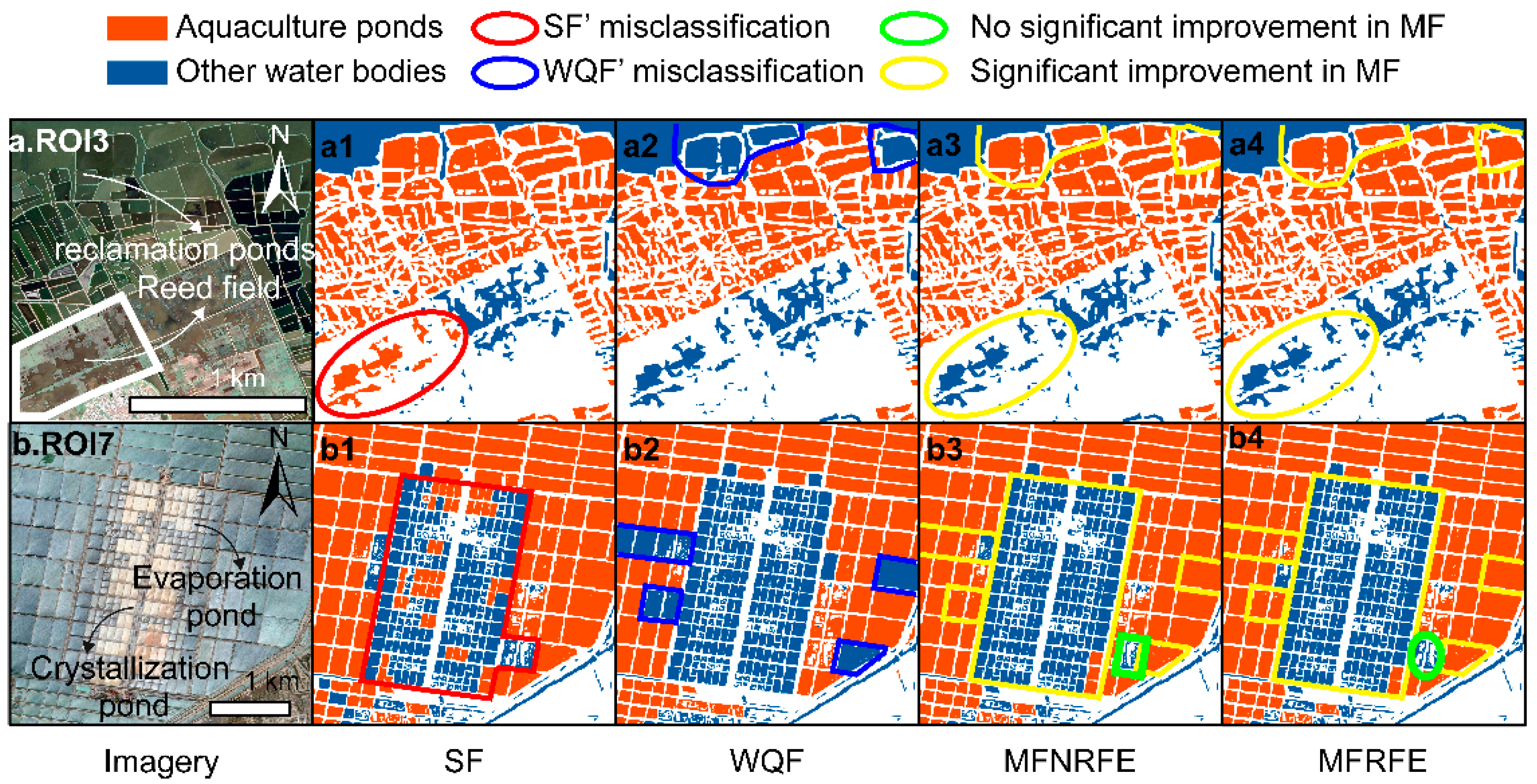
Figure 6.
The performance of the four test feature combinations on sites 1, 2, 4, 5, 6, and 8; (a1–a4) represents the SF, WQF, MFNRFE, and MFRFE classification results, same for (b1–f4).
Figure 6.
The performance of the four test feature combinations on sites 1, 2, 4, 5, 6, and 8; (a1–a4) represents the SF, WQF, MFNRFE, and MFRFE classification results, same for (b1–f4).

Figure 7.
Histogram of cumulative area of aquaculture pond probability within a 50 km buffer zone in 12 coastal provinces in China from 2015 to 2020.
Figure 7.
Histogram of cumulative area of aquaculture pond probability within a 50 km buffer zone in 12 coastal provinces in China from 2015 to 2020.

Figure 8.
The comparison of the different extraction results of various coastal provinces in China shows that our results are in good agreement with other studies [18,27].

Figure 9.
Probability maps of aquaculture ponds at different MFs based on 2019 Sentienl-2 MSI images. (a) indicates the probability map of aquaculture ponds in the Pearl River Delta; (a1,a2) refer to the detailed mapping of the two positions 1 and 2 in (a). (b) indicates the probability map of aquaculture ponds in Bohai Bay. (b1,b2) refer to the detailed mapping of the two positions 1 and 2 in (b). (c) indicates the probability map of aquaculture ponds in the Yangtze River Delta. (c1–c4) refer to the detailed mapping of the four positions of 1, 2, 3, and 4 in (c).


Table 1.
List of acronyms used in the paper.
| Acronym | Meaning |
|---|---|
| OBIA | Object-based image analysis |
| GEE | Google Earth Engine |
| ROI 1-8 | Regions of interest |
| MSI | Sentinel-2 Multispectral Instrument |
| NDWI | Normalized Water Index |
| MNDWI | Modified NDWI |
| SF | shape features |
| WQF | water quality parameter feature combination |
| MFRFE | mixed feature recursive feature elimination |
| MFNRFE | mixed feature non-recursive feature elimination |
Table 2.
Classification characteristics of each site and the difficulties in extraction.
| Index | Shape | Area (km2) | Difficulty | |
|---|---|---|---|---|
| ROI1 | irregular | 0.01–1.16 | Diversity between pond categories | Figure 2(a1) |
| ROI2 | irregular | ~0.005 | Mixed pixels blur the pond boundary | Figure 2(b1) |
| ROI3 | irregular | 0.005–0.08 | Reed field confused with pond | Figure 2(c1) |
| ROI4 | irregular | ~0.02 | Mixed pixels blur the pond boundary | Figure 2(d1) |
| ROI5 | regular | ~0.02 | Mixed pixels blur the pond boundary | Figure 2(e1) |
| ROI6 | regular | ~0.01 | Mixed pixels blur the pond boundary | Figure 2(f1) |
| ROI7 | regular | 0.06–0.15 | Saltworks confused with pond | Figure 2(g1) |
| ROI8 | irregular | 0.01–1.55 | Combining ROI4 and ROI7 | Figure 2(h1) |
Table 3.
The band and spatial resolution information of the Sentinel-2 MSI (* represents the bands used in this study).
Table 3.
The band and spatial resolution information of the Sentinel-2 MSI (* represents the bands used in this study).
| Name | Pixel Size | Central Wavelength (nm) | Bandwidth (nm) | Description |
|---|---|---|---|---|
| B1 | 60 m | 443 | 20 | Aerosols |
| B2 * | 10 m | 490 | 65 | Blue |
| B3 * | 10 m | 560 | 35 | Green |
| B4 * | 10 m | 665 | 30 | Red |
| B5 * | 20 m | 705 | 15 | Red Edge 1 |
| B6 * | 20 m | 740 | 15 | Red Edge 2 |
| B7 | 20 m | 783 | 20 | Red Edge 3 |
| B8 * | 10 m | 842 | 115 | NIR |
| B8A | 20 m | 865 | 20 | Red Edge 4 |
| B9 | 60 m | 945 | 20 | Water vapor |
| B10 | 60 m | 1375 | 30 | Cirrus |
| B11 | 20 m | 1610 | 90 | SWIR 1 |
| B12 | 20 m | 2190 | 180 | SWIR 2 |
Table 4.
Shape and water quality parameters.
| Parameters | Equation | |
|---|---|---|
| Area | ||
| Aspect Ratio | [41] | |
| Compactness C | [40] | |
| LSI | [42] | |
| Perimeter | ||
| Surface Algal Bloom Index (SABI) | [49] | |
| Phycocyanin(2BDA) | [44] | |
| Chlorophyll (NDCI) | [45] | |
| Chlorophyll (MCI) | * | [50] |
| Colored Dissolved Organic Matter (CDOM) | [48] |
* Cwl refers to the Center wavelength (nm).
Table 5.
The F1M, SD, and NBP of the four test feature combinations at eight test areas (bold numbers indicate optimal feature combination under different assessment metrics).
Table 5.
The F1M, SD, and NBP of the four test feature combinations at eight test areas (bold numbers indicate optimal feature combination under different assessment metrics).
| Median F1-Score | Standard Deviation (10−2) | Number of Best Performance (103) | ||||||||||
|---|---|---|---|---|---|---|---|---|---|---|---|---|
| SF | WQF | MFNRFE | MFRFE | SF | WQF | MFNRFE | MFRFE | SF | WQF | MFNRFE | MFRFE | |
| ROI1 | 0.96 | 0.96 | 0.96 | 0.96 | 2.17 | 1.94 | 2.08 | 2.07 | 2.38 | 4.73 | 4.29 | 3.85 |
| ROI2 | 0.87 | 0.91 | 0.93 | 0.93 | 2.43 | 2.20 | 1.98 | 1.94 | 0.05 | 2.10 | 4.46 | 5.45 |
| ROI3 | 0.91 | 0.96 | 0.95 | 0.96 | 2.49 | 1.70 | 1.72 | 1.65 | 0.03 | 4.23 | 2.36 | 5.13 |
| ROI4 | 0.93 | 0.95 | 0.95 | 0.95 | 2.52 | 2.20 | 2.15 | 2.15 | 1.26 | 4.09 | 4.30 | 6.13 |
| ROI5 | 0.95 | 0.97 | 0.97 | 0.97 | 2.69 | 2.11 | 2.14 | 2.16 | 2.63 | 4.96 | 5.20 | 5.87 |
| ROI6 | 0.95 | 0.97 | 0.97 | 0.97 | 2.39 | 2.10 | 1.94 | 1.92 | 0.67 | 4.57 | 5.34 | 5.46 |
| ROI7 | 0.86 | 0.86 | 0.91 | 0.91 | 3.13 | 2.99 | 2.73 | 2.61 | 0.35 | 0.67 | 4.22 | 6.05 |
| ROI8 | 0.89 | 0.88 | 0.89 | 0.90 | 4.50 | 4.22 | 4.11 | 4.02 | 3.31 | 1.74 | 3.11 | 4.29 |
| Average | 0.91 | 0.93 | 0.94 | 0.94 | 2.79 | 2.43 | 2.36 | 2.31 | 1.33 | 3.39 | 4.16 | 5.28 |
Publisher’s Note: MDPI stays neutral with regard to jurisdictional claims in published maps and institutional affiliations. |
© 2022 by the authors. Licensee MDPI, Basel, Switzerland. This article is an open access article distributed under the terms and conditions of the Creative Commons Attribution (CC BY) license (https://creativecommons.org/licenses/by/4.0/).
Share and Cite
MDPI and ACS Style
Hou, Y.; Zhao, G.; Chen, X.; Yu, X. Improving Satellite Retrieval of Coastal Aquaculture Pond by Adding Water Quality Parameters. Remote Sens. 2022, 14, 3306. https://doi.org/10.3390/rs14143306
AMA Style
Hou Y, Zhao G, Chen X, Yu X. Improving Satellite Retrieval of Coastal Aquaculture Pond by Adding Water Quality Parameters. Remote Sensing. 2022; 14(14):3306. https://doi.org/10.3390/rs14143306
Chicago/Turabian StyleHou, Yuxuan, Gang Zhao, Xiaohong Chen, and Xuan Yu. 2022. "Improving Satellite Retrieval of Coastal Aquaculture Pond by Adding Water Quality Parameters" Remote Sensing 14, no. 14: 3306. https://doi.org/10.3390/rs14143306
Note that from the first issue of 2016, this journal uses article numbers instead of page numbers. See further details here.