Article

Quantifying the Influences of Driving Factors on Land Surface Temperature during 2003–2018 in China Using Convergent Cross Mapping Method

1
Key Laboratory of Agricultural Remote Sensing, Ministry of Agriculture and Rural Affairs/Institute of Agricultural Resources and Regional Planning, Chinese Academy of Agricultural Sciences, Beijing 100081, China
2
ICube Laboratory, UMR 7357, CNRS-University of Strasbourg, 300 bd S’ebastien Brant, CS 10413, F-67412 Illkirch, France
3
Hebei International Joint Research Center for Remote Sensing of Agricultural Drought Monitoring, School of Land Science and Space Planning, Hebei GEO University, Shijiazhuang 050031, China
4
Chongqing Engineering Research Center for Remote Sensing Big Data Application, School of Geographical Sciences, Southwest University, No. 2 Tiansheng Road, Beibei District, Chongqing 400715, China
*
Author to whom correspondence should be addressed.
Remote Sens. 2022, 14(14), 3280; https://doi.org/10.3390/rs14143280
Submission received: 2 June 2022 / Revised: 28 June 2022 / Accepted: 5 July 2022 / Published: 7 July 2022

Abstract

:
The relationship between land surface temperature (LST) and environmental factors is complex and nonlinear. To determine these relationships for China, this study analyzed the driving effects of air temperature, vegetation index, soil moisture, net surface radiation, precipitation, aerosols, evapotranspiration, and water vapor on LST based on remote-sensing and reanalysis data from 2003–2018, using a convergent cross-mapping method. During the study period, air temperature and net surface radiation were the dominant drivers of LST with a cross-mapping skill above 0.9. Vegetation index and evapotranspiration were the secondary drivers of LST with a cross-mapping skill that was higher than 0.5. Except for air temperature and net surface radiation, the direction and strength of the effects of the driving factors on LST were related to the climate type. The effects of air temperature and net radiation on LST diminished from north to south, indicating that LST was more sensitive to air temperature and net radiation in energy-limited regions. However, the effects of vegetation index and evapotranspiration on LST varied significantly across climate zones; that is, positive effects were mostly in non-monsoonal zones and negative effects were primarily in monsoonal zones. Our results quantified the driving role of environmental factors on LST and provided a comprehensive understanding of LST dynamics.

1. Introduction

In a complex climate system, anomalies in key variables often lead to chain effects, disrupt related variables, and even cause fluctuations in the entire system. Land surface temperature (LST), a central element in the climate system, plays a fundamental role in assessing land-atmosphere interactions and climate change. It is defined as a high priority parameter by the International Geosphere-Biosphere Programme and as an important climate variable by the Global Climate Observing System (GCOS) of the World Meteorological Organization [1]. LST anomalies have a significant impact on energy cycles, ecological balance, and even human life. Unfortunately, the drivers that cause changes in LST are not accurately determined. Therefore, detecting the causal relationship between drivers and LST is crucial for analyzing both temperature anomalies and climate change.
Over the past few decades, significant results have been obtained for LST and its drivers, such as the relationship between surface cover type, NDVI (Normalized Difference Vegetation Index), elevation, soil moisture, evapotranspiration, and surface radiation with LST [2,3,4,5,6]. Generally, studies have focused on the urban heat island effect, heat wave phenomenon, or the effect of vegetation changes on LST [7,8,9,10]. There are limited studies analyzing the relationship between LST and environmental factors from causality perspective, especially the analysis of multiple environmental factors and LST. Several non-causal methods have been frequently used to analyze the relationship between environmental factors and LST in previous studies, including the correlation coefficient method [11], linear regression [12], stepwise regression [13,14], and geographically weighted regression [15,16]. In addition, most studies have statistically analyzed the correlations between LST and environmental factors on a time series, assuming that the environmental factors with significant correlations are the drivers of LST. However, they have ignored the basic principle that correlations are not causal. Therefore, when studying the interaction between LST and environmental factors, it is important to determine whether there is a causal relationship between the two.
In recent years, there has been a proliferation of approaches to causality analysis, which can be classified into qualitative process models and data-driven models. Qualitative process models require sufficient theory and experience to analyze the causality of things; however, obtaining accurate and sufficient process knowledge is difficult and time-consuming. By contrast, data-driven approaches can provide multiple ways to find causal relationships based on large amounts of historical data. Data-driven methods have been widely applied to identify the causal relationships between variables [17,18,19,20,21,22,23,24,25]. The Granger causality (GC) test proposed by Granger [26] is considered to be one of the earliest data-driven causality detection methods. The GC test assumes that a causal relationship exists between two variables if the prediction of one variable can be significantly improved by combining the information from another variable. However, GC tests require variables to be independent of each other; therefore, they are not suitable for causality detection of nonlinear systems with coupled relationships. The geographic detector method proposed by Wang et al. [27] determines the role of influencing factors through the spatial divergence between the independent and dependent variables, which not only detects the influencing factors, but also provides the magnitude of the ability of the influencing factors to explain the spatial divergence of the dependent variables. However, it has certain requirements with respect to the data types of variables, especially the causality of continuous time series variables detection. Thus, the results can be anomalous.
The empirical dynamic modeling (EDM) causality detection method was proposed by Sugihara et al. [17]. This convergent cross mapping (CCM) method is a practical data-based causality detection method based on Takens’ theorem to identify causal relationships in complex nonlinear systems with coupling. According to historical studies, the CCM method can effectively identify causal relationships in non-separable nonlinear systems, while being an equation-free statistical method that is not controlled by models [28]. The CCM method can not only identify causal relationships between variables while effectively eliminating the effects of other factors, but can also eliminate pseudo-causal relationships caused by synchronization effects [29]. In addition, the high sensitivity of CCM methods to weakly coupled relationships in nonlinear systems can lead to their increasing interest and applications in various fields, such as fisheries, medicine, chemistry, climate change, environmental pollution, and ecology [30,31,32,33,34]. However, to the best of our knowledge, few studies have focused on the causal relationship between LST and environmental elements based on the CCM method.
The main objectives of this study were to (1) identify the causal relationships between LST and environmental factors based on the CCM method, (2) screen and eliminate pseudo-causal relationships caused by synchronous effects between LST and environmental factors, and (3) explore the direction and intensity of the driving factors on LST using scenario exploration. The remainder of this paper is organized as follows. Section 2 presents the data sources for the environmental factors. Section 3 introduces the methodology. Section 4 provides the results before the discussion in Section 5, and Section 6 concludes the study.

2. Materials and Methods

2.1. Satellite Products

The National Aerodynamics and Space Administration (NASA) Earth Observing System (EOS) Terra and Aqua satellites, equipped with MODIS (Moderate-Resolution Imaging Spectroradiometer) sensors, were launched in December 1999 and May 2002, respectively. In this study, several MODIS land products (V006) were used, including MODIS/Aqua Land Surface Temperature monthly L3 Global 0.05° SIN Grid (MYD11C3), MODIS/Aqua Normalized Difference Vegetation Index monthly L3 Global 0.05° CMG (MYD13C2), MODIS/Aqua Aerosol daily L2 10 km × 10 km Product (MYD04_L2), MODIS/Terra Evapotranspiration 8-day L4 Global 500 m SIN Grid (MYD16A2), and MODIS/Aqua Total Precipitable Water Vapor daily L2 5 km × 5 km Product (MYD05_L2).
The MYD11C3 product was obtained by synthesizing and averaging the values of the corresponding months in the MYD11C1 product. This product provided LST estimates for day (1:30 p.m.) and night (1:30 a.m.) overpass times [35,36,37,38]. This study limited the analysis to high-quality clear-sky pixels with an LST error ≤ 1 K using the MYD11C3 quality control (QC) layer. The MODIS Aqua overpass time roughly corresponded to the daily maximum LST, which occurred in the afternoon, and the daily minimum LST, which was after midnight. Therefore, the average of the two LSTs was used in this study.
As an indicator closely related to green biomass and leaf area indices at regional and global scales, NDVI has been widely recognized for studying the relationship between LST and vegetation [39]. The MYD13C2 product is analogous to MYD13C1 (Vegetation Indices 16-Day L3 Global 0.05° CMG) but is based on MYD13A3 (Vegetation Indices Monthly L3 Global 1 km SIN Grid) for a monthly temporal resolution. All other specs are maintained and the production features are retained. In this study, the MYD04_L2 and MYD05_L2 products were used to obtain AOD (Aerosol Optical Depth) and WV (Water vapour) factors. The selected bands of the two products were AOD_550_Dark_Target_Deep_Blue_Combined and water vapor infrared.
The MYD16A2 product was an 8-day composite dataset produced at a spatial resolution of 500 m. The algorithm used for the MYD16 product was based on the logic of the Penman-Monteith equation, which included inputs of daily meteorological reanalysis data along with Moderate Resolution Imaging Spectroradiometer (MODIS) remotely sensed data products, such as vegetation property dynamics, albedo, and land cover [40].

2.2. ESA-CCI Soil Moisture Data

The soil moisture dataset was provided by the European Space Agency (ESA) (http://esa-soilmoisture-cci.org (accessed on 1 November 2021)). ESA released the global soil moisture product, which included active microwave products, passive microwave products, and combined active-passive microwave products [41]. In this study, the combined active-passive microwave product was analyzed from 2003 to 2018. The dataset had a spatial resolution of 0.25° × 0.25° [42]. Moreover, its applicability in China was demonstrated by An et al. (2016) [43].

2.3. ERA5-Land and CRU Data

ERA5-Land is a reanalysis dataset that provides a consistent view of the evolution of land variables over several decades at an enhanced resolution compared with ERA5. ERA5-Land was produced by replaying the land component of the European Center for Medium-Range Weather Forecast (ECMWF) ERA5 climate reanalysis [44]. Three products were used in this study, including air temperature at 2 m above the ground, surface net solar radiation, and surface net thermal radiation, with a spatial resolution of 0.1° × 0.1°. The surface net solar radiation and surface net thermal radiation data were used to calculate the surface net radiation.
Monthly precipitation data from the latest version of the Climatic Research Unit Version 4.04 (CRU TS4.04) for the period 2003–2018 were used in this study. The CRU dataset was developed by the University of the East Anglia Climatic Research Unit. The CRU dataset was found to have a better temporally continuous availability than traditional weather station observations [45].
All data from 2003 to 2018 were spatially and temporally scaled at a uniform resolution of 0.05° and monthly time steps, respectively. Spatial resampling to a 0.05° resolution was performed by applying bilinear interpolation. Daily and 8-day composite data were averaged to obtain the monthly values. Data with zero values are treated as invalid pixels. A summary of these data is presented in Table 1.

3. Method

To analyze the causality between LST and its related environmental factors, five main procedures for causality detection were summarized as follows: (1) The CCM method was used to identify the causality between LST and environmental factors. (2) The seasonal surrogate test (SST) was used to remove pseudo-causality between the LST and environmental factors caused by the seasonal synchronization effect. (3) Multivariate EDM helped examine whether environmental factors had a stronger causal effect on LST. (4) The ECCM (Extend Convergence Cross Mapping) method was used to further identify pseudo-causality due to generalized synchronization and Moran effects. (5) Multivariate scenario exploration was employed to determine the direction and strength of the real driver on LST. Details of each procedure are described in the following sections. A flowchart of causality detection between the LST and environmental factors is shown in Figure 1.

3.1. CCM

The CCM provides a way to identify the causal relationship between two variables in a complex nonlinear system. The fundamental principle of the CCM method is as follows.
If variable x in a system acts on variable y, the historical information of x is recorded by y. The time series of y can be used to recover the historical information of x; that is, the historical values of y can be used to map the time series of x. Details can be found in the three animations provided by Sugihara et al. [17] (http://science.sciencemag.org/content/suppl/2012/09/19/science.1227079.DC1 (accessed on 1 November 2021)). For the CCM analysis, the simplex projection was used to predict x with the historical information of y [46]. Cross-mapping skill (ρccm) was defined as the Pearson correlation coefficient ρ between the predicted and actual values of x. If the value of ρccm increased with the length of the time series and convergence was achieved, the causal effect of x on y could be determined. The Mann-Kendall monotonicity detection method (M-K test) was used to determine the convergence of ρccm [47,48]. The validity of the CCM detection results is determined by the convergence of ρccm, whereby the CCM method requires the time series length of the data to be greater than 30 [17]. To further improve the accuracy of the results in this study, we only detect the pixels with time series length greater than 90.
To explore the driving factors of LST, eight environmental factors including air temperature (TA), normalized difference vegetation index (NDVI), soil moisture (SM), net surface radiation (RN), precipitation (PRE), aerosol optical depth (AOD), evapotranspiration (ET), and water vapor (WV) were selected as potential driving variables. In this study, the CCM method was used to analyze whether the aforementioned eight environmental factors affected the response variable LST.

3.2. SST

A similar seasonal cycle between LST and an environmental factor may result in a high value of ρccm, even if there is no causal relationship. This phenomenon is described as the seasonal synchronization effect [17,29]. In this case, the CCM method could not fully distinguish real causality or spurious correlation [49]. A null test with a surrogate time series was considered as an effective method to address this problem [20].
The time series of an environmental factor with seasonal cycle changes {Z} was decomposed into seasonal cycle series {Zs} and short-term fluctuation series {∆d}. {∆d} was randomly shuffled to obtain a new fluctuation series {∆d*}. Then, {∆d*} was added to the seasonal cycle series {Zs} to obtain the surrogate time series of the environmental factor, that is, {Z*} = {Zs} + {∆d*}. It has been established that {Z*} has the same seasonal cycle series as {Z} but a different fluctuation series. If {Z} is indeed the driver of LST, LST will be sensitive not only to the seasonal cycle series {Zs}, but also to the fluctuation series {∆d}. Therefore, LST should be better at predicting the actual series {Z} than the surrogate series {Z*}. The shuffling procedure was repeated 500 times to produce a set of surrogate series of environmental factors. The value of ρccm between the LST and each surrogate series was calculated. The environmental factor was retained if the value of ρccm between the LST and the actual series of environmental factors was significantly higher than that between the LST and the 500 surrogate series. Otherwise, the environmental factor was considered to have no causal relationship with LST and was rejected. Finally, a non-parametric one-sample Wilcoxon test was chosen to estimate whether the actual series of environmental factors had a stronger effect on LST than the surrogate series at a significant level (p < 0.05).

3.3. Multivariate EDM

For causality detection among random variables, the CCM method may not be able to accurately identify the driving effect of an environmental factor on LST, due to data limitations, such as time series length and breakpoints in the time series [29]. In this study, multivariate EDM was used to determine whether an environmental factor had a significant driving effect on LST by comparing the improvement in EDM forecasting skills [50]. In other words, if an environmental factor had a driving effect on LST, it would significantly improve the forecasting skill of the model by adding environmental factors into the multivariate EDM model.
In this study, a multivariate EDM model composed of the time series of an environmental factor and the lagged time series of LST was used to forecast the LST. Forecasting skill (ρ) is the correlation coefficient between the time series of the forecasted and the original LST. Forecast improvement is the difference between the forecasting skill of the model with the environmental factor (ρwith_factor) and that without the environmental factor (ρwithout_factor), that is, forecast improvement Δρ = ρwith_factor − ρwithout_factor. A non-parametric one-sample Wilcoxon test was used to test the significance (p < 0.05) of the forecasting improvement of the multivariate EDM model.

3.4. ECCM

In a complex system, the accuracy of causality detection is affected by the generalized synchronization and the Moran effects [29], which cannot be removed by the SST and multivariate EDM methods. Ye et al. (2015) addressed the above problems by considering different time lags. In an actual causal relationship, the driving variable x can only act on the present or future values of the response variable y and not on the past values of y. Therefore, in the cross-mapping process, the response variable y can only predict the present or past values of the driving variable x, but not the future values of x. Accordingly, when using the CCM method to detect causality between variables x and y, if there is a time lag in the driving effect, the time lag must be non-positive. Based on this concept, Ye et al. [29] proposed an extension of the CCM method (ECCM). First, the set of lagged time series of variable x was established; ρccm between each lagged time series and variable y was calculated separately, and the time lag corresponding to the optimal ρccm was selected. If time lag ≤ 0, there was a driving effect of variable x on y, and the driving effect has a time lag of lag length. If time lag > 0, there is no driving effect of x on y. In this study, we performed ECCM detection for all environmental factors and LST.

3.5. Multivariate Scenario Exploration

After removing the pseudo-causal relationship between the environmental factors and LST, a scenario analysis was conducted to further explore the direction and strength of the driving effect of the true driver on LST. Multivariate scenario analysis based on EDM is a method for empirically assessing the effect of small changes in the driver on LST, which can effectively assess the response of LST to fluctuations in the driver [20]. The specific steps of multivariate scenario analysis are detailed below. Taking air temperature (TA) as an example, we predicted the effect of small changes in TA on LST for a corresponding lag length. The multivariate EDM model in this study included the lagged coordinates of the LST and the time series of TA:
L S T ( t + l a g ) f ( L S T ( t ) , L S T ( t 1 ) , , L S T ( t ( E 2 ) ) , T A ( t ) )
This equation was obtained with S-maps, where E is the optimal number of coordinates for the model to make predictions. For each historical time point t, this study predicted the LST with a small increase (+ΔTA/2) and a small decrease (−ΔTA/2) in the historically measured driver TA(t). To compare the strength of the effect of TA on LST in different regions, ΔTA was used, which corresponded to ~5% of the standard deviation of TA across China.
L S T + ( t + l a g ) f ( L S T ( t ) , L S T ( t 1 ) , , L S T ( t ( E 2 ) ) , T A ( t ) + Δ T A / 2 )
L S T ( t + l a g ) f ( L S T ( t ) , L S T ( t 1 ) , , L S T ( t ( E 2 ) ) , T A ( t ) Δ T A / 2 )
Δ L S T ( t ) / Δ T A = ( L S T + ( t + l a g ) L S T ( t + l a g ) ) / Δ T A
The value of Δ L S T ( t ) / Δ T A indicates the magnitude of the effect of TA on LST and the sign indicates the direction of the effect.

4. Results

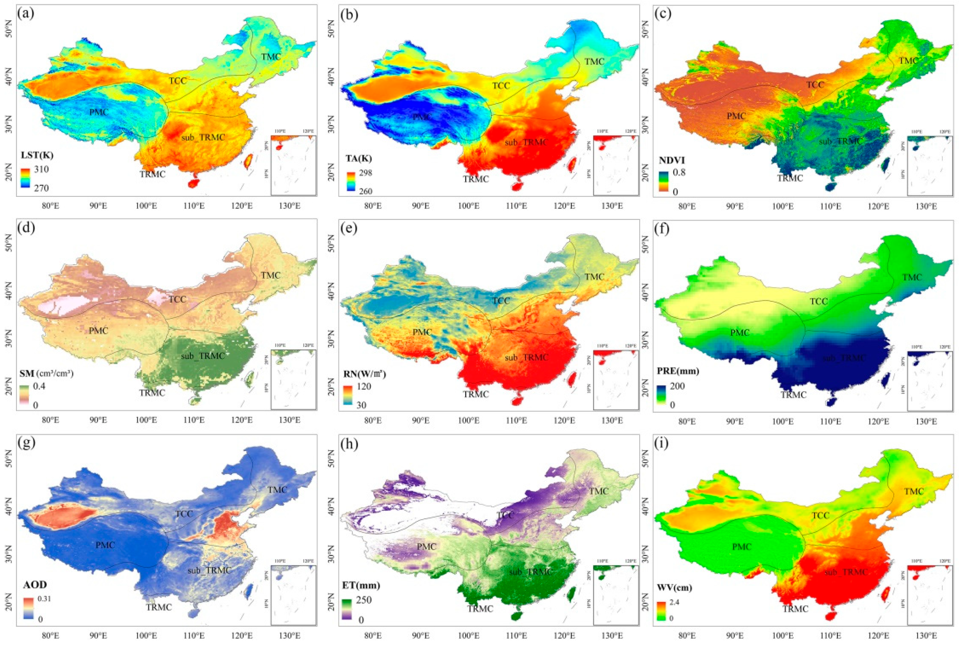
4.1. Spatial Pattern of LST and Environmental Factors

Figure 2 displays the spatial distribution of the multi-year mean LST and eight environmental factors in China from 2003 to 2018. The spatial distribution of LST showed an obvious latitudinal characteristic; that is, it decreased with increasing latitude. In addition, it showed different patterns influenced by altitude. For example, the Qinghai-Tibet Plateau in the southwest, which is the highest-altitude region in China, showed low temperatures at lower latitudes. The spatial distribution of TA was basically the same as that of LST, but it was approximately 5–9 K lower in magnitude than LST. NDVI and SM showed a distribution pattern that increased gradually from northwest to southeast, whereas RN and PRE showed a gradual increase from south to north. AOD was significantly higher in the northwest desert region and in the eastern region with higher population density; however, it was lower in all other regions. The magnitude of ET was strongly related to vegetation type; therefore, it was similar to NDVI in terms of spatial distribution. However, there was a large amount of missing data (blank areas in Figure 2h) in the northwest because the region was covered with deserts, especially Gobi. WV decreased from the coast to the inland and was at its lowest in the Qinghai-Tibet Plateau region, due to its leading altitude and topography.

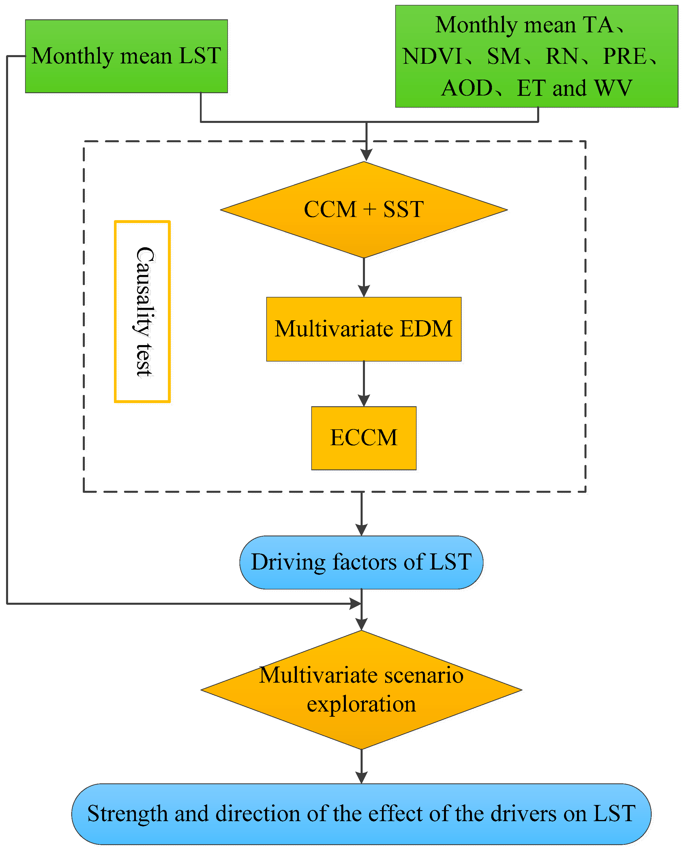
4.2. Causality Detection Process between LST and Environmental Factors

To clearly express the process of causality detection between LST and environmental factors, a pixel with grassland land cover type from the PMC region was selected as an example for a detailed demonstration. To ensure more stable results, each pair of cross-mapping processes was repeated 100 times [19], and the average of the 100 results was used as the final result. Figure 3 shows the detection results between LST and each environmental factor, with the horizontal axis being the length of the time series and the vertical axis being the ρccm between LST and environmental factors.
As shown in Figure 3, the ρccm curves between LST and each environmental factor exhibited different trends with an increase in the length of the time series. Among them, ρccm between RN and LST, TA and LST, and NDVI and LST increased rapidly with increasing time series length, and converged to 0.99, 0.97, and 0.91, respectively. This indicated strong potential causal relationships between RN and LST, TA and LST, and NDVI and LST. Although the ρccm between ET and LST, PRE and LST, and WV and LST showed monotonically increasing and converging characteristics, the corresponding ρccm values at convergence were relatively small, that is, 0.48, 0.42, and 0.38, respectively. This revealed that the strength of the potential causal relationships between them and LST was relatively low. The ρccm values between SM and LST, and AOD and LST decreased with increasing time series, indicating that there was no causal relationship between them and LST. The monotonic convergence of ρccm between environmental factors and LST was tested using the Mann-Kendall monotonicity test [51]. The results showed that ρccm between LST and all variables, except SM and AOD, showed significant monotonic increases (p < 0.05) and convergence characteristics.
A pseudo-causal relationship between LST and environmental factors can be caused by seasonal synchronization effects. For this reason, SST tests were conducted for LST and environmental factors, except SM and AOD. The test results are shown in Figure 4, where the red circles indicate the ρccm between LST and environmental factors, and the boxes indicate the ρccm between LST and the 500 seasonal surrogate series of environmental factors. The red solid circles demonstrate that the ρccm between the LST and the environmental factor is significantly larger than the ρccm between the seasonal surrogate series and the environmental factor; that is, the causal relationship between the LST and the environmental factor is not influenced by seasonal synchronization effects. The red hollow circles indicate a pseudo-causal relationship between the LST and environmental factors caused by seasonal synchronization effects. The SST results showed a pseudo-causal relationship between PRE and LST within this pixel.
In the case of random variables, CCM and SST causality tests can be misleading because of data limitations. In this study, variables that passed the SST test were introduced into the multivariate EDM model, and this pseudo-causality was removed by examining the extent to which the variables improved the forecasting skill of the multivariate EDM model. Figure 5 shows the improvement in the forecast skill of the multivariate EDM model for LST with the addition of each environmental factor separately. The blue bars indicate the forecast skill of the multivariate EDM model for LST without the addition of environmental factors, whereas the red bars indicate the degree of improvement in the model forecast skill with the addition of environmental factors. Overall, the forecast skill of the multivariate EDM model was significantly improved by the addition of TA, NDVI, RN, ET, and WV to this pixel (p < 0.05), indicating that there was a causal relationship between the above five environmental factors and LST. RN (0.22) had the greatest improvement in the forecast skill of the model, followed by NDVI (0.17), WV (0.11), TA (0.08), and ET (0.07).
Detection of the generalized synchrony effect and the Moran effect between variables is still an indispensable step in causality detection; therefore, this study further performed the ECCM test between the LST and the five environmental factors mentioned above. The spurious driving effect of the environmental factors on LST was removed by determining the time lag length of the effect of environmental factors on LST. Figure 6 shows the results of the ECCM between the LST and each environmental factor. The time lags set in this study were four months before and after LST, and the optimal ρccm between the five environmental factors and LST were all negative. This demonstrated that the environmental factors had a real driving effect on LST and were not affected by the generalized synchronization effect or the Moran effect. The lag lengths also represented the lags in the driving effect of environmental factors on LST.
In summary, after performing CCM causality tests between LST and environmental factors, and conducting pseudo-causality tests, such as SST, multivariate EDM, and ECCM tests, we identified TA, NDVI, RN, ET, and WV as drivers of LST change within this pixel.
Once the drivers of LST were identified, the direction and strength of the effects of the drivers on LST were analyzed using multivariate scenario analysis. Figure 7 shows the degree of response of the LST to small changes in the five drivers within this pixel, with the horizontal axis showing the drivers and the vertical axis indicating the degree of response of the LST. The results revealed that TA, NDVI, and RN had a positive driving effect on LST; that is, LST increased as the driving factor increased. Moreover, ET and WV had a negative driving effect on LST, that is, LST decreased as the driving factor increased. In addition, RN had the strongest effect on LST with a mean value of 0.58, followed by NDVI with a mean value of 0.13. TA had a relatively weak positive driving effect on LST with a mean value of 0.10. ET and WV had weak negative effects on LST with mean values of −0.04 and −0.02, respectively.

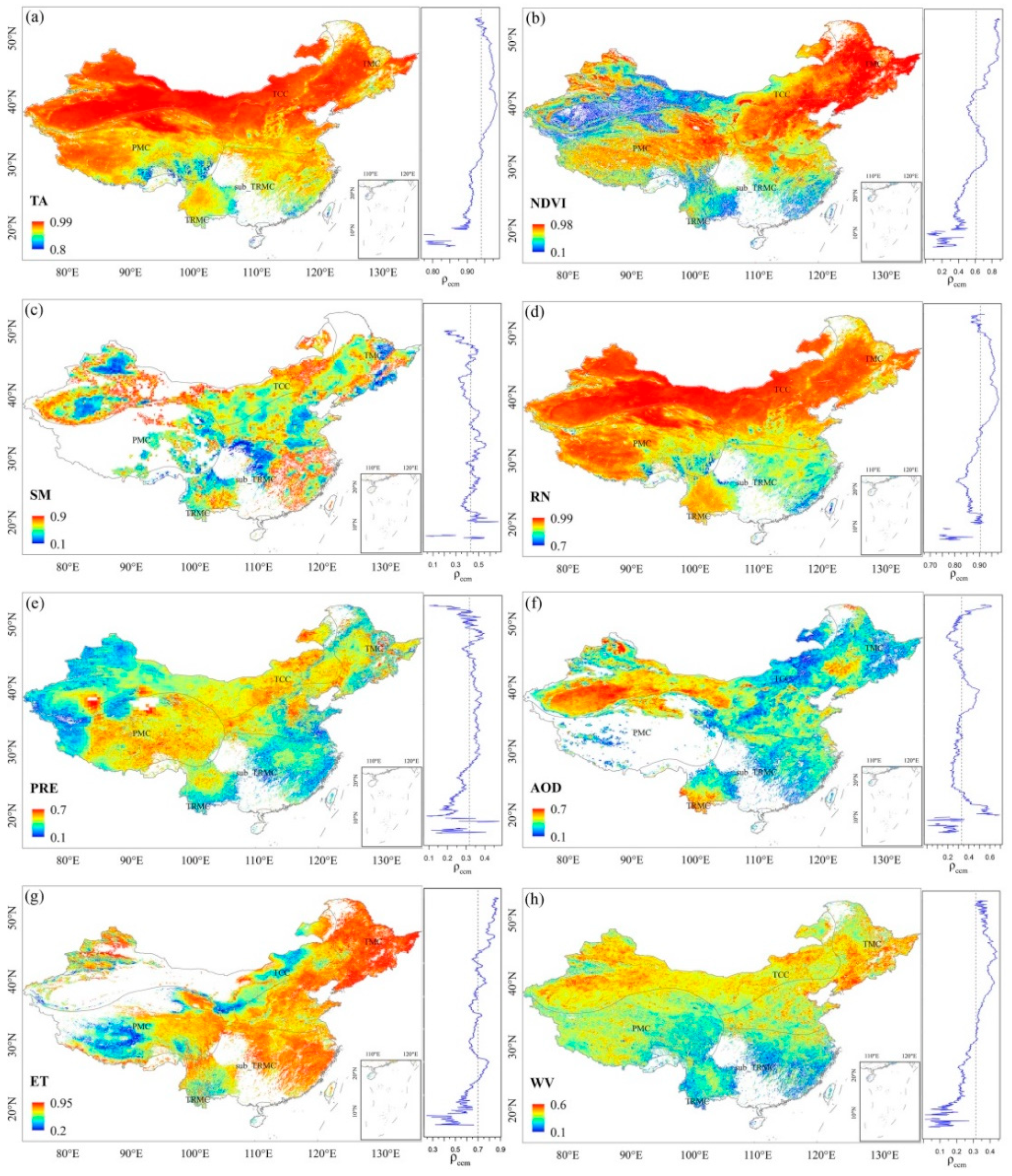
4.3. Result of CCM and SST Tests of China

Causality tests were conducted on a pixel-by-pixel basis to examine the causal relationships between LST and each environmental factor across China. The spatial distribution of ρccm between the LST and each environmental factor, as shown in Figure 8, was the result of the CCM and SST tests. The right-hand side of each panel corresponds to the latitudinal distribution of the mean value of ρccm. Overall, the ρccm of TA and RN were above 0.8 and 0.7, respectively, followed by NDVI and ET. However, the spatial variability between them was large, with variations ranging from 0.1 to 0.98 and 0.2 to 0.95, respectively. The ρccm of SM, PRE, AOD, and WV were relatively small.
From the perspective of latitudinal distribution, the ρccm of TA increased with increasing latitude and was less than the mean value of 0.94 south of 37°N, and greater than the mean value of 0.94 between 37°N and 53°N. It saw a decline north of 53°N. The ρccm of NDVI also increased with increasing latitude, but increased rapidly between 30°N and 35°N, and then decreased between 35°N and 40°N. This may be because the region between 30–35°N is the highest altitude Qinghai-Tibet Plateau region, while 35°–40°N falls within the largest desert in China. The ρccm of the SM varied less with latitude, fluctuating around a mean value of 0.43. The ρccm of RN had similar distribution characteristics to TA with respect to latitude, with a mean value of 0.91. The ρccm of the PRE was generally lower south of 32°N and north of 53°N, as compared to the other latitudinal zones. The ρccm of AOD was significantly higher than the mean between 38°N and 43°N. This is because the main surface cover type in this region was bare ground with little rain, high dust content in the air, and increased aerosol impact on LST. The ρccm of ET gradually increased from low to high latitudes, with a mean value of 0.70. The ρccm value of WV also increased with increasing latitude, but with a smaller mean value of 0.31.
Figure 9 presents the statistics of ρccm between LST and each environmental factor across climate zones. The results showed that the ρccm values of TA and RN were still relatively strong compared to other factors in the same climate zone. TA and RN had the strongest ρccm in TCC regions with mean values of 0.98 and 0.97, respectively, while they had the weakest ρccm in TRMC with mean values of 0.89 and 0.90, respectively. For NDVI and ET, the strongest mean values of ρccm were found in the TMC region, with mean values of 0.84 and 0.80, respectively. This may be due to the significant seasonal variation in vegetation in the TMC region, which strengthens the influence of NDVI on LST. In addition, the warmer and wetter monsoon climate enhanced the role of ET. However, the ρccm values of NDVI and ET were the weakest in the TRMC region, with mean values of 0.38 and 0.54, respectively. This suggested that the strength of the potential causal relationships between NDVI and LST as well as ET and LST were limited by hydrothermal conditions.

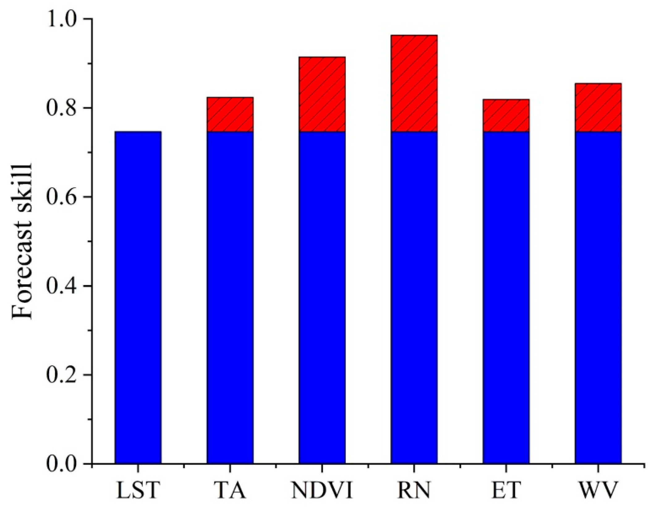
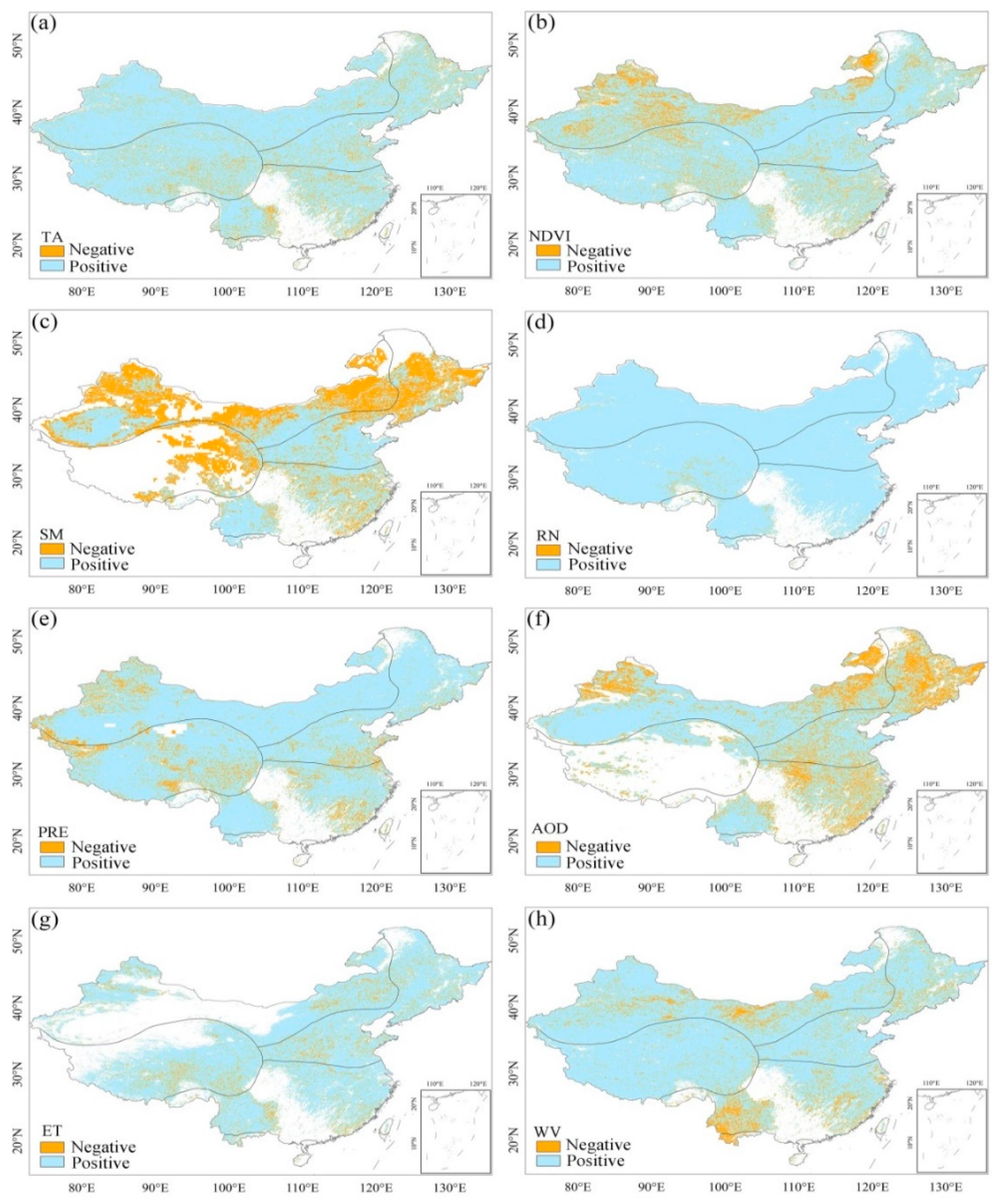
4.4. Pseudo-Causality Detection by Multivariate EDM

Figure 10 demonstrates the results of the multivariate EDM test between the environmental factors and LST after detection using CCM and SST. It can be seen that the results of multivariate EDM are presented in two categories: the forecast skill of the model with improvement (blue) and without improvement (yellow). For regions where the forecast skill of the multivariate EDM was not improved, causal relationship between the environmental factor and LST was considered to be pseudo-causal.
As can be seen from Figure 10, the forecast skill of the multivariate EDM with the addition of RN was significantly improved over the full domain, with only a sporadic area in the southern part of the Tibetan Plateau showing no improvement, accounting for less than 1%. Apart from RN, the forecast skill of the model after the addition of TA, PRE, ET, or WV also showed remarkable improvement; the regions that did not show betterment accounted for less than 10%. Pseudo-causality between NDVI and LST accounted for 13.29% of the total, mainly in the northern high latitudes where vegetation was sparse. Multivariate EDM detected a high proportion of pseudo-causal relationships between AOD and LST, at 25.26%, which was spread over most of the eastern region. SM had the highest pseudo-causal relationship with LST (43.33%), occupying almost all of northern China.

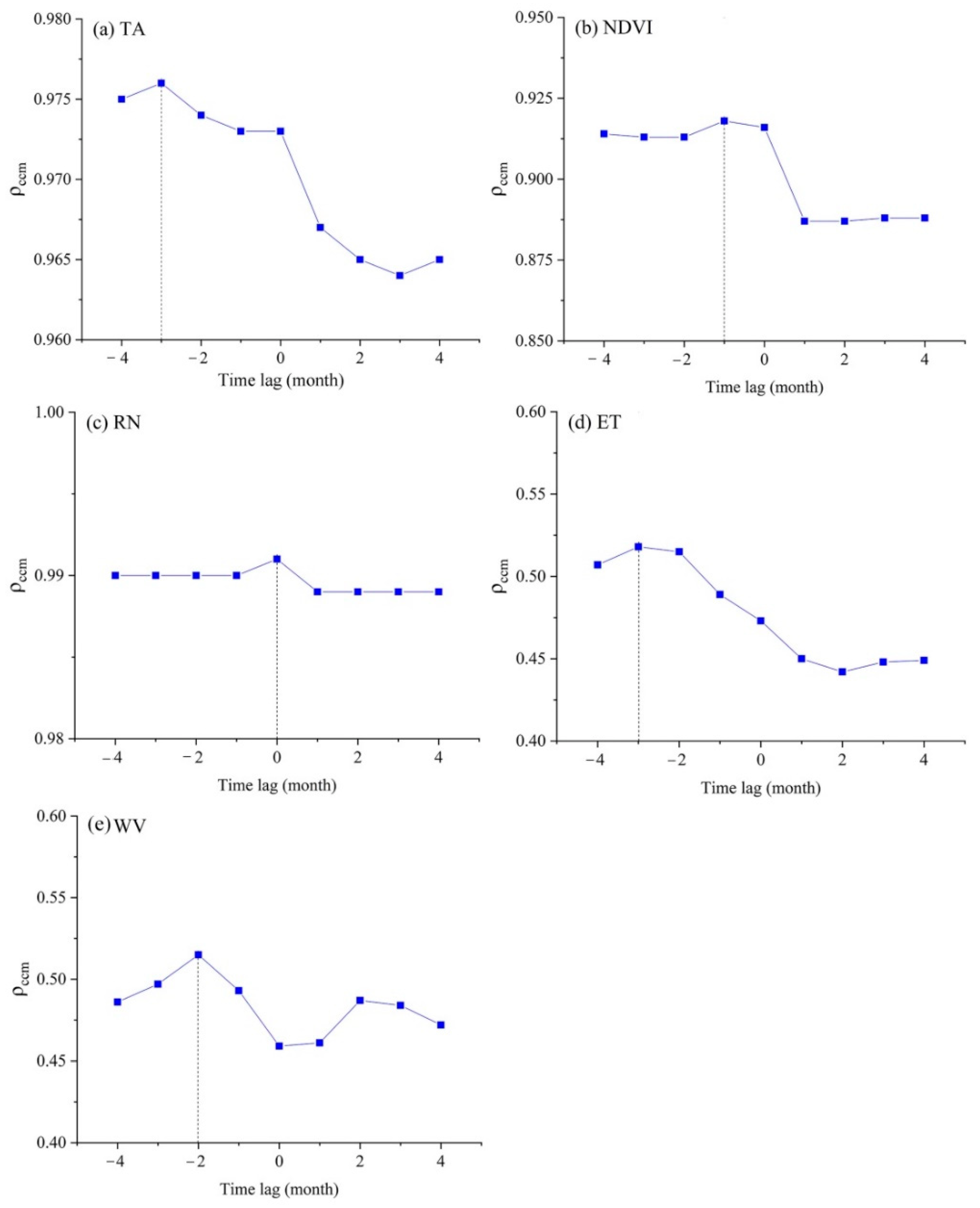
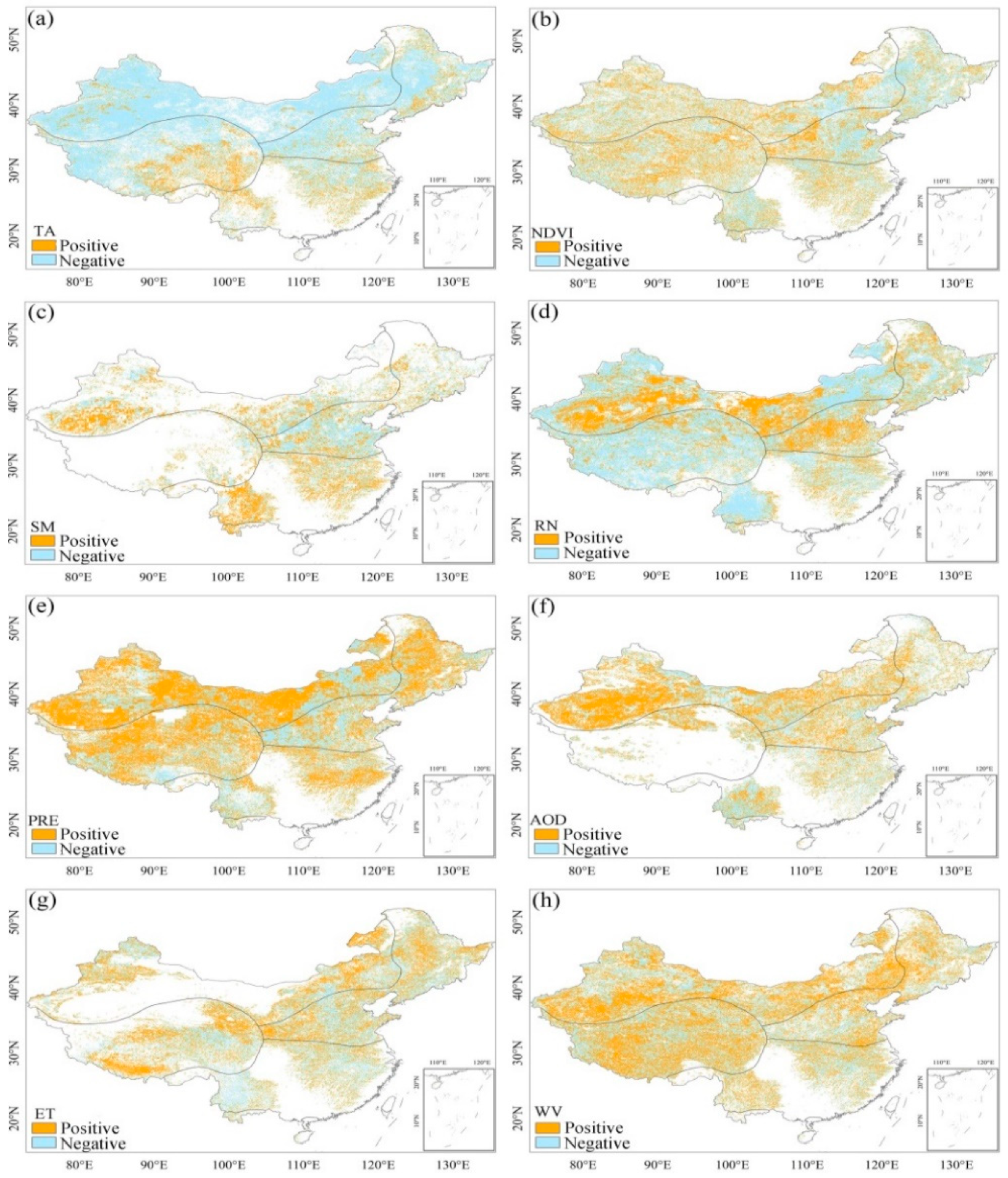
4.5. Pseudo-Causality Detection by ECCM

Figure 11 provides an overview of the results of ECCM detection between LST and environmental factors. Numerous positive time lags were detected for all factors due to generalized synchrony and Moran effects. Of these, the positive lag between TA and LST accounted for just 10.16%. Nearly 50% of these were distributed in the PMC region, probably because the PMC region was at an extremely high altitude and had the lowest air temperature in the study area. Therefore, its causal relationship with LST was not significant. The positive lag between RN and LST was 24.9%; approximately 20% of the positive lags were distributed in the TCC and TMC regions. With the exception of TA and RN, the positive lag between LST and other environmental factors was evenly distributed across different climatic zones, accounting for over 30%. In particular, two factors, AOD and SM, accounted for approximately 50% of the positive lags. Thus, the causality of PRE and AOD with LST was not only weak, but at least half of them were false. However, a positive time lag detected between environmental factors and LST only indicates that environmental factors have no driving effect on LST. They do not negate the absence of a driving effect of LST on environmental factors.
After pseudo-causal elimination with SST, multivariate EDM, and ECCM, the proportion of each environmental factor as a driver of the LST was determined. As shown in Figure 12, the highest percentage of driving factors among the environmental factors at the national scale was TA, accounting for 50.11%. ρccm had a mean value of 0.96. From different climate zones, the mean value of ρccm between TA and LST, as well as the percentage as a driving factor, showed a gradual decrease from north to south, indicating that LST was influenced by TA in its scope and intensity, both of which gradually weakened from north to south. The ρccm of TA within the TCC was the largest, with a mean value of 0.98, and the percentage of driving factor was 70%. The mean value of ρccm within the TRMC was the smallest (0.90), with 11.08% as the driving factor. In addition to TA, RN also had a relatively high share of 46.9%, with a mean ρccm of 0.92. The climatic zone with the largest ρccm of RN was TCC with a mean value of 0.96 and a driver share of 46.91%, while the climatic zone with the largest driver share was PMC (57.74%), with a mean ρccm of 0.92. The proportion of NDVI as a driver of LST at the national scale was 34.28%, with a mean ρccm of 0.65. TMC was the climate zone with the largest ρccm of NDVI, with a mean value of 0.84 and a percentage of drivers of 45.87%. ET as a driver of LST was relatively low at 25.4%, but ρccm was higher than NDVI with a mean value of 0.74. The climate zone with the highest proportion of ET as a driver of LST was TMC, with a proportion of 40.54% and a mean value of 0.81 for ρccm. The percentages of drivers in SM, AOD, PRE, and WV were 16.43%, 19.71%, 30.14%, and 30.36%, respectively, and with the mean ρccm of 0.48, 0.37, 0.36, and 0.34, respectively.

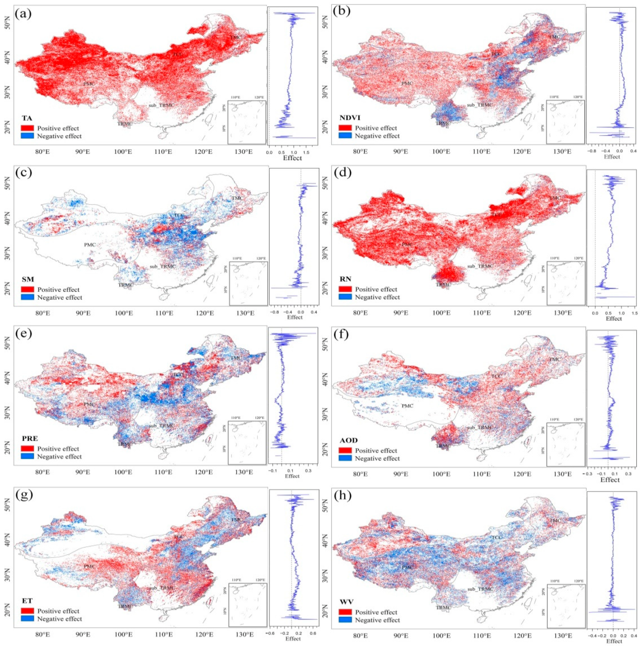
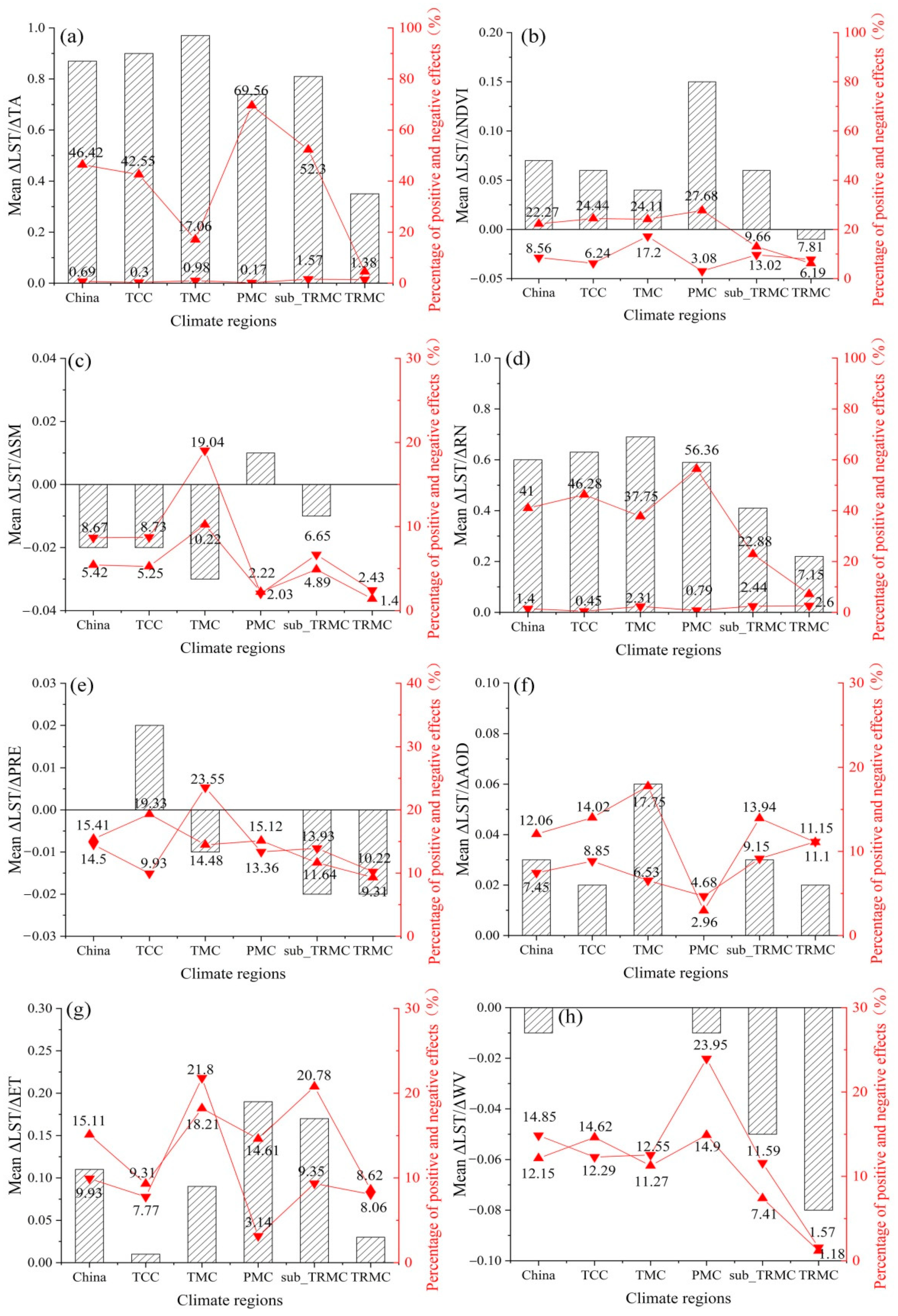
4.6. Effect of Driving Factors on LST

Having identified the drivers of LST over the study period, we analyzed the driving effect of the drivers. Figure 13 shows the spatial distribution of the results of the scenario analysis between each driver and LST. The red areas indicate a positive effect of the drivers on LST and the blue areas indicate a negative effect of the drivers on LST. The results revealed that there was a positive effect on LST at the national level, as shown in Figure 13a,d. A similar relationship between TA, RN, and LST was also reported in previous studies [52,53,54]. The positive effects of NDVI on LST were mostly found in the TCC and PMC regions (Figure 13b); however, both climate regions had restricted energy access. The negative effect of NDVI on LST was mostly observed in the TMC, sub_TRMC, and TRMC regions. This result reaffirmed the conclusion of Karnieli et al. [55] that the interaction between LST and NDVI is positive when energy is limited (high latitude or high altitude) and negative when energy is available [56]. In addition, the positive effect of ET on LST was mainly concentrated in the eastern part of the TCC region, most of the PMC region, and central part of the sub_TRMC region. Sun et al. [2] stated that the limits of TA and SM should be considered when analyzing the relationship between ET and LST. However, in this study, the interaction between ET and LST were related to land cover type. AOD had a predominantly positive effect on LST, whereas the regions that showed a negative effect were mainly located in the western part of the TCC region. Studies have shown that the impact of aerosols on climate depends not only on the quantity of aerosols but also on their optical properties. Aerosols affect LST by influencing the solar radiation reaching the surface. Scattering aerosols having a cooling effect as they reduce the energy received at the surface, whereas absorbing aerosols have a warming effect [55]. The large amount of dust aerosols produced in the Taklamakan Desert in northwest China increased the reflection of solar radiation from the surface, which may have been the main reason for the negative effect of AOD on LST. The positive effect of AOD on LST embodied in other regions was mainly due to the anthropogenic emissions of absorptive aerosols.
The latitudinal distribution shows the strength of the effect of each driver on LST and its variation with latitude. Overall, among the drivers, only TA and RN had a positive effect on LST. The intensity of the effect of both was greater, ranging between 0 and 1.5. The effect of NDVI on LST varied across latitudes, with a negative effect south of about 27°N and north of 53°N, and a positive effect between 27°N and 53°N. The intensity of the effect of NDVI on LST was mostly distributed between −0.4 and 0.4. Furthermore, ET had a significant positive effect on LST between 25°N and 38°N, reaching 0.2.
In different climatic regions, there were significant differences in the manner and intensity of the effect of the driver (Figure 14). At a national level, the positive effect of TA on LST was 46.42%, whereas the negative effect was only 0.69%. In terms of the mean value of the intensity of the effect TA on LST, it was maximum in the TMC region with a mean value of 0.97, in minimum in the TRMC region with a mean value of 0.35. This indicated that the effect of TA on LST was stronger at higher latitudes. The strength of RN’s effect on LST was second only to that of TA, with 41% positive and 1.4% negative effects. Regarding the mean value of the effect of RN on LST, the climatic region with the strongest effect of RN on LST was TMC with a mean value of 0.69; the weakest was TRMC with a mean value of 0.22. The positive effect of NDVI on LST was 22.27% and the negative effect was 8.56%. Of these, TCC, TMC, PMC, and sub_TRMC were positive and the highest within PMC, with a mean value of 0.15, while in TRMC, they were mainly negative with a mean value of −0.01. On LST, ET had a positive effect of 15.11% and a negative effect of 9.93%, with a greater intensity within PMC and sub_TRMC, with mean values of 0.19 and 0.17, respectively.

5. Discussion

5.1. Type of Causal Relationship between LST and Drivers

Recent studies have focused on the relationship between single variables and LST [10,11,14,57]. The identification of the driving role of multiple variables on LST and their dominant factors has rarely been studied. Furthermore, correlation analysis has been used in the methods used to study the relationship between LST and influencing factors, but it needs to be emphasized that correlation does not mean that a causal relationship exists. This study attempted to explore the dominant drivers of LST in terms of the causal relationship between multiple factors and LST. The CCM method, which is suitable for causality detection in nonlinear dynamical systems, was used to detect the causal relationship between each environmental factor and LST. The CCM test results were verified by SST, multivariate EDM, and ECCM, which showed that TA and RN were strong drivers of LST and had a much higher positive effect than other factors. Furthermore, NDVI and ET had relatively strong driving effects on LST, but they had both positive and negative effects in different regions.
In addition, the CCM method was used to identify whether there was a causal relationship between environmental factors and LST, but it could not determine whether the driving effect was unidirectional or bidirectional. To determine the interaction pattern between each driver and LST, this study used the CCM method to test the driving effect of LST on environmental factors and performed a pseudo-causality test. The interactions between LST and environmental factors were classified into three categories: environmental factors driving LST, LST driving environmental factors, and mutual drive.
Figure 15 show the spatial distribution of the pattern of causal interaction between LST and drivers and the share of each type, respectively. Total of the three causality types between RN and LST accounted for 79.38% of the country and 20.62% had no causality (Figure 15d). Among them, bidirectional causality accounted for 48.49% and was widely distributed, while the type of LST-driven RN accounted for 20.23% and was mainly distributed in the TCC and southern part of TMC, where RN was lower. Second to RN, the areas with causality between TA and LST accounted for 78.04% of the whole country land area, while 21.96% of the areas had no causality (Figure 15a). The type of causality was mainly bidirectional, accounting for 63.36% of the country, and was mainly distributed in the TCC, TMC, and PMC regions. The causality between NDVI and LST was 34.18%, 16.31%, and 16.34% for bidirectional, LST-driven NDVI, and NDVI-driven LST, respectively, and 33.18% had no causality (Figure 15b). PRE was the only variable among the selected environmental factors that was dominated by reverse causality, that is, LST-driven PRE type causality was dominant (31.32%), and mainly in the TCC and PMC areas, which was higher than the proportion of bidirectional causality at 24.79% (Figure 15e). In addition, the WV-driven LST causality type accounted for the largest proportion of the three causality types (25.21%). For SM and AOD, no causality has a large percentage of the country, with 68.81% and 57.9%, respectively.
Overall, the causality between LST and most drivers was predominantly bidirectional. On the other hand, few drivers, such as PRE and WV, were predominantly unidirectional.

5.2. Bidirectional Causality between LST and Drivers

For the bidirectional causality type, there is a need to understand the stronger direction. To this end, we calculated the difference (Δρccm) between ρccm in the positive direction (factor driving LST) and ρccm in the negative direction (LST driving factor).
Figure 16 shows the variation in Δρccm with latitude. Overall, all variables were dominated by negative differences, except for TA, which was dominated by positive differences. In the interaction between TA and LST, the intensity of the TA driving LST north of 37°N was higher than that of the LST driving TA. The difference between 37°N and 33°N was close to 0, indicating that the strength of the interaction between LST and TA was similar in this interval. Negative peaks occurred between 33°N and 27°N, and fluctuations in the difference were greater south of 27°N, which may be due to the small amount of data in this region. Generally, the difference in the strength of the causality between TA and LST in both directions was small, with Δρccm ranging from −0.05 to 0.1. The causality between NDVI and LST was dominated by the LST-driven NDVI direction throughout the country. The absolute value of Δρccm decreased gradually from south to north, indicating that LST drove NDVI more in the south. The difference in the strength of the two-way causality between RN and LST was also relatively small, dominated by LST-driven RN. There was a trend of stronger RN driving LST south of 25°N, with a negative peak between 25°N and 40°N. This decreased rapidly because of the extremely high altitude of the Tibetan Plateau in this region. The Δρccm between AOD and LST only showed a positive peak between 30°N and 35°N, with negative values in all other latitudinal zones, as the Beijing-Tianjin-Hebei region with high AOD values was distributed in this latitudinal zone. The strength of AOD driving LST was higher than that of LST driving AOD. The relationship between ET and LST was also dominated by LST driving ET, and Δρccm was relatively stable at all latitudes.
In summary, even though there was a bidirectional causal relationship between LST and each environmental factor, the dominant causal relationship was still in the direction of LST driving environmental factors.
In this study, CCM, SST, multivariate EDM, and ECCM were used to identify the true drivers of LST among environmental factors and to explore the interaction patterns between LST and drivers through multivariate scenario analysis. However, the complexity of surface eco-physical systems prevented a complete list of all variables associated with LST, and the diversity of data sources introduced inevitable errors in the experimental results. Therefore, a complete understanding of LST can be obtained from an integrated treatment of these constraints, which will provide a basis for future research.

6. Conclusions

This study explored the driving role of environmental factors (TA, NDVI, SM, RN, PRE, AOD, ET, and WV) and LST during 2003–2018 in China using the CCM, SST, multivariate EDM, and ECCM methods.
All environmental factors had driving effects on LST. However, after the removal of pseudo-causality and the comparison of the driving strength of each variable, TA and RN were concluded to be the dominant factors with high driving strengths, followed by NDVI and ET.
All drivers had positive as well as negative effects on LST, except for TA and RN, which only had positive effects on LST. The intensity of the effects of TA and RN on LST showed signs of weakening from high northern latitudes to low latitudes, indicating that LST was more strongly driven by TA and RN in regions with lower energy. The positive effects of NDVI and ET on LST were mainly distributed in the TCC and PMC zones, while the negative effects were mainly distributed in the TMC, sub_TRMC, and TRMC regions. This indicated that the direction of NDVI and ET effects on LST were limited by hydrothermal conditions. Overall, the positive effects were more significant at high latitudes and altitudes.
There are three types of causal relationships between LST and each environmental factor, that is, factor-driven LST, LST-driven factor, and bidirectional drive. However, the bidirectional causal relationship between LST and the driver is dominant. In addition, the categorization of causal relationships between LST and factors revealed that LST driving factors were dominant in quantity, except for SM and WV. In terms of driving strength, the driving effect of LST on factors was stronger than the driving strength of factors on LST, except for TA.
Our results quantify the driving effects of environmental factors on LST; however, future studies should explore the relationships between surface type, elevation, and slope orientation to fully understand the dynamics of LST.

Author Contributions

Writing—original draft preparation, Y.Y.; writing—review and editing, Y.Y., S.D. and J.L.; visualization, Y.Y.; formal analysis, Y.Y.; data curation, W.Y.; supervision, G.S. and Z.L.; funding acquisition, G.S. and S.D. All authors have read and agreed to the published version of the manuscript.

Funding

This work was supported partly by the National Science Foundation of China (Grant No. 42071326 and 41871275) and partly by the China Scholar Council (CSC) under Grant number 202003250102.

Data Availability Statement

Not applicable.

Acknowledgments

The authors would like to thank the MODIS Science teams at NASA for providing the satellite observation data. The MODIS products can be downloaded from the U.S. Geological Survey (USGS) Land Processes Distributed Active Archive Center (LP DAAC) (https://search.earthdata.nasa.gov (accessed on 1 November 2021)). We also acknowledge the European Space Agency Climate Change Initiative (ESA-CCI) (http://www.esa-soilmoisture-cci.org/ (accessed on 1 November 2021)), ERA5-Land (https://cds.climate.copernicus.eu/ (accessed on 15 October 2021)) and Climatic Research Unit (CRU) (https://crudata.uea.ac.uk/cru/data/ (accessed on 1 October 2021)), for providing research data.

Conflicts of Interest

The authors declare no conflict of interest.

References

  1. GCOS. GCOS 2016 Implementation Plan; World Meteorological Agency (WMO): Marrakesh, Morocco, 2016; Available online: https://library.wmo.int/doc_num.php?explnum_id=3417 (accessed on 10 November 2020).
  2. Sun, Z.; Wang, Q.; Batkhishig, O.; Ouyang, Z. Relationship between evapotranspiration and land surface temperature under energy- and water-limited conditions in dry and cold climates. Adv. Meteorol. 2016, 2016, 1–9. [Google Scholar] [CrossRef] [Green Version]
  3. Aguilar-Lome, J.; Espinoza-Villar, R.; Espinoza, J.; Rojas-Acuña, J.; Willems, B.; Leyva-Molina, W. Elevation-dependent warming of land surface temperatures in the Andes assessed using MODIS LST time series (2000–2017). Int. J. Appl. Earth Obs. Geoinf. 2019, 77, 119–128. [Google Scholar] [CrossRef]
  4. Abera, T.; Heiskanen, J.; Maeda, E.; Pellikka, P. Land surface temperature trend and its drivers in East Africa. J. Geophys. Res. Atmos. 2020, 125, 23. [Google Scholar] [CrossRef]
  5. Wu, H.; Li, Z.; Yu, X.; Zeng, Q.; Lin, J.; Chen, Y.; Ai, S.; Guo, P.; Lin, H. Empirical dynamic modeling reveals climatic drivers in dynamics of bacillary dysentery epidemics in China. Environ. Res. Lett. 2020, 15, 124054. [Google Scholar] [CrossRef]
  6. Yang, J.; Ren, J.; Sun, D.; Xiao, X.; Xia, J.; Jin, C.; Li, X. Understanding land surface temperature impact factors based on local climate zones. Sustain. Cities Soc. 2021, 69, 102818. [Google Scholar] [CrossRef]
  7. Guo, G.; Wu, Z.; Xiao, R.; Chen, Y.; Liu, X.; Zhang, X. Impacts of urban biophysical composition on land surface temperature in urban heat island clusters. Landsc. Urban Plan. 2015, 135, 1–10. [Google Scholar] [CrossRef]
  8. Luyssaert, S.; Jammet, M.; Stoy, P.; Estel, S.; Pongratz, J.; Ceschia, E.; Churkina, G.; Don, A.; Erb, K.; Ferlicoq, M.; et al. Land management and land-cover change have impacts of similar magnitude on surface temperature. Nat. Clim. Change 2014, 4, 389–393. [Google Scholar] [CrossRef] [Green Version]
  9. Peng, S.; Piao, S.; Zeng, Z.; Ciais, P.; Zhou, L.; Li, L.; Myneni, R.; Yin, Y.; Zeng, H. Afforestation in China cools local land surface temperature. Proc. Natl. Acad. Sci. USA 2014, 111, 2915–2919. [Google Scholar] [CrossRef] [Green Version]
  10. Deng, Y.; Wang, S.; Bai, X.; Tian, Y.; Wu, L.; Xiao, J.; Chen, F.; Qian, Q. Relationship among land surface temperature and LUCC, NDVI in typical karst area. Sci. Rep. 2018, 8, 641. [Google Scholar] [CrossRef]
  11. Yu, Y.; Duan, S.; Li, Z.; Chang, S.; Xing, Z.; Leng, P.; Gao, M. Interannual spatiotemporal variations of land surface temperature in China from 2003 to 2018. IEEE J. Sel. Top. Appl. Earth Obs. Remote Sens. 2021, 14, 1783–1795. [Google Scholar] [CrossRef]
  12. Zhou, D.; Xiao, J.; Frolking, S.; Liu, S.; Zhang, L.; Cui, Y.; Zhou, G. Croplands intensify regional and global warming according to satellite observations. Remote Sens. Environ. 2021, 264, 112585. [Google Scholar] [CrossRef]
  13. Wu, X.; Wang, L.; Yao, R.; Luo, M.; Li, X. Identifying the dominant driving factors of heat waves in the North China Plain. Atmos. Res. 2021, 252, 105458. [Google Scholar] [CrossRef]
  14. Peng, W.; Zhou, J.; Wen, L.; Xue, S.; Dong, L. Land surface temperature and its impact factors in Western Sichuan Plateau, China. Geocarto Int. 2016, 32, 919–934. [Google Scholar] [CrossRef]
  15. Zhao, H.; Ren, Z.; Tan, J. The spatial patterns of land surface temperature and its impact factors: Spatial non-stationarity and scale effects based on a Geographically-Weighted Regression Model. Sustainability 2018, 10, 2242. [Google Scholar] [CrossRef] [Green Version]
  16. Wang, W.; Samat, A.; Abuduwaili, J.; Ge, Y. Quantifying the influences of land surface parameters on LST variations based on GeoDetector model in Syr Darya Basin, Central Asia. J. Arid Environ. 2021, 186, 104415. [Google Scholar] [CrossRef]
  17. Sugihara, G.; May, R.; Ye, H.; Hsieh, C.; Deyle, E.; Fogarty, M.; Munch, S. Detecting causality in complex ecosystems. Science 2012, 338, 496–500. [Google Scholar] [CrossRef]
  18. Chen, Z.; Zhuang, Y.; Xie, X.; Chen, D.; Cheng, N.; Yang, L.; Li, R. Understanding long-term variations of meteorological influences on ground ozone concentrations in Beijing During 2006–2016. Environ. Pollut. 2019, 245, 29–37. [Google Scholar] [CrossRef]
  19. Clark, A.; Ye, H.; Isbell, F.; Deyle, E.; Cowles, J.; Tilman, G.; Sugihara, G. Spatial convergent cross mapping to detect causal relationships from short time series. Ecology 2015, 96, 1174–1181. [Google Scholar] [CrossRef]
  20. Deyle, E.; Maher, M.; Hernandez, R.; Basu, S.; Sugihara, G. Global environmental drivers of influenza. Proc. Natl. Acad. Sci. USA 2016, 113, 13081–13086. [Google Scholar] [CrossRef] [Green Version]
  21. Wang, Y.; Yang, J.; Chen, Y.; De Maeyer, P.; Li, Z.; Duan, W. Detecting the causal effect of soil moisture on precipitation using Convergent Cross Mapping. Sci. Rep. 2018, 8, 12171. [Google Scholar] [CrossRef]
  22. Wang, Y.; Hu, F.; Cao, Y.; Yuan, X.; Yang, C. Improved CCM for variable causality detection in complex systems. Control. Eng. Pract. 2019, 83, 67–82. [Google Scholar] [CrossRef]
  23. Chen, Z.; Chen, D.; Zhao, C.; Kwan, M.; Cai, J.; Zhuang, Y.; Zhao, B.; Wang, X.; Chen, B.; Yang, J.; et al. Influence of meteorological conditions on PM2.5 concentrations across China: A review of methodology and mechanism. Environ. Int. 2020, 139, 105558. [Google Scholar] [CrossRef] [PubMed]
  24. Chen, Z.; Li, R.; Chen, D.; Zhuang, Y.; Gao, B.; Yang, L.; Li, M. Understanding the causal influence of major meteorological factors on ground ozone concentrations across China. J. Clean. Prod. 2020, 242, 118498. [Google Scholar] [CrossRef]
  25. Barraquand, F.; Picoche, C.; Detto, M.; Hartig, F. Inferring species interactions using Granger causality and convergent cross mapping. Theor. Ecol. 2020, 14, 87–105. [Google Scholar] [CrossRef]
  26. Granger, C. Investigating Causal Relations by Econometric Models and Cross-spectral Methods. Econometrica 1969, 37, 424. [Google Scholar] [CrossRef]
  27. Wang, J.; Zhang, T.; Fu, B. A measure of spatial stratified heterogeneity. Ecol. Indic. 2016, 67, 250–256. [Google Scholar] [CrossRef]
  28. Liu, H.; Lei, M.; Zhang, N.; Du, G. The causal nexus between energy consumption, carbon emissions and economic growth: New evidence from China, India and G7 countries using convergent cross mapping. PLoS ONE 2019, 14, e0217319. [Google Scholar] [CrossRef]
  29. Ye, H.; Deyle, E.R.; Gilarranz, L.J.; Sugihara, G. Distinguishing time-delayed causal interactions using convergent cross mapping. Sci. Rep. 2015, 5, 14750. [Google Scholar] [CrossRef] [Green Version]
  30. Deyle, E.R.; Fogarty, M.; Hsieh, C.-H.; Kaufman, L.; MacCall, A.D.; Munch, S.B.; Perretti, C.T.; Ye, H.; Sugihara, G. Predicting climate effects on Pacific sardine. Proc. Natl. Acad. Sci. USA 2013, 110, 6430–6435. [Google Scholar] [CrossRef] [Green Version]
  31. Heskamp, L.; Abeelen, A.S.M.-V.D.; Lagro, J.; Claassen, J.A. Convergent cross mapping: A promising technique for cerebral autoregulation estimation. Int. J. Clin. Neurosci. Ment. Health 2014, 1, S20. [Google Scholar] [CrossRef] [Green Version]
  32. Luo, L.; Cheng, F.; Qiu, T.; Zhao, J. Refined convergent cross-mapping for disturbance propagation analysis of chemical processes. Comput. Chem. Eng. 2017, 106, 1–16. [Google Scholar] [CrossRef]
  33. Zhang, J.; Zhang, Y.; Qin, S.; Wu, B.; Wu, X.; Zhu, Y.; Shao, Y.; Gao, Y.; Jin, Q.; Lai, Z. Effects of seasonal variability of climatic factors on vegetation coverage across drylands in northern China. Land Degrad. Dev. 2018, 29, 1782–1791. [Google Scholar] [CrossRef]
  34. Wang, J.-Y.; Kuo, T.-C.; Hsieh, C.-H. Causal effects of population dynamics and environmental changes on spatial variability of marine fishes. Nat. Commun. 2020, 11, 2635. [Google Scholar] [CrossRef] [PubMed]
  35. Wan, Z.; Li, Z.-L. A physics-based algorithm for retrieving land-surface emissivity and temperature from EOS/MODIS data. IEEE Trans. Geosci. Remote. Sens. 1997, 35, 980–996. [Google Scholar] [CrossRef]
  36. Wan, Z.; Zhang, Y.; Zhang, Q.; Li, Z.L. Validation of the land-surface temperature products retrieved from Terra Moderate Resolution Imaging Spectroradiometer data. Remote Sens. Environ. 2002, 83, 163–180. [Google Scholar] [CrossRef]
  37. Wan, Z.; Li, Z. Radiance-based validation of the V5 MODIS land-surface temperature product. Int. J. Remote Sens. 2008, 29, 5373–5395. [Google Scholar] [CrossRef]
  38. Wan, Z.; Li, Z.-L. MODIS land surface temperature and emissivity. In Land Remote Sensing and Global Environmental Change; Springer: Berlin/Heidelberg, Germany, 2010; pp. 563–577. [Google Scholar]
  39. Carlson, T.N.; Ripley, D.A. On the relation between NDVI, fractional vegetation cover, and leaf area index. Remote Sens. Environ. 1997, 62, 241–252. [Google Scholar] [CrossRef]
  40. Chen, Y.; Xia, J.; Liang, S.; Feng, J.; Fisher, J.B.; Li, X.; Li, X.; Liu, S.; Ma, Z.; Miyata, A.; et al. Comparison of satellite-based evapotranspiration models over terrestrial ecosystems in China. Remote Sens. Environ. 2014, 140, 279–293. [Google Scholar] [CrossRef]
  41. Dorigo, W.; Wagner, W.; Albergel, C.; Albrecht, F.; Balsamo, G.; Brocca, L.; Chung, D.; Ertl, M.; Forkel, M.; Gruber, A.; et al. ESA CCI Soil Moisture for improved Earth system understanding: State-of-the art and future directions. Remote Sens. Environ. 2017, 203, 185–215. [Google Scholar] [CrossRef]
  42. Liu, Y.Y.; Dorigo, W.A.; Parinussa, R.M.; De Jeu, R.A.M.; Wagner, W.; McCabe, M.F.; Evans, J.P.; Van Dijk, A.I.J.M. Trend-preserving blending of passive and active microwave soil moisture retrievals. Remote Sens. Environ. 2012, 123, 280–297. [Google Scholar] [CrossRef]
  43. An, R.; Zhang, L.; Wang, Z.; Quaye-Ballard, J.A.; You, J.; Shen, X.; Gao, W.; Huang, L.; Zhao, Y.; Ke, Z. Validation of the ESA CCI soil moisture product in China. Int. J. Appl. Earth Obs. Geoinf. 2016, 48, 28–36. [Google Scholar] [CrossRef]
  44. Albergel, C.; Dorigo, W.; Reichle, R.H.; Balsamo, G.; De Rosnay, P.; Munoz-Sabater, J.; Isaksen, L.; De Jeu, R.; Wagner, W. Skill and Global Trend Analysis of Soil Moisture from Reanalyses and Microwave Remote Sensing. J. Hydrometeorol. 2013, 14, 1259–1277. [Google Scholar] [CrossRef]
  45. Harris, I.; Osborn, T.J.; Jones, P.; Lister, D. Version 4 of the CRU TS monthly high-resolution gridded multivariate climate dataset. Sci. Data 2020, 7, 109. [Google Scholar] [CrossRef] [Green Version]
  46. Sugihara, G.; May, R.M. Nonlinear forecasting as a way of distinguishing chaos from measurement error in time series. Nature 1990, 344, 734–741. [Google Scholar] [CrossRef]
  47. Mann, H.B. Nonparametric tests against trend. Econometrica 1945, 13, 245. [Google Scholar] [CrossRef]
  48. Kendall, M.G. Rank Correlation Method; Charless Griffin: London, UK, 1975. [Google Scholar]
  49. Sugihara, G.; Deyle, E.R.; Ye, H. Reply to Baskerville and Cobey: Misconceptions about causation with synchrony and seasonal drivers. Proc. Natl. Acad. Sci. USA 2017, 114, E2272–E2274. [Google Scholar] [CrossRef] [Green Version]
  50. Deyle, E.R.; May, R.M.; Munch, S.B.; Sugihara, G. Tracking and forecasting ecosystem interactions in real time. Proc. R. Soc. B Boil. Sci. 2016, 283, 20152258. [Google Scholar] [CrossRef]
  51. Yue, S.; Pilon, P.; Cavadias, G. Power of the Mann–Kendall and Spearman’s rho tests for detecting monotonic trends in hydrological series. J. Hydrol. 2002, 259, 254–271. [Google Scholar] [CrossRef]
  52. Amiri, R.; Weng, Q.; Alimohammadi, A.; Alavipanah, S.K. Spatial–temporal dynamics of land surface temperature in relation to fractional vegetation cover and land use/cover in the Tabriz urban area, Iran. Remote Sens. Environ. 2009, 113, 2606–2617. [Google Scholar] [CrossRef]
  53. Gallo, K.; Hale, R.; Tarpley, D.; Yu, Y. Evaluation of the Relationship between Air and Land Surface Temperature under Clear- and Cloudy-Sky Conditions. J. Appl. Meteorol. Clim. 2011, 50, 767–775. [Google Scholar] [CrossRef]
  54. Cao, J.; Zhou, W.; Zheng, Z.; Ren, T.; Wang, W. Within-city spatial and temporal heterogeneity of air temperature and its relationship with land surface temperature. Landsc. Urban Plan. 2021, 206, 103979. [Google Scholar] [CrossRef]
  55. Karnieli, A.; Agam, N.; Pinker, R.T.; Anderson, M.; Imhoff, M.L.; Gutman, G.G.; Panov, N.; Goldberg, A. Use of NDVI and Land Surface Temperature for Drought Assessment: Merits and Limitations. J. Clim. 2010, 23, 618–633. [Google Scholar] [CrossRef]
  56. Mutiibwa, D.; Strachan, S.; Albright, T. Land Surface Temperature and Surface Air Temperature in Complex Terrain. IEEE J. Sel. Top. Appl. Earth Obs. Remote Sens. 2015, 8, 4762–4774. [Google Scholar] [CrossRef]
  57. Myhre, G.; Myhre, C.E.L.; Samset, B.H.; Storelvmo, T. Aerosols and their relation to global climate and climate sensitivity. Nat. Educ. Knowl. 2013, 4, 7. [Google Scholar] [CrossRef]
Figure 1. Flowchart of the causality detection between LST and environmental factors.
Remotesensing 14 03280 g001
Figure 2. Spatial distribution of the multi-year mean of LST and eight environmental factors in China from 2003 to 2018. (a) LST (b) TA (c) NDVI (d) SM (e) RN (f) PRE (g) AOD (h) ET (i) WV. The geographical locations include temperate continental climate region (TCC), temperate monsoon climate region (TMC), plateau mountain climate region (PMC), subtropical monsoon climate region (sub_TRMC), and tropical monsoon climate region (TRMC).
Remotesensing 14 03280 g002
Figure 3. Causality detection between LST and environmental factors for the pixel selected from PMC region based on the CCM method. The solid line in the figure shows the curve of the mean value of ρccm with the length of the time series (month). The shaded upper and lower ends indicate the range of ρccm ± SD (standard deviation).
Remotesensing 14 03280 g003
Figure 4. SST detection between LST and environmental factors for the pixel selected from PMC region. The red circles indicate the ρccm between LST and environmental factors. The box plot shows the distribution of ρccm between LST and the 500 seasonal surrogate series of environmental factor, which has the same seasonal cycle with the environmental factor. The top and bottom of the box are the upper and lower quartiles, the middle thick line is the median, and the vertical portion extending above and below is the range of the data, with the furthest point being 1.5 times quartile. Beyond that is the outlier, indicated by a gray circle.
Remotesensing 14 03280 g004
Figure 5. Multivariate EDM test between LST and environmental factors for the pixel selected from PMC region. The blue bars indicate the forecast skill of multivariate EDM before addition of environment factor and the red bars indicate the improvement of the forecast skill after the addition of environment factor.
Remotesensing 14 03280 g005
Figure 6. ECCM detection between LST and environmental factors for the pixel selected from PMC region (a) TA causing LST; (b) NDVI causing LST; (c) RN causing LST; (d) ET causing LST; (e) WV causing LST.
Remotesensing 14 03280 g006
Figure 7. Multivariate scenario exploration between LST and its drivers for the pixel selected from PMC region.
Remotesensing 14 03280 g007
Figure 8. Spatial and latitudinal distribution of ρccm between LST and each environmental factor based on the CCM and the SST methods. (a) TA (b) NDVI (c) SM (d) RN (e) PRE (f) AOD (g) ET (h) WV. Blank areas in spatial distribution figure indicate invalid pixels.
Remotesensing 14 03280 g008
Figure 9. Boxplots of ρccm between LST and each environmental factor in China and each climate zone. (a) China (b) TCC region (c) TMC region (d) PMC region (e) sub_TRMC region (f) TRMC region. The upper and lower short lines represent 95% confidence intervals, the horizontal line is the median, and the square indicates mean.
Remotesensing 14 03280 g009
Figure 10. Spatial distribution of multivariate EDM test results. (a) TA (b) NDVI (c) SM (d) RN (e) PRE (f) AOD (g) ET (h) WV. The blue areas indicate that the forecast skill of the model showed significant improvement (p < 0.05) with the addition of environmental factors, while the yellow areas indicate that the forecast skills did not show improvement.
Remotesensing 14 03280 g010
Figure 11. Spatial distribution of ECCM test results between LST and each environmental factor. (a) TA (b) NDVI (c) SM (d) RN (e) PRE (f) AOD (g) ET (h) WV. The yellow area indicates pixels with positive time lag and the blue area indicates pixels with negative time lag.
Remotesensing 14 03280 g011
Figure 12. Mean values of ρccm between LST and drivers across climate zones and the proportion of drivers in each environmental factor. (a) TA (b) NDVI (c) SM (d) RN (e) PRE (f) AOD (g) ET (h) WV.
Remotesensing 14 03280 g012
Figure 13. Spatial and latitudinal distribution of the direction of the effect (ΔLST/Δfactor) of each driver on LST. (a) TA (b) NDVI (c) SM (d) RN (e) PRE (f) AOD (g) ET (h) WV. For the spatial distribution panel the red areas indicate a positive effect (ΔLST/Δfactor > 0) on LST, while the blue areas indicate a negative effect (ΔLST/Δfactor < 0) on LST.
Remotesensing 14 03280 g013
Figure 14. Statistical results of the strength of the driver effect on LST in different climate zones. (a) TA (b) NDVI (c) SM (d) RN (e) PRE (f) AOD (g) ET (h) WV. The bars indicate the mean value of the strength of the effect of each driver on LST within different climate zones, the red upper triangles indicate the proportion of positive effects, and the lower triangles indicate the proportion of negative effects.
Remotesensing 14 03280 g014
Figure 15. Spatial distribution of the types of causality between LST and environmental factors. (a) TA (b) NDVI (c) SM (d) RN (e) PRE (f) AOD (g) ET (h) WV. Green areas indicate environmental factor-driven LST types, blue areas indicate LST-driven environmental factor types, and red areas indicate bidirectional causality types, and the blank areas indicate pixels with no causal relationship.
Remotesensing 14 03280 g015
Figure 16. Differences between the two-way convergent cross-mapping skills of LST and each environmental factor. (a) TA (b) NDVI (c) SM (d) RN (e) PRE (f) AOD (g) ET (h) WV. Δρccm = ρccm (factor drive LST) − ρccm (LST drive factor).
Remotesensing 14 03280 g016
Table 1. Basic information about the satellite observation and reanalysis data used in this study.
DataProductSpatial ResolutionTemporal Resolution
Land Surface TemperatureMYD11C30.05° (~5.6 km)Monthly
Normalized Difference Vegetation IndexMYD13C2500 m (0.5 km)8-day
Aerosol Optical DepthMYD04_L210 kmDaily
Net EvapotranspirationMYD16A2500 m (0.5 km)8-day
Water VaporMYD05_L25 kmDaily
Soil MoistureESA-CCI0.25° (28 km)Daily
Air TemperatureERA5-Land0.1° (11.2 km)Monthly
Surface Net Solar RadiationERA5-Land0.1° (11.2 km)Monthly
Surface Net Thermal RadiationERA5-Land0.1° (11.2 km)Monthly
PrecipitationCRU0.5° (56 km)Monthly
Publisher’s Note: MDPI stays neutral with regard to jurisdictional claims in published maps and institutional affiliations.

