
Polarized Intensity Ratio Constraint Demosaicing for the Division of a Focal-Plane Polarimetric Image

1
Guangxi Key Lab of UAV Remote Sensing, Guilin University of Aerospace Technology, Guilin 541004, China
2
Spatial Information Integration and 3S Engineering Application Beijing Key Laboratory, Institute of Remote Sensing and Geographic Information System, Peking University, Beijing 100871, China
3
School of Environment of Natural Resources, Renmin University of China, Beijing 100872, China
*
Author to whom correspondence should be addressed.
†
These authors contributed equally to this work.
Remote Sens. 2022, 14(14), 3268; https://doi.org/10.3390/rs14143268
Submission received: 19 April 2022
/
Revised: 16 June 2022
/
Accepted: 19 June 2022
/
Published: 7 July 2022
(This article belongs to the Special Issue Advanced Light Vector Field Remote Sensing)
Abstract
:Polarization is an independent dimension of light wave information that has broad application prospects in machine vision and remote sensing tasks. Polarization imaging using a division-of-focal-plane (DoFP) polarimetric sensor can meet lightweight and real-time application requirements. Similar to Bayer filter-based color imaging, demosaicing is a basic and important processing step in DoFP polarization imaging. Due to the differences in the physical properties of polarization and the color of light waves, the widely studied color demosaicing method cannot be directly applied to polarization demosaicing. We propose a polarized intensity ratio constraint demosaicing model to efficiently account for the characteristics of polarization detection in this work. First, we discuss the special constraint relationship between the polarization channels. It can be simply described as: for a beam of light, the sum of the intensities detected by any two vertical ideal analyzers should be equal to the total light intensity. Then, based on this constraint relationship and drawing on the concept of guided filtering, a new polarization demosaicing method is developed. A method to directly use raw images captured by the DoFP detector as the ground truth for comparison experiments is then constructed to aid in the convenient collection of experimental data and extensive image scenarios. Results of both qualitative and quantitative experiments illustrate that our method is an effective and practical method to faithfully recover the full polarization information of each pixel from a single mosaic input image.
1. Introduction
1.1. Background
Polarization, together with intensity, frequency, and phase, constitute the basic properties of light from the perspective of waves. Both intensity, which corresponds to brightness, and frequency, which corresponds to color or spectrum, have been widely researched and applied in the fields of vision and remote sensing. The research and application of polarization imaging and processing have developed gradually in recent years. As a new information dimension, polarization information has a significant role in computer vision and remote sensing tasks, providing an essential function in some respects. It has been widely used in tasks such as object detection [1,2], image haze removal [3,4], underwater image enhancement [5], and 3D reconstruction [6,7].
The polarization imaging methods mainly include division of time (DoT), division of amplitude (DoAM), division of aperture (DoAP), and division of focal plane (DoFP) [8]. However, DoT is not capable of real-time imaging, whereas DoAM and DoAP suffer from complex and heavy structures. The DoFP polarization imaging sensor is composed of a micropolarization array (MPA) oriented at 0°, 45°, 90°, and 135° (shown in Figure 1, left). Thus, it can capture linear polarization information in one shot and its structure is simple. However, the DoFP sensor trades polarization information at the expense of spatial resolution, which is similar to color detectors based on the Bayer filter. The raw image obtained by a DoFP or Bayer filter-based sensor is called a mosaic image (seen in Figure 1, right). The goal of demosaicing is to restore a full-size multi-channel image from a raw mosaic image.
Bayer filter-based color image demosaicing has been widely studied and applied in recent decades, and it is an important component of color image processing. However, the research on polarized image demosaicing is still relatively scarce. Although we can learn about polarized image demosaicing from color image demosaicing, it is not exactly the same because color and polarization information have different constraints between adjacent pixels. Comprehensive color science research provides a priori information for color image demosaicing, such as the color difference model [9,10]. Polarized image demosaicing should also fully utilize the inherent physical prior knowledge of polarization detection, which is not fully considered in traditional interpolation methods and explains why they do not perform well on polarized mosaic images.
1.2. Related Work
Demosaicing originated from color image processing. Single-sensor color imaging technology with a color filter array (CFA) is widely used in the digital camera industry. The most popular and widely used CFA is the Bayer CFA, which was released in 1976 [11]. Polarization filter array (PFA) technology was patented in 1995 [12], but most of the practical implementations and technology advances were made between 2009 and now [13]. In recent years, some PFA cameras have appeared on the market, such as 4D Technology’s PolarCam device [14] and Sony’s IMX250MZR polarization-dedicated sensor (Tokyo, Japan) [15]. Although research on color image demosaicing has a long history, research into polarization demosaicing has only recently begun. In this section, we provide an overview of both color image and polarized image demosaicing.
1.2.1. Color Image Demosaicing
Color image demosaicing can be divided into spatial interpolation, frequency-based methods, and data-driven methods. Data-driven methods include sparse representation and neural networks. Spatial interpolation-based demosaicing interpolates along multiple directions to efficiently utilize both interchannel and intrachannel correlations [10,16,17,18]. Frequency selection-based demosaicing takes advantage of the spectral characteristics of raw images [19,20,21]. Sparse representation-based demosaicing considers demosaicing as an inverse problem and exploits sparsity prior by decomposing each image patch into a sparse representation over a dictionary [22,23]. The neural network method uses a large amount of data to train a neural network to estimate the missing pixels [24]. Past experiments and studies have shown that the spatial domain method is more advantageous than the frequency domain method [9]. Although the data-driven method performs well, its recovery effect is extremely dependent on the relevance of training and verification data, meaning it is difficult to widely adapt to complex and changeable actual scenes.
1.2.2. Polarized Image Demosaicing
Polarized image demosaicing is different from color image demosaicing in two main ways. (1) CFA has three channels, so there are two G pixels in every 2 × 2 pixel block. That is, the sampling rate of G is twice that of R and B. In contrast, PFA has four channels, thus the sampling rate of each channel is the same. (2) The signal between CFA channels is constrained by spectral information, and the signal between PFA channels is constrained by polarization information. The first difference means that the common method of first restoring the double-sampled G channel in color image demosaicing is not applicable to polarized images. The second difference means that the color difference model [9,10] of color images does not apply to polarized images.
In recent years, some polarization demosaicing algorithms have been proposed with reference to the superior algorithms in color image demosaicing. Traditional bilinear and bicubic interpolation methods were first used in [25], a gradient-based interpolation method was proposed in [26], an intensity correlation interpolation method was proposed in [27], a polarization channel difference prior method was proposed in [28], and an edge-aware residual interpolation was proposed in [29]. A guided filter [30] works well for color image demosaicing [10], and it is also used in polarization demosaicing [31,32,33,34]. In this paper, a derivative guided filtering method is proposed, which is different from the original guided filter [30] and is more suitable for the constraint relationship between polarization channels. Learning-based image processing methods, neural networks [35,36], and sparse representation-based methods [37,38] have been used to solve this problem. However, such methods usually require datasets to support them. Thus, the quality of the processing result depends on the similarity between the image to be processed and the image training set.
1.3. Contribution
In this paper, we propose a polarized intensity ratio constraint (PIRC) demosaicing method to restore high-quality four-channel polarized images from one-channel mosaic observations captured by a single-chip DoFP polarized sensor. The physical constraint of the PIRC is simple: for a beam of light, the sum of the intensities detected by any two vertical ideal analyzers should be equal to the total light intensity. Based on this constraint, this paper draws on the guided filtering method and proposes a specific cost function for polarization demosaicing. This technique not only considers the texture relationship between pixels but also considers the relationship of polarization information between channels.
The main contributions of this paper are summarized as follows: (1) The actual physical constraints between polarization imaging channels are identified. (2) A PIRC polarization demosaicing method is proposed that considers both the constraints between channels and the relationship between pixels. (3) A method is designed that directly employs raw images as ground truth for comparison experiments, instead of using additional methods to obtain the ground truth. This process facilitates the convenient collection of experimental data with more extensive data scenarios. (4) Extensive experiments are carried out to demonstrate that our proposed method achieves state-of-the-art results.
2. Materials and Methods
2.1. The Constraint of Detected Polarized Intensity
The special constraint relationship between the polarization channels is discussed before introducing our polarization demosaicing method. This relationship is typically overlooked by researchers. Natural light can be regarded as a superposition of a large number of single polarization-state monochromatic lights. A single polarization-state monochromatic plane light wave propagating along the z-axis can be expressed as:
where is the wave function, is the amplitude vector of the electric field, is the unit vector describing the vibration direction, is the scalar describing the amplitude value, is the wavenumber, is the angular frequency, and is the vibration period of the light wave. The light intensity is equal to the square of the electric field amplitude:
E can be decomposed to any two orthogonal components in the O-xy plane. If the decomposition is on the xy-axis, then Equation (1) can be expressed in scalar form:
where , , and represents the angle between and the x-axis. If the light intensity of each polarization direction is detected under ideal conditions, the following relationships are present:
According to the above principle, when a beam of linearly polarized light passes through the analyzers with the optical axis directions of 0°, 45°, 90°, and 135° (the 0° direction coincides with the x-axis), the transmitted light intensity should be:
where and . From Equation (5), we can obtain:
If we consider the natural light formed by the noninterference superposition of light of multiple polarization states, Equation (5) can be expressed as:
According to Equation (7), when natural light is incident, Equation (6) still holds:
that is:
In the above discussion, the polarimetric extinction ratio and transmittance of the analyzer are assumed to be ideal. In reality, the analyzer is not an ideal one. In order to describe this error, a small offset term should be added to Equation (9):
Equation (10) describes the constraint relationship between the polarized light intensity observed in the 0°, 45°, 90°, and 135° directions and the total light intensity, which is the starting point of the DoFP polarimetric demosaicing method proposed in this paper.
2.2. Polarized Intensity Ratio Constraint Demosaicing Method
Based on the constraint relationship between polarization channels discussed in Section 3, we propose a new polarized intensity ratio constraint (PIRC) demosaicing method. Our fundamental goal is the following: the image texture and polarization state of each pixel are maintained. Thus, the proposed PIRC demosaicing method is divided into two main steps. First, the intensity image is obtained. The recovered intensity image is expected to retain the truthful image texture; thus, the relationship between neighboring pixels must be fully considered. To achieve this, a directional gradient-based method is applied to interpolate each polarization channel, a tentative estimation value of each polarization channel is obtained, and the full intensity is half of the sum of four channels. Second, based on the full intensity image, each polarization channel is recovered by a mutated guided filter method. The full process is shown in Figure 2. In brief, we apply gradient filtering to the raw images in each channel to obtain tentative values of intensity with each polarization azimuth in any given pixel, and then apply the derived guided filtering to calculate the final estimated value.
In the subsequent description, without a cap indicates the actual detected polarized light intensity in the direction by the pixel (i, j); with the cap “” is the tentative estimate value; and with the cap “” is the final estimate value.
2.2.1. Recover the Intensity Image by Image Gradient
Only one of the polarization directions is detected for each pixel (i, j) of the raw image. Based on the relationship in Equation (10), if its perpendicular direction is estimated, then the full intensity of location (i, j) can be estimated. For example, when the is detected at the location (i, j), the full intensity can be obtained by adding the detected to the tentatively estimated . As illustrated in Figure 1, for each pixel (i, j), the four diagonal adjacent pixels are in the perpendicular polarization direction, and the vertical and horizontal adjacent pixels are in two other polarization directions. In order to make full use of the relationship between adjacent pixels, three nondetected polarization directions should be tentatively estimated in each pixel. Thus, the full intensity can be estimated by:
where , , and are the tentatively estimated polarization channel values.
Since the recovered intensity image should convey the actual image texture, the image edges and gradients should be fully considered during interpolating. The fundamental idea is that the interpolation should be performed along the edge and not across the edge. We first evaluate the gradient of the raw image in four different directions, east (the horizontal direction), northeast (the diagonal direction with positive tangent), north (the vertical direction), and northwest (the diagonal direction with negative tangent). For each pixel (i, j) of the raw image, four gradient values are calculated on a 7 × 7 window using Equation (12).
The process of tentatively estimating the nondetected polarization intensity has two steps, diagonal interpolation and vertical and horizontal interpolation:
Diagonal interpolation. In each pixel, the diagonal interpolation can interpolate the dual value (i.e., the value of the perpendicular direction) of the detected one. If the gradient in the NE direction is larger than the gradient in the NW direction, i.e., , bicubic interpolation is applied to the target pixel along the NW direction. If the gradient in the NW direction is larger than the gradient in the NE direction, i.e., , bicubic interpolation is applied to the target pixel along the NE direction. If there is an equal situation, i.e., , the average of the two bicubic interpolation values is taken. Diagonal interpolation of all four polarization channels should be completed before the next step.
Vertical and horizontal interpolation. As shown in Figure 1, each polarization channel is detected every second row and every second column. Thus, when we do the bicubic interpolation in the N and E directions for the any target pixel (i, j), in only one direction the required adjacent pixel has detected value. Additionally, in another direction, only the estimated value from the above diagonal interpolation process can be used. For example, when is detected on pixel (i, j), the adjacent detected can be used in both the NE and NW directions (the diagonal directions). Thus, can be estimated by diagonal interpolation. However, for and there is no detected in the E direction (the horizontal direction) or in the N direction (the vertical direction). Thus, in those directions, the and from their own diagonal interpolations are used. If the gradient in the E direction is larger than the gradient in the N direction, i.e., , bicubic interpolation is applied to the target pixel along the N direction. If the gradient in the N direction is not larger than the gradient in the E direction, i.e., , bicubic interpolation is applied to the target pixel along the E direction. If there is an equal situation, i.e., , the average of the two is taken.
2.2.2. Interpolate Each Polarization Channel by Intensity Ratio Constraint
After obtaining the tentative estimate intensity image , each polarization channel , , , and can be calculated. Considering the constraint of Equation (10), a method derived from the guided filter technique [30] is proposed. This method allows each polarization channel to adhere to the texture of the intensity image . At the same time, the relationship between the channels is also fully retained, which ensures the correct recovery of polarization information.
In the proposed method, the intensity image is employed as a guidance image, which is used as a reference to exploit the image structures. The input sparse polarization image is accurately unsampled by the derived guided filter.
For each polarization channel image , , we define the filter as:
where is the filtering output and is the guidance image. Equation (13) assumes that is a linear transform of in a window centered at the pixel (p, q), whereas (, ) are the linear coefficients assumed to be constant in . A square window is used for radius , i.e., the side length is . This local linear model ensures that has an edge only if has an edge, because . At the same time, Equation (13) is consistent with Equation (10).
To determine the linear coefficients (, ), we minimize the following cost function in the window :
where is a binary mask at the pixel (, ), which is one for the sampled pixels (i.e., has the sampling value) and zero for the others. is a regularization parameter penalizing large values to ensure the bias term is not too large and is only used to fit the nonideal measured value, which is described in Equation (10). Equation (10) is the physical fact we deduce. In Equation (10), the coefficients a and c (analogous to in Equations (13) and (14)) determine the proportion of Iθ in I, and the bias term Δ (analogous to in Equations (13) and (14)) only characterizes a small error. Thus, in Equation (13), the output Iθ should be mainly determined by the coefficient . In addition, the bias term representing the error should be small. That is, regularizing the coefficients of is appropriate, and it is consistent with physical facts. Regularizing the coefficients of instead of in the cost function is an important difference between our method and the original guided filter [30]. Compared experiment results are shown in Section 3.2.
Equation (14) has a closed-form solution. First, let the partial derivative of the function with respect to and be zero:
Then, from Equation (16), can be determined:
where and are the mean values of and , respectively, in the window under the mask .
Finally, by incorporating Equation (17) into Equation (15), can be obtained:
In each pixel (i, j), the linear coefficients (a, b) are different in different overlapping windows that cover (i, j). Thus, the average coefficients of all windows overlapping (i, j) are calculated here, i.e., and . Equation (13) can then be rewritten as:
Based on Equation (19), each polarization channel with the polarization direction can be interpolated. The algorithm’s full steps are shown in Algorithm 1.
| Algorithm 1 Polarized Intensity Ratio Constraint Demosaic for Division-of-Focal-Plane Polarimetric Image |
| Input: RAW mosaic polarization image ; |
| 1: , by Equation (12); |
| 2: , by the method in Section 2.2.2; |
| 3: , by Equation (19). |
| Output: Four channels polarization images . |
2.3. Experiment Settings
2.3.1. Dataset
Ground-truth polarization images were required for a full reference evaluation of the proposed method. One of the methods used to acquire a full-resolution polarization image was to install a polarizer in front of an ordinary camera and obtain four-channel polarization images with polarization angles of 0°, 45°, 90°, and 135° by rotating the polarizer. The literature [39] provided a dataset of polarization images of 10 scenes obtained by this method. Each scene included a set of 0°, 45°, 90°, and 135° polarized images in the near-infrared band. The full-resolution images of each channel were down-sampled to generate an artificial mosaic image, which was then used as the input of the demosaicing algorithm.
In the polarizer rotation method for polarization imaging, it is necessary to ensure that the lighting conditions do not change and the target does not move during the process of shooting four independent images. As a result, this method is only suitable for shooting stationary objects indoors under stable lighting conditions and cannot be adapted to outdoor shooting, significantly limiting polarization image acquisition. Therefore, images collected with the DoFP polarization detector were also used as the dataset in our experiments. However, such mosaic images cannot be directly used as ground truth. To address this, we treated each group of four pixels of the original mosaic image as one pixel, creating a synthesized pixel with four polarization channels. However, the resolution of the original image was reduced by half in this process; that is, the pixel size of the image was changed from to . Therefore, the synthesized four-channel polarization image can be considered to be the same as the above-mentioned full-size polarization image as ground truth and can then be used as the input of the demosaicing algorithm after down-sampling (see Figure 3).
We collected a polarization image dataset using a Lucid Vision Labs Triton TRI050S-P DoFP polarization camera. Three sets of polarization images were collected in different situations, including seven stationary object scenes illuminated by indoor directional light sources (named “still”), five indoor environment scenes illuminated by natural light (named “indoor”), and five outdoor environment scenes (named “outdoor”). The images are provided in Figure 4.
2.3.2. Evaluation Metrics
The well-known evaluation metrics peak signal-to-noise ratio (PSNR) [40] and correlated peak signal-to-noise ratio (CPSNR) were used to measure the accuracy of the polarization information between the reconstructed image and the corresponding ground truth. Between each couple of reference (R) and estimated (E) channels, the PSNR is defined as:
where denotes the mean squared error between R and E in one channel. If multiple channels are calculated together when calculating the MSE:
Equation (20) then becomes the CPSNR.
The Stokes vector (S0, S1, S2) degree of linear polarization (DoLP) and angle of linear polarization (AoLP) are usually used to characterize linear polarization information. The Stokes vector is calculated by Equation (22):
DoLP and AoLP are respectively calculated by Equations (24) and (25):
where is a four-quadrant arctangent function.
3. Results
3.1. Comparative Experiments
The proposed method was compared with the bicubic and bilinear baseline interpolation algorithms [25], and with the gradient-based interpolation method (GBI) [26], interpolation with intensity correlation (IPIC) [27], and edge-aware residual interpolation (EARI) [29]. The experiments were carried out on seven datasets; the four existing databases were PSD [39], JCPD [41], Qiu [42], and EARI [29], and the other three (i.e., still, indoor, and outdoor) were collected by us. Each dataset included several scenes, and the average PSNR and CPSNR values were calculated in each dataset.
Each of the methods compared in the experiments had a different processing scheme for the border pixels around the image. These schemes greatly affected the processing results of boundary pixels. In order to avoid the adverse effect of boundary pixels on the evaluation of the overall performance of the algorithm, we removed the image strips with a width of 4 pixels at the image boundary before calculating the PSNR. In other words, boundary pixels are not included in the PSNR calculation.
The results of these datasets (i.e., the average PSNR and CPSNR of each dataset) are provided in Table 1, Table 2, Table 3, Table 4, Table 5, Table 6, Table 7 and Table 8. The results show that our method and the EARI [29] method alternately achieve state-of-the-art performance (the state-of-the-art results are bold in the tables). More detailed results for each image in all datasets are presented in Appendix A.
We performed our experiments using MATLAB on an Intel Core(TM) i7-8700 @3.20-GHz CPU with 16 GB RAM. The processing time of each method on images of different sizes is shown in Table 9. All methods were not specifically optimized for acceleration. It can be seen that our method outperforms EARI.
3.2. Controlled Experiments
The regularization parameter in Equation (14) can affect the performance of our proposed method. Therefore, we carried out controlled experiments using the dataset from [39] and our “indoor” dataset. As shown in Table 10, superior results were obtained when .
To compare the difference between our mutated guided filter and original guided filter, the term in the cost function Equation (16) was replaced with :
Equation (26) is the cost function of the original guided filter. Then, other processing steps of PIRC remained the same, and the results with the different regularization parameter were obtained and presented in Table 11. Comparing Table 10 and Table 11, it can be seen that our mutated guided filter has better performance than the original guided filter in this demosaicing task (the superior results are bold in each tables).
3.3. Application Experiments
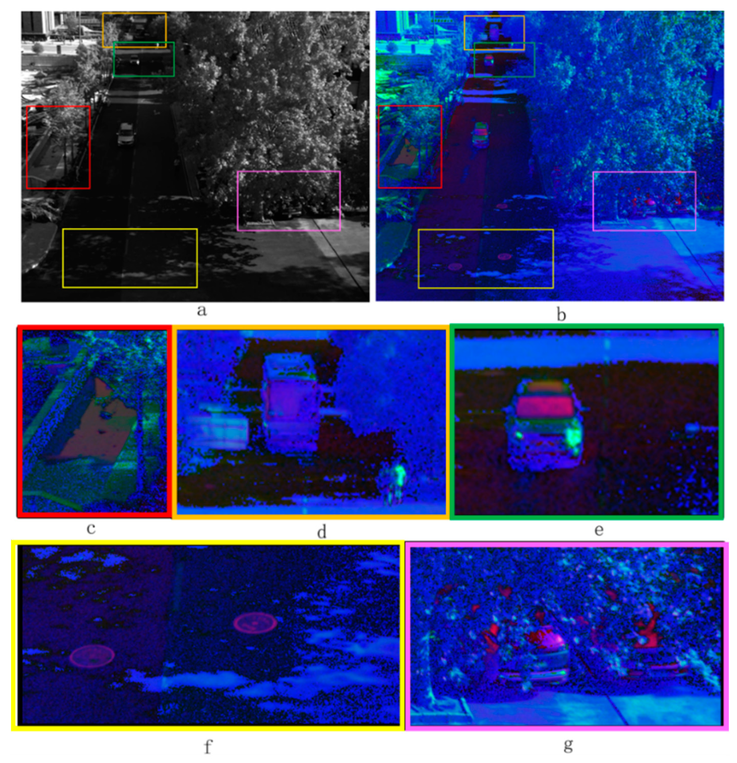
We conducted visual application experiments to demonstrate the importance and effectiveness of PIRC demosaicing. As the polarization reflection characteristics of the surfaces of different materials are varied, polarization imaging can serve visual tasks such as target detection and scene segmentation. Here, we focused on the potential of distinguishing objects by the difference in polarization characteristics and did not consider target detection or image segmentation algorithms.
Figure 5 show the pseudo-color images synthesized by the polarization images after PIRC demosaicing. The synthesis method directly normalized the calculated DOLP, AOPL, and I, and then filled them into the R, G, and B channels of the color image. This article provides a simple illustration of this process and does not discuss other more advanced fusion methods.
4. Discussion
In Table 1, Table 2, Table 3, Table 4, Table 5, Table 6, Table 7 and Table 8, the results show that our method and the EARI [29] method alternately achieved state-of-the-art performance, and both of them outperformed the other methods. Their performances varied on different datasets, which is mainly due to the different texture conditions of the experimental images.
In Table 9, for different algorithms, the results show that the improvement of the accuracy also brought an increase in the calculation time. Bilinear interpolation and bicubic interpolation were the fastest; in contrast, EARI and our PIRC took more time. However, PIRC was still considerably faster than EARI, although their accuracy was similar. In the experiments of this article, we did not do a special acceleration optimization for all of those algorithms. It is expected that our method can meet the needs of real-time applications after the necessary acceleration optimization.
Figure 5 is an outdoor scene. Figure 5a is the light intensity image, and Figure 5b is the pseudo-color image synthesized by polarization information. Figure 5c–g show the targets marked with colored boxes. They are water on the ground, buses, cars, sewer manhole covers, and cars hidden under the canopy, respectively. It can be observed that the targets that are difficult to distinguish in the light intensity image are clearly distinguished in the polarization information fusion image. For example, in Figure 5c, the surface of the stagnant water is smooth, and the specular reflection is obvious, thus the polarization characteristics are significantly different from the surrounding environment. In Figure 5e–g, the car’s glass and the manhole cover on the road are a red tone due to the strong degree of polarization. These polarization characteristics effectively aid in visual tasks, such as detecting, recognizing, and tracking vehicles by UAV, intersection monitoring, and detecting road surface water by unmanned vehicles.
5. Conclusions
This work presented a new polarized intensity ratio constraint demosaicing method for dividing a focal-plane polarimetric image. The method could efficiently utilize both the interchannel and intrachannel correlations and retain the characteristics of polarization detection. Our method first restored the light intensity image following the edge and texture. It then further restored the image of each channel according to the unique constraint relationship between the polarization channels. We directly used the mosaic image obtained by the DoFP sensor as the ground truth for the comparison experiment, which could greatly facilitate data collection and enrich the source of experimental data. The experimental results demonstrated our proposed method was both effective and practical. The findings also showed how polarimetric imaging could benefit computer vision and remote sensing tasks. In the future, we will continue to improve imaging quality. Other future research directions include multi-frame demosaicing, polarized 3D reconstruction, polarized target detection, and polarized target tracking.
Author Contributions
Conceptualization, K.J.; methodology, K.J.; software, K.J.; validation, Y.L.; formal analysis, L.Y.; investigation, K.J.; resources, H.Z.; data curation, R.Z. and K.J.; writing—original draft preparation, K.J.; writing—review and editing, Y.L.; visualization, H.Z.; supervision, L.Y.; project administration, L.Y.; funding acquisition, L.Y. and F.Z. All authors have read and agreed to the published version of the manuscript.
Funding
This research was funded by National Key R&D Program of China, grant number 2017YFB0503004 and 2017YFB0503003.
Data Availability Statement
The code is openly available at https://github.com/JKevinCH/PIRC (accessed on 16 April 2022).
Acknowledgments
Conflicts of Interest
The authors declare no conflict of interest.
Appendix A. Detailed Results for Each Image in All Datasets
Table 1, Table 2, Table 3, Table 4, Table 5, Table 6, Table 7 and Table 8 presented the average PSNR and CPSNR on each dataset. Here, Figure A1, Figure A2, Figure A3, Figure A4, Figure A5 and Figure A6 presented detailed results for each image in all datasets. The results show that our method and the EARI [29] method alternately achieved state-of-the-art performance.
Figure A1.
The PSNR of each image on the PSD [39] dataset.
Figure A1.
The PSNR of each image on the PSD [39] dataset.
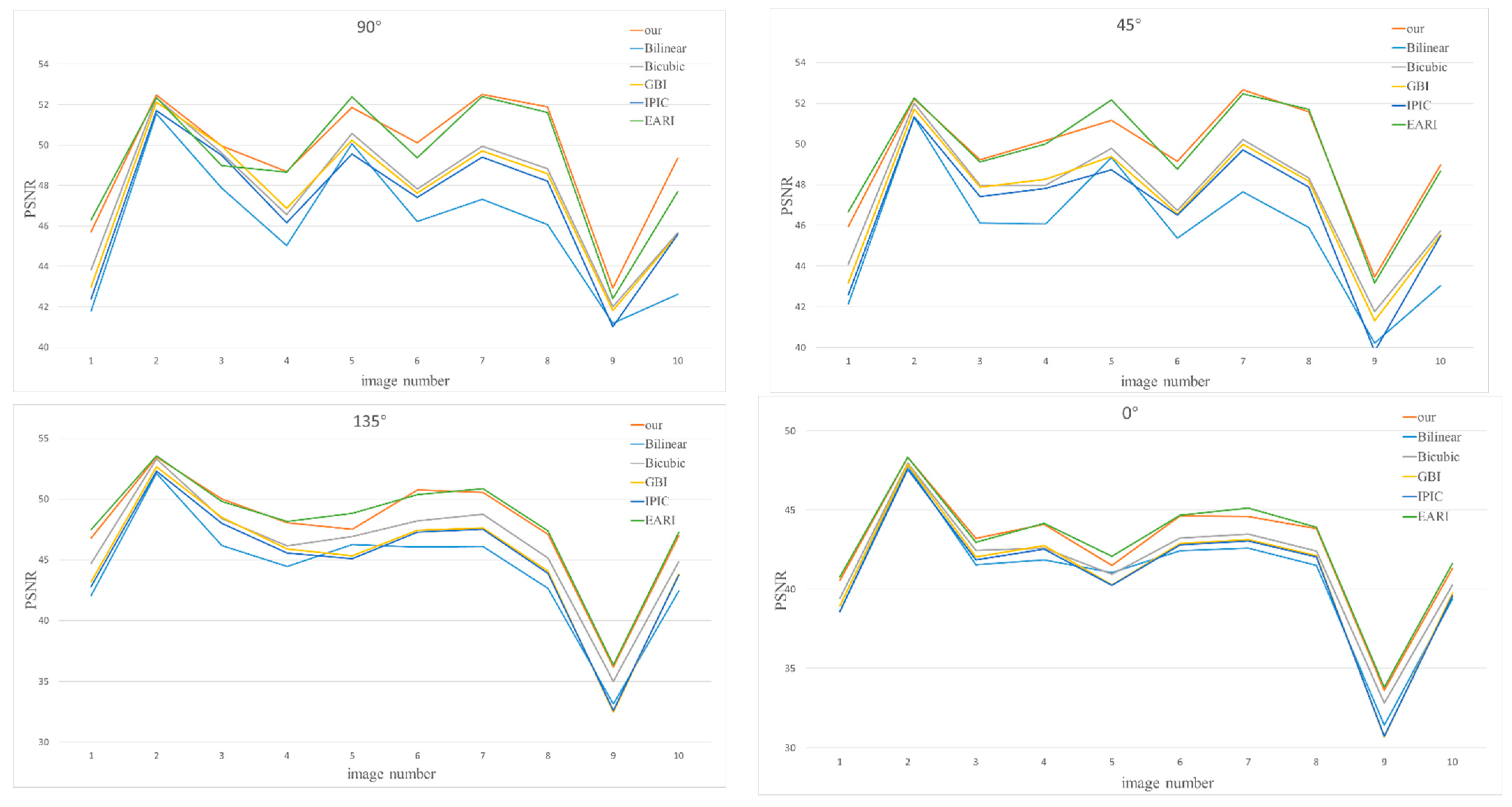
Figure A2.
The PSNR of each image on the JCPD [40] “indoor light” dataset.
Figure A2.
The PSNR of each image on the JCPD [40] “indoor light” dataset.

Figure A3.
The PSNR and CPSNR of each image on the JCPD [40] “polar light” dataset.
Figure A3.
The PSNR and CPSNR of each image on the JCPD [40] “polar light” dataset.

Figure A4.
The PSNR and CPSNR of each image on the Qiu [41] dataset.
Figure A4.
The PSNR and CPSNR of each image on the Qiu [41] dataset.

Figure A5.
The PSNR of each image on the EARI [29] dataset.
Figure A5.
The PSNR of each image on the EARI [29] dataset.

Figure A6.
The PSNR and CPSNR of each image on the “still” (number 1–7), “indoor” (number 8–12), and “outdoor” (number 8–17) datasets.
Figure A6.
The PSNR and CPSNR of each image on the “still” (number 1–7), “indoor” (number 8–12), and “outdoor” (number 8–17) datasets.

References
- Gurton, K.; Felton, M.; Mack, R.; LeMaster, D.; Farlow, C.; Kudenov, M.; Pezzaniti, L. MidIR and LWIR polarimetric sensor comparison study. In Proceedings of the SPIE Defense, Security, and Sensing, Orlando, FL, USA, 5–9 April 2010; Volume 7664. [Google Scholar]
- Zhou, Y.W.; Li, Z.F.; Zhou, J.; Li, N.; Zhou, X.H.; Chen, P.P.; Zheng, Y.L.; Chen, X.S.; Lu, W. High extinction ratio super pixel for long wavelength infrared polarization imaging detection based on plasmonic microcavity quantum well infrared photodetectors. Sci. Rep. 2018, 8, 15070. [Google Scholar] [CrossRef] [PubMed] [Green Version]
- Schechner, Y.Y.; Narasimhan, S.G.; Nayar, S.K. Polarization-based vision through haze. Appl. Opt. 2003, 42, 511–525. [Google Scholar] [CrossRef] [PubMed]
- Zhang, W.F.; Lang, J.; Ren, L.Y. Haze-removal polarimetric imaging schemes with the consideration of airlight’s circular polarization effect. Optik 2019, 182, 1099–1105. [Google Scholar] [CrossRef]
- Liu, F.; Han, P.L.; Wei, Y.; Yang, K.; Huang, S.Z.; Li, X.; Zhang, G.; Bai, L.; Shao, X.P. Deeply seeing through highly turbid water by active polarization imaging. Opt. Lett. 2018, 43, 4903–4906. [Google Scholar] [CrossRef] [PubMed]
- Reda, M.; Zhao, Y.; Chan, J.C.-W. Polarization Guided Autoregressive Model for Depth Recovery. IEEE Photon. J. 2017, 9, 6803016. [Google Scholar] [CrossRef]
- Kadambi, A.; Taamazyan, V.; Shi, B.; Raskar, R. Polarized 3D: High-Quality Depth Sensing with Polarization Cues. In Proceedings of the 2015 IEEE International Conference on Computer Vision (ICCV), Santiago, Chile, 7–13 December 2015; pp. 3370–3378. [Google Scholar]
- Gruev, V.; Perkins, R.; York, T. CCD polarization imaging sensor with aluminum nanowire optical filters. Opt. Express 2010, 18, 19087–19094. [Google Scholar] [CrossRef]
- Li, X.; Gunturk, B.; Zhang, L. Image demosaicing: A systematic survey. In Proceedings of the Electronic Imaging, San Jose, CA, USA, 27–31 January 2008; Volume 6822. [Google Scholar]
- Kiku, D.; Monno, Y.; Tanaka, M.; Okutomi, M. Minimized-Laplacian Residual Interpolation for Color Image Demosaicking. In Proceedings of the IS&T/SPIE Electronic Imaging, San Francisco, CA, USA, 2–6 February 2014; Volume 9023. [Google Scholar]
- Bayer, B.E. Color Imaging Array. U.S. Patent 3,971,065A, 5 March 1975. [Google Scholar]
- Rust, D.M. Integrated Dual Imaging Detector. U.S. Patent 5,438,414, 22 January 1995. [Google Scholar]
- Tokuda, T.; Sato, S.; Yamada, H.; Sasagawa, K.; Ohta, J. Polarisation-analysing CMOS photosensor with monolithically embedded wire grid polariser. Electron. Lett. 2009, 45, 228–229. [Google Scholar] [CrossRef]
- Brock, N.J.; Crandall, C.; Millerd, J.E. Snap-shot Imaging Polarimeter: Performance and Applications. In Proceedings of the SPIE Sensing Technology + Applications, Baltimore, MA, USA, 5–9 May 2014; Volume 9099. [Google Scholar]
- Mihoubi, S.; Lapray, P.-J.; Bigué, L. Survey of Demosaicking Methods for Polarization Filter Array Images. Sensors 2018, 18, 3688. [Google Scholar] [CrossRef] [Green Version]
- Paliy, D.; Katkovnik, V.; Bilcu, R.; Alenius, S.; Egiazarian, K. Spatially adaptive color filter array interpolation for noiseless and noisy data. Int. J. Imag. Syst. Tech. 2007, 17, 105–122. [Google Scholar] [CrossRef] [Green Version]
- Pekkucuksen, I.; Altunbasak, Y. Multiscale Gradients-Based Color Filter Array Interpolation. IEEE Trans. Image Process. 2013, 22, 157–165. [Google Scholar] [CrossRef]
- Kiku, D.; Monno, Y.; Tanaka, M.; Okutomi, M. Residual Interpolation for Color Image Demosaicking. In Proceedings of the 2013 20th IEEE International Conference on Image Processing (ICIP 2013), Melbourne, Australia, 15–18 September 2013; pp. 2304–2308. [Google Scholar]
- Alleysson, D.; Susstrunk, S.; Herault, J. Linear demosaicing inspired by the human visual system. IEEE Trans. Image Process. 2005, 14, 439–449. [Google Scholar] [PubMed] [Green Version]
- Dubois, E. Frequency-domain methods for demosaicking of Bayer-sampled color images. IEEE Signal Proc. Lett. 2005, 12, 847–850. [Google Scholar] [CrossRef]
- Leung, B.; Jeon, G.; Dubois, E. Least-Squares Luma-Chroma Demultiplexing Algorithm for Bayer Demosaicking. IEEE Trans. Image Process. 2011, 20, 1885–1894. [Google Scholar] [CrossRef] [PubMed]
- Mairal, J.; Elad, M.; Sapiro, G. Sparse representation for color image restoration. IEEE Trans. Image Process. 2008, 17, 53–69. [Google Scholar] [CrossRef] [Green Version]
- Moghadam, A.A.; Aghagolzadeh, M.; Kumar, M.; Radha, H. Compressive Framework for Demosaicing of Natural Images. IEEE Trans. Image Process. 2013, 22, 2356–2371. [Google Scholar] [CrossRef]
- Kokkinos, F.; Lefkimmiatis, S. Deep Image Demosaicking Using a Cascade of Convolutional Residual Denoising Networks. In Proceedings of the European Conference on Computer Vision, Munich, Germany, 8–14 September 2018; pp. 317–333. [Google Scholar]
- Gao, S.K.; Gruev, V. Bilinear and bicubic interpolation methods for division of focal plane polarimeters. Opt. Express 2011, 19, 26161–26173. [Google Scholar] [CrossRef]
- Gao, S.K.; Gruev, V. Gradient-based interpolation method for division-of-focal-plane polarimeters. Opt. Express 2013, 21, 1137–1151. [Google Scholar] [CrossRef]
- Zhang, J.C.; Luo, H.B.; Hui, B.; Chang, Z. Image interpolation for division of focal plane polarimeters with intensity correlation. Opt. Express 2016, 24, 20799–20807. [Google Scholar] [CrossRef]
- Wu, R.Y.; Zhao, Y.Q.; Li, N.; Kong, S.G. Polarization image demosaicking using polarization channel difference prior. Opt. Express 2021, 29, 22066–22079. [Google Scholar] [CrossRef]
- Morimatsu, M.; Monno, Y.; Tanaka, M.; Okutomi, M. Monochrome and Color Polarization Demosaicking Using Edge-Aware Residual Interpolation. In Proceedings of the 2020 IEEE International Conference on Image Processing (ICIP), Abu Dhabi, United Arab Emirates, 25–28 October 2020; pp. 2571–2575. [Google Scholar]
- He, K.M.; Sun, J.; Tang, X.O. Guided Image Filtering. IEEE Trans. Pattern Anal. Mach. Intell. 2013, 35, 1397–1409. [Google Scholar] [CrossRef]
- Ahmed, A.; Zhao, X.J.; Gruev, V.; Zhang, J.C.; Bermak, A. Residual interpolation for division of focal plane polarization image sensors. Opt. Express 2017, 25, 10651–10662. [Google Scholar] [CrossRef] [PubMed]
- Li, N.; Zhao, Y.Q.; Pan, Q.; Kong, S.G. Demosaicking DoFP images using Newton’s polynomial interpolation and polarization difference model. Opt. Express 2019, 27, 1376–1391. [Google Scholar] [CrossRef] [PubMed]
- Jiang, T.C.; Wen, D.S.; Song, Z.X.; Zhang, W.K.; Li, Z.X.; Wei, X.; Liu, G. Minimized Laplacian residual interpolation for DoFP polarization image demosaicking. Appl. Opt. 2019, 58, 7367–7374. [Google Scholar] [CrossRef]
- Liu, S.M.; Chen, J.J.; Xun, Y.; Zhao, X.J.; Chang, C.H. A New Polarization Image Demosaicking Algorithm by Exploiting Inter-Channel Correlations With Guided Filtering. IEEE Trans. Image Process. 2020, 29, 7076–7089. [Google Scholar] [CrossRef]
- Zhang, J.C.; Shao, J.B.; Luo, H.B.; Zhang, X.Y.; Hui, B.; Chang, Z.; Liang, R.G. Learning a convolutional demosaicing network for microgrid polarimeter imagery. Opt. Lett. 2018, 43, 4534–4537. [Google Scholar] [CrossRef]
- Wen, S.J.; Zheng, Y.Q.; Lu, F.; Zhao, Q.P. Convolutional demosaicing network for joint chromatic and polarimetric imagery. Opt. Lett. 2019, 44, 5646–5649. [Google Scholar] [CrossRef]
- Elad, M.; Aharon, M. Image denoising via sparse and redundant representations over learned dictionaries. IEEE Trans. Image Process. 2006, 15, 3736–3745. [Google Scholar] [CrossRef]
- Huang, L.; Xiao, L.; Wei, Z. A Nonlocal Sparse Representation Method for Color Demosaicking. Acta Electron. Sin. 2014, 42, 66–73. [Google Scholar]
- Lapray, P.J.; Gendre, L.; Foulonneau, A.; Bigue, L. A database of polarimetric and multispectral images in the visible and NIR regions. In Proceedings of the SPIE Photonics Europe, Strasbourg, France, 22–26 April 2018; Volume 10677. [Google Scholar]
- Mahalanobis, A.; Vijaya Kumar, B.V.K.; Juday, R.D. Correlation Pattern Recognition; Cambridge University Press: Cambridge, UK, 2005. [Google Scholar]
- Wen, S.; Zheng, Y.; Lu, F. A Sparse Representation Based Joint Demosaicing Method for Single-Chip Polarized Color Sensor. IEEE Trans. Image Process. 2021, 30, 4171–4182. [Google Scholar] [CrossRef]
- Qiu, S.M.; Fu, Q.; Wang, C.L.; Heidrich, W. Linear Polarization Demosaicking for Monochrome and Colour Polarization Focal Plane Arrays. Comput. Graph. Forum 2021, 40, 77–89. [Google Scholar] [CrossRef]
Figure 1.
Micropolarization array (a) and polarization of raw mosaic image (b).
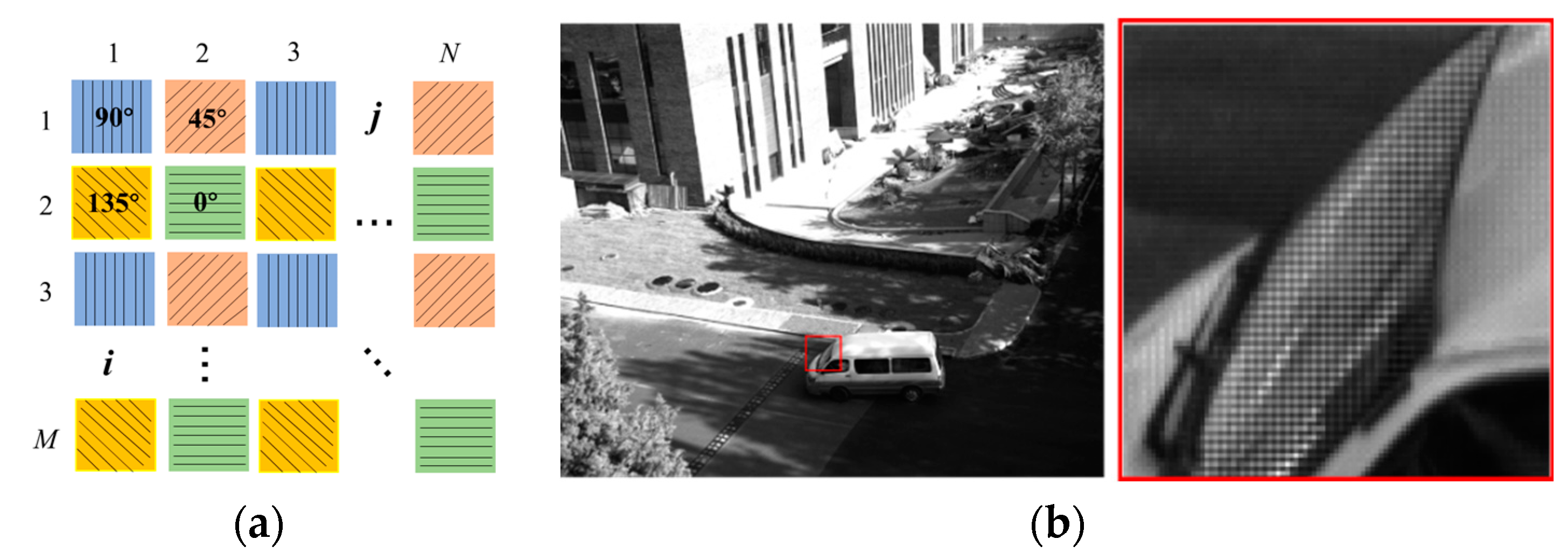
Figure 2.
PIRC demosaicing process.
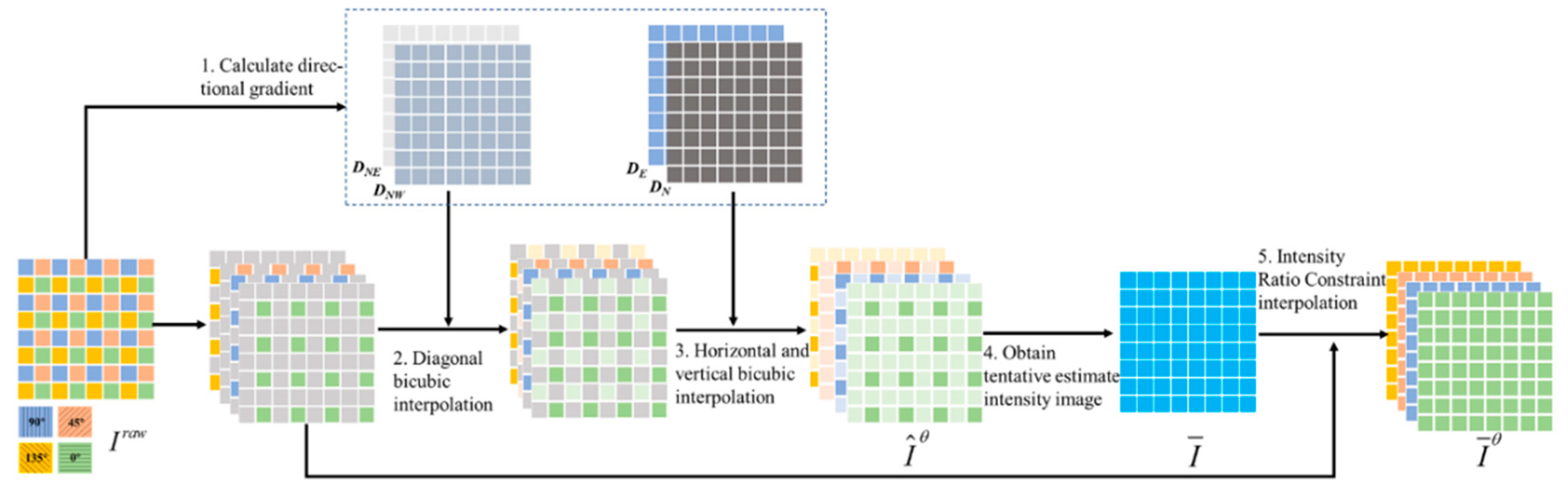
Figure 3.
Using a raw mosaic image as the ground truth for reference evaluation.

Figure 4.
Polarization image dataset collected by our DoFP polarization camera.
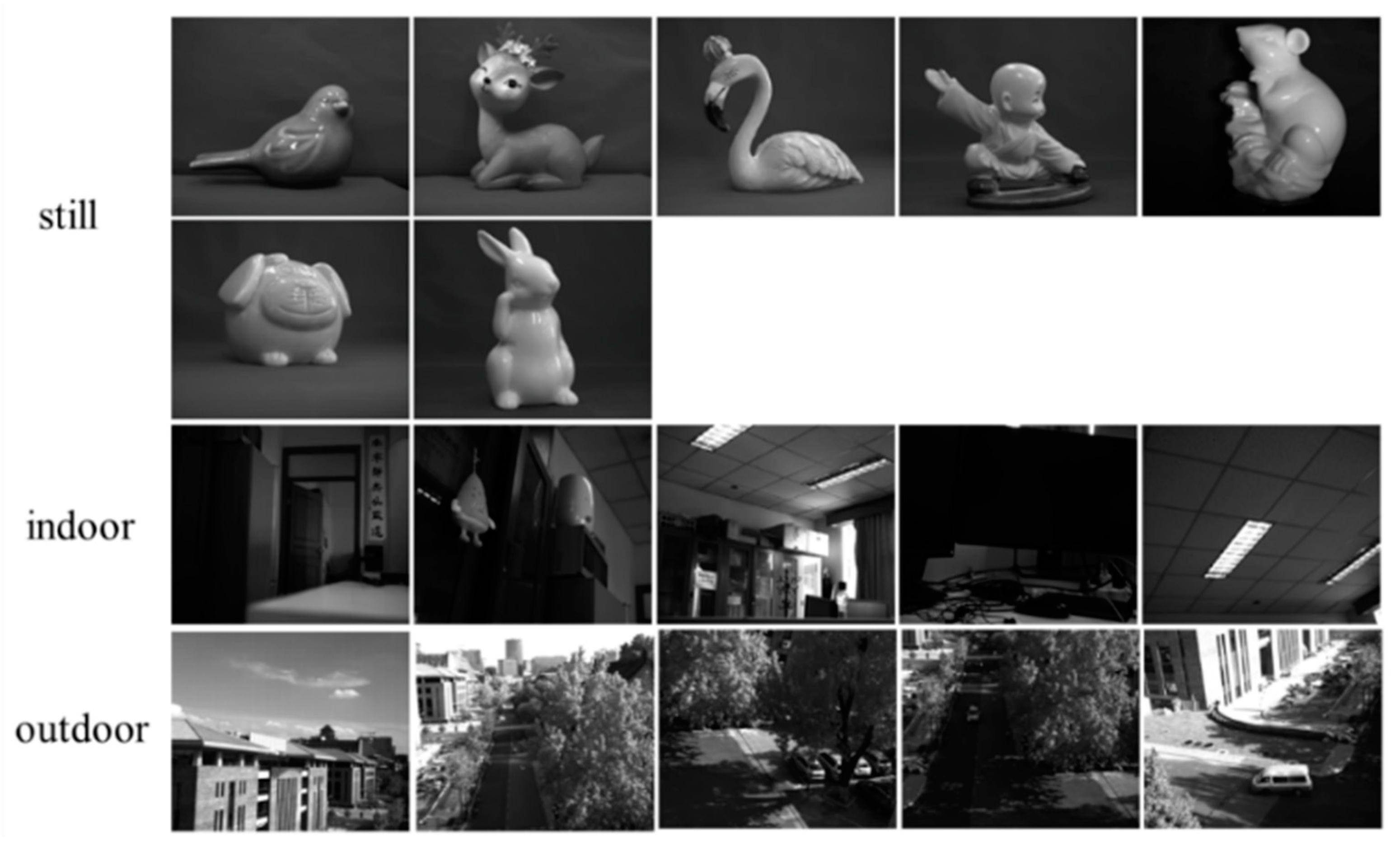
Figure 5.
Outdoor scene pseudo-color images synthesized by the polarization images after PIRC demosaicing. (a) is the light intensity image; (b) is the pseudo-color image synthesized by polarization information; (c–g) show the targets marked with colored boxes; they are water on the ground, buses, cars, sewer manhole covers, and cars hidden under the canopy, respectively.

Table 1.
The average PSNR and CPSNR of the comparative results on the PSD [39] dataset.
Table 1.
The average PSNR and CPSNR of the comparative results on the PSD [39] dataset.
| Bilinear | Bicubic | GBI | IPIC | EARI | Ours | ||
|---|---|---|---|---|---|---|---|
| PSNR | I90° | 45.9743 | 47.7189 | 47.5476 | 47.0923 | 49.2188 | 49.5521 |
| I0° | 45.7130 | 47.4576 | 47.2032 | 46.7278 | 49.4986 | 49.4521 | |
| I45° | 40.8210 | 41.5623 | 41.0495 | 40.9053 | 42.7548 | 42.5748 | |
| I135° | 44.1407 | 46.1404 | 45.0915 | 44.8752 | 48.0021 | 47.7359 | |
| I | 47.1367 | 48.9923 | 48.0670 | 48.0852 | 50.7618 | 50.5035 | |
| CPSNR | 44.0212 | 45.3788 | 44.7658 | 44.5683 | 46.8622 | 46.7302 | |
Table 2.
The average PSNR and CPSNR of the comparative results on the JCPD [41] “indoor light” dataset.
Table 2.
The average PSNR and CPSNR of the comparative results on the JCPD [41] “indoor light” dataset.
| Bilinear | Bicubic | GBI | IPIC | EARI | Ours | ||
|---|---|---|---|---|---|---|---|
| PSNR | I90° | 37.8308 | 39.0858 | 39.0689 | 38.8231 | 41.9451 | 42.5955 |
| I0° | 38.0426 | 39.2896 | 39.2959 | 39.0383 | 42.3034 | 42.1324 | |
| I45° | 38.0524 | 39.2908 | 39.3114 | 39.0639 | 41.8135 | 41.6400 | |
| I135° | 37.9027 | 39.1411 | 39.1632 | 38.9212 | 41.8940 | 41.6849 | |
| I | 41.0207 | 42.6195 | 42.2517 | 42.3376 | 45.6459 | 45.4912 | |
| CPSNR | 38.4160 | 39.6978 | 39.6642 | 39.4527 | 42.4921 | 42.3369 | |
Table 3.
The average PSNR and CPSNR of the comparative results on the JCPD [41] “polar light” dataset.
Table 3.
The average PSNR and CPSNR of the comparative results on the JCPD [41] “polar light” dataset.
| Bilinear | Bicubic | GBI | IPIC | EARI | Ours | ||
|---|---|---|---|---|---|---|---|
| PSNR | I90° | 43.3966 | 44.2719 | 44.4778 | 44.2141 | 45.3170 | 45.9523 |
| I0° | 41.8220 | 42.8536 | 43.0237 | 42.8074 | 44.2339 | 44.4133 | |
| I45° | 40.2640 | 41.2586 | 41.0635 | 41.0114 | 41.7744 | 42.1586 | |
| I135° | 42.2719 | 43.3034 | 43.4551 | 43.1951 | 44.4374 | 44.6750 | |
| I | 45.4879 | 46.8313 | 46.6407 | 46.6710 | 47.9939 | 48.3255 | |
| CPSNR | 42.2504 | 43.2872 | 43.2981 | 43.1510 | 44.2396 | 44.5935 | |
Table 4.
The average PSNR and CPSNR of the comparative results on the Qiu [42] dataset.
Table 4.
The average PSNR and CPSNR of the comparative results on the Qiu [42] dataset.
| Bilinear | Bicubic | GBI | IPIC | EARI | Ours | ||
|---|---|---|---|---|---|---|---|
| PSNR | I90° | 45.4405 | 45.9100 | 46.1176 | 45.8781 | 47.7405 | 47.7238 |
| I0° | 45.1386 | 45.5986 | 45.8165 | 45.5700 | 47.5268 | 47.4604 | |
| I45° | 43.8359 | 44.2798 | 44.4799 | 44.2611 | 46.3113 | 46.1561 | |
| I135° | 44.1497 | 44.5925 | 44.8264 | 44.5903 | 46.7437 | 46.4882 | |
| I | 47.5776 | 48.2071 | 48.2397 | 48.2368 | 50.2006 | 50.0745 | |
| CPSNR | 44.7896 | 45.2569 | 45.4470 | 45.2367 | 47.2583 | 47.1266 | |
Table 5.
The average PSNR and CPSNR of the comparative results on the EARI [29] dataset.
Table 5.
The average PSNR and CPSNR of the comparative results on the EARI [29] dataset.
| Bilinear | Bicubic | GBI | IPIC | EARI | Ours | ||
|---|---|---|---|---|---|---|---|
| PSNR | I90° | 42.5052 | 43.6349 | 43.5218 | 43.1572 | 46.8653 | 46.5659 |
| I0° | 41.5901 | 42.4932 | 42.4689 | 42.0089 | 44.5156 | 44.5318 | |
| I45° | 42.3522 | 43.4642 | 43.3320 | 42.9762 | 46.5403 | 46.2573 | |
| I135° | 41.5906 | 42.4905 | 42.4565 | 42.0234 | 44.3447 | 44.3395 | |
| I | 44.9012 | 46.2316 | 45.7717 | 45.7528 | 48.9070 | 48.7685 | |
| CPSNR | 42.4162 | 43.4488 | 43.3319 | 42.9681 | 45.8718 | 45.7766 | |
Table 6.
The average PSNR and CPSNR of the comparative results on the “still” dataset.
| Bilinear | Bicubic | GBI | IPIC | EARI | Ours | ||
|---|---|---|---|---|---|---|---|
| PSNR | I90° | 42.6294 | 42.7586 | 43.1299 | 42.7421 | 43.3345 | 43.5794 |
| I0° | 42.6440 | 42.7406 | 43.1475 | 42.7236 | 43.3126 | 43.5161 | |
| I45° | 42.3462 | 42.4418 | 42.8330 | 42.4047 | 43.0599 | 43.2954 | |
| I135° | 42.2083 | 42.3328 | 42.7339 | 42.3044 | 42.9512 | 43.1924 | |
| I | 46.7591 | 47.2200 | 47.5390 | 47.2189 | 47.6745 | 48.0496 | |
| CPSNR | 43.0325 | 43.1731 | 43.5595 | 43.1493 | 43.7586 | 44.0018 | |
Table 7.
The average PSNR and CPSNR of the comparative results on the “indoor” dataset.
| Bilinear | Bicubic | GBI | IPIC | EARI | Ours | ||
|---|---|---|---|---|---|---|---|
| PSNR | I90° | 42.0446 | 42.7083 | 43.1710 | 42.9867 | 43.4097 | 43.9911 |
| I0° | 42.7276 | 43.3628 | 43.8270 | 43.6124 | 44.3127 | 44.6737 | |
| I45° | 43.3046 | 43.9254 | 44.4055 | 44.1752 | 44.7508 | 45.1523 | |
| I135° | 42.4136 | 43.0817 | 43.5635 | 43.3420 | 43.8367 | 44.3540 | |
| I | 46.3890 | 47.4204 | 47.9224 | 47.7924 | 48.1915 | 48.8117 | |
| CPSNR | 43.1252 | 43.8093 | 44.2832 | 44.0801 | 44.6053 | 45.0960 | |
Table 8.
The average PSNR and CPSNR of the comparative results on the “outdoor” dataset.
| Bilinear | Bicubic | GBI | IPIC | EARI | Ours | ||
|---|---|---|---|---|---|---|---|
| PSNR | I90° | 28.1875 | 28.4304 | 28.3835 | 27.9342 | 29.6191 | 29.4768 |
| I0° | 29.1214 | 29.3598 | 29.3973 | 28.9050 | 30.4234 | 30.3209 | |
| I45° | 28.7657 | 29.0162 | 29.0302 | 28.5602 | 30.2432 | 30.0793 | |
| I135° | 27.7849 | 28.0249 | 27.9010 | 27.4841 | 29.1247 | 28.9946 | |
| I | 31.6101 | 32.0732 | 31.7485 | 31.5990 | 33.2384 | 33.0928 | |
| CPSNR | 28.9001 | 29.1659 | 29.0954 | 28.6748 | 30.3123 | 30.1762 | |
Table 9.
Comparison of time cost.
| Image Size | Processing Time(s) | |||||
|---|---|---|---|---|---|---|
| Bilinear | Bicubic | GBI | IPIC | EARI | Ours | |
| 1244 × 1024 | 0.0737 | 0.0949 | 0.2542 | 0.3357 | 2.0328 | 1.3846 |
| 1024 × 1024 | 0.0613 | 0.0800 | 0.2190 | 0.2777 | 1.7020 | 1.1751 |
| 1024 × 768 | 0.0444 | 0.0595 | 0.1856 | 0.2319 | 1.2074 | 0.8586 |
| 720 × 540 | 0.0222 | 0.0286 | 0.0794 | 0.1021 | 0.5698 | 0.4334 |
Table 10.
The average PSNR and CPSNR of the controlled experiment results on the PSD [39] dataset.
Table 10.
The average PSNR and CPSNR of the controlled experiment results on the PSD [39] dataset.
| PSNR | CPSNR | |||||
|---|---|---|---|---|---|---|
| I90° | I0° | I45° | I135° | I | ||
| 0 | 49.4534 | 49.2667 | 42.4710 | 47.5507 | 50.3324 | 46.6011 |
| 0.001 | 49.5673 | 49.4367 | 42.5582 | 47.7009 | 50.4826 | 46.7139 |
| 0.005 | 49.5521 | 49.4521 | 42.5748 | 47.7359 | 50.5035 | 46.7302 |
| 0.01 | 49.4934 | 49.4143 | 42.5702 | 47.7339 | 50.4982 | 46.7172 |
| 0.1 | 49.4406 | 49.3700 | 42.5614 | 47.7119 | 50.4832 | 46.6978 |
| 1 | 49.3792 | 49.3305 | 42.5566 | 47.7177 | 50.4820 | 46.6857 |
| 10 | 49.3490 | 49.3045 | 42.5505 | 47.6994 | 50.4708 | 46.6724 |
| 100 | 49.3595 | 49.3158 | 42.5539 | 47.7150 | 50.4789 | 46.6801 |
Table 11.
The results of the original guided filter with different ε on the PSD [33] dataset.
Table 11.
The results of the original guided filter with different ε on the PSD [33] dataset.
| PSNR | CPSNR | |||||
|---|---|---|---|---|---|---|
| I90° | I0° | I45° | I135° | I | ||
| 0 | 45.5900 | 45.7077 | 42.2698 | 45.7752 | 48.2528 | 45.0309 |
| 0.001 | 45.5987 | 45.7166 | 42.2721 | 45.7821 | 48.2603 | 45.0367 |
| 0.01 | 45.6763 | 45.7954 | 42.2918 | 45.8434 | 48.3269 | 45.0881 |
| 0.05 | 46.0070 | 46.1320 | 42.3697 | 46.0980 | 48.6067 | 45.3019 |
| 0.1 | 46.3239 | 46.4516 | 42.4275 | 46.3039 | 48.8561 | 45.4872 |
| 1 | 48.8572 | 48.9465 | 42.4346 | 47.3465 | 50.2805 | 46.4396 |
| 10 | 47.5377 | 47.2827 | 41.4780 | 45.6522 | 48.5795 | 45.1483 |
| 100 | 46.6212 | 46.3342 | 41.0616 | 44.7765 | 47.7319 | 44.4821 |
Publisher’s Note: MDPI stays neutral with regard to jurisdictional claims in published maps and institutional affiliations. |
© 2022 by the authors. Licensee MDPI, Basel, Switzerland. This article is an open access article distributed under the terms and conditions of the Creative Commons Attribution (CC BY) license (https://creativecommons.org/licenses/by/4.0/).
Share and Cite
MDPI and ACS Style
Yan, L.; Jiang, K.; Lin, Y.; Zhao, H.; Zhang, R.; Zeng, F. Polarized Intensity Ratio Constraint Demosaicing for the Division of a Focal-Plane Polarimetric Image. Remote Sens. 2022, 14, 3268. https://doi.org/10.3390/rs14143268
AMA Style
Yan L, Jiang K, Lin Y, Zhao H, Zhang R, Zeng F. Polarized Intensity Ratio Constraint Demosaicing for the Division of a Focal-Plane Polarimetric Image. Remote Sensing. 2022; 14(14):3268. https://doi.org/10.3390/rs14143268
Chicago/Turabian StyleYan, Lei, Kaiwen Jiang, Yi Lin, Hongying Zhao, Ruihua Zhang, and Fangang Zeng. 2022. "Polarized Intensity Ratio Constraint Demosaicing for the Division of a Focal-Plane Polarimetric Image" Remote Sensing 14, no. 14: 3268. https://doi.org/10.3390/rs14143268
Note that from the first issue of 2016, this journal uses article numbers instead of page numbers. See further details here.