Article

Seasonal Variability in Chlorophyll and Air-Sea CO2 Flux in the Sri Lanka Dome: Hydrodynamic Implications

1
State Key Laboratory of Satellite Ocean Environment Dynamics, Second Institute of Oceanography, Ministry of Natural Resources, Hangzhou 310012, China
2
Southern Marine Science and Engineering Guangdong Laboratory (Zhuhai), Zhuhai 519000, China
3
State Key Laboratory of Loess and Quaternary Geology, Institute of Earth Environment, Chinese Academy of Sciences, Xi’an 710061, China
4
School of Oceanography, Shanghai Jiao Tong University, Shanghai 200240, China
*
Author to whom correspondence should be addressed.
Remote Sens. 2022, 14(14), 3239; https://doi.org/10.3390/rs14143239
Submission received: 23 May 2022 / Revised: 14 June 2022 / Accepted: 30 June 2022 / Published: 6 July 2022

Abstract

:
Multiple upwelling systems develop in the Indian Ocean during the summer monsoon. The Sri Lanka dome (SLD), which occurs in the open ocean off the east coast of Sri Lanka from June to September, is distinct from those near the coast. The SLD is characterized by uplifted thermocline and increased chlorophyll concentration. Mechanisms of the upwelling and its biogeochemical response are not well understood. Here, we explored the dynamics of the chlorophyll and sea-to-air CO2 flux in the SLD using ocean color and altimetry remote sensing data, together with other reanalysis products. We found that the occurrence of high chlorophyll concentration and sea-to-air CO2 flux happens along the pathway of the southwest monsoon current (SMC). The annual cycle of chlorophyll in the SLD has a one-month lag relative to that in the southern coast of Sri Lanka. The positive wind stress curl that forms in the SLD during the summer does not fully explain the seasonal chlorophyll maximum. Transport of the SMC, eddy activity, and associated frontal processes also play an important role in regulating the variability in chlorophyll. In the SLD, upwelled subsurface water has excess dissolved inorganic carbon (DIC) relative to the conventional Redfield ratio between DIC and nutrients; thus, upwelling and sub-mesoscale processes determine this region to be a net carbon source to the atmosphere.

1. Introduction

The Indian Ocean has a unique land–sea distribution characterized by the vast landmass located to the north of the ocean. Differential heating of land and sea results in a prominent monsoon climate [1,2]. The seasonal reversal of wind produces important upwelling systems in several parts of the Indian Ocean boundaries ranging from the west to the east [3,4] (Figure 1). The southwesterlies during boral summer are favorable for upwelling along the western boundary of the Arabian Sea, near the coast of Somalia and Oman [5,6,7,8,9]. In the eastern boundary of the Arabian Sea, the southwesterly winds turn mainly into onshore equatorward winds along the southwest coast of India, generating offshore Ekman transport and coastal upwelling [10,11]. In the eastern equatorial Indian Ocean, the southeasterlies along the southern coast of Java and Sumatra islands induces upwelling off the coast [12,13]. These boundary upwelling systems are mainly characterized as offshore transport of surface water where the subsurface water upwells to the surface. Subsequently, upwelled water with higher nutrients supports the high primary productivity and pelagic fisheries [14,15].
A seasonal upwelling also appears off the east coast of Sri Lanka (5–10°N, 83–87°E) during the southwest (SW) monsoon (June–September), known as the Sri Lanka dome (SLD) [16,17]. The SLD is a unique upwelling system that occurs in the open ocean. It starts in May, matures in July, and disappears in September [18]. The mechanism is different from other upwelling systems in the western Arabian Sea, the southwest coast of India, and the eastern equatorial Indian Ocean. The SW summer monsoon produces positive wind stress curl above the region of SLD and favors the upwelling via Ekman pumping [16]. A previous study using numerical model found that the existence of Sri Lanka island forces a strong surface current, namely, the southwest monsoon current (SMC) [17] which flows eastward from the eastern Arabian Sea to the Bay of Bengal (BoB) and finally turns northwestward after passing the south of Sri Lanka [19]. The anticlockwise turning of the SMC favors the occurrence of a cyclonic eddy (CE) to the east of Sri Lanka (Figure 1) [17,20]. Therefore, it is considered that the island mass effect, a phenomenon of increased chlorophyll near an island [21], and wind-driven Ekman pumping are thought to determine the existence and strength of the SLD, respectively. The dissipation of the SLD is attributed to the westward propagation of Rossby (downwelling) waves, which are associated with the reflection of the spring Wyrtki jet at the eastern boundary of the Indian Ocean [18,22,23].
The formation of the SLD introduces a prominent impact on the biogeochemical tracers as well. Remote sensing of ocean color shows increased chlorophyll in the surface waters of the SLD during the SW monsoon [24]. This is mainly because the upwelling breaks the strong stratification (the existence of a barrier layer) during summer and provides more nutrients to the surface [24,25,26,27,28]. However, the Bay of Bengal Boundary Layer Experiment (BoBBLE) showed a very low nutrient concentration in the SLD via ship-bound measurements [25,29]. This discrepancy was assumed due to the upwelled nutrient being rapidly consumed by phytoplankton in the surface [25]. Additionally, SMC is considered to transport water with high-chlorophyll to the SLD region from the south of Sri Lanka [20,24]. Due to the corresponding Ekman pumping, there are also prominent deep chlorophyll maxima (DCM) at intermediate depths (20–50 m) in the region of the SLD and the SMC [30]. Outside the dome, the DCM is weaker. Seasonal variations in chlorophyll in surface and subsurface waters have been linked to monsoon-regulated upwelling [31]. However, the detailed interaction between the region of SLD and south of Sri-Lanka is still not well understood.
Following the high chlorophyll concentration and net primary productivity (NPP), the biogenic CO2 uptake is enhanced as well. Numerical studies indicate that the enhanced NPP overcomes the upwelled water with high pCO2, resulting in a net carbon sink in the SLD [26,32]. However, the recent observation argues that the strong upwelling makes the SLD a net carbon source [25]. In recent years, the application of seawater pCO2 remote sensing provides a novel means to estimate the global and regional air–sea CO2 flux with higher spatial and temporal resolution than the conventional shipboard observation [33,34,35,36,37]. Relative to the upwelling system of the western Arabian Sea, physical and biological governing factors controlling seawater pCO2 in the SLD are not well understood.
In this study, we revisited the dynamics of the high chlorophyll concentration in the SLD. In addition to the wind stress curl induced upwelling, the strengthening and transport of SMC, a cyclonic–anticyclonic eddy dipole, and associated frontal process also play important roles. Furthermore, by calculating the seasonal variability of the sea-to-air CO2 flux in the southwestern BoB using the remote sensing and reanalysis products, our data support that the SLD is a net carbon source to the atmosphere.

2. Data and Methods

2.1. Datasets

(a) Monthly and 5-day gridded data of chlorophyll-a concentration in the SLD provided by the Ocean Colour Climate Change Initiative (Ocean Color CCI) v5.0 over the period from 1998 to 2020 were obtained from European Space Agency (ESA; https://www.oceancolour.org, accessed on 30 January 2022). The Ocean Color CCI is producing long-term multi-sensor timeseries of satellite ocean-color data with a horizontal resolution of 4.5 km [38]. Meanwhile, the monthly remote-sensing reflectance (Rrs) at the 443 nm, 488 nm, and 555 nm bands were also used to calculate the air–sea CO2 flux described in Section 2.4.
(b) The monthly reanalysis product of sea surface salinity (SSS) and mixed layer depth (MLD) were obtained from the E.U. Copernicus Marine Service (https://www.marine.copernicus.eu, accessed on 30 January 2022) to calculate the air–sea CO2 flux described in Section 2.4.
(c) Daily and monthly sea surface height anomaly (SSHA) and surface geostrophic current data, with a horizontal resolution of 0.25° over the same period as the chlorophyll-a data, were obtained from the E.U. Copernicus Marine Service. The product is processed by the DUACS data processing system from all altimeter missions: Jason-3, Sentinel-3A, HY-2A, Saral/AltiKa, Cryosat-2, Jason-2, Jason-1, T/P, ENVISAT, GFO, and ERS1/2.
(d) Mesoscale Eddy Trajectory Atlas products (META3.1exp DT) over the same period with chlorophyll-a concentration, processed by Centre National D’Etudes Spatiales/Collecte Localisation Satellites (CNES/CLS) in the DUACS system, were obtained from AVISO+ (https://www.aviso.altimetry.fr, accessed on 30 January 2022). All eddies with a lifetime greater than 8 days were extracted.
(e) The six-hourly near-surface (10 m) wind speed over the same period with chlorophyll-a concentration was obtained from the fifth-generation European Centre for Medium-Range Weather Forecasts (ECMWF) reanalysis (ERA5) dataset (http://cds.climate.copernicus.eu, accessed on 30 January 2022). The wind stress and its curl are derived from the wind speed. Here, wind stress is calculated as the function τ = Cd × ρ × u10, where τ is the wind stress, Cd is the drag coefficient, ρ is the density of air, and u10 is the wind speed at 10 m. Cd and ρ were set to 1.25 × 10⁻³ and 1.225 kg m−3, respectively. Wind stress curl is calculated as ∂τy/∂x − ∂τx/∂y, where τx and τy denote the wind stress in the x and y directions, respectively, that induces the vertical movement of the water mess via Ekman pumping [39].
(f) Daily sea surface temperature (SST) data with a horizontal resolution of 4.5 km for the period of 2003–2020 were obtained from NASA’s Moderate Resolution Imaging Spectroradiometer (MODIS) on Auqa (http://oceandata.sci.gsfc.nasa.gov, accessed on 30 January 2022) to perform the front detection.
(g) HYCOM reanalysis products of expt_57.2 (https://www.hycom.org, accessed on 10 February 2022), which has a horizontal resolution of ~0.08° (9 km) and 41 vertical layers, were obtained for the summer of 2016 with a time interval of 3 h. The HYCOM model uses the Navy Coupled Ocean Data Assimilation (NCODA) system for data assimilation. As most of the available satellite altimetry observations are assimilated in the NCODA, the modeled sea surface height and eddy locations are consistent with altimetry observations.

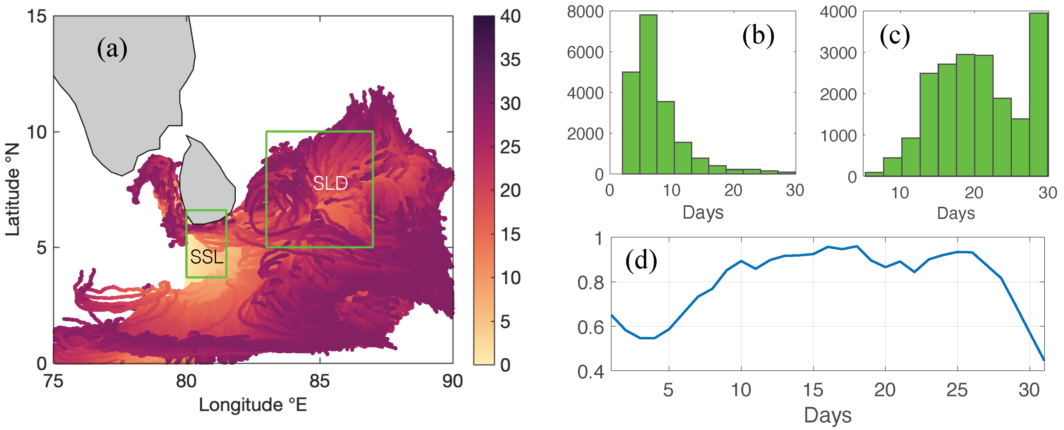
2.2. Lagrangian Particle Tracking

The motion of particles was tracked using the HYCOM current field. This method was used for the backward tracking of settling particles collected by the timeseries sediment trap in the South China Sea [40]. The motion of a particle is described by its position vector, X ( t ) , at time t . The velocity of the particle is interpolated from the HYCOM velocity outputs by setting the velocity in the Lagrangian frame equal to the velocity U ( x , t ) in the Eulerian frame when X ( a , t ) is crossing the point x:
( X ( a , t ) t ) a = U ( x , t )   where   X ( a , t ) = x ,
When the virtual particle is located at point X ( n ) ( t )   = x, we can update its position by a time step, t , to estimate the displacement:
X ( t + t ) = X ( t ) + t t + t v ( x , τ ) d τ
We simulated the general trajectory X ( t ) of particles by combining the Brownian motion, the drift following the current:
d X i ( t ) = a i ( X , t ) + σ i j ( x , t ) d W j ( t )
where X i ( t ) is the trajectory vector of a specific particle “i”, and d X i ( t ) = X i ( t + d t ) X i ( t ) is the stochastic particle displacement during the time interval [t, t + dt]. The term a i ( X , t ) is a deterministic drift, σ i j ( x , t ) is related to a diffusion tensor, and W j ( t ) is a Wiener process to represent the random walk realized by applying a perturbation to the velocity field. The horizontal and vertical diffusivity was set to 50 and 10−4 m2 s−2, respectively. The vertical water velocity is derived using the continuity equation. The particle itself does not have an active settling velocity in this study.

2.3. Front Detection

The SST front was detected using the gradient-based edge-detection method following refs. [39,41]. In the first step, the local maximum gradient was calculated. A patch was marked as frontal pixels if they had the gradient greater than a defined threshold of T1. In the next step, the position of the front filament was identified if the value of the gradient for adjacent pixels was larger than a threshold of T2 in the direction perpendicular to the gradient. This procedure repeated until the entire front filament was completed when the gradients for all surrounding pixels were smaller than T2. In this study, the thresholds of 2.8 °C and 1.4 °C per 100 km for T1 and T2, respectively, were adopted from the former study conducted in the Arabian Sea [41]. Different values of thresholds of T1 and T2 were tested to ensure the robustness of the detection. After the daily SST front was obtained, the frontal probability (FP) at each pixel was calculated in each month. The FP was defined as the ratio between the total number of times the pixel was identified as a front within the month and the number of times the pixel was cloud-free during the same time.

2.4. Remote Sensing of Sea-to-Air CO2 Flux

The remote sensing of seawater pCO2 is derived from satellite products including the remote-sensing reflectance (Rrs at 443 nm, 488 nm and 555 nm bands) and chlorophyll, as well as other reanalysis products such as the SST, SSS, and MLD (Table 1). Extreme gradient boosting (XGBoost) [42], a machine learning algorithm, was applied to create monthly sea surface pCO2 maps with a spatial resolution of 4.5 km for the period of 2003–2019 over the global ocean. Observed pCO2 data from the Surface Ocean Carbon Atlas (SOCAT) database [43] were used for training and validation. In this study, the SOCAT v3 data for the period of 2000–2015 was used for training, and the period of 2016–2018 was applied for validation. There are 792 stations in the central and eastern Indian Ocean used for training (Figure S1). After the seawater pCO2 was derived, we computed the air-to-sea CO2 flux using the approach of ref. [33]. The input variables to calculate the flux are described in Table 1.

3. Results

3.1. Chlorophyll

The remote sensing chlorophyll in the southwestern BoB shows a clear seasonal variability with high concentration during the SW summer monsoon and low value in the northeast winter monsoon (Figure 2). The summer high value occurs around the coast of south India and Sri Lanka (Figure 2b). There exists an offshore high chlorophyll patch distributed along the wind direction off the east coast of Sri Lanka. Meanwhile, this patch can be traced upstream to the south of Sri Lanka (SSL). In comparison, high chlorophyll during winter is only limited to the coastal regions around India and Sri Lanka, and the channel between them (Figure 2a). Monthly climatology of chlorophyll and wind stress curl averaged in the SLD and SSL also show prominent seasonal variability with high values during SW monsoon (Figure 3). The chlorophyll in SSL is persistently larger than that in SLD. The chlorophyll in SSL is increasing by almost four times from its lowest value to the largest value; in comparison, the increase is only twice in the SLD (Figure 3a). Consistently, the change in wind stress curl is also more prominent in SSL than that in SLD (Figure 3b). The monthly climatology of chlorophyll in the SLD and SSL shows that their maxima both occur during the SW monsoon, but the SSL leads SLD for one month (Figure 3a).

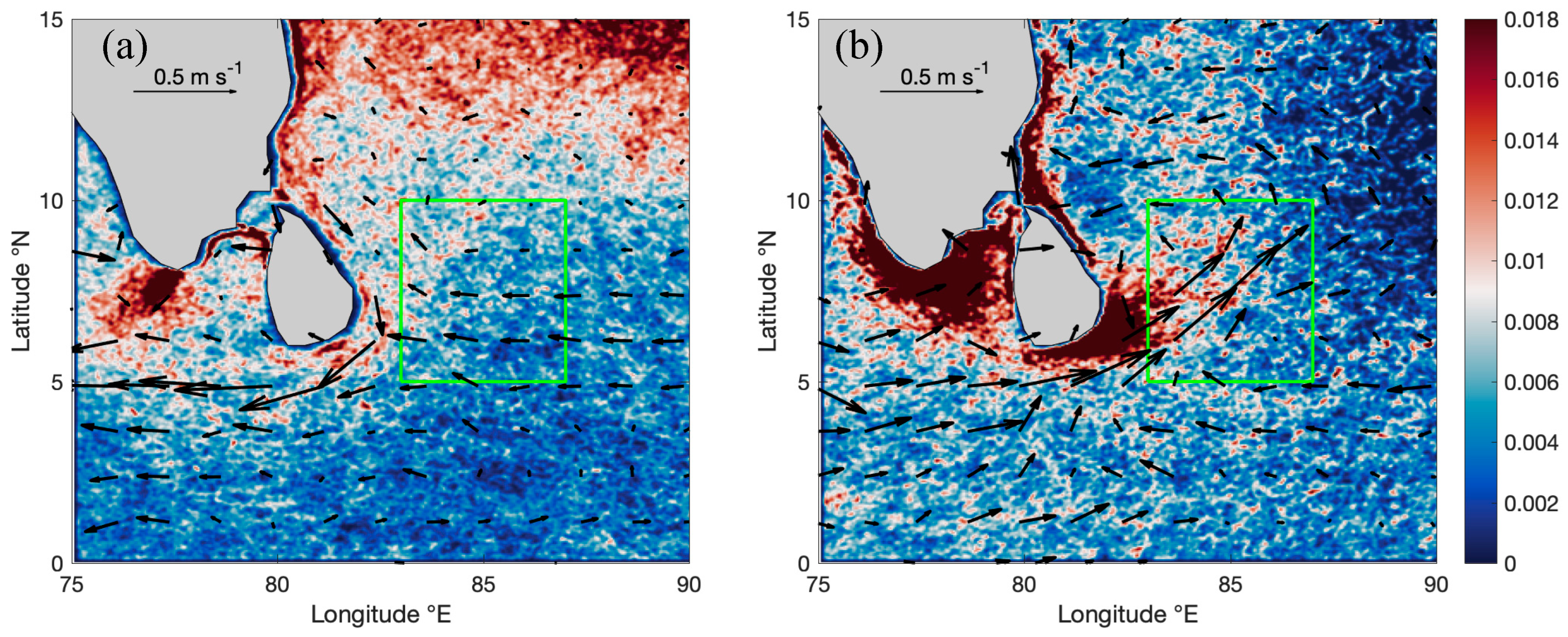
3.2. Wind Stress Curl

The positive and negative wind stress curls impose an upward and downward Ekman pumping to the ocean, respectively [44]. In the center of the SLD, a positive wind stress curl happens during summer (Figure 4a). The result is consistent with that of the cross-calibrated multiplatform (CCMP) wind product [45] (Figure S2). The position of the high chlorophyll patch (blue contour) generally matches the core of the positive wind stress curl stripe in the SLD region (Figure 4a). However, the monthly climatology of the wind stress curl in the SLD box shows significantly less seasonality than in the SSL box (Figure 3b). The wind stress curl in the SSL box shows positive values in summer (with a peak in July) and negative values in winter. In the SLD box, the value of the wind stress curl is positive throughout the year. The SLD box has two positive peaks in both winter and summer, but the summer peak in July is not significantly higher than the winter peak in December. The chlorophyll in the SLD box, however, is significantly lower in winter.

3.3. Sea Surface Height

The distribution of sea surface height anomaly (SSHA) in the SLD box shows a negative center in the northwest and a positive anomaly in the southeast (Figure 4b). This pattern is consistent with the result of the dome tracing result in which the dome is developed on the lee side of Sri Lanka, to the northwest of the SMC [46]. The counterclockwise pattern of the geostrophic current is consistent with the negative SSHA that usually favors upwelling in the coastal ocean [47,48,49]. However, the summer high chlorophyll patch does not match the negative SSHA region. Instead, a high chlorophyll patch occurs at the boundary between the negative and positive anomalies of SSHA, which denotes the maximum slope of SSHA and matches the position of the SMC.
The timeseries of SSHA in the SLD box show a long-term increasing trend (Figure S3), which is removed as the detrended SSHA (SSHAdetrend) before comparing with the chlorophyll. Most chlorophyll peaks in each year correspond to a negative SSHAdetrend and the R between them is −0.34. However, the SSHAdetrend shows variability with a higher frequency than the chlorophyll (Figure 5).
We applied the empirical orthogonal function (EOF) analysis to the monthly mean SSHAdetrend data in the region of 5–15°N, 75–90°E. The first principal component (PC1) interprets ~30% of the total variance and its distribution shows a dipole with the boundary near the SMC (Figure 6a). PC2 accounts for ~20% of the total variance (Figure 6b). It shows the antiphase of the core of the high chlorophyll patch in the SLD and the east coast of south India relative to other regions. PC3 shows a dipole pattern in the region off the east coast of Sri Lanka (Figure 6c). PC4 also shows a dipole in the SMC region and its northwestern side (Figure 6d). The timeseries of the PCs show that PC1 and PC2 have an annual cycle with the peak of the latter leading 2 months to the former (Figure 7). Both PC3 and PC4 show intra-seasonal variabilities.

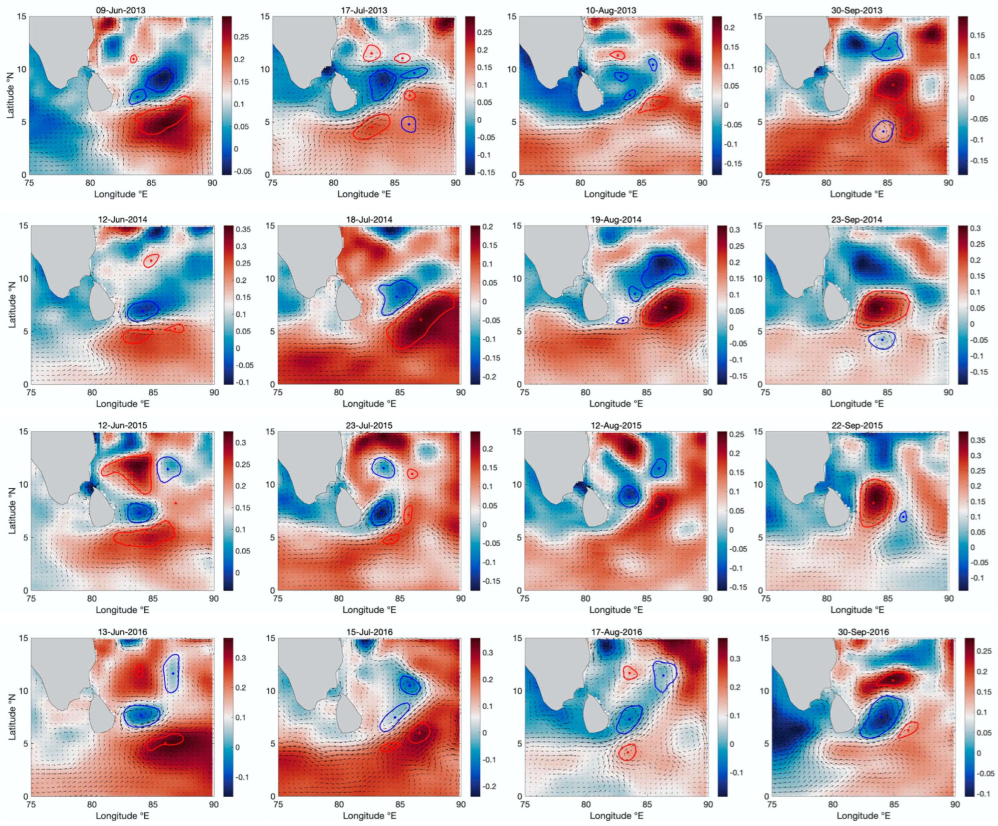
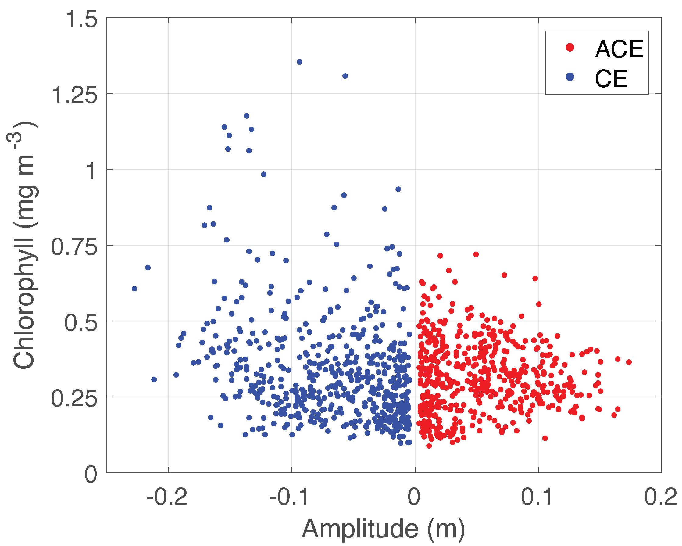
3.4. Eddy Distribution

The eddy distribution and its effect on the chlorophyll in the BoB was studied by ref. [50]. Here, we census eddies near the region of SLD from the Mesoscale Eddy Trajectory Atlas product. The snapshots of all eddies with a lifetime greater than 8 days were censused in the southwestern BoB during the SW monsoon. The SLD box is a hotspot of eddy activities comparing surrounding areas. The majority of cyclonic eddies (CE) occur in the northwest of the SLD box (Figure 8a), while anticyclonic eddies (ACE) are in the southeast (Figure 8b). The area with higher CE activities is consistent with the negative SSHA (Figure 4b) and the dome tracing result of ref. [46]. Usually, upwelling and dowelling happen in the center of a cyclonic and anticyclonic eddy, respectively [51], associating with negative SSHA in CE and positive in ACE. However, the high chlorophyll patch matches better with the region that has higher frequency of ACEs.
Snapshot of eddies and SSHA during the period of SW monsoon show the dipole (a pair of ACE and CE) pattern in this region (Figure 9). The eddy pair is divided by the SMC which intensify in June, mature and move northward in July–August, and decay at the end of September as shown by the surface geostrophic current (Figure 9). A CE and an ACE usually occur on the northwestern and southeastern sides of the SMC, respectively. The core of SLD can be represented by the CE, which moves northward gradually from June to September. This process is more clearly shown in the summer of 2014. At the end of September, an ACE usually covers the region near the east coast of Sri Lanka and the SLD is dismissed. It also shows clear interannual variation, such as the ACE was not shown off the east coast of Sri Lanka at the end of September 2016.

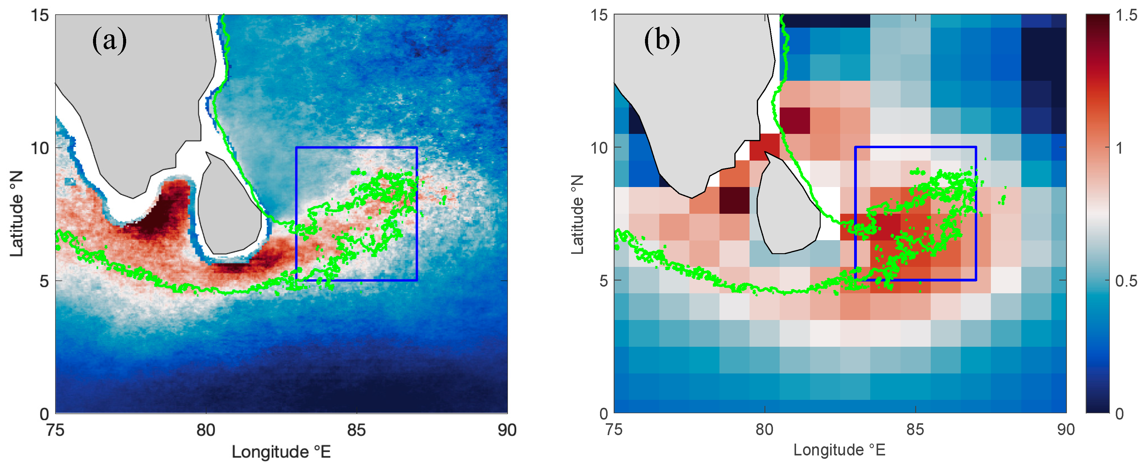
3.5. Frontal Probability

The FP during the SW monsoon is high around the coast of south India and Sri Lanka (Figure 10b), which matches well with the region of high chlorophyll (Figure 2b). The high FP region in the southeast coast of Sri Lanka extends to the SLD, following the pathway of SMC. During the northeast monsoon, the region with high FP near the coast is much smaller (Figure 10a). It shows relatively high FP on the pathway of the East India Coastal Current off the east coast of India and Sri Lanka as shown by the geostrophic current [23]. In the SLD, the FP during winter is also much lower than that of summer.

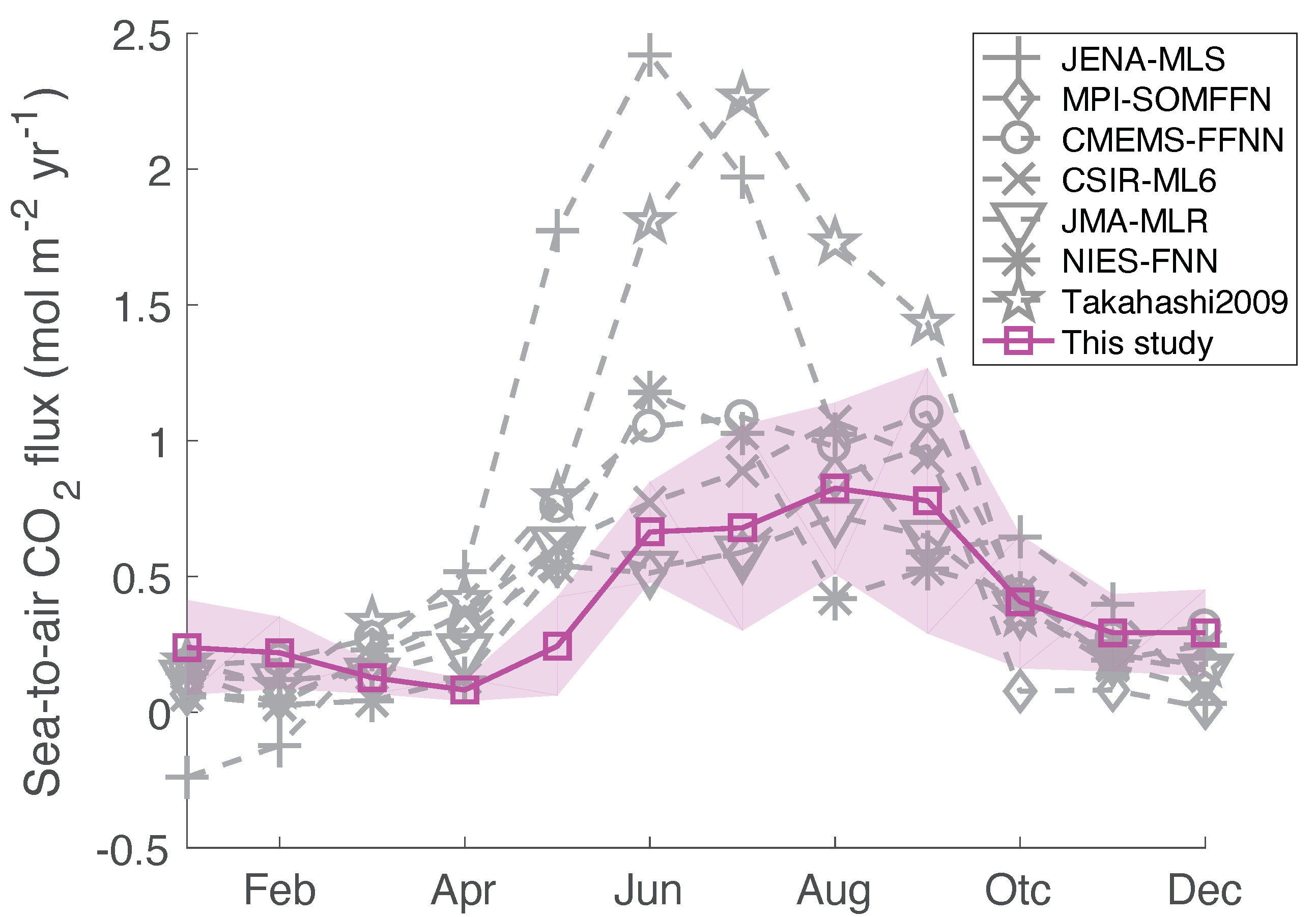
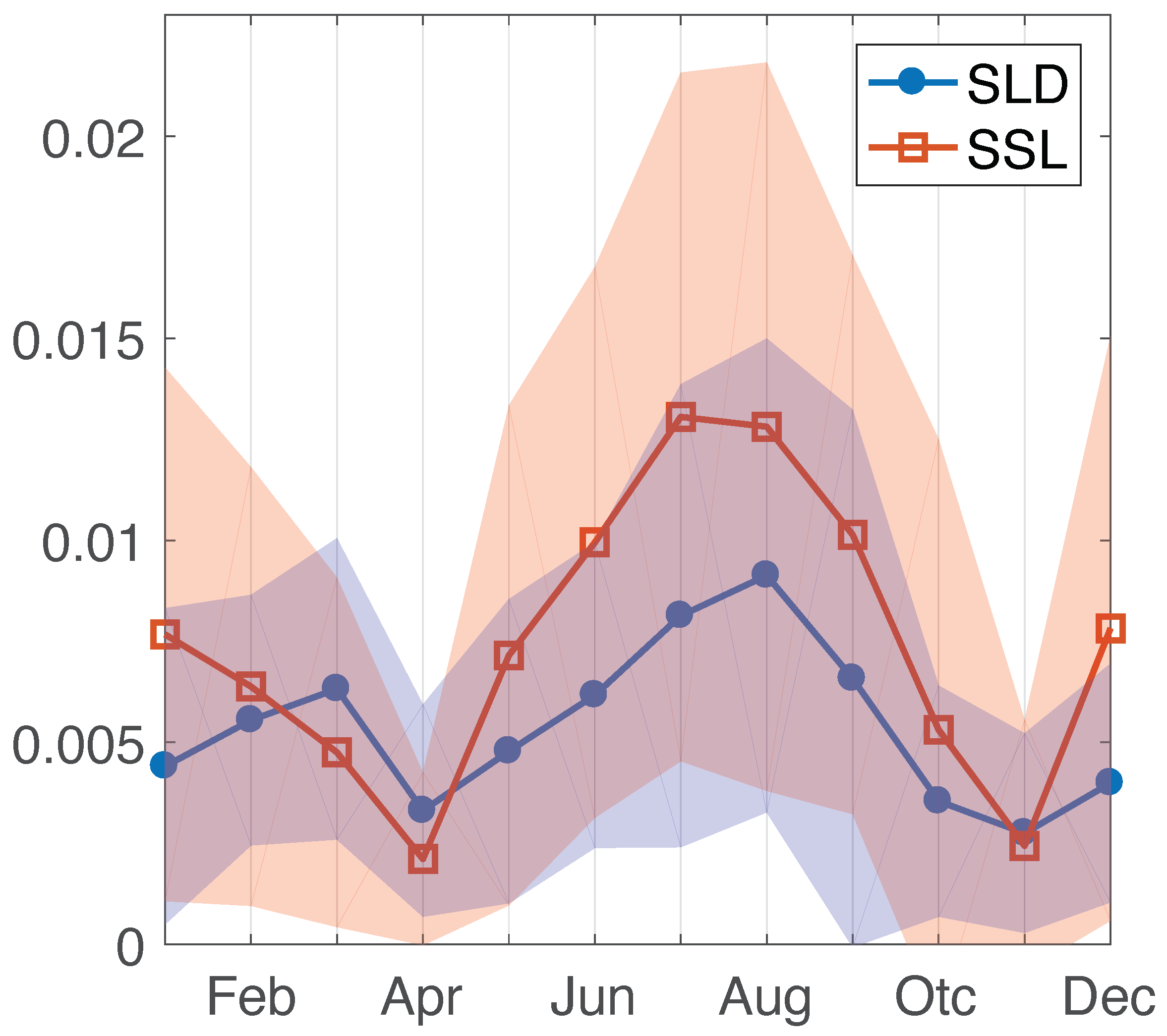
3.6. Sea-to-Air CO2 Flux

The remote sensing of sea-to-air CO2 flux is positive in the SLD box during the SW monsoon (Figure 11a), implying a net carbon source. The high flux region corresponds to the high chlorophyll patch and is consistent with the observation-based SeaFlux dataset by Fay et al. [52] (Figure 11b). The SeaFlux is an ensembled dataset that includes six global observation-based seawater pCO2 mapping products and three wind products with a horizontal resolution of one degree [52]. The algorithm of SeaFlux contains three artificial neural-network-derived products (CMEMS-FFNN, MPI-SOMFFN, NIES-FNN), a mixed layer scheme product (JENA-MLS), a multiple linear regression (JMA-MLR), and a machine learning ensemble (CSIR-ML6) [52]. Our data has a higher spatial resolution than the SeaFlux dataset. Timeseries results also show that the seasonal variability of sea-to-air CO2 flux calculated in this study is consistent with most of the ensemble members of the SeaFlux dataset and the shipboard observation data by Takahashi, et al. [53] (Figure 12). The sea-to-air CO2 fluxes of the SLD region are persistently positive all year round with a maximum (0.82 mol m−2 yr−1) in August. Among these products, JENA-MLS [52] and Takahashi2009 [53] show the strongest outgassing of CO2 during the SW monsoon with ~100% higher flux than the other algorithms.

4. Discussion

4.1. Lateral Advection from the SSL to the SLD

The regional dynamics of the chlorophyll in the SLD region were largely attributed to the positive local wind stress curl which generate upwelling and doming of the nutricline during the SW monsoon [24]. However, the correlation between chlorophyll and wind stress curl is relatively weak, with a R value of 0.35. On the contrary, the R value is 0.65 in the SSL box. Moreover, the chlorophyll in the SLD box has a one-month lag relative to the one in the SSL box (Figure 2a). It was proposed that chlorophyll and/or nutrients are advected from the SSL to the SLD region [3,24]. Similar offshore transport was also found in the South China Sea [54,55] and western Arabian Sea [41] upwelling systems. The concept of delayed island mass effect was recently proposed to describe how nutrients from upwelled water near islands are advected and trigger remote blooms in the open ocean [56].
To test this hypothesis, we applied the forward Lagrangian particle tracking method, which was used in the South China Sea [40]. Each day, 1000 particles were released uniformly in surface waters within the SSL box from 1 to 30 July 2016. The position of every particle was tracked for 30 days unless it hit the boundary of the BoB (75°E in the west and 0°N in the south). Most particles move eastward and are distributed in the entire southwestern BoB in 30 days (Figure 13a). Near the equator, a small fraction of particles moves westward to the Arabian Sea. We censused the fraction of particles that enter the SLD box during the tracking period. In total, >80% of the total released particles entered this region, especially during 10–25 July (Figure 13d). On average, most particles entered the SLD box in the first 10 days (Figure 13b) and left the box 15–30 days after releasing (Figure 13c). Therefore, they stay in the SLD box for about 10–20 days. The tracking result explains the one-month lag of chlorophyll in the SLD box by indicating that chlorophyll and, more likely, nutrients remain in the SLD box for 10–20 days after being advected laterally from the SSL box. If high-nutrient water is transported from the coastal upwelling region to the open ocean via the SMC, it needs additional time delay (3–5 days) for chlorophyll in response to the supply of nutrients, as was noted by refs. [57,58]. However, the high chlorophyll patch does not occur as wide as the region with particles being distributed. It requires nutrients to be consumed out in the SLD box. The tracking result support that the mechanism of delayed island mass effect [56] works in this region.

4.2. Impact of Sea Surface Height, Eddy, and Front on the Chlorophyll

The variability of SSHA in the SLD box shows a higher frequency than that of chlorophyll (Figure 5). EOF analysis reveals that the peak of the PC1 occurs in July (Figure 7), corresponding to the wind stress curl. This probably reflects the local forcing of the monsoon. The timeseries of the PC2 also shows one peak each year, but leads the wind stress curl for 2 months. We interpret this as the mode of inter-monsoon which occurs in May and November. Both PC3 and PC4 show a dipole pattern with intra-seasonal variability (Figure 6 and Figure 7), probably reflecting the westward-propagated eddy activities [59]. The monthly mean SSHA data limit is used to discuss the intra-seasonal variability in detail. However, it was already found that the cycle of SSHA in this region has the cyclicity of 30−60 days [60]. The reflection of equatorial Kelvin waves from the eastern boundary of the Indian Ocean produces a sequence of cyclonic and anticyclonic eddies passed through the box of SLD [23,60]. Therefore, the intra-seasonal variability of SSHA in the SLD region is mainly determined by the far-field oceanic forcing, rather than the local wind forcing. Furthermore, the dipole distribution of CE and ACE (Figure 6 and Figure 7) reflects the westward propagation of upwelling and downwelling Rossby waves. A similar eddy dipole also occurred in the summer upwelling near the coast of Vietnam and the western Arabian Sea [61,62]. However, a recent observation and modeling study suggested that the ACE–CE dipole is generated by topographically trapped Rossby waves near the Sri Lankan coast [63], but both hypotheses emphasized the interaction between oceanic waves and the SMC [63,64]. The region with co-occurrence of frequent ACE and high chlorophyll patch may imply the contribution of ACEs. We analyzed the mean chlorophyll concentration inside each eddy that occurred in the SLD box during the SW monsoon (Figure 14). The chlorophyll extremes (>0.75 mg m−3) in the CE are higher than that in ACE, implying that the CE-induced upwelling would increase the chlorophyll concentration. However, the mean concentration of all CEs (0.34 mg m−3) does not have a significant difference from that of all ACEs (0.34 mg m−3). Therefore, the occurrence of ACE in the high-chlorophyll patch has a neglected or weak-negative impact on the chlorophyll.
Both the BoBBLE observation and modeling results showed that the SLD region develops prominent deep chlorophyll maxima (DCM) at intermediate depths (20–50 m) [30]. The DCM is stronger in the region of the SLD and the SMC due to the corresponding Ekman pumping [30], but weaker outside the dome. Therefore, another possibility is that the effect of CE increases the concentration of DCM that is not observed by satellite. However, the model result showed that the SMC region features the strongest DCM as well as the highest depth-integrated chlorophyll [30]. Thus, the change in surface chlorophyll observed by satellite can represent the subsurface condition. We suggest eddy activities have limited direct influence on the distribution of chlorophyll in the SLD box.
In the coastal upwelling system, FP is an effective indicator of hydrodynamics [39,41,65]. When the along-shore wind forces off-shore Ekman transport, cold water from the subsurface is forced to upwell to the surface and fronts subsequently develop around the boundary of water masses, associating with a strong SST gradient [17,66]. The cold water near the coast further reduces the wind aloft and produces a positive wind stress curl [67,68,69]. Both the wind stress curl and FP in the SSL box show the same seasonality and are highly correlated with chlorophyll (Figure 3b and Figure 15). The peak of FP in winter can interpret the winter chlorophyll maximum in the SSL. The wind stress curl, however, does not have the winter maximum (Figure 3b). FP also reveals the sub-mesoscale process, which produces strong vertical mixing/convection and provides nutrients to the surface layer [66,70,71]. In the SLD box, the maxima of FP occur in August, the same month as the occurrence of chlorophyll maximum. In terms of the spatial distribution, the high FP occurs on the pathway of SMC (Figure 10b). The Arabian Sea high-salinity water enters the southern BoB with the SMC [72]. It is proposed that the advection of high-salinity water decreases stratification [25]. CE in the northwest side can upwell the high-salinity water from the subsurface to the surface. Therefore, the interaction between the SMC and mesoscale eddies can produce fronts and strong mixing along the SMC [63,73,74]. The current and surface wind are oriented in the same direction, which may also trigger instabilities and sub-mesoscale fronts [75]. In addition, the region of SLD usually receives less precipitation during the SW monsoon [76,77], but some extreme precipitation events can result in frontal filament and strong sub-mesoscale mixing in this region [78]. The match of phases between FP and chlorophyll in the SLD implies that the front-related sub-mesoscale mixing contributes to the increase of chlorophyll.

4.3. Dynamics of the Air–Sea CO2 Flux

It is well known that the permeant upwelling systems such as the Humboldt upwelling in the East Pacific and equatorial upwelling in the eastern equatorial Pacific are significant sources of atmospheric CO2 [79,80,81]. However, the physical and biological control of seawater pCO2 in the southwestern BoB is not well understood. The first-order mechanism of the SLD is wind-induced Ekman pumping rather than the Ekman transport in the coastal upwelling system. Most biogeochemical models reproduced a weak source or even a sink during the SW monsoon in the SLD [26,82]. However, the observational CO2 flux during the SW monsoon period reveals that it is a moderate–strong source of CO2 with a flux of 1.79 mol m−2 yr−1 [53]. The bias of models is due to overestimated primary productivity [82]. Our calculated air–sea CO2 flux based on remote sensing products has higher temporal and spatial resolution than the shipboard observations. The seasonal variability in CO2 flux is consistent with the result of Takahashi et al. (2009), but has a smaller amplitude (Figure 12). Because of the scarcity of observation data, the flux must be validated further in future studies. Recent observation results from BoBBLE showed that the upwelled subsurface water from SMC has a higher dissolved inorganic carbon (DIC)-to-nitrate ratio than the conventional Redfield ratio (106:16) [25]. It is assumed that the upwelled nutrient is consumed by phytoplankton because the nitrate concentration is extremely low in this region. The excess of DIC can act as the source to the atmosphere [25]. As discussed above, the high wind stress curl and FP occurred on the pathway of SMC, suggesting the strongest upwelling and/or sub-mesoscale process in this region. The highest CO2 flux also matches the pathway of SMC (Figure 11a). Our results support that the advection of high-salinity water via the SMC decreases stratification, combining with the frontal process to favor deeper mixing and ventilation in the SLD during SW monsoon.

5. Conclusions

In this paper, we studied the controlling factors for the formation of the SLD during the SW monsoon. The positive wind stress curl is the first-order forcing. The plateau of the positive wind stress curl was quickly established from May, which interprets the onset of increasing in chlorophyll. There is a one-month lag of chlorophyll in the SLD region relative to the SSL region, indicating the role of the lateral advection of nutrients from coastal upwelling waters of SSL via the SMC.
Cyclonic eddies introduce a limited increase of chlorophyll in the SLD. The more frequent occurrence of anticyclonic eddies in the high-chlorophyll patch indicates that eddy activities have a weak impact on the chlorophyll variability.
Higher FP in the SLD region corresponds to the SMC, implying the occurrence of fronts and strong mixing on the pathway of SMC.
The subsurface water of the SLD has a higher DIC-to-nutrients ratio than the conventional Redfield ratio. The wind-driven upwelling and/or sub-mesoscale process make the surface waters have excess DIC and, hence, establish them as a carbon source to the atmosphere.

Supplementary Materials

The following supporting information can be downloaded at: https://www.mdpi.com/article/10.3390/rs14143239/s1, Figure S1: Seawater pCO2 observation data used for training in the Indian Ocean; Figure S2: Wind stress curl of ERA5 vs. CCMP wind product; Figure S3: Timeseries of mean SSHA in the SLD region from 1998 to 2020.

Author Contributions

Conceptualization: W.M.; methodology: W.M., Y.W., Y.B., Y.Y., Z.Z. and J.X.; writing—original draft preparation: W.M.; writing—review and editing: Y.W., Y.B. and Y.Y.; visualization: W.M. and X.M.; funding acquisition: W.M. All authors have read and agreed to the published version of the manuscript.

Funding

This research was funded by the Strategic Priority Research Program, Chinese Academy of Sciences, China, Grant No. XDB42000000; Global Change and Air–Sea Interaction Program Phase II (“Joint Advanced Marine and Ecological Studies in the Bay of Bengal and the Eastern Equatorial Indian Ocean (JAMES)”, Grant No. GASI-01-EIND-STwin); the National Natural Science Foundation of China, Grant No. 41876123; SOED research program, Grant No. SOEDZZ2104.

Data Availability Statement

Monthly and 5-day gridded data of the Ocean Colour Climate Change Initiative (Ocean Color CCI) v5.0 are available from the ESA database (https://www.oceancolour.org/thredds/catalog-cci.html, accessed on 30 January 2022). Daily and monthly sea surface height anomaly (SSHA) and surface geostrophic current data are available from the E.U. Copernicus Marine Service (https://resources.marine.copernicus.eu/product-detail/SEALEVEL_GLO_PHY_L4_MY_008_047/INFORMATION, accessed on 30 January 2022). Mesoscale Eddy Trajectory Atlas products (META3.1exp DT) are available from AVISO+ (https://data.aviso.altimetry.fr/aviso-gateway/data/META3.1exp_DT/META3.1exp_DT_allsat/, accessed on 30 January 2022). ERA5 reanalysis products are available from the Climate Data Store of E.U. Copernicus (https://cds.climate.copernicus.eu/cdsapp#!/dataset/reanalysis-era5-single-levels?tab=overview, accessed on 30 January 2022). MODIS SST data are available from the NASA database (http://oceandata.sci.gsfc.nasa.gov/directaccess/MODIS-Aqua/Mapped/Daily/4km/sst4/, accessed on 30 January 2022). HYCOM reanalysis product of expt_57.2 is available from its website (https://tds.hycom.org/thredds/catalogs/GLBv0.08/expt_57.2.html, accessed on 10 February 2022). Variables in Table 1 are available as follows: Wind speed (https://resources.marine.copernicus.eu/product-detail/WIND_GLO_WIND_L4_REP_OBSERVATIONS_012_006/INFORMATION, accessed on 30 January 2022); SST (https://www.ncei.noaa.gov/products/optimum-interpolation-sst, accessed on 30 January 2022); SSS and MLD (https://resources.marine.copernicus.eu/product-detail/GLOBAL_REANALYSIS_PHY_001_031/INFORMATION, accessed on 30 January 2022); CarbonTracker CT2019B (https://gml.noaa.gov/ccgg/carbontracker/, accessed on 30 January 2022).

Acknowledgments

We thank Siqi Zhang for helping to prepare the CO2 flux data for the BoB. The open-source Climate Data Toolbox for MATLAB [83] helped us to implement data analysis. We are grateful to the academic editor and reviewers for constructive suggestions.

Conflicts of Interest

The authors declare no conflict of interest.

Abbreviations

ACEAnticyclonic eddy
BoBBay of Bengal
BoBBLEBay of Bengal Boundary Layer Experiment
CECyclonic eddy
DCMDeep chlorophyll maxima
NPPNet primary productivity
MLDMixed layer depth
Ocean Color CCIOcean Colour Climate Change Initiative
RrsRemote-sensing reflectance
SCSSouth China Sea
SLDSri Lanka dome
SMCSouthwest monsoon current
SSHASea surface height anomaly
SSSSea surface salinity
SSTSea surface temperature

References

  1. Schott, F.A.; McCreary, J.P. The monsoon circulation of the Indian Ocean. Prog. Oceanogr. 2001, 51, 1–123. [Google Scholar] [CrossRef]
  2. Thapliyal, V.; Rajeevan, M. MONSOON|Prediction. In Encyclopedia of Atmospheric Sciences; Holton, J.R., Ed.; Academic Press: Oxford, UK, 2003; pp. 1391–1400. [Google Scholar] [CrossRef]
  3. Vinayachandran, P.N.M.; Masumoto, Y.; Roberts, M.J.; Huggett, J.A.; Halo, I.; Chatterjee, A.; Amol, P.; Gupta, G.V.M.; Singh, A.; Mukherjee, A.; et al. Reviews and syntheses: Physical and biogeochemical processes associated with upwelling in the Indian Ocean. Biogeosciences 2021, 18, 5967–6029. [Google Scholar] [CrossRef]
  4. Li, Y.; Qiu, Y.; Hu, J.; Aung, C.; Lin, X.; Dong, Y. Springtime Upwelling and Its Formation Mechanism in Coastal Waters of Manaung Island, Myanmar. Remote Sens. 2020, 12, 3777. [Google Scholar] [CrossRef]
  5. Vic, C.; Capet, X.; Roullet, G.; Carton, X. Western boundary upwelling dynamics off Oman. Ocean. Dyn. 2017, 67, 585–595. [Google Scholar] [CrossRef] [Green Version]
  6. Elliott, A.J.; Savidge, G. Some features of the upwelling off Oman. J. Mar. Res. 1990, 48, 319–333. [Google Scholar] [CrossRef]
  7. Lighthill, M.J. Dynamic response of the Indian Ocean to onset of the Southwest Monsoon. Philos. Trans. R. Soc. London. Ser. A Math. Phys. Sci. 1969, 265, 45–92. [Google Scholar] [CrossRef]
  8. Chatterjee, A.; Kumar, B.P.; Prakash, S.; Singh, P. Annihilation of the Somali upwelling system during summer monsoon. Sci. Rep. 2019, 9, 7598. [Google Scholar] [CrossRef]
  9. McCreary, J.P.; Kundu, P.K.; Molinari, R.L. A numerical investigation of dynamics, thermodynamics and mixed-layer processes in the Indian Ocean. Prog. Oceanogr. 1993, 31, 181–244. [Google Scholar] [CrossRef]
  10. Shah, P.; Sajeev, R.; Gopika, N. Study of Upwelling along the West Coast of India—A Climatological Approach. J. Coast. Res. 2015, 31, 1151–1158. [Google Scholar] [CrossRef]
  11. Rao, A.D.; Joshi, M.; Ravichandran, M. Oceanic upwelling and downwelling processes in waters off the west coast of India. Ocean. Dyn. 2008, 58, 213–226. [Google Scholar] [CrossRef]
  12. Xu, T.; Wei, Z.; Li, S.; Susanto, R.D.; Radiarta, N.; Yuan, C.; Setiawan, A.; Kuswardani, A.; Agustiadi, T.; Trenggono, M. Satellite-Observed Multi-Scale Variability of Sea Surface Chlorophyll-a Concentration along the South Coast of the Sumatra-Java Islands. Remote Sens. 2021, 13, 2817. [Google Scholar] [CrossRef]
  13. Susanto, R.D.; Gordon, A.L.; Zheng, Q. Upwelling along the coasts of Java and Sumatra and its relation to ENSO. Geophys. Res. Lett. 2001, 28, 1599–1602. [Google Scholar] [CrossRef]
  14. Narvekar, J.; Roy Chowdhury, R.; Gaonkar, D.; Kumar, P.K.D.; Prasanna Kumar, S. Observational evidence of stratification control of upwelling and pelagic fishery in the eastern Arabian Sea. Sci. Rep. 2021, 11, 7293. [Google Scholar] [CrossRef] [PubMed]
  15. Madhupratap, M.; Nair, K.N.V.; Gopalakrishnan, T.C.; Haridas, P.; Nair, K.K.C.; Venugopal, P.; Gauns, M. Arabian Sea oceanography and fisheries of the west coast of India. Curr. Sci. 2001, 81, 355–361. [Google Scholar]
  16. Vinayachandran, P.N.; Yamagata, T. Monsoon Response of the Sea around Sri Lanka: Generation of Thermal Domesand Anticyclonic Vortices. J. Phys. Oceanogr. 1998, 28, 1946–1960. [Google Scholar] [CrossRef]
  17. De Vos, A.; Pattiaratchi, C.B.; Wijeratne, E.M.S. Surface circulation and upwelling patterns around Sri Lanka. Biogeosciences 2014, 11, 5909–5930. [Google Scholar] [CrossRef] [Green Version]
  18. Burns, J.M.; Subrahmanyam, B.; Murty, V.S.N. On the dynamics of the Sri Lanka Dome in the Bay of Bengal. J. Geophys. Res. Oceans 2017, 122, 7737–7750. [Google Scholar] [CrossRef]
  19. Vinayachandran, P.N.; Masumoto, Y.; Mikawa, T.; Yamagata, T. Intrusion of the Southwest Monsoon Current into the Bay of Bengal. J. Geophys. Res. Oceans 1999, 104, 11077–11085. [Google Scholar] [CrossRef]
  20. Su, D.; Wijeratne, S.; Pattiaratchi, C.B. Monsoon Influence on the Island Mass Effect around the Maldives and Sri Lanka. Front. Mar. Sci. 2021, 8, 645672. [Google Scholar] [CrossRef]
  21. Doty, M.S.; Oguri, M. The Island Mass Effect. ICES J. Mar. Sci. 1956, 22, 33–37. [Google Scholar] [CrossRef]
  22. Pramanik, S.; Sil, S.; Gangopadhyay, A.; Singh, M.K.; Behera, N. Interannual variability of the Chlorophyll-a concentration over Sri Lankan Dome in the Bay of Bengal. Int. J. Remote Sens. 2020, 41, 5974–5991. [Google Scholar] [CrossRef]
  23. Phillips, H.E.; Tandon, A.; Furue, R.; Hood, R.; Ummenhofer, C.C.; Benthuysen, J.A.; Menezes, V.; Hu, S.; Webber, B.; Sanchez-Franks, A.; et al. Progress in understanding of Indian Ocean circulation, variability, air-sea exchange, and impacts on biogeochemistry. Ocean Sci. 2021, 17, 1677–1751. [Google Scholar] [CrossRef]
  24. Vinayachandran, P.N.; Chauhan, P.; Mohan, M.; Nayak, S. Biological response of the sea around Sri Lanka to summer monsoon. Geophys. Res. Lett. 2004, 31. [Google Scholar] [CrossRef]
  25. Roy, R.; Vinayachandran, P.N.; Sarkar, A.; George, J.; Parida, C.; Lotliker, A.; Prakash, S.; Choudhury, S.B. Southern Bay of Bengal: A possible hotspot for CO2 emission during the summer monsoon. Prog. Oceanogr. 2021, 197, 102638. [Google Scholar] [CrossRef]
  26. Chakraborty, K.; Valsala, V.; Gupta, G.V.M.; Sarma, V.V.S.S. Dominant Biological Control over Upwelling on pCO2 in Sea East of Sri Lanka. J. Geophys. Res. Biogeosci. 2018, 123, 3250–3261. [Google Scholar] [CrossRef]
  27. Lévy, M.; Shankar, D.; André, J.M.; Shenoi, S.S.C.; Durand, F.; de Boyer Montégut, C. Basin-wide seasonal evolution of the Indian Ocean’s phytoplankton blooms. J. Geophys. Res. Ocean. 2007, 112. [Google Scholar] [CrossRef] [Green Version]
  28. Yuan, X.; Salama, M.S.; Su, Z. An Observational Perspective of Sea Surface Salinity in the Southwestern Indian Ocean and Its Role in the South Asia Summer Monsoon. Remote Sens. 2018, 10, 1930. [Google Scholar] [CrossRef] [Green Version]
  29. Vinayachandran, P.N.; Matthews, A.J.; Kumar, K.V.; Sanchez-Franks, A.; Thushara, V.; George, J.; Vijith, V.; Webber, B.G.M.; Queste, B.Y.; Roy, R.; et al. BoBBLE: Ocean–Atmosphere Interaction and Its Impact on the South Asian Monsoon. Bull. Am. Meteorol. Soc. 2018, 99, 1569–1587. [Google Scholar] [CrossRef] [Green Version]
  30. Thushara, V.; Vinayachandran, P.N.M.; Matthews, A.J.; Webber, B.G.M.; Queste, B.Y. Vertical distribution of chlorophyll in dynamically distinct regions of the southern Bay of Bengal. Biogeosciences 2019, 16, 1447–1468. [Google Scholar] [CrossRef] [Green Version]
  31. Xu, Y.; Wu, Y.; Wang, H.; Zhang, Z.; Li, J.; Zhang, J. Seasonal and interannual variabilities of chlorophyll across the eastern equatorial Indian Ocean and Bay of Bengal. Prog. Oceanogr. 2021, 198, 102661. [Google Scholar] [CrossRef]
  32. Sharada, M.K.; Swathi, P.S.; Yajnik, K.S.; Kalyani Devasena, C. Role of biology in the air-sea carbon flux in the Bay of Bengal and Arabian Sea. J. Earth Syst. Sci. 2008, 117, 429–447. [Google Scholar] [CrossRef] [Green Version]
  33. Laruelle, G.G.; Lauerwald, R.; Pfeil, B.; Regnier, P. Regionalized global budget of the CO2 exchange at the air-water interface in continental shelf seas. Glob. Biogeochem. Cycles 2014, 28, 1199–1214. [Google Scholar] [CrossRef]
  34. Bai, Y.; Cai, W.-J.; He, X.; Zhai, W.; Pan, D.; Dai, M.; Yu, P. A mechanistic semi-analytical method for remotely sensing sea surface pCO2 in river-dominated coastal oceans: A case study from the East China Sea. J. Geophys. Res. Oceans 2015, 120, 2331–2349. [Google Scholar] [CrossRef]
  35. Chen, S.; Sutton, A.J.; Hu, C.; Chai, F. Quantifying the Atmospheric CO2 Forcing Effect on Surface Ocean pCO2 in the North Pacific Subtropical Gyre in the Past Two Decades. Front. Mar. Sci. 2021, 8, 636881. [Google Scholar] [CrossRef]
  36. Le, C.; Gao, Y.; Cai, W.-J.; Lehrter, J.C.; Bai, Y.; Jiang, Z.-P. Estimating summer sea surface pCO2 on a river-dominated continental shelf using a satellite-based semi-mechanistic model. Remote Sens. Environ. 2019, 225, 115–126. [Google Scholar] [CrossRef]
  37. Parard, G.; Charantonis, A.A.; Rutgerson, A. Remote sensing the sea surface CO2 of the Baltic Sea using the SOMLO methodology. Biogeosciences 2015, 12, 3369–3384. [Google Scholar] [CrossRef] [Green Version]
  38. Sathyendranath, S.; Brewin, R.J.W.; Brockmann, C.; Brotas, V.; Calton, B.; Chuprin, A.; Cipollini, P.; Couto, A.B.; Dingle, J.; Doerffer, R.; et al. An Ocean-Colour Time Series for Use in Climate Studies: The Experience of the Ocean-Colour Climate Change Initiative (OC-CCI). Sensors 2019, 19, 4285. [Google Scholar] [CrossRef] [Green Version]
  39. Wang, Y.; Castelao, R.M.; Yuan, Y. Seasonal variability of alongshore winds and sea surface temperature fronts in Eastern Boundary Current Systems. J. Geophys. Res. Oceans 2015, 120, 2385–2400. [Google Scholar] [CrossRef]
  40. Ma, W.; Xiu, P.; Chai, F.; Ran, L.; Wiesner, M.G.; Xi, J.; Yan, Y.; Fredj, E. Impact of mesoscale eddies on the source funnel of sediment trap measurements in the South China Sea. Prog. Oceanogr. 2021, 194, 102566. [Google Scholar] [CrossRef]
  41. Wang, Y.; Ma, W.; Zhou, F.; Chai, F. Frontal variability and its impact on chlorophyll in the Arabian Sea. J. Mar. Syst. 2021, 218, 103545. [Google Scholar] [CrossRef]
  42. Grinsted, A.; Moore, J.C.; Jevrejeva, S. Application of the cross wavelet transform and wavelet coherence to geophysical time series. Nonlinear Processes Geophys. 2004, 11, 561–566. [Google Scholar] [CrossRef]
  43. Bakker, D.C.E.; Pfeil, B.; Landa, C.S.; Metzl, N.; O’Brien, K.M.; Olsen, A.; Smith, K.; Cosca, C.; Harasawa, S.; Jones, S.D.; et al. A multi-decade record of high-quality fCO2 data in version 3 of the Surface Ocean CO2 Atlas (SOCAT). Earth Syst. Sci. Data 2016, 8, 383–413. [Google Scholar] [CrossRef] [Green Version]
  44. Kraus, E.B.; Businger, J.A. Atmosphere-Ocean Interaction; Oxford University Press: Oxford, UK, 1994. [Google Scholar]
  45. Mears, C.A.; Scott, J.; Wentz, F.J.; Ricciardulli, L.; Leidner, S.M.; Hoffman, R.; Atlas, R. A Near-Real-Time Version of the Cross-Calibrated Multiplatform (CCMP) Ocean Surface Wind Velocity Data Set. J. Geophys. Res. Oceans 2019, 124, 6997–7010. [Google Scholar] [CrossRef]
  46. Cullen, K.E.; Shroyer, E.L. Seasonality and interannual variability of the Sri Lanka dome. Deep. Sea Res. Part II Top. Stud. Oceanogr. 2019, 168, 104642. [Google Scholar] [CrossRef]
  47. Chen, Y.; Shi, H.; Zhao, H. Summer Phytoplankton Blooms Induced by Upwelling in the Western South China Sea. Front. Mar. Sci. 2021, 8, 740130. [Google Scholar] [CrossRef]
  48. Narayanan Nampoothiri, S.V.; Ramu, C.V.; Rasheed, K.; Sarma, Y.V.B.; Gupta, G.V.M. Observational evidence on the coastal upwelling along the northwest coast of India during summer monsoon. Environ. Monit. Assess. 2021, 194, 5. [Google Scholar] [CrossRef]
  49. Narayanan Nampoothiri, S.V.; Sachin, T.S.; Rasheed, K. Dynamics and forcing mechanisms of upwelling along the south eastern Arabian sea during south west monsoon. Reg. Stud. Mar. Sci. 2020, 40, 101519. [Google Scholar] [CrossRef]
  50. Yang, X.; Xu, G.; Liu, Y.; Sun, W.; Xia, C.; Dong, C. Multi-Source Data Analysis of Mesoscale Eddies and Their Effects on Surface Chlorophyll in the Bay of Bengal. Remote Sens. 2020, 12, 3485. [Google Scholar] [CrossRef]
  51. Gaube, P.; McGillicuddy, D.J., Jr.; Chelton, D.B.; Behrenfeld, M.J.; Strutton, P.G. Regional variations in the influence of mesoscale eddies on near-surface chlorophyll. J. Geophys. Res. Oceans 2014, 119, 8195–8220. [Google Scholar] [CrossRef] [Green Version]
  52. Fay, A.R.; Gregor, L.; Landschützer, P.; McKinley, G.A.; Gruber, N.; Gehlen, M.; Iida, Y.; Laruelle, G.G.; Rödenbeck, C.; Roobaert, A.; et al. SeaFlux: Harmonization of air-sea CO2 fluxes from surface pCO2 data products using a standardized approach. Earth Syst. Sci. Data 2021, 13, 4693–4710. [Google Scholar] [CrossRef]
  53. Takahashi, T.; Sutherland, S.C.; Wanninkhof, R.; Sweeney, C.; Feely, R.A.; Chipman, D.W.; Hales, B.; Friederich, G.; Chavez, F.; Sabine, C.; et al. Climatological mean and decadal change in surface ocean pCO2, and net sea-air CO2 flux over the global oceans. Deep. Sea Res. Part II Top. Stud. Oceanogr. 2009, 56, 554–577. [Google Scholar] [CrossRef]
  54. Lu, W.; Oey, L.Y.; Liao, E.; Zhuang, W.; Yan, X.H.; Jiang, Y. Physical modulation to the biological productivity in the summer Vietnam upwelling system. Ocean Sci. 2018, 14, 1303–1320. [Google Scholar] [CrossRef] [Green Version]
  55. Liang, W.; Tang, D.; Luo, X. Phytoplankton size structure in the western South China Sea under the influence of a ‘jet-eddy system’. J. Mar. Syst. 2018, 187, 82–95. [Google Scholar] [CrossRef]
  56. Messié, M.; Petrenko, A.; Doglioli, A.M.; Aldebert, C.; Martinez, E.; Koenig, G.; Bonnet, S.; Moutin, T. The Delayed Island Mass Effect: How Islands can Remotely Trigger Blooms in the Oligotrophic Ocean. Geophys. Res. Lett. 2020, 47, e2019GL085282. [Google Scholar] [CrossRef] [Green Version]
  57. Trombetta, T.; Vidussi, F.; Mas, S.; Parin, D.; Simier, M.; Mostajir, B. Water temperature drives phytoplankton blooms in coastal waters. PLoS ONE 2019, 14, e0214933. [Google Scholar] [CrossRef] [PubMed] [Green Version]
  58. Van Oostende, N.; Dunne, J.P.; Fawcett, S.E.; Ward, B.B. Phytoplankton succession explains size-partitioning of new production following upwelling-induced blooms. J. Mar. Syst. 2015, 148, 14–25. [Google Scholar] [CrossRef]
  59. Huang, H.; Wang, D.; Yang, L.; Huang, K. Enhanced Intraseasonal Variability of the Upper Layers in the Southern Bay of Bengal During the Summer 2016. J. Geophys. Res. Oceans 2021, 126, e2021JC017459. [Google Scholar] [CrossRef]
  60. Cheng, X.; McCreary, J.P.; Qiu, B.; Qi, Y.; Du, Y. Intraseasonal-to-semiannual variability of sea-surface height in the astern, equatorial Indian Ocean and southern Bay of Bengal. J. Geophys. Res. Oceans 2017, 122, 4051–4067. [Google Scholar] [CrossRef]
  61. Wang, G.; Chen, D.; Su, J. Generation and life cycle of the dipole in the South China Sea summer circulation. J. Geophys. Res. Oceans 2006, 111, C06002. [Google Scholar] [CrossRef] [Green Version]
  62. Ni, Q.; Zhai, X.; Wang, G.; Hughes, C.W. Widespread Mesoscale Dipoles in the Global Ocean. J. Geophys. Res. Oceans 2020, 125, e2020JC016479. [Google Scholar] [CrossRef]
  63. Pirro, A.; Fernando, H.J.S.; Wijesekera, H.W.; Jensen, T.G.; Centurioni, L.R.; Jinadasa, S.U.P. Eddies and currents in the Bay of Bengal during summer monsoons. Deep. Sea Res. Part II Top. Stud. Oceanogr. 2020, 172, 104728. [Google Scholar] [CrossRef]
  64. Webber, B.G.M.; Matthews, A.J.; Vinayachandran, P.N.; Neema, C.P.; Sanchez-Franks, A.; Vijith, V.; Amol, P.; Baranowski, D.B. The Dynamics of the Southwest Monsoon Current in 2016 from High-Resolution in Situ Observations and Models. J. Phys. Oceanogr. 2018, 48, 2259–2282. [Google Scholar] [CrossRef]
  65. Yu, Y.; Wang, Y.; Cao, L.; Tang, R.; Chai, F. The ocean-atmosphere interaction over a summer upwelling system in the South China Sea. J. Mar. Syst. 2020, 208, 103360. [Google Scholar] [CrossRef]
  66. Jinadasa, S.U.P.; Lozovatsky, I.; Planella-Morató, J.; Nash, J.; MacKinnon, J.; Lucas, A.; Wijesekera, H.; Fernando, H. Ocean Turbulence and Mixing Around Sri Lanka and in Adjacent Waters of the Northern Bay of Bengal. Oceanography 2016, 29, 170–179. [Google Scholar] [CrossRef] [Green Version]
  67. Li, Y.; Qiu, Y.; Hu, J.; Aung, C.; Lin, X.; Jing, C.; Zhang, J. The Strong Upwelling Event off the Southern Coast of Sri Lanka in 2013 and Its Relationship with Indian Ocean Dipole Events. J. Climate 2021, 34, 3555–3569. [Google Scholar] [CrossRef]
  68. Enriquez, A.G.; Friehe, C.A. Effects of Wind Stress and Wind Stress Curl Variability on Coastal Upwelling. J. Phys. Oceanogr. 1995, 25, 1651–1671. [Google Scholar] [CrossRef] [Green Version]
  69. McCreary, J.P.; Murtugudde, R.; Vialard, J.; Vinayachandran, P.N.; Wiggert, J.D.; Hood, R.R.; Shankar, D.; Shetye, S. Biophysical Processes in the Indian Ocean. In Indian Ocean Biogeochemical Processes and Ecological Variability; Geophysical Monograph Series; John Wiley & Sons: Hoboken, NJ, USA, 2009; pp. 9–32. [Google Scholar] [CrossRef] [Green Version]
  70. Zhong, Y.; Bracco, A.; Tian, J.; Dong, J.; Zhao, W.; Zhang, Z. Observed and simulated submesoscale vertical pump of an anticyclonic eddy in the South China Sea. Sci. Rep. 2017, 7, 44011. [Google Scholar] [CrossRef]
  71. Lévy, M.; Franks, P.J.S.; Smith, K.S. The role of submesoscale currents in structuring marine ecosystems. Nat. Commun. 2018, 9, 4758. [Google Scholar] [CrossRef] [Green Version]
  72. Murty, V.S.N.; Sarma, Y.V.B.; Rao, D.P.; Murty, C.S. Water characteristics, mixing and circulation in the Bay of Bengal during southwest monsoon. J. Mar. Res. 1992, 50, 207–228. [Google Scholar] [CrossRef]
  73. Lozovatsky, I.; Pirro, A.; Jarosz, E.; Wijesekera, H.W.; Jinadasa, S.U.P.; Fernando, H.J.S. Turbulence at the periphery of Sri Lanka dome. Deep. Sea Res. Part II Top. Stud. Oceanogr. 2019, 168, 104614. [Google Scholar] [CrossRef]
  74. Sarkar, S.; Pham, H.; Ramachandran, S.; Nash, J.; Tandon, A.; Buckley, J.; Lotliker, A.; Omand, M. The Interplay between Submesoscale Instabilities and Turbulence in the Surface Layer of the Bay of Bengal. Oceanography 2016, 29, 146–157. [Google Scholar] [CrossRef] [Green Version]
  75. Thomas, L.N.; Lee, C.M. Intensification of Ocean Fronts by Down-Front Winds. J. Phys. Oceanogr. 2005, 35, 1086–1102. [Google Scholar] [CrossRef]
  76. Keshtgar, B.; Alizadeh-Choobari, O.; Irannejad, P. Seasonal and interannual variations of the intertropical convergence zone over the Indian Ocean based on an energetic perspective. Clim. Dyn. 2020, 54, 3627–3639. [Google Scholar] [CrossRef]
  77. Das, U.; Vinayachandran, P.N.; Behara, A. Formation of the southern Bay of Bengal cold pool. Clim. Dyn. 2016, 47, 2009–2023. [Google Scholar] [CrossRef]
  78. Pham, H.T.; Sarkar, S. The role of turbulence in strong submesoscale fronts of the Bay of Bengal. Deep. Sea Res. Part II Top. Stud. Oceanogr. 2019, 168, 104644. [Google Scholar] [CrossRef]
  79. Brady, R.X.; Lovenduski, N.S.; Alexander, M.A.; Jacox, M.; Gruber, N. On the role of climate modes in modulating the air–sea CO2 fluxes in eastern boundary upwelling systems. Biogeosciences 2019, 16, 329–346. [Google Scholar] [CrossRef] [Green Version]
  80. Feely, R.A. Seasonal and interannual variability of CO2 in the equatorial Pacific. Deep Sea Res. Part II Top. Stud. Oceanogr. 2002, 49, 2443–2469. [Google Scholar] [CrossRef]
  81. Valsala, V.K.; Roxy, M.K.; Ashok, K.; Murtugudde, R. Spatiotemporal characteristics of seasonal to multidecadal variability of pCO2 and air–sea CO2 fluxes in the equatorial Pacific Ocean. J. Geophys. Res. Oceans 2014, 119, 8987–9012. [Google Scholar] [CrossRef]
  82. Sreeush, M.G.; Valsala, V.; Pentakota, S.; Prasad, K.V.S.R.; Murtugudde, R. Biological production in the Indian Ocean upwelling zones—Part 1: Refined estimation via the use of a variable compensation depth in ocean carbon models. Biogeosciences 2018, 15, 1895–1918. [Google Scholar] [CrossRef] [Green Version]
  83. Greene, C.A.; Thirumalai, K.; Kearney, K.A.; Delgado, J.M.; Schwanghart, W.; Wolfenbarger, N.S.; Thyng, K.M.; Gwyther, D.E.; Gardner, A.S.; Blankenship, D.D. The Climate Data Toolbox for MATLAB. Geochem. Geophys. Geosyst. 2019, 20, 3774–3781. [Google Scholar] [CrossRef] [Green Version]
Figure 1. Sri Lanka dome (SLD) and southwest monsoon current (SMC) with other coastal upwelling systems. ① Somalia–Oman upwelling, ② southeastern Arabian Sea upwelling, ③ Java–Sumatra upwelling, ④ South Vietnam upwelling in the South China Sea (SCS). Shaded is the bathymetry from the GEBCO dataset (https://www.gebco.net/, accessed on 30 January 2022). Black arrows are averaged wind vectors from June to September.
Remotesensing 14 03239 g001
Figure 2. Seasonal mean chlorophyll concentration (units: mg m−3) overlaid by wind fields during (a) northeast monsoon (December–April) and (b) southwest monsoon (June–September). White arrows denote wind vectors. The red and black boxes denote the region of SLD (5–10°N, 83–87°E) and SSL (3.7–6.6°N, 80–81.5°E), respectively.
Remotesensing 14 03239 g002
Figure 3. Monthly climatology of (a) chlorophyll and (b) wind stress curl averaged in the SLD and SSL box. Dash lines in (a) denote the month of maxima occurring in the SLD and SSL box. Shaded denotes the range of standard deviation of each month.
Remotesensing 14 03239 g003
Figure 4. (a) Wind stress curl (units: N m−3) and (b) sea surface height anomaly (SSHA) (units: m) during the SW monsoon (June–September). Arrows are geostrophic currents derived from the altimetry data. The green and white boxes denote the region of SLD. Blue contours denote the chlorophyll concentration of 0.35 mg m−3 in Figure 2b.
Remotesensing 14 03239 g004
Figure 5. Timeseries of mean chlorophyll versus detrended SSHA in the SLD box.
Remotesensing 14 03239 g005
Figure 6. Principal components (PCs) of the first four leading EOF modes (ad) for monthly mean SSHAdetrend. Lower panels show the timeseries of the four modes. Contours in upper panels denote the chlorophyll concentration of 0.35 mg m−3 in Figure 2b.
Remotesensing 14 03239 g006
Figure 7. Timeseries of first four leading PCs; (left panel) monthly timeseries; (right panel) monthly climatology. Shaded denotes the range of the standard deviation of PCs.
Remotesensing 14 03239 g007
Figure 8. Number of eddy snapshots of (a) cyclonic and (b) anticyclonic eddies occurring in the 1° × 1° bin during the SW monsoon for the period of 1998–2020. Red boxes denote the region of SLD. White contours denote the chlorophyll value of 0.35 mg m−3 in Figure 1b.
Remotesensing 14 03239 g008
Figure 9. Snapshots of eddy dipole in the SLD region during June–September 2013–2016. Shaded areas show SSHA. Arrows denote geostrophic current. Blue and red contours denote the size of CEs and ACEs, respectively. Blue and red points denote the center of the CEs and ACEs, respectively. Note: only eddies occurring in the box of 4–12°N, 83–87°E are shown.
Remotesensing 14 03239 g009
Figure 10. Frontal probability during (a) December–April and (b) June–September for the period of 2003–2020. Arrows are geostrophic currents of the specific season derived from the altimetry data. The green boxes denote the region of SLD.
Remotesensing 14 03239 g010
Figure 11. Comparison between (a) remote sensing sea-to-air CO2 flux (units: mol m−2 yr−1) and (b) observation-based product from ref. [52] during the SW monsoon (June–September). Blue boxes denote the region of SLD. Contours denote the chlorophyll concentration of 0.35 mg m−3 in Figure 2b.
Remotesensing 14 03239 g011
Figure 12. Monthly climatology of sea-to-air CO2 flux (units: mol m−2 yr−1) in the SLD box. Gray dashed lines denote ensemble members of the SeaFlux dataset [52] and Takahashi2009 [53] data. Shaded denotes the range of standard deviation of each month in this study.
Remotesensing 14 03239 g012
Figure 13. (a) Position distribution of particles released during 1–30 July 2016. The shaded areas denote the days after each particle is released. (b) Time distribution of particles entering the SLD box. The X-axis denotes the days after the particles are released. (c) The same as (b), but for days of particles moving outside of the SLD box. (d) Fraction of particles released each day can enter the SLD box.
Remotesensing 14 03239 g013
Figure 14. Scatterplot of chlorophyll averaged inside an eddy and the associated eddy’s amplitude for all eddies’ snapshots in the SLD box during the SW monsoon over the period from 1998 to 2020. ACEs and CEs have positive and negative amplitudes, respectively. Chlorophyll concentration of the 5-day mean from the Ocean Color CCI product is used here.
Remotesensing 14 03239 g014
Figure 15. Monthly climatology of FP in the SLD and SSL box. Shaded denotes the range of standard deviation of each month.
Remotesensing 14 03239 g015
Table 1. Input variables for the sea-to-air CO2 flux.
VariablesSourceSpatial ResolutionTime Resolution
RrsOcean Color CCI4.5 kmMonthly
ChlorophyllOcean Color CCI4.5 kmMonthly
SSTOISSTv2.10.25°Monthly
SSSGLOBAL_REANALYSIS_PHY_001_0310.083°Monthly
MLDGLOBAL_REANALYSIS_PHY_001_0310.083°Monthly
pCO2AirCarbonTracker CT2019B3° × 2°Monthly
Atm. pressureCarbonTracker CT2019B3° × 2°Monthly
Wind speedWIND_GLO_WIND_L4_REP_OBSERVATIONS_012_0060.25°Monthly
pCO2SeawaterThis study4.5 kmMonthly
Publisher’s Note: MDPI stays neutral with regard to jurisdictional claims in published maps and institutional affiliations.

