Abstract
Before infrared hyperspectral data are used in satellite data assimilation systems or retrieval systems, the quantitative analysis of data deviation is necessary. Based on RTTOV’s (Radiative Transfer for TOVS) simulation data of FY-3E/HIRAS-II (Hyperspectral Infrared Atmospheric Sounder) and the observation data of HIRAS-II, we counted the bias of observation minus simulation (OMB) during an on-orbit test; analyzed the characteristics and reasons for the bias from the perspective of the FOV (field of view), the scanning angle of the instrument, the day and night, and the target temperature change; and analyzed the stability of the radiometric calibration accuracy. We also combined the results of the MetOp-C/IASI (infrared atmospheric sounding interferometer), a similar high-precision instrument, with the bias of OMB to compare and evaluate the FY-3E/HIRAS-II radiometric calibration accuracy. In the end, we found that the mean OMB bias of the long-wave and medium-wave infrared bands is within ±2 K, and the bias standard deviation is better than 2 K; the bias of each FOV is consistent and the bias of most channels is better than 2 K. The OMB bias of each channel is consistent with the changes in the angle of the instrument. The bias trend of long-wave and medium-wave infrared channels is more consistent with the deviation of the day and night; the bias of the short-wave infrared channel at night is lower than in the daytime. When counting the bias as the target temperature changed, the results showed that there are no obvious temperature dependencies in the long-wave and medium-wave infrared channels. This reflects that the instrument’s non-linear effect is well ordered. We further evaluated the stability of the radiometric calibration accuracy through statistics from the OMB standard deviation of each channel of FY-3E/HIRAS-II. Most channel accuracy stability values were better than 0.1 K. We calculated that IASI and HIRAS-II OMB have double differences, and the results show that the double difference in most channels is better than 1 K. It shows that the HIRAS-II and IASI observations are highly consistent. Through the statistics of the OMB bias during the on-orbit test period of FY-3E/HIRAS-II, we fully evaluated its radiometric calibration accuracy and laid the foundation for FY-3E/HIRAS-II data to be used in the retrieval application and assimilation system.
1. Introduction
Infrared hyperspectral atmospheric sounding data carried on meteorological satellites contains important information for global numerical forecasting models, atmospheric parameter retrieval, and global climate change detection and assessment. High-precision radiometric calibration and spectral calibration are the prerequisites for data quantification applications. The evaluation of the performance of on-orbit instruments and the quality of L1 data is an important step before satellite observations are used for atmospheric parameter retrieval or assimilation. The on-orbit performance evaluation of the instrument includes the evaluation of the radiometric calibration accuracy and the spectral calibration accuracy as well as the stability monitoring of both; for infrared radiometric calibration accuracy evaluation, several methods exist. The first is field testing, whereby the evaluation is performed by calculating radiation values at the surface test site using field measurements and a radiative transfer model [1]. In China, there are mainly two test sites: the Dunhuang Gobi Desert [2] and Qinghai Lake [3]. This method requires a lot of manpower and material resources, the monitoring frequency is relatively low, and the dynamics of the radiation value of a single scene are limited. The second is the SNO (simultaneous nadir overpasses) cross-alignment method, used by Yang et al. [4,5,6] to evaluate the radiometric calibration accuracy of FY-3D/HIRAS-I. The advantage of SNO cross-assessment is that it improves the accuracy of observing the same target and reduces the comparison uncertainty caused by space, time, and inhomogeneity of the observed target. The disadvantage is that due to the low temperature in the polar region, most of the observed samples are low-temperature targets, resulting in a limited dynamic range of the observed brightness temperature data. The results of Yang et al. showed that the brightness temperature deviation of HIRAS-I is stable for a long time, and the radiation calibration performance is good. The third method involves using the bias of observations minus simulations (OMB) to evaluate an instrument’s radiometric calibration performance. This method can achieve high-frequency accuracy evaluation for global regions, and there are enough samples to analyze the regional distribution characteristics of bias, the scanning angle dependence characteristics of bias, and the characteristics of bias in the ascending and descending orbits [7,8].
Fengyun-3E (FY-3E) is the fifth satellite of China’s second-generation polar-orbiting meteorological satellites, and it is also the world’s first civil service meteorological satellite in sun-synchronous dawn and dusk orbit [9]. It was successfully launched on 5 July 2021. Compared with FY-3D/HIRAS-I [10], HIRAS-II carried on FY-3E has been connected with three spectral bands, and the number of channels has been increased to 3041 channels, which has improved the ability to detect the ground. The spectral and radiometric calibration accuracy, radiation detection sensitivity, and other related indicators have also been improved accordingly. In order to make the data available as soon as possible and give full play to the benefits of the dawn and dusk orbit data, we have carried out an evaluation study on the radiometric calibration accuracy.
Based on the currently commonly used RTTOV, we have established a radiative transfer simulation system for the FY-3E/HIRAS-II infrared hyperspectral instrument during on-orbit testing to achieve a global assessment of clear sky atmospheric observation bias. Here, we analyze the spatial distribution characteristics of the bias, the consistency of the bias between detectors, the consistency of the bias during the day and night, and the influence of the bias on the target temperature and latitude by calculating the bias between the observed and the simulated data. We also conducted an in-depth analysis of the source of bias and related influencing factors. Then, we used the OMB data for one week to evaluate the accuracy and stability of the HIRAS-II radiometric calibration. Finally, we used the data of MetOp-C/IASI, the instrument with the highest international infrared calibration accuracy, to perform a double-difference comparison with HIRAS-II.
2. Materials and Methods
2.1. Dataset and the RTTOV
2.1.1. FY-3E/HIRAS-II Data
HIRAS-II (http://satellite.nsmc.org.cn/portalsite/default.aspx, accessed on 2 July 2022), onboard the FY-3E polar-orbiting weather satellite, is a step-scanning Fourier transform spectrometer (FTS). The orbit height is 836 km, divided into three infrared bands, namely long-wave, medium-wave, and short-wave, with a total of 3041 spectral channels and a spectral resolution of 0.625 cm−1. Each infrared band contains 3 × 3 detector arrays, which simultaneously observe the target area. The detailed HIRAS-II instrument parameters are shown in Table 1.

Table 1.
FY-3E/HIRAS-II spectral characteristics and detection indicators.
As shown in Table 1, a complete scanning cycle of HIRAS-II lasts 8 s, the maximum scanning angle range is 100.8°, the instantaneous field of view (FOV) of each detector to the ground is 1.1°, and the spatial resolution of the corresponding nadir point is about 14 km. Compared with FY-3D/HIRAS-I, the performance indicators of HIRAS-II are greatly improved.
2.1.2. MetOp/IASI Data
In order to compare the deviation between HIRAS-II and similar international instruments, we used the internationally recognized high-precision infrared hyperspectral instruments IASI and HIRAS-II for double-difference stability analysis. The IASI, loaded on the MetOp satellite, is a step-scanning Michelson interferometer with an orbital altitude of 817 km and a scanning field of view of ±47.85°. A total of 30 resident fields of view are observed in one Earth scan. Each field of view includes a 2 × 2 detector array. A full scan cycle of IASI lasts 8 s, which is the same as HIRAS-II. The IASI data we used in this experiment are the L1C-level product generated by resampling and spectral radiometric calibration (https://archive.eumetsat.int, accessed on 2 July 2022). The product has been apodized. IASI L1C has a total of 8461 spectral channels, the spectral range continuously covers 645~2760 cm−1, the original spectral sampling resolution is 0.25 cm−1, and the spectral resolution after apodization is 0.5 cm−1 [11,12]. The detailed performance of the IASI instrument is shown in Table 2.
Table 2.
MetOp/IASI spectral characteristics and detection indicators.
2.1.3. ERA5 Reanalysis Data
The reanalysis data we selected were mainly the ERA5 daily average datasets from the ECMWF (https://apps.ecmwf.int/datasets/, accessed on 2 July 2022). The relevant input parameters used are shown in Table 3.
Table 3.
Input parameters of RTTOV.
As shown in Table 3, we used ERA5 as the input information of RTTOV to obtain the simulated brightness temperature values. The daily average data time resolution is 3 h, and the spatial resolution is 0.25°.
2.1.4. RTTOV Radiative Transfer Model
RTTOV was developed from the TOVS (TIROS Operational Vertical Sounder) fast radiative transfer mode (https://nwp-saf.eumetsat.int/site/software/rttov/, accessed on 2 July 2022). RTTOV is a fast radiative transfer model that can be used to simulate satellite observation data in visible light, infrared, microwave, and other wavebands [13].
In this study, the FY-3E/HIRAS-II sensor coefficient file in RTTOV used during HIRAS-II’s on-orbit test was provided by the China Meteorological Administration, which supports calculations of temperature, water vapor, and ozone absorption. We used RTTOV12.3 to carry out the radiative transfer simulation calculation of FY-3E/HIRAS-II. The emissivity file used by RTTOV was provided by the official website (https://nwpsaf.eumetsat.int/site/software/rttov/download/#Emissivity_BRF_atlas_data, accessed on 2 July 2022).
2.2. Data Processing and Methods
Before carrying out the observation and simulation bias analysis, we needed to process the FY-3E/HIRAS-II observation data, the ERA5 reanalysis data, and the MetOp/IASI observation data, including apodization and clear sky selection of the HIRAS-II observation data, followed by interpolation of the reanalysis data and spectral transformation of the IASI data.
2.2.1. HIRAS-II Observation Data Processing
- (1)
- Spectral data apodization
HIRAS-II L1 service data are not processed by apodization in order to reduce the side lobe effect in practical service applications; thus, it was necessary to perform apodization calculations on the spectral radiation data [14]. In this study, we used HIRAS-II observations for the full day of 21 December 2021 and used the Hamming apodization function. The spectra before and after apodization are shown in Figure 1 below.
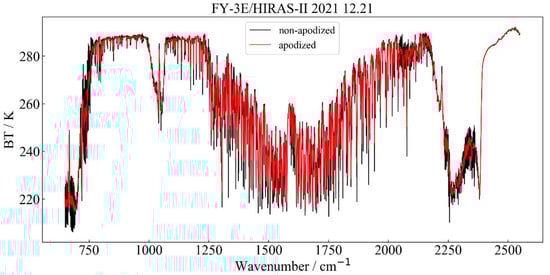
Figure 1.
Comparison of spectral brightness temperature before and after apodization.
In Figure 1, the black solid line presents the spectral brightness temperature without apodization and the red solid line presents the spectral brightness temperature after apodization. It can be seen that the burr phenomenon is reduced when the HIRAS spectrum undergoes apodization, and the spectrum is smoother.
- (2)
- Selection of clear sky pixels
Since the ERA reanalysis, data cannot guarantee sufficient accuracy for information such as clouds and precipitation, and the current simulation accuracy of RTTOV of clouds is not high, the sample data we selected in this experiment were all ocean clear sky field samples. In addition, the judgment conditions for our clear sky samples were as follows: in the experiment, we selected the observation data of 5 representative infrared channels (810, 830, 850, 870, and 890 cm−1) in the long-wave window region, whose brightness temperature is greater than 290 K, and the deviation of the observed brightness temperature from the simulated brightness temperature of the window channel should be less than 5 K. In addition, since the simulation results of RTTOV at higher latitudes are not very accurate [15], in this experiment, we selected clear sky ocean sample points located at middle and low latitudes.
2.2.2. Reanalysis Data Processing
Since the temporal and spatial resolutions of the ERA5 reanalysis data are different from the HIRAS-II and IASI observation data, before the reanalysis data were fed into the radiative transfer model for simulated brightness temperature calculations, we needed to interpolate the reanalysis data onto the temporal and spatial grids of satellite observations. For time interpolation, we took the time of the observation data as the criterion and selected the reanalysis data of two adjacent times for linear interpolation. For the spatial interpolation, we used the cubic spline interpolation algorithm to spatially interpolate the reanalysis data based on the geographic location information of the satellite observation data.
2.2.3. IASI Observation Data Processing
In order to quantitatively analyze the OMB double-difference comparison between HIRAS-II and IASI, we needed to match the time, spatial information, and spectrum of the observation data. Since the spectral resolution of IASI is higher than that of HIRAS-II, it was necessary to convert the spectral data of IASI to the spectroscopic specification of HIRAS-II, which was performed as follows.
- (1)
- Time and spatial match
The IASI data were selected according to the SNO cross-orbit forecast. Since most of the SNO orbital intersections are located in the polar regions, in order to ensure sufficient samples, we took the time of IASI observation data as the criterion and matched the HIRAS-II observation data within one hour before and after. According to the clear sky judgment criteria in Section 2.2.1, the clear sky observation samples were selected, the observation sample points of IASI and HIRAS-II located at middle- and low-latitude ocean areas were selected, and their regional positions were relatively fixed.
- (2)
- Spectral match
Both HIRAS-II and IASI are Fourier transform infrared spectrometers. According to the spectroscopic principle of Fourier interferometers, the spectral resolution of the observed signal is determined by the maximum optical path difference of the instrument. The original spectral resolution of IASI (unapodized) is 0.25 cm−1, whereas the spectral resolution of HIRAS-II is 0.625 cm−1, which is lower in comparison. In order to quantitatively compare the deviation of the two spectra, we needed to convert the high-resolution IASI spectrum to the low-resolution HIRAS-II spectrum. The specific conversion process was as follows.
First, we performed Fourier transform on the IASI spectrum to convert the frequency-domain spectrum into a time-domain interferogram. Secondly, we truncated the current IASI interferogram according to the HIRAS-II maximum optical path difference (OPD) and sampled it. Then, we removed the original Gaussian apodization function from the IASI interferogram. Figure 2 shows the comparison of the IASI interferogram after the de-apodization operation with the original interferogram; the deviation before and after the apodization can be seen more clearly in Figure 2b. Additionally, Figure 3 shows the deviation calculation result after taking the absolute value of the interferogram. It can be seen that there are more burrs in the interferogram after the de-apodization, especially in the vicinity of the OPD 0.6–0.8, the burr effect is more obvious. The deviation is relatively larger than that after the apodization when the OPD is about 0.6; the deviation of two reaches the maximum value, which is the same as the result shown in Figure 2.
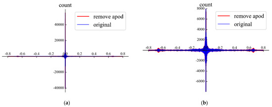
Figure 2.
IASI interferogram before and after apodization: (a) the blue line represents the original interferogram and the red line represents the interferogram after removing apodization. The abscissa is the optical path difference (OPD). (b) A partial enlarged image.
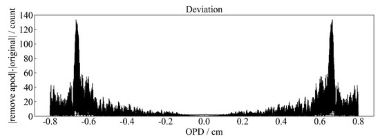
Figure 3.
IASI interferogram deviation comparison after apodization.
Next, we used IASI observations for the full day of 20 December 2021, and we performed inverse Fourier transform on the truncated interferogram to obtain the IASI spectrum of 0.625 cm−1, and finally, we used the Hamming function to apodize the IASI spectrum of 0.625 cm−1.
For both the observed and simulated IASI spectra, the same method was used for spectral conversion, as shown in Figure 4, to obtain the observed and simulated IASI spectra with a resolution of 0.625 cm−1.
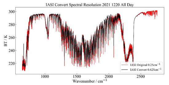
Figure 4.
Comparison before and after IASI spectral conversion.
2.2.4. Bias Evaluation Method
In this experiment, we used the ME (mean bias), the STD (standard deviation bias), and the DD [16] (double difference bias) as the accuracy evaluation criteria. The STD reflects the degree of deviation between the data; the smaller the standard deviation is, the stronger the stability between the data is, and the smaller the deviation characteristic is, the higher the precision is. The smaller the DD is, the more consistent the HIRAS and IASI observations are. The closer ME is to y = 0, the higher the accuracy is. The specific calculation formulas are as follows:
where xi is the observed value, xi′ is the simulated value, and n is the number of samples.
3. Results Analysis
Based on the above analysis methods, we selected typical spectral channels in the three infrared bands of HIRAS-II to conduct an OMB bias analysis. FY-3E/HIRAS-II had a total of 9 FOVs (pixels for the field of view), named FOV1–FOV9. Since the on-orbit test found that the sensitivity of FOV1 of the HIRAS-II short-wave infrared detector exceeded the index requirements, in this experiment, we eliminated the observation samples of FOV1 and only analyzed and evaluated the observation samples of the other FOVs.
3.1. FY-3E/HIRAS-II Overall Bias of OMB Distribution
We selected FY-3E/HIRAS-II ocean clear sky field data according to the method in Section 2.2.1 and calculated the ME and STD between the FY-3E/HIRAS-II observation and simulation. We used HIRAS-II observations for the full day of 21 December 2021. The results are shown in Figure 5 and Figure 6 below; among them, Figure 6 is based on the statistics of all samples of 8 FOVs.
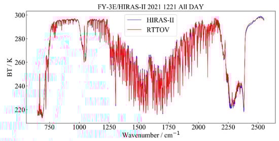
Figure 5.
Comparison of FY-3E/HIRAS-II observed and simulated brightness temperature.
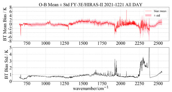
Figure 6.
ME and STD of FY-3E/HIRAS-II observations and simulations.
In Figure 5, the blue curve is the observed brightness temperature of HIRAS-II and the red curve is the HIRAS-II simulated brightness temperature obtained by RTTOV. The observed brightness temperature was generally consistent with the simulated brightness temperature.
The red line in Figure 6 represents the mean bias of brightness temperature between the HIRAS-II observation and simulation, the pink shading represents the one-time STD fluctuation interval, and the black line is the OMB standard bias. Figure 6 shows that the ME of OMB in the long-wave and medium-wave infrared bands is ±1 K, except for the CO2 absorption band around 680 cm−1 and the ozone absorption band around 1000 cm−1. In addition, the bias of the medium wave from 1600 to 1750 cm−1 fluctuates strongly, and we considered that the water vapor profile of ERA5 may be overestimated in the middle troposphere, which led to an error of about 2 K in the medium-wave water vapor absorption [7]. From Figure 6, it can also be seen that the ME was in the range of ±2 K overall near the short wave and was greater than 5 K in some channels at 2250–2400 cm−1. A subsequent detailed analysis of each FOV was carried out to check the deviation distribution of each FOV in the short wave.
3.2. The Bias of OMB Global Sample Distribution
We selected six typical channels to analyze the variation distribution characteristics of the bias between observation and simulation on the global spatial scale. The relevant results are shown in Figure 7, where the color depth indicates the magnitude of the bias, and the channels we selected were 680, 900, 1400, 1600, 2200, and 2500 cm−1.
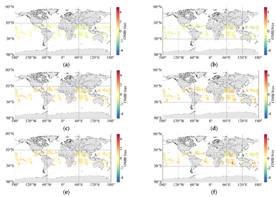
Figure 7.
Distribution map of global biased samples: (a) 680 cm−1; (b) 900 cm−1; (c) 1400 cm−1; (d) 1600 cm−1; (e) 2200 cm−1; and (f) 2500 cm−1.
In the global distribution of the bias of OMB, the bias of the long-wave 900 cm−1 channel is the smallest, and the medium-wave 1400 cm−1 deviation was similar to that of 900 cm−1. Furthermore, we found that the OMB had a large bias on one side of the track at 2500 cm−1, which was due to the influence of sun glint on the channel near 2500 cm−1, resulting in a high value of the observed radiation in Figure 7. The RTTOV model simulation, however, did not consider this phenomenon, which eventually caused the bias of OMB in the range of 2400–2550 cm−1 to be larger. The calculation of the sun glint angle [17,18] was as follows:
where is the solar flare angle; and are the solar zenith angle and satellite zenith angle, respectively; and and are the solar azimuth and satellite azimuth, respectively.
We used the cubic spline regression fitting algorithm to solve the contribution of sun glint to OMB [18]. The relevant calculation method is as follows:
where O − B is the bias between observation and simulation; is the channel wavenumber; and , , , and are the fitting coefficients in the cubic regression.
In Figure 8, the color of the sample point represents its probability density. The redder the color is, the higher the frequency of the sample in this angle range is. The red curve represents the relationship between the bias of OMB and the sun glint angle fitted by the cubic spline algorithm. It can be seen from Figure 8 that the bias of OMB gradually decreased with the increase in the sun glint angle, and the bias dropped to 0 at approximately 40 degrees. Moreover, the smaller the sun glint angle is, the larger the bias of the short-wave range of 2400–2500 cm−1 is, and the cubic polynomial curve can well fit the sun glint angle and the radiation deviation contributed by it. In order to better show the impact of sun glint on the L1 data, we compared the HIRAS-II spectral brightness temperature data on 21 December 2021 with the sun glint angle calculated by Formula (5).
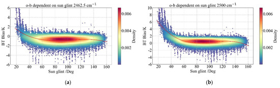
Figure 8.
Fitting relationship between sun glint angle and the bias of OMB. (a) 2462.5 cm−1; (b) 2500 cm−1.
Comparing the distribution of global brightness temperature values and global sun glint angles at 2500 cm−1, we can see that since HIRAS-II performs cross-orbit scanning along the line of dawn and dusk, the areas with sun glint angles of less than 40 degrees were mostly concentrated on one side of the orbit (with illumination) in Figure 9. The observed brightness temperature values of HIRAS-II on this side were relatively high, resulting in a large OMB bias of the global sample on this side. In the future, we will correct the OMB bias at 2400–2550 cm−1 based on the cubic spline regression curve to further reduce the impact of solar flares, which will be beneficial to business data applications. In the following chapters, in the short-wave 2400–2550 cm−1 channel range, we have eliminated samples with solar flare angles of less than 40 degrees.
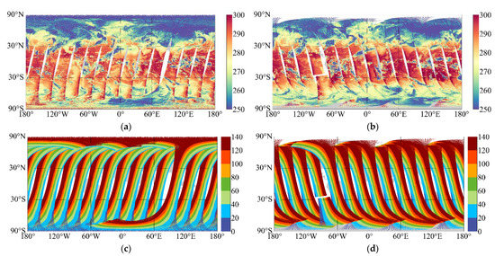
Figure 9.
(a,b) are the brightness temperature values of the ascending orbit and descending orbit of 2500 cm−1, respectively; (c,d) show the global distribution of sun glint angles for the ascending and descending orbits of HIRAS-II, respectively.
3.3. Analysis of the OMB Consistency of Each FOV in FY-3E/HIRAS-II
FY-3E/HIRAS-II had a total of nine FOVs, the instantaneous field of view to the ground was 14 km, and the angle of each detector to the ground was 1°. The arrangement of the nine FOVs is shown in Figure 10. In order to assess the consistency of the bias between individual detectors, we separated the FOV samples of FY-3E/HIRAS-II for OMB bias statistics.
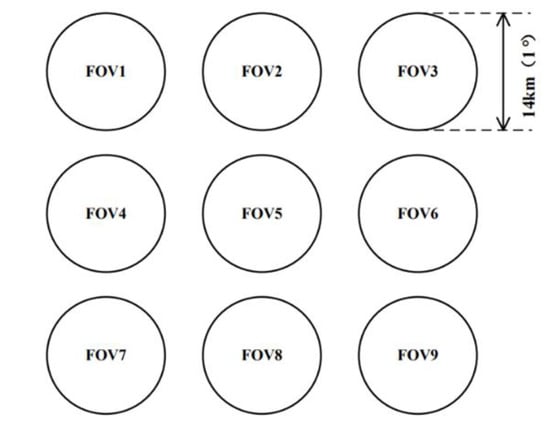
Figure 10.
Illustration of the arrangement of the ground field of view for each detector (3 × 3 FOVs).
As shown in Figure 10, the nine FOVs of HIRAS-II were arranged in a 3 × 3 array. We selected the observation data and simulation data of the ocean clear sky field of view on 21 December 2021, classified the samples according to each FOV, eliminated FOV1 with poor sensitivity, and counted the mean bias of OMB and the standard deviation of OMB of the FOV2-FOV9 samples. The result is shown in Figure 11.
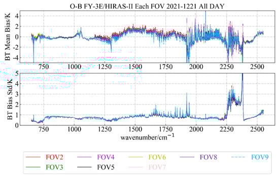
Figure 11.
Mean bias of OMB and standard deviation of OMB between individual FOVs.
From Figure 11, we found that in the long-wave infrared band, the mean bias of OMB of FOV2-FOV9 was distributed around y = 0, and the standard deviation was generally better than 1 K. In the medium-wave infrared band, both the ME and STD were lower than 2 K, and FOV9 had a small deviation in the water vapor absorption band. In the short-wave infrared band, the mean bias of OMB was ±4 K, and the STD was less than 2 K in most channels.
In order to examine the consistency between each FOV, we subtracted the center detector FOV5 from FOV2 to FOV9. The results are shown in Figure 12. The consistency between the long-wave detectors was good, better than 0.5 K, and most channels are excellent at 0 K. In the medium-wave range, most FOV channels except FOV9 were better than 0.5 K, and FOV9 was mostly better than 1 K. Most of the short-wave FOV channels were also better than 2 K. Only the bias near 2000 and 2300 cm−1 was greater than 2 K. This was related to the simulation accuracy of the radiation transfer mode. We will explain the relevant phenomena in detail in the follow-up analysis.
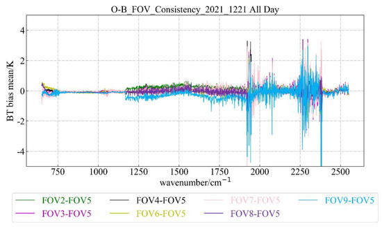
Figure 12.
Consistency of mean bias of OMB across each FOV.
3.4. Analysis of Bias of OMB with Scanning Angle Change of FY-3E/HIRAS-II Instrument
FY-3E/HIRAS-II contained a total of 28 ground scans in a single scan cycle—that is, it had 28 resident FORs—and the scanning angle range is 100.8°—that is, its maximum scanning angle was ±50.4°. We used data from ocean clear sky field observations and simulations on 21 December 2021 and calculated the mean bias of OMB of typical channels (680, 900, 1350, 1600, 2200, and 2500 cm−1) with the scanning angle, as shown in the following figure.
As shown in Figure 13, the mean bias of OMB of the typical channels we selected was better than 1 K at each scanning angle overall, and the long-wave 900 cm−1 channel had the most stable performance and was distributed around y = 0. The STDs of all channels were better than 1 K at every scan angle; the best performing was 680 cm−1, and the STDs were smoothly distributed at 0.5 K. We found that although the ME and STD of OMB were relatively small, there was still inconsistency in the variation of the deviation of the long-wave, medium-wave, and short-wave infrared bands with the satellite scanning angle, so each band was analyzed separately.
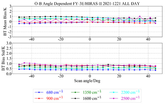
Figure 13.
The distribution of the bias of a typical channel with the scanning angle.
For the long-wave channels, we selected 680, 750, 800, 850, 900, 1000, and 1100 cm−1 for analysis. The results are shown in the following figure.
As can be seen from Figure 14 and Figure 15, the mean bias of OMB range of each FOV of the long-wave channels is ±2 K, the STD was less than 1 K, and the bias of OMB does not change with the angle, which was relatively stable.
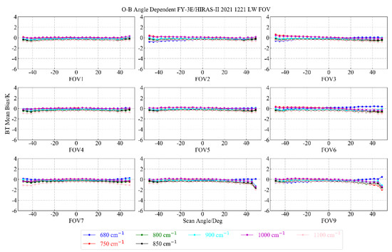
Figure 14.
Distribution of mean bias of OMB values of 9 FOVs of typical long-wave channels as a function of scanning angle.
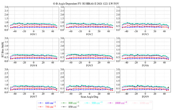
Figure 15.
Distribution of OMB standard deviation of 9 FOVs of typical long-wave channels as a function of scanning angle.
For the medium wave channel, we selected 1300 cm−1, 1400 cm−1, 1500 cm−1, 1600 cm−1, 1660 cm−1, 1700 cm−1, and 1750 cm−1 for analysis. The results are shown in the following figure.
It can be seen from Figure 16 and Figure 17 that the overall ME range of each FOV in a typical medium-wave channel was ±2 K, only the 1300 and 1700 cm−1 channels had a value greater than 2 K at FOV9, and the STD was lower than 1.5 K in most channels.
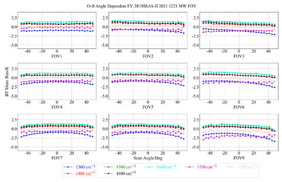
Figure 16.
Distribution of mean bias of OMB values of 9 FOVs of typical medium-wave channels as a function of scanning angle.
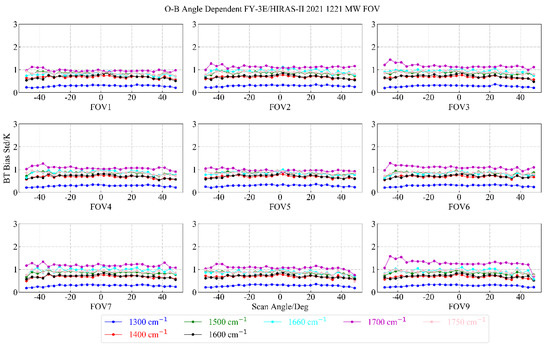
Figure 17.
Distribution of OMB standard deviation of 9 FOVs of typical medium-wave channels as a function of scanning angle.
For the short-wave channels, we selected 2100, 2200, 2250, 2300, 2350, 2400, and 2500 cm−1 for analysis, and we excluded FOV1 samples with poor sensitivity. The results are shown in the following figure.
It can be seen from Figure 18 and Figure 19 that there is a large mean bias of OMB at 2300 and 2350 cm−1, which is similar to the phenomenon before CrIS (Cross-Track Infrared Sounder) is corrected for non-local thermodynamic equilibrium (NLTE), the o-b of CrIS is affected by NLTE at daytime, the deviation is above 3 K, and its STD is around 2 K [19]. Therefore, we infer that it may be caused by the NLTE of the upper atmosphere, and the NLTE of HIRAS-II is not simulated in RTTOV. In the later stage, the focus of our OMB analysis will be on the NLTE of the upper atmosphere at 2200–2300 cm−1 [12]. In addition, as shown in Figure 18, the mean bias of OMB at 2500 cm−1 also has a sawtooth fluctuation with the change of the scanning angle; the reason for this phenomenon is still under investigation.
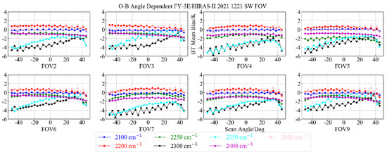
Figure 18.
Distribution of mean bias of OMB values of 9 FOVs of typical short-wave channels as a function of scanning angle.
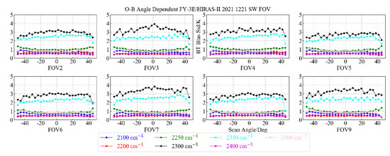
Figure 19.
Distribution of OMB standard deviation of 9 FOVs of typical short-wave channels as a function of scanning angle.
3.5. Analysis of the Change of the Bias of OMB with Day and Night
FY-3E is a dawn and dusk orbit satellite that scans across the orbit along the Earth’s culmination circle. We used the size of the satellite’s zenith angle to determine whether the observation data are daytime or nighttime data. Our rules for selecting data were as follows: when the satellite zenith angle is less than 80°, the samples are regarded as daytime samples; a sample with a satellite zenith angle of 80 to 90° is regarded as a sample near the line of dawn and dusk; and when the satellite zenith angle is greater than 90°, the observation samples are regarded as night samples. The relevant analysis results are shown below.
As can be seen from Figure 20, in the long-wave and medium-wave bands, we found that the changes in the mean bias of OMB values of the daytime, line of dawn and dusk, and nighttime samples were relatively consistent, and the bias of the short-wave nighttime samples had a smaller error than the daytime samples. On the short-wave side, we found that the mean bias of OMB at 2200–2300 cm−1 differed between day and night. This phenomenon has been pointed out in the relevant literature, and the NLTE of daytime at the short-wave range of 2200–2300 cm−1 exists from 2 km near the ground to the top of the atmosphere, while the NLTE of the night starts from the upper stratosphere to the top of the atmosphere, resulting in a significant difference in radiation between the daytime and nighttime [20].
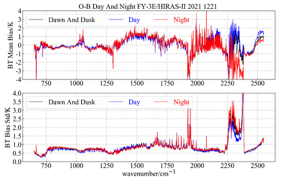
Figure 20.
The bias of OMB distribution during day and night.
3.6. Analysis of the Bias of OMB Variation with Observation Target Temperature
FY-3E/HIRAS-II uses the internal calibration target as the hot target and the deep space as the cold target for radiation calibration. This calibration method is based on the linear response of the instrument to the incident radiation. In actual observations, the response of the instrument relative to the incident radiation was non-linear. Zou [21] and Saunders [22] believed that the non-linear characteristic of this instrument is the main reason for the dependence of bias on the observation target temperature. We selected six typical channels of HIRAS-II, namely 680, 900, 1350, 1600, 2200, and 2500 cm−1, to check the change in bias in typical channels with the observation target temperature.
As shown in Figure 21 above, we found that the bias of OMB distribution of most typical channels was relatively stable with the target temperature. The typical long-wave and medium-wave channels did not have an obvious bias that depended on temperature, and the overall bias was stable within 1 K, which proves that HIRAS-II does not have obvious non-linear effects. The bias of the 2500 cm−1 channel was relatively stable with the target temperature, which is related to the exclusion of data affected by sun glint. When the variation with the target temperature, the source of the deviation does not necessarily come from the non-linear effect of the instrument, so it is necessary to remove the sun glint effect in the experiment.
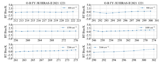
Figure 21.
The bias of OMB distribution with target temperature.
3.7. Analysis of the Bias of OMB Variation with Ascending Orbit and Descending Orbit
In order to check the distribution of bias between the ascending and descending orbits of the instrument [23], we divided the observation samples into samples of the ascending and descending orbits and examined the OMB bias changes of both orbits with the scanning angle of the instrument. We also checked the bias distribution between the ascending and descending orbits during the day and night.
In Figure 22, the different colors represent different channels. Regarding the change in the mean OMB bias value with the scanning angle of HIRAS-II, the bias of the descending orbit and ascending orbit at 2500 cm−1 is inconsistent in distribution around +48°. The bias of the ascending orbit around +48° was larger than that of the descending orbit, but the overall value was within 2 K. In terms of STD, the error of the descending orbit was smaller than that of the ascending orbit and the distribution was more stable.
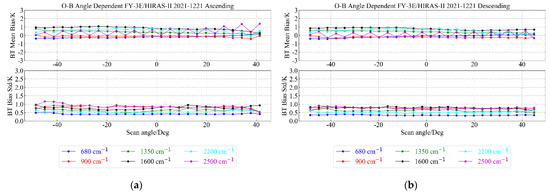
Figure 22.
The distribution of the bias of a typical channel with the scanning angle: (a) the ascending orbit samples; (b) the descending orbit samples.
In Figure 23, the blue line indicates the bias between the ascending and descending orbits during the day, and the red line indicates the bias between the ascending and descending orbits during the night. We can see that the bias trended between the ascending and descending orbits during the day and night were roughly the same. In the long-wave and medium-wave ranges, the largest bias was within ±0.5 K. For the short-wave range there was a 1 K bias of the ascending and descending orbits around 2300 cm−1 during daytime and nighttime. The issue of the inconsistency of the bias between the ascending and descending orbit data needs to be studied.
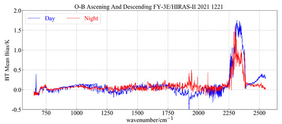
Figure 23.
Comparison of the bias between the ascending and descending orbit during the day and night.
3.8. Analysis of the Bias of OMB Variation with Latitude
To assess the radiometric calibration consistency of HIRAS-II between different latitudes [24,25], we selected six typical channels (680, 900, 1350, 1600, 2200, and 2500 cm−1) to analyze the variation in the bias of HIRAS-II with latitude.
As shown in Figure 24 above, under the clear sky selection conditions we set in this experiment were mostly targets with higher temperatures; the latitude of the sample was within the range of ±40° north and south latitudes, and the bias of 2500 cm−1 was symmetrical with the distribution of latitude at 2 K. The bias of OMB of most latitude locations was within 1 K. The bias distribution of the other typical channels showed no obvious change with latitude, was relatively stable, and had no obvious latitude-dependent characteristics.
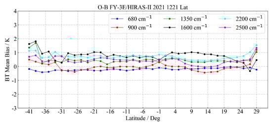
Figure 24.
Schematic diagram of the variation in the bias of OMB with latitude.
3.9. Evaluation of Calibration Accuracy and Stability of FY-3E/HIRAS-II Based on OMB
In this experiment, we calculated the bias of OMB changes on a daily basis from 24 November 2021 to 15 January 2022 and selected typical channels (680, 900, 1400, 1600, 2200, and 2500 cm−1) to view the long-term changes in OMB over time.
In Figure 25 above, the dots represent the daily mean bias of OMB. Due to some action arrangements during the on-orbit test of HIRAS-II, the quality of L1 data will be low, so we deleted the data of the time nodes when HIRAS-II had actions. According to the results, the mean bias value of most typical channels was less than 1 K for a long time, and the bias distribution was relatively stable, indicating that the radiation calibration effect of HIRAS-II was relatively stable. Among them, the bias of the long-wave channels 680 and 900 cm−1 was the best, fluctuating around y = 0; the other channels were stable overall, and there was no major deviation change.
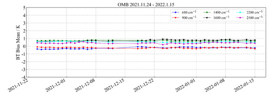
Figure 25.
Distribution of the bias of OMB over time.
We then counted the OMB standard deviation of each channel from 24 to 30 November 2021, which was defined as the stability of the calibration accuracy of the channel. The better the calibration accuracy and stability are, the better the radiometric calibration accuracy and stability are, which is conducive to the later development of related experiments such as assimilation and retrieval applications based on HIRAS-II.
In Figure 26 above, the lines of different colors represent different FOVs. We found that the calibration accuracy stability of most channels in each FOV is within 0.1 K. Due to the influence of the ozone absorption line, the OMB standard deviation has a small peak near 1000 cm−1, but it is still better than 0.1 K. The bias of FOV9 around 1900 cm−1 of the medium wave is about 0.2 K. The calibration accuracy of the other channels is high, all below 0.1 K. For the short wave near 2300 cm−1, the RTTOV model does not consider the NLTE of the upper atmosphere, resulting in a standard deviation of 0.3 K, but most channels have a high calibration accuracy and stability.
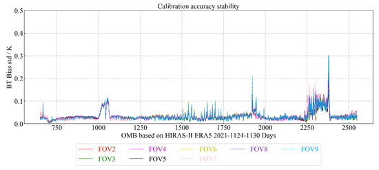
Figure 26.
Calibration accuracy and stability of FY-3E/HIRAS-II.
3.10. Double-Difference Alignment with IASI’s Bias of OMB Results
In order to assess whether the deviations of HIRAS-II and IASI observations and simulations are consistent, we used the selection method of IASI data in Section 2.2.3, and we used the observation data and simulation data of MetOp-C/IASI and FY-3E/HIRAS-II on 20 December 2021. We will count and analyze MetOp-C/IASI and FY-3E/HIRAS-II their respective OMB deviations and finally calculate the double difference of deviations between the two. The double difference in the bias result is shown in Figure 26, below.
As shown in Figure 27 above, there are different degrees of bias between the two instruments in the short-wave infrared band. We consider that the reason for the large bias in the OMB near the short-wave range of 2200–2300 cm−1 is the poor simulation accuracy of the radiative transfer mode (without considering the NLTE), resulting in a large bias of the double difference. In the long-wave and medium-wave bands, the OMB double difference results of HIRAS-II and IASI show a similar trend. Except for the CO2 absorption band of 680–750 cm−1, the bias of the other long-wave channels is lower than 0.5 K. Most of the medium-wave channels perform well—the double difference is stable within 1 K, and some channels are better than 0.5 K. It shows that HIRAS-II has high precision in radiometric calibration.
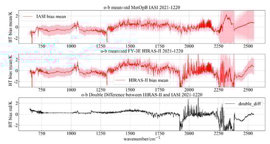
Figure 27.
Comparison of HIRAS-II and IASI double difference.
4. Discussion
Using OMB to evaluate the radiometric calibration performance of infrared hyperspectral instruments is one of the key tasks before infrared hyperspectral data are input into a numerical prediction system. In this experiment, we calculated the ME and STD of OMB based on FY-3E/HIRAS-II and the simulation results of RTTOV. The findings from our evaluation are detailed below.
Firstly, since the simulation of NLTE in RTTOV only exists in the IASI sensor coefficient file [26], the NLTE observed by HIRAS-II is not effectively simulated in RTTOV, resulting in a large bias of OMB from 2200 to 2300 cm−1. Related research [27] also confirmed that there is a large difference between the daytime and nighttime NLTE. Therefore, if we obtain the sensor coefficient file of HIRAS-II with NLTE simulation in the future, we will perform OMB statistical calculation on HIRAS-II.
Secondly, we found that there was a sun glint effect in the short-wave range from 2400 to 2500 cm−1, but RTTOV did not simulate this effect, resulting in a large bias of OMB in these channels. Therefore, we deleted the observation samples affected by sun glint. Sun glint effects are an important factor affecting the accuracy of radiometric calibration. Later, we will use cubic polynomial regression to correct the observation data [17,18] so that the observation data can be used by global numerical prediction models.
There are still some phenomena that we need to continue to improve in follow-up work. For example, in the analysis of Section 3.4, there is a sawtooth phenomenon in the OMB near the short-wave channel 2500 cm−1 with the scanning angle, which may be related to the accuracy of spectral calibration or radiometric calibration, and this part of the phenomenon will be the focus of later research. Additionally, in Section 3.7, the OMB still has a certain bias between the ascending and descending orbits, and this will also be the focus of later research. In this study, the source of the OMB bias is not only the error of instrument observation but also some errors in the RTTOV model as well as the input profile and the interpolation algorithm, which together lead to the generation of the bias. In the follow-up experiments, we will further combine the physical characteristics of the phenomenon of OMB and conduct a more detailed analysis and explanation of the source of the bias of OMB, so as to improve the application prospect of HIRAS-II.
5. Conclusions
FY-3E is China and the world’s first civil operational meteorological satellite in sun-synchronous dawn and dusk orbit. The radiometric calibration accuracy of HIRAS-II is related to the assimilation effect of its data entering the numerical prediction model. Therefore, we need to quantitatively analyze the bias characteristics and evaluate the accuracy of the radiometric calibration. In this paper, we used the FY-3E/HIRAS-II observation data and the simulation results of RTTOV to calculate the bias of OMB of the two, and we calculated a double-difference comparison between the OMB of HIRAS-II and the OMB of IASI. We obtained the following preliminary conclusions.
The HIRAS-II radiometric calibration accuracy performed well during the on-orbit test. The bias between the FOVs in the long-wave and medium-wave bands was better than 2 K, with good consistency, and the mean OMB bias value changed with the scanning angle of the instrument and was better than 1 K. The mean OMB and STD are consistent with daytime and nighttime changes in long-wave and medium-wave bands. The reason for the inconsistency of the short-wave bias is that the RTTOV model does not consider the NLTE phenomenon.
Through experiments, we found that the bias of OMB does not change significantly with the target temperature, and the non-linear effect of the instrument is well corrected. We then analyzed the variation in the bias with latitude, and the experiments showed that the bias of OMB had no obvious latitude-dependent characteristics. Immediately afterwards, we found that there is still an inconsistency of about 1 K bias in some channels (near 1900 and 2300 cm−1) between the ascending and descending orbits, which will be further analyzed later.
We calculated the OMB bias of the HIRAS-II observation data for one month, and most of the channel bias changes were less than 0.1 K, showing good stability. Then, we used the HIRAS-II data of one week to calculate the STD of bias of all channels and obtained the calibration accuracy stability. The test showed that the calibration accuracy stability of most channels is better than 0.1 K. Therefore, the above experiments show that HIRAS-II has a highly stable radiometric calibration accuracy.
Finally, we performed a double-difference comparison with the bias of IASI’s OMB, and the double difference was better than 0.5 K near the long-wave and medium-wave bands. At the short-wave channel 2300 cm−1, some errors occurred because the RTTOV simulation did not consider the NLTE, but the magnitude of the double-difference bias was better than ±2 K.
In this experiment, we conducted a comprehensive evaluation of the radiometric calibration accuracy of HIRAS-II based on OMB bias analysis. The analysis of the above experiments showed that HIRAS-II has a high radiometric calibration accuracy. At the same time, our work can provide an important reference for the quantitative application of HIRAS-II data as well as a basis for subsequent instrument development and data preprocessing algorithm improvement. It can also provide a more detailed reference for HIRAS-II to enter the global numerical prediction model and assimilation systems.
Author Contributions
Conceptualization, C.Z., C.Q. and T.Y.; methodology, C.Z. and C.Q.; software, C.Z. and P.Z.; validation, C.Z., C.Q., T.Y., M.X. and L.L.; formal analysis, C.Z., C.Q. and P.Z.; investigation, C.Z., C.Q. and T.Y.; resources, C.Z.; data curation, C.Q., L.L. and X.H.; writing—original draft preparation, C.Z., C.Q. and T.Y.; writing—review and editing, C.Z., M.G. and M.X.; visualization, C.Q. and X.H.; supervision, M.G. and X.H.; project administration, C.Q.; funding acquisition, C.Q. and M.G. All authors have read and agreed to the published version of the manuscript.
Funding
This research was funded by the National Key R&D Program of China (2018YFB0504800 (2018YFB0504802)), National Key R&D Program of China (2018YFB0504700 (2018YFB0504703)), and Fengyun Satellite Application Pilot Project (FY-APP-2021.0507).
Data Availability Statement
All data generated or analyzed during this study are included in this article.
Acknowledgments
We would like to thank the NSMC (National Satellite Meteorological Center) for sharing FY3E/HIRAS-II data. We would also like to thank the ECMWF for their openly accessible data and software and Chunqiang Wu from the NSMC, CMA (China Meteorological Administration), for providing the RTTOV coefficient file on FY-3E/HIRAS-II.
Conflicts of Interest
The authors declare no conflict of interest.
References
- Sun, L.; Guo, M.H.; Xu, N.; Zhang, L.J.; Liu, J.J.; Hu, X.Q.; Li, Y.; Rong, Z.G.; Zhao, Z.H. On-Orbit Response Variation Analysis of FY-3 MERSI Reflective Solar Bands Based on Dunhuang Site Calibration. J. Spectrosc. Spectral. Anal. 2012, 32, 1869–1877. [Google Scholar]
- Min, M.; Zhang, Y.; Hu, X.Q.; Dong, L.X.; Rong, Z.G. Evaluation for radiometric calibration of infrared band of FY-3A medium resolution spectral imager (MERSI) using radiometric calibration sites. J. Infrared Laser Eng. 2012, 41, 1995–2001. [Google Scholar]
- Loew, A.; Bell, W.; Brocca, L.; Bulgin, C.E.; Burdanowitz, J.; Calbet, X.; Donner, R.V.; Ghent, D.; Gruber, A.; Kaminski, T.; et al. Validation practices for satellite-based Earth observation data across communities. J. Rev. Geophys. 2017, 55, 779–817. [Google Scholar] [CrossRef] [Green Version]
- Yang, T.H.; Hu, X.Q.; Xu, H.L.; Wu, C.Q.; Qi, C.L.; Gu, M.J. Radiation Calibration Accuracy Assessment of FY-3D Hyper-spectral Infrared Atmospheric Sounder Based on Inter-Comparison. Acta Opt. Sin. 2019, 39, 377–387. [Google Scholar]
- Yang, T.H. Tropospheric Wind Field Measurement Based on Infrared Hyperspectral Observations. Ph.D. Thesis, University of Chinese Academy of Sciences, Beijing, China, 2020. [Google Scholar]
- Wang, L.; Han, Y.; Jin, X.; Chen, Y.; Tremblay, D.A. Radiometric Consistency Assessment of Hyperspectral Infrared Sounders. Atmos. Meas. Tech. 2015, 8, 4831–4844. [Google Scholar] [CrossRef] [Green Version]
- Qu, J.H.; Zhang, L.; Lu, Q.F.; Zhang, N.Q.; Wang, D. Characterization of bias in FY-4A advanced geostationary radiation imager observation from ERA5 background simulation using RTTOV. J. Acta Meteorol. Sin. 2019, 77, 911–922. [Google Scholar]
- Xu, N.; Chen, L.; Hu, X.Q.; Zhang, L.Y.; Zhang, P. Assessment and correction of on-orbit radiometric calibration for FY-3 VIRR thermal infrared channels. J. Remote Sens. 2014, 6, 2884–2897. [Google Scholar] [CrossRef] [Green Version]
- Zhang, P.; Hu, X.Q.; Lu, Q.F.; Zhu, A.J.; Lin, M.Y.; Sun, L.; Chen, L.; Xu, N. FY-3E: The First Operational Meteorological Satellite Mission in an Early Morning Orbit. J. Adv. Atmos. Sci. 2022, 39, 1–8. [Google Scholar] [CrossRef]
- Lee, L.; Wu, C.Q.; Qi, C.L.; Hu, X.Q.; Yuan, M.G. Solar Contamination on HIRAS Cold Calibration View and the Corrected Radiance Assessment. J. Remote Sens. 2022, 13, 19. [Google Scholar] [CrossRef]
- Holmlund, K.; Bojkov, B.; Klaes, D.; Schlussel, P. The Joint Polar System: Towards the Second Generation EUMETSAT Polar System. In Proceedings of the 2017 IEEE International Geoscience and Remote Sensing Symposium (IGARSS), Fort Worth, TX, USA, 23–28 July 2017; pp. 2779–2782. [Google Scholar]
- Hilton, F.; Armante, R.; August, T.; Barnet, C.; Bouchard, A.; Camy-Peyret, C.; Capelle, V.; Clarisse, L.; Clerbaux, C.; Coheur, P.-L.; et al. Hyperspectral Earth Observation from IASI Five Years of Accomplishments. Bull. Am. Meteorol. Soc. 2012, 93, 347–370. [Google Scholar] [CrossRef]
- Di, D. Data Assimilation Research for Geosynchronous Interferometric Infrared Sounder onboard FengYun-4 Satellite. Ph.D. Thesis, University of Chinese Academy of Sciences, Beijing, China, 2019. [Google Scholar]
- Zhang, C.M.; Gu, M.J.; Hu, Y.; Huang, P.Y.; Yang, T.H.; Huang, S.; Yang, C.L.; Shao, C.Y. A study on the retrieval of temperature and humidity profiles based on FY-3D/HIRAS infrared hyperspectral data. J. Remote Sens. 2021, 13, 2157. [Google Scholar] [CrossRef]
- Newman, S.; Carminati, F.; Lawrence, H.; Bormann, N.; Salonen, K.; Bell, W. Assessment of New Satellite Missions within the Framework of Numerical Weather Prediction. J. Remote Sens. 2020, 12, 1580. [Google Scholar] [CrossRef]
- Wang, L.K.; Goldberg, M.; Wu, X.Q.; Cao, C.Y.; Iacovazzi, R.A.; Yu, F.F.; Li, Y.P. Consistency assessment of Atmospheric Infrared Sounder and Infrared Atmospheric Sounding Interferometer radiances: Double differences versus simultaneous nadir overpasses. J. Geophys. Res.-Atmos. 2011, 116, D11. [Google Scholar] [CrossRef]
- Yin, M.T. Assessing the Sun Glint Effect on the Data Bias of CrIS Shortwave Surface Channels near 3.7 μm. Int. J. Remote Sens. 2016, 37, 356–369. [Google Scholar] [CrossRef]
- Wang, L.W.; Niu, Z.Y.; Zhang, B.L.; Tang, F.; Liang, J.H. A test of a sun glint correction method for the near-3.9 μm channels of the FengYun-3D Hyperspectral InfraRed Atmospheric Sounder (HIRAS). Remote Sens. Lett. 2020, 11, 943–951. [Google Scholar] [CrossRef]
- Yin, M.T. Bias characterization of CrIS shortwave temperature sounding channels using fast NLTE model and GFS forecast field. J. Geophys. Res.-Atmos. 2016, 121, 1248–1263. [Google Scholar] [CrossRef] [Green Version]
- Tan, P.F.; Han, Y.G.; Xuan, Y.M. Analysis of the Non-local Thermodynamic Equilibrium Effect on Infrared Limb Radiances in the Upper Atmosphere. J. Acta Opt. Sin. 2014, 34, 9–15. [Google Scholar]
- Zou, X.; Zhuge, X.; Weng, F. Characterization of bias of advanced Himawari imager infrared observation from NWP back-ground simulations using CRTM and RTTOV. J. Atmos. Ocean Technol. 2016, 33, 2553–2567. [Google Scholar] [CrossRef]
- Saunders, R.W.; Blackmore, T.A.; Candy, B.; Francis, P.N.; Hewison, T.J. Monitoring satellite radiance biases using NWP models. IEEE Trans. Geosci. Remote Sens. 2013, 51, 1124–1138. [Google Scholar] [CrossRef]
- Xie, X.X.; Wu, S.L.; Xu, H.X.; Yu, W.M.; He, J.K.; Gu, S.Y. Ascending-Descending Bias Correction of Microwave Radiation Imager on Board FengYun-3C. IEEE Trans. Geosci. Remote Sens. 2019, 57, 3126–3134. [Google Scholar] [CrossRef]
- Adler-Golden, S.; Smith, D.R.; Vail, J.; Berk, A.; Nadile, R.; Jeong, L. Simulations of mesospheric and thermospheric IR radiance measured in the CIRRIS-1 A shuttle experiment. J. Atmos. Solar-Terr. Phys. 1999, 61, 1397–1410. [Google Scholar] [CrossRef]
- Lu, Q.; Hu, J.; Wu, C.; Qi, C.; Wu, S.; Xu, N.; Sun, L.; Lia, X.; Liu, H.; Guo, Y.; et al. Monitoring the performance of the Fengyun satellite instruments using radiative transfer models and NWP fields. J. Quant. Spectrosc. Radiat. Transfer. 2020, 255, 107239. [Google Scholar] [CrossRef]
- Saunders, R.; Hocking, J.; Turner, E.; Rayer, P.; Rundle, D.; Brunel, P.; Vidot, J.; Roquet, P.; Matricardi, M.; Geer, A.; et al. An update on the RTTOV fast radiative transfer model (currently at version 12), Geosci. Model Dev. 2018, 11, 2717–2737. [Google Scholar] [CrossRef] [Green Version]
- Kay, S.; Hedley, J.D.; Lavender, S. Sun Glint Correction of High and Low Spatial Resolution Images of Aquatic Scenes: A Review of Methods for Visible and Near-Infrared Wavelengths. J. Remote Sens. 2009, 1, 697–730. [Google Scholar] [CrossRef] [Green Version]
Publisher’s Note: MDPI stays neutral with regard to jurisdictional claims in published maps and institutional affiliations. |
© 2022 by the authors. Licensee MDPI, Basel, Switzerland. This article is an open access article distributed under the terms and conditions of the Creative Commons Attribution (CC BY) license (https://creativecommons.org/licenses/by/4.0/).