AC-LSTM: Anomaly State Perception of Infrared Point Targets Based on CNN+LSTM

Abstract

Anomaly perception of infrared point targets has high application value in many fields, such as maritime surveillance, airspace surveillance, and early warning systems. This kind of abnormality includes the explosion of the target, the separation between stages, the disintegration caused by the abnormal strike, etc. By extracting the radiation characteristics of continuous frame targets, it is possible to analyze and warn the target state in time. Most anomaly detection methods adopt traditional outlier detection, which has the problems of poor accuracy and a high false alarm rate. Driven by data, this paper proposes a new network structure, called AC-LSTM, which combines Convolutional Neural Networks (CNN) with Long Short-Term Memory (LSTM), and embeds the Periodic Time Series Data Attention module (PTSA). The network can better extract the spatial and temporal characteristics of one-dimensional time series data, and the PTSA module can consider the periodic characteristics of the target in the process of continuous movement, and focus on abnormal data. In addition, this paper also proposes a new time series data enhancement method, which slices and re-amplifies the long time series data. This method significantly improves the accuracy of anomaly detection. Through a large number of experiments, AC-LSTM has achieved higher scores on our collected datasets than other methods.

1. Introduction

Infrared images are obtained by “measuring” the radiant heat of the object or scene [1]. Infrared images are often used to dynamically observe and capture objects such as drones and helicopters. During the flight of the above target, many abnormal states may occur, such as the unusual trajectory of the target due to unexpected mechanical malfunction, and explosion or disintegration of the target due to its cause or abnormal strike. These states are categorized as abnormal events that differ from the normal flight state. The target’s radiated energy and flight speed change significantly when abnormal events happen. These two characteristics (especially the radiation characteristics) are easily captured in infrared images. Figure 1 shows a typical state of inter-stage separation of targets (only show a few frames of typical state in continuous flight state). Figure 2 shows the radiation characteristic curves of targets in continuous frames extracted from the multi-frame images shown in Figure 1. Obviously, in this state, the radiation characteristics of the target change dramatically. The target lights up quickly when an abnormal event occurs (the fragment separates from the main body). After the debris completely separated from the target, the target gradually darkened. As this phenomenon is shown in Figure 2, the radiation intensity increases rapidly and then decreases. It is necessary to capture and prompt this state in time. However, capturing and judging these abnormal states is mostly only done manually under current conditions. It is prone to make mistakes, delaying observation, and it is also a waste of human resources.

With the advent of the era of big data, mining and utilizing massive data has become a new idea of abnormal perception. The target will generate a large amount of time series correlation data during the flight process. Long Short-Term Memory (LSTM) [3,4] can use the time series correlated radiant energy and motion characteristics to discover the abnormal state of the target in time. In fact, LSTM is often used to predict data for anomaly sensing in many fields [4,5]. Anomaly detection using LSTM for near-periodic web traffic prediction and anomaly-inducing time series data has achieved good results [6], but anomaly detection for flighting infrared targets has not received widespread attention. Unlike those cases, the radiation characteristics and trajectories of different infrared targets are changeable. It is difficult to achieve robust and excellent anomaly detection by prediction from time series data only. To better achieve anomaly detection for such targets, we propose a novel structure of CNN+LSTM, called AC-LSTM. Compared with the general LSTM which focuses only on the temporal characteristics of the target, our AC-LSTM can extract the spatio-temporal characteristics of the target when it is abnormal and can detect the abnormal state of the target in a more timely and accurate way.

The technical innovation of this work can be summarized as follows:

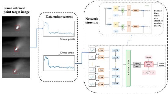
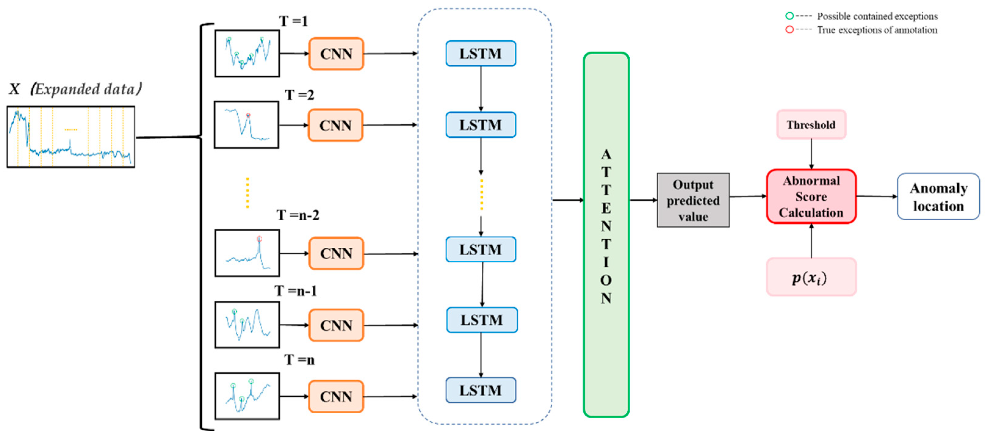
• A spatio-temporal hybrid network (CNN+LSTM) is designed for infrared target abnormal event sensing, called AC-LSTM, which focuses not only on the abnormal temporal characteristics of the target, but also on the spatial feature changes between the abnormal and normal states. It allows online real-time pre-processing and analysis of the target’s radiation characteristics and motion characteristics, instead of the traditional method that can only be processed afterward, to promptly observe and deal with the target during its flight. Moreover, compared with the traditional manual methods, our AC-LSTM has higher recognition accuracy and higher stability.
• A Periodic Time Series Data Attention (PTSA) module is proposed, which is incorporated into our AC-LSTM model with negligible overheads. It adaptively strengthens the “period” features to increase the representation power of the network by exploiting the inter-batch relationship of features. A large number of experimental results with real cases demonstrate that the PTSA module can help our AC-LSTM model better grasp the time-series data changes.
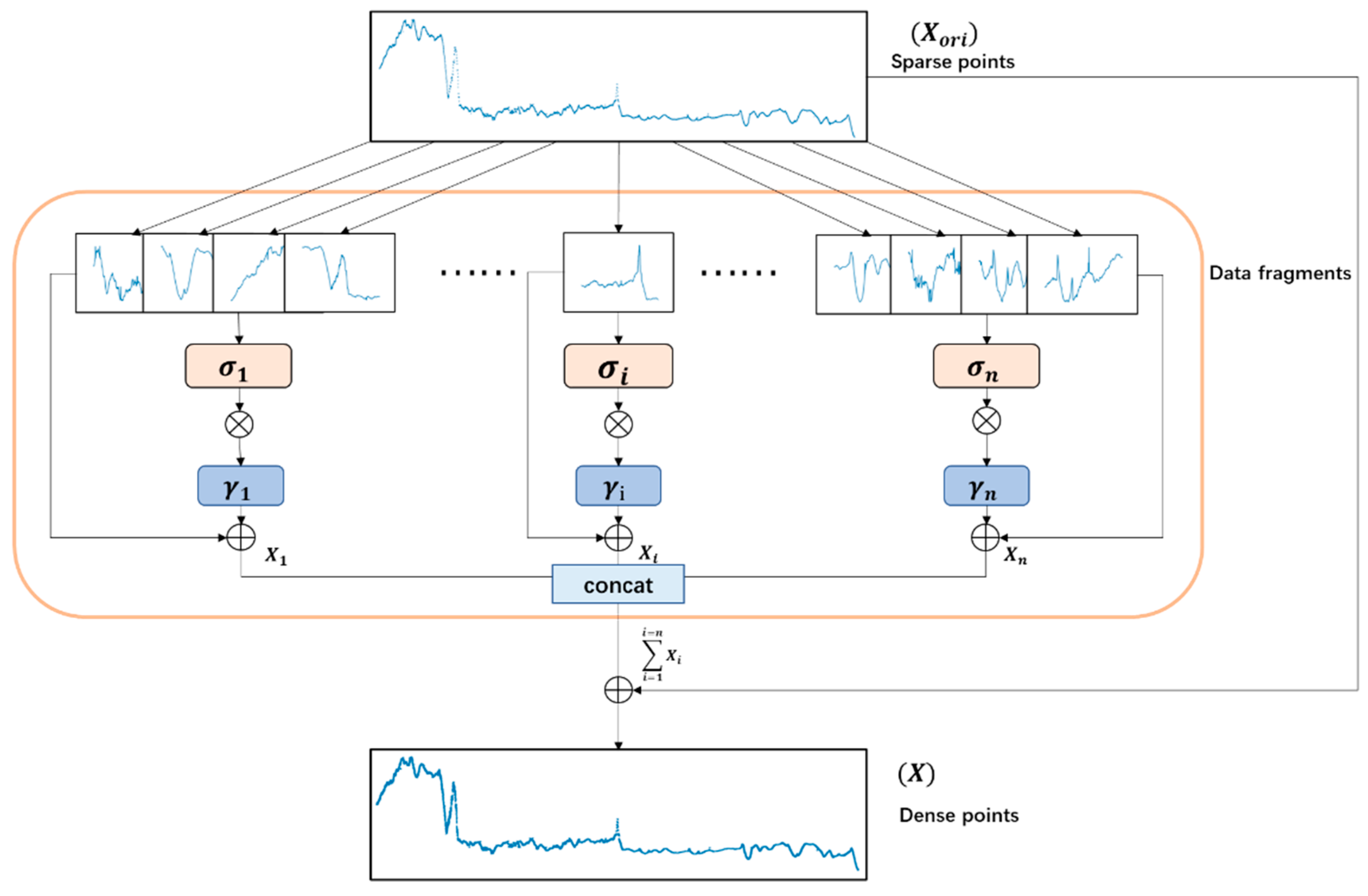
• A data expansion method is proposed to improve the generalization ability of our model. This method uses the time window method to expand a large number of data while keeping the overall trend of the target unchanged.

2. Related Work

Our work is inspired by the recent progress in time series anomaly detection in various fields. In this section, we describe related work for using the CNN+LSTM structure briefly.

2.1. Time Series Anomaly Detection Method

This “anomaly” is mostly defined as an irregularity in the data, as a deviation from the rules [7]. In the field of anomaly detection, Markov model-based approaches are widely used [8]. Markov models can predict future states using previous information. It can establish transfer probability relationships between states [9,10]. Gu et al. propose a stream-based mining algorithm combining Markov models and Bayesian classification methods, used for online anomaly prediction [11]. Their anomaly prediction scheme can alert impending system anomalies in advance and suggest possible causes of the anomalies. Sendi et al. [12] use Hidden Markov Models (HMM) to extract the interactions between the attacker and the network. Actually, machine learning-based anomaly detection is the adaptation of some data structures or classification models from machine learning to apply to anomaly detection tasks [13]. For example, Isolation Forest (IFF) uses a random hyperplane to cut the data space, where anomalous samples or outliers with sparse distribution density are more easily sliced into a subspace [14,15]. The One-Class Support Vector Machine (OCSVM) does not rely on density partitioning to find anomalies, by improving the support vector machine and using classification techniques for anomaly detection on time series data with extreme class imbalance [16,17,18]. Essentially, it converts binary classification into a single classification and marks the data as anomalous samples whenever they do not belong to the normal class. In recent years, deep learning methods based on neural networks have been widely used in prediction problems [19]. Recurrent neural networks (RNNs) and their advanced variants have shown higher performance than traditional methods in prediction tasks [20,21], capturing the features of input time series data by memorizing its historical information. Hochreiter et al. [22] propose LSTM units, a special type of RNN, to address the vanishing gradient problem that occurs in traditional RNNs, which results in the inability to learn long-term correlations. LSTMs introduce gating mechanisms to control the entire flow of information within a neuron, with both short-term and long-term dependencies. LSTM networks are particularly suitable for modeling multivariate time series and time-varying systems [23], and LSTM-based methods have demonstrated excellent anomaly detection capabilities. For example, Malhotra et al. [24] propose a stacked LSTM structure to detect anomalies in time series data. In contrast to the denoised LSTM, features without dimensionality reduction are used as input. Detection is achieved by assessing the bias of the predicted output based on analyses of variance. Bontemps et al. [25] present a method for detecting collective anomalies using LSTM. The novelty lies in evaluating the prediction error of multiple advance steps compared to evaluating each time step individually. The LSTM network improves the detection accuracy by modeling the prediction of smooth and non-smooth time correlations. As a result, efficient detection of temporal anomalous structures is achieved. Lee et al. [26] propose a real-time detection method implemented based on two LSTM networks. One is used to model short-term features and is capable of detecting individual upcoming anomalous data points within a time series, and the other is used for long-term threshold-based control detection.

2.2. Application of CNN+LSTM Algorithm

To implement multidimensional time series anomaly detection, convolutional neural networks (CNNs) and LSTMs are proposed to be combined, which allow anomaly detection in multiple and interconnected dimensions, such as spatial, temporal, or other application-specific dimensions [27,28,29]. In short, it is possible to detect complex anomalous structures by correlating different dimensions.

The combination of CNN, LSTM, and DNN is proposed in [6] to extract more complex features that can achieve anomaly detection of web traffic. Yao et al. [30] combine CNN and LSTM for traffic data prediction; this method proposes to combine the temporal dynamics and spatial dependence of traffic flow. Renjith et al. [31] use CNN+LSTM anomaly detection technique to detect suicidal ideation in social media platform posts, combining anomaly detection with user multidimensional thought logic. The same CNN+LSTM model is used in [32] for user evaluation, which can detect anomalies in text analysis to determine psychiatric categories. Convolutional neural networks are used to extract local information from text, and long- and short-term memory networks are used to extract contextual relevance. In [33], CNN-LSTM is used for multi-step wind power prediction, and CNN is used to extract spatially correlated feature vectors of meteorological elements at different sites and temporally correlated vectors of ultrashort-term meteorological elements, which are reconstructed by time series and used as input data for LSTM. Then, the LSTM extracts the temporal feature relationships between historical time points for multi-step wind power prediction. Rojas-Dueñas et al. [34] propose a method to detect the health status of electric vehicle power supply converters by training a CNN+LSTM model to predict the remaining service life of the device and the fault diagnosis of the device. In [35], a one-dimensional CNN+LSTM network structure is used for short-time traffic flow prediction, and the effectiveness of the algorithm is verified by conducting experiments on collected real data.

The above-related work verifies that CNN combined with LSTM can perform better anomaly detection than CNN-only or LSTM-only, but this method has not been applied for anomaly state perception of infrared point targets. As far as we know, our work is the first to apply anomaly detection to infrared point targets, which fills the gap in this field. Moreover, on the one hand, the target does not produce serious anomalies in most cases, and the abnormal state becomes missing compared to the normal state; on the other hand, different target characteristics have very obvious changes, and the data seriously lack periodicity. These bring higher requirements on the generalization and real-time analysis abilities of the algorithm.

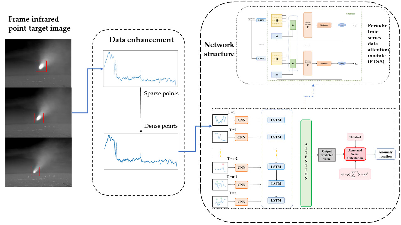
3. The Proposed Method

3.1. Data Enhancement

The infrared target feature data are closely linked with temporal information, and the temporal data of different targets will have great variability, resulting in a serious imbalance of data size. The high-dimensional input space corresponding to small samples is sparse, so it is difficult for neural networks to learn the mapping relationship from it. Data enhancement becomes an essential step in the process of network training. In order to enlarge the amount of data input and keep the length of the input data in the network consistent, the general data enhancement method will scale the input dataset to a certain length. This scaling is usually achieved by interpolation. However, this simple and basic method cannot increase the robustness of network learning, and it is easy to produce an over-fitting phenomenon in the training process. Inspired by [36,37], this paper proposes a sliding window slicing method to enhance data. This method can add random noise to the original data without changing the data distribution. The specific implementation process is shown in Figure 3.

${\mathit{X}}_{\mathit{o}\mathit{r}\mathit{i}}$ = (x₁, x₂, …, x_N) is the input vector of the target’s infrared characteristic data with length N, which is represented as sparse points in Figure 3. The original time series is sliced into data fragments ${\mathit{x}}_{\mathbf{1}}$ = ($x_1$, $x_2$, …, $x_n$) ${\mathit{x}}_{\mathbf{2}}$ = ($x_2$, $x_3$, …, $x_{n+1}$), ${\mathit{x}}_{\mathit{i}}$ = ($x_i$, $x_{i+1}$, …, $x_{i+n}$) according to a certain length $n$, where $x_i$ refers to the first frame of each sliced sequence. Here, $n$ can be set according to the total length of the sequence. In this paper, one slice is used every 500 frames. At the same time, each slice overlaps 100 frames of data of the previous slice. After splitting the original data slices, we calculate the average and standard deviation of each slice level.

$${\mu }_i=\frac{{\displaystyle \sum }{\mathit{x}}_{\mathit{i}}}{n}$$

(1)

$${\sigma }_i=\sqrt{\frac{{\displaystyle \sum }{({\mathit{x}}_{\mathit{i}}-{\mu }_i)}^2}{n}}$$

(2)

Generate a set of random arrays ${\mathit{\gamma }}_{\mathit{i}}$ according to the standard deviation of each slice data, where the length of ${\mathit{\gamma }}_{\mathit{i}}$ is the same as that of slice data. At the same time, the enhancement factor $b$ is set, which can be modified according to the situation. In this article, the default setting is 0.05. Multiply the random array with the standard deviation and add its result to the slice data. It is equivalent to generating a set of new data with the same data distribution as the slice data, but the data at each moment is randomly changed. The specific implementation procedure is shown in Equation (3), where vector ${\mathit{\sigma }}_{\mathit{i}}$ is the expansion of standard deviation ${\sigma }_i$ to the same dimension as ${\mathit{x}}_{\mathit{i}}$.

$${\mathit{X}}_{\mathit{i}}=b\ast {\mathit{\gamma }}_{\mathit{i}}\ast {\mathit{\sigma }}_{\mathit{i}}+{\mathit{x}}_{\mathit{i}}$$

(3)

$$\mathit{X}={\mathit{X}}_{ori}+{\displaystyle \sum }_{\mathit{i}=\mathbf{1}}^{\mathit{i}=\mathit{N}/\mathit{n}}{\mathit{X}}_{\mathit{i}}$$

(4)

The max data length is set to 100,000. In this way, the data are supplemented until the set data length is reached, and finally the enhanced data $\mathit{X}$ (dense points in Figure 3) is obtained. There are 4900 original data segments in the figure, which can reach 100,000 data points after data expansion. During training, all data will be sent to the network for testing, and the amount of data sent to the network will be the same every time.

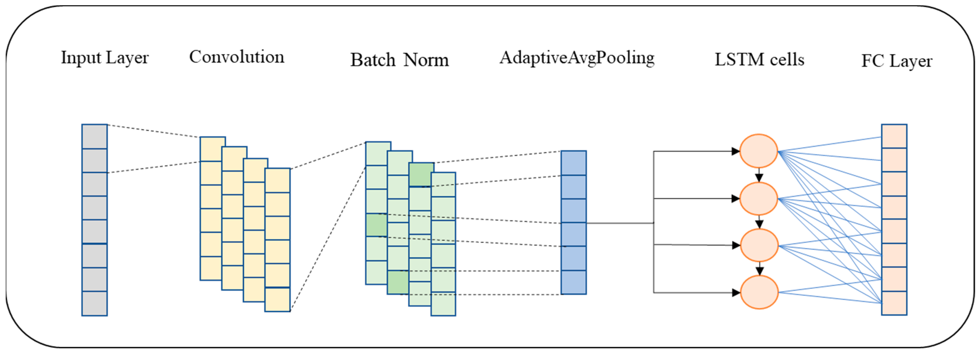
3.2. CNN-LSTM for Anomaly Detection

The CNN model is widely used in the field of feature engineering because of its focus on features. LSTM has the characteristics of time series expansion and is widely used in time series. The anomaly detection in this paper is a kind of spatial feature extraction which is highly correlated with time series. Therefore, this paper combines two structures for anomaly detection of infrared point targets. Inspired by state-of-the-art CNN+LSTM algorithms [6,38,39], we propose the AC-LSTM network, which consists of CNN and LSTM layers, and PTSA module with the self-attention mechanism (this part will be described in Section 3.3) [40]. Its structure is shown in Figure 4. The network uses fixed-length time series data as input. The time series has been greatly expanded by the data enhancement module, and the amount of data is dozens of times larger than the original data. The spatial elements of the abnormal part of the input data are extracted by the CNN network, and the time characteristics of the data are extracted by LSTM. Then, the anomaly score of each point after single-step prediction is calculated, and the anomaly location is judged by adaptive threshold determination, and then fed back to the temporal data to obtain the specific moment when the anomaly occurred in the process of target flighting.

The first part of our network adopts CNN structure. Figure 5 shows the specific structure of the network, which is mainly composed of the Convolution layer, Batch Norm (BN) layer, Pooling layer, and Full Connection (FC) layer. Before starting the training, the time series data with a fixed length of M (the max data length mentioned in Section 3.1) are divided into a small data window containing m data according to batch_size, which is expressed as $\mathit{X}=\left(x_1,x_2,\dots ,x_m\right)$. Subscript m represents the size of the batch. $\mathit{X}$ is taken as input and sent into the convolution layer. After that, the data in each window pass through the convolution layer, and the spatial features of each part of the data can be extracted. Sending the feature map to the BN layer for normalization can accelerate the convergence speed of the network and prevent the gradient explosion. Then, the data are processed by activating the function to complete the data. The specific implementation process is expressed in Equation (5). $x_i$ represents each value in the output feature map, where $i$ is the index of the characteristic value. $y_i{}^T$ represents the output value of t time step, $W_i$ is the corresponding weight coefficient, $\sigma$ is the activation function, which can be tanh or relu. We also add a dropout layer to the first convolution layer, which can effectively prevent the data from over-fitting. It should be noted that in this process, each slice window is fed into the convolutional neural network in a sequential manner. In this paper, the pooling layer adopts adaptive average pooling of Pytorch, which will control the output size according to the input parameters. The pooling layer can effectively reduce the size of the parameter matrix, thus reducing the number of parameters in the final connection layer. Therefore, adding pooling layer can speed up the calculation and prevent over-fitting.

$$y_i{}^T=\sigma (b_i+{\displaystyle \sum }_{i=1}^m{W}_i{x}_i)$$

(5)

The second part of our network adopts LSTM structure. CNN acquires complex spatial features of the input signal. After that, the feature vector of each data window is sent into LSTM. $W_T$ which in Equation (6) represents the total weight coefficient of the CNN, $y_i{}^T$ is the output feature vector of the CNN at each time step, $F_T$ represents the output of each time step through the LSTM cell, and $F$ represents the process of the feature vector through the LSTM.

$$F_T=F\left(W_T\ast y_i{}^T\right)$$

(6)

The LSTM in Figure 4 is a repeatable stacked unit. These units acquire the temporal characteristics of data in different time steps T through continuous learning. The process mainly includes three different gate structures: forgetting gate, memory gate, and output gate. These three gates are used to control the information retention and transmission in the long- and short-term memory network, which can be expressed as follows [3].

• Forgetting phase. The forgetting gate $f_t$ consists of a Sigmoid neural network layer and a per-bit multiplication operation. The $h_{t-1}$ in Equation (7) is previous hidden layer status. The $x_t$ is the input of data. The $b_f$ is offset value. The $\sigma$ represents the Sigmoid function.

$$f_t=\sigma \left(W_f·\left[h_{t-1},x_t\right]+b_f\right)$$

(7)

• Selective memory stage. The role of the memory gate is the opposite of the forgetting gate, which will determine among the newly entered information $x_t$ and $h_{t-1}$, what of the information will be retained. The $\widetilde{C_t}$ in Equation (9) is the out-of-selective memory stage.

$$i_t=\sigma \left(W_i·\left[h_{t-1},x_t\right]+b_i\right)$$

(8)

$$\widetilde{C_t}=i_t\ast \tanh \left(W_c·\left[h_{t-1},x_t\right]+b_c\right)$$

(9)

The results obtained from the above two steps are added together to obtain the $C_t$.

• Output phase. This phase will determine what will be treated as the output of the current state. Then, at the $t$ time, we input the signal $x_t$. Later, the corresponding output signals are calculated according to Equations (10) and (11).

$$o_t=\sigma \left(W_o\left[h_{t-1},x_t\right]+b_o\right)$$

(10)

$$h_t=o_t\ast \tanh \left(C_t\right)$$

(11)

The cell output cells of different time steps are concurrently connected, and the purpose of this step is to learn the anomalous part with fewer data and finer details when the feature map goes through several time steps of the LSTM. The output of the first LSTM layer is passed as input to the second layer. This is also capable of temporally associating data from each time period over a long period of time, which is equivalent to temporally associating the entire data with strong data. The CNN is equivalent to narrowing down a certain retrieval range for the input of the LSTM, while the LSTM is still able to perform internal temporal data prediction within each small time segment to obtain the anomalies of the data within each time segment.

The red part in Figure 4 is the last part. It performs the anomaly location determination. Calculate the mean value ${\mu }_t$ and standard deviation ${\sigma }_t{}^2$ for each region $x_t$. For each anomaly point, $x_i$ can be computed as an anomaly score $p\left(x_i\right)$.

$$p\left(x_i\right)={\displaystyle \prod }_{i=1}^{i=t}\frac{1}{\sqrt{2\pi }{\sigma }_i}\exp (-\frac{{\left(x_i-{\mu }_i\right)}^2}{2{\sigma }_i^2})$$

(12)

As the target exception needs to continue online judgment, set the judgment threshold $\epsilon$. Threshold value $\epsilon$ is set using the local average method, and the data are calculated in a stepwise flow. The ${\mu }_T$ which is the average of the abnormal scores is calculated within each time step T. Order $\epsilon ={\mu }_T$, If $p\left(x_i\right){\displaystyle >}\epsilon$, then this place is identified as an abnormal point, and the timing data are combined with locking the abnormal frame and filtering out the final abnormal location.

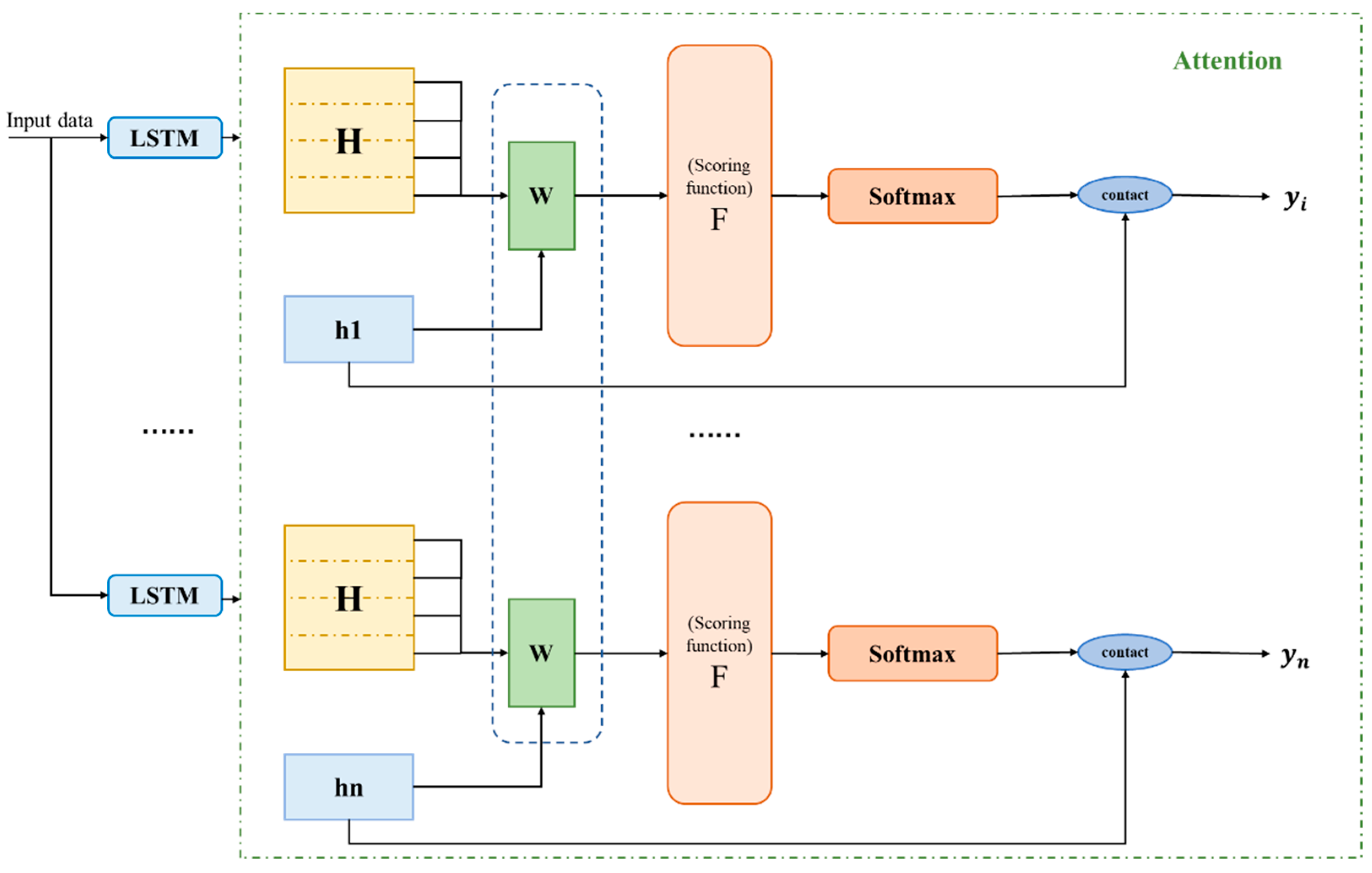
3.3. Periodic Time Series Data Attention

The attention mechanism [41] has demonstrated excellent performance in 2D image feature extraction in recent years, thus we try to use it in 1D time series data that propose the periodic time series data attention (PTSA) module. Unlike two-dimensional image data, our one-dimensional input data have a very strong temporal correlation. Although they still need to be split into many batches for training, there is a very tight connection between each batch. This requires that our attention model cannot focus only on the features of each part. Inspired by [42,43], our proposed PTSA module is able to combine the data features of each batch periodically. The implementation process is mainly shown in Figure 6. The attention mechanism is mainly to judge the importance of each input by weighting. Within each batch, we still adopt the simplest one-dimensional data attention method. The working principle of the LSTM encoder-decoder integrated with the attention mechanism can be expressed by the following equations. The hidden state of the current LSTM unit in the LSTM encoder is H, and the hidden state of the first LSTM unit in the LSTM decoder is h₁. First of all, it is necessary to score the degree of correlation.

$$Score=F\left(H,h_1\right)$$

(13)

In this paper, the F function used in scoring is the bilinear function, where $W$ is the weight matrix that can be learned.

$$F\left(H,h1\right)=H^{T}W{h}_1$$

(14)

Next, the attention weighted distribution matrix $\mathit{a}=\left(a_1,a_2,a_3,\dots ,a_m\right)$ is generated by the softmax function, where each item corresponds to the input, where $h_i$ is the hidden state of the ith LSTM unit.

Finally, these attention distributions can selectively extract relevant information from the input information. The final attention weighting matrix is linked with the hidden layer unit of LSTM, and the final output prediction value is obtained. Our proposed periodic attention mechanism realizes weight sharing among each LSTM unit to realize the final network prediction jointly.

$$y_i=a_i\ast h_i$$

(15)

4. Experiment

4.1. Experimental Setup

4.1.1. Training Details

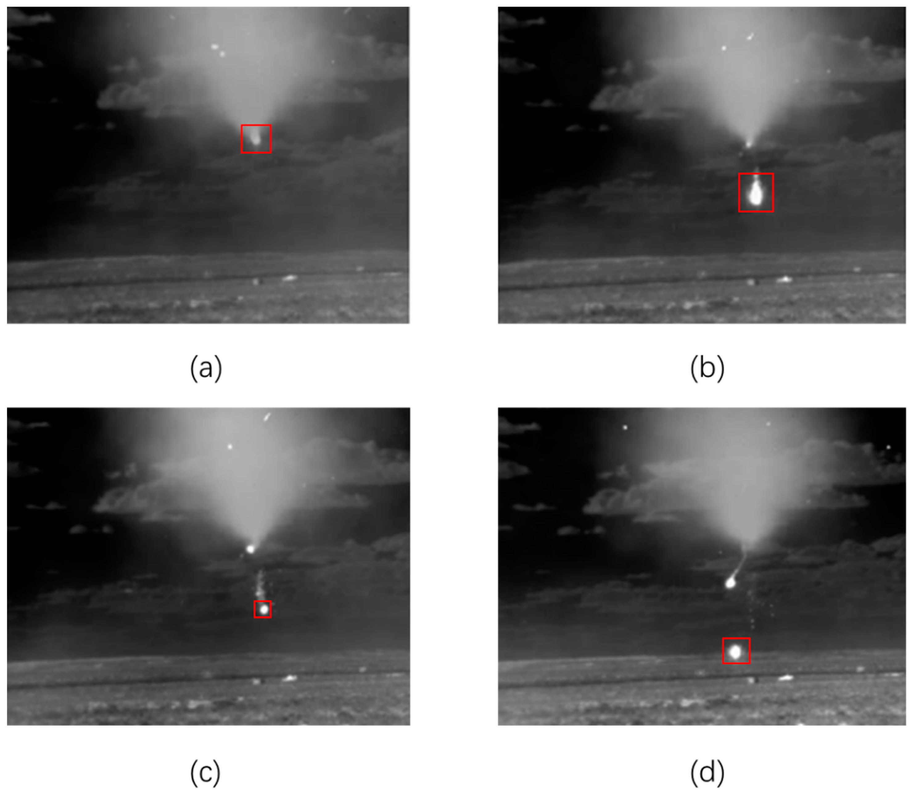
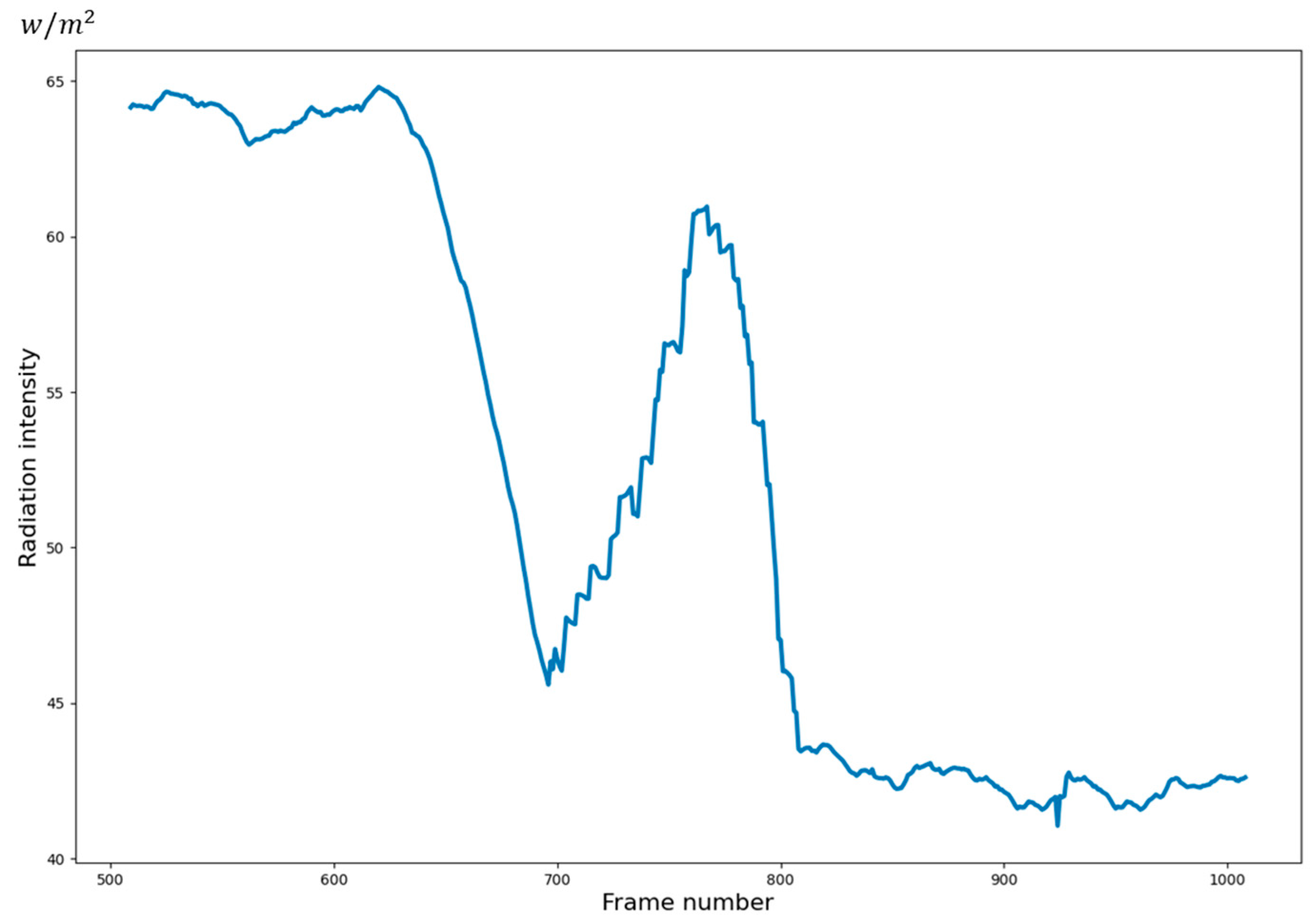
Since the experimental network model deals with one-dimensional time series data variables, it does not require a very powerful hardware configuration (it takes about 10s to run an epoch using a single GeForce RTX 2080ti GPU). The problem of data latency is unavoidable when using LSTM for temporal data prediction due to the fact that the predicted values produce very large deviations in the first prediction to keep the same size as the original data. Thus, many works use the mean or median of the data instead of the first prediction, but this will also lead to the anomaly scores of the first frame tending to be very high. This problem is exacerbated by the fact that our dataset has very large data variations. Therefore, we avoid this problem by adding a start point and an endpoint to the prediction and calculation of the anomaly scores.

4.1.2. Datasets

The datasets we use are all real infrared images obtained in our work accumulation, which are the continuous frames of data captured during the motion of the flying target, and it contains roughly 30 groups, each group containing 3000–8000 frames, and the anomalous frames are manually marked by experts to be used to analyze and label the target anomalous events. Figure 7 shows some of our data. The red box is where the abnormal event occurs. The curve in the figure is the effect of drawing one-dimensional time series data. In fact, the data we send into the network are data of a certain length, abnormal data are marked as 1, and normal data are marked as 0. Although the data volume is very large, the number of anomalous frames is still very small in the total data volume. That led to our dataset of anomaly detection being not as easy to obtain as car traffic monitoring and various machine fault detection, thus we use a sliding window slicing method to enhance our dataset (introduced in Section 3.1).

4.1.3. Evaluation Metric

We use the evaluation metrics Precision, Recall, Accuracy, and F1 score that are commonly used in anomaly detection to determine the effectiveness of our proposed method [44].

TP (True Positive): Abnormal point is predicted to be abnormal.

FP (False Positive): Normal points are predicted to be abnormal.

FN (False Negative): Abnormal point is predicted to be normal.

TN (True Negative): Normal point is predicted to be normal.

TP, TN, FP, and FN rates are used to evaluate each algorithm in our experiment.

$$precision=\frac{TP}{TP+FP}$$

(16)

$$recall=\frac{TP}{TP+FN}$$

(17)

$$accuracy=\frac{TP+TN}{TP+TN+FN+FP}$$

(18)

Precision in Equation (16) is the percentage of relevant instances among all retrieved instances and recall in Equation (17) is the percentage of relevant instances retrieved among all relevant instances. Accuracy in Equation (18) is the proportion of the whole sample that is judged correctly. The recall is a particularly important metric for anomaly detection because it represents the ratio of the number of anomalies found to the total number of anomalous instances.

$$F1Score=2\times \frac{precision\times recall}{precision+recall}$$

(19)

Using precision and recall, we can derive F1 scores, as shown in Equation (19). We used these evaluation metrics to make a quantitative comparison of the test results.

4.2. Ablation Studies

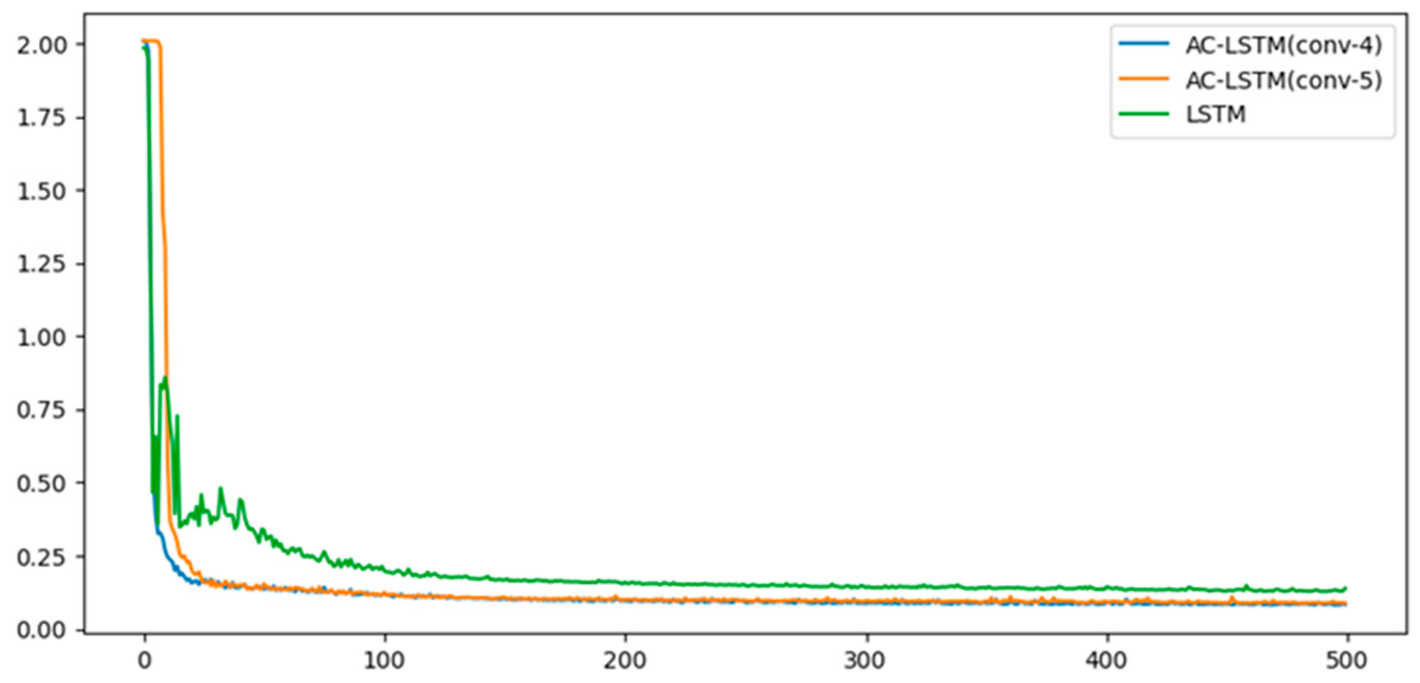
4.2.1. Performance Comparison of Model Combinations

We verify the performance of our network model by combining different structures. Our benchmark method is LSTM single-step prediction [45]. On this basis, we add different convolution layers and change the network structure. In fact, using LSTM or CNN alone for anomaly detection of infrared point targets is not satisfactory. The LSTM prediction method (the first row of

Table 1. Performance comparison of different model combinations.

Method		Precision	Recall	F1-Score
LSTM		0.27	0.9	0.41
CNN		0.63	0.8	0.27
LSTM+CNN	Conv(3)	0.77	1.0	0.36
	Conv(3) + BN(3)	0.82	1.0	0.47
	Conv(4) + BN(4)	0.83	1.0	0.47
	Conv(5) + BN(5)	0.83	1.0	0.47

) has very low precision, although its F1 Score is higher than that of CNN. A large number of false alarms will be generated when an abnormal event occurs, which is an excessive reminder for the early warning work and will consume a lot of labor costs to maintain. The CNN method (the second row of Table 1) performs worst on all indicators. Our AC-LSTM adds a one-dimensional convolution layer to LSTM to help the network get more information, and the effect is significantly higher than that of the two models alone. The second half of the table shows the test of our model by changing the number of convolution layers. The accuracy has been obviously improved by adding three convolution layers. This result confirms our previous point of view that joining CNN can obtain more spatial characteristics of data based on the original network structure. On this basis, we added a Batch Normalization (BN) layer [46] after each convolution layer and found that the effect was obviously improved. However, with the deepening of network layers, the experimental results were not improved again. This phenomenon may be due to the simple structure of time series data, and even the complex model has a limited ability to extract features from one-dimensional data.

4.2.2. Effect of Sliding Window Enhancement

In

Table 2. The effect of different enhancement methods. (Long-term noise refers to the enhancement of all data once in the way of interpolation instead of window slicing, and segmented noise refers to the enhancement method of sliding window proposed in this paper.).

	Precision	Recall	F1-Score
AC-LSTM	0.53	0.8	0.37
AC-LSTM+Long-term noise	0.75	1.0	0.42
AC-LSTM+Segmented noise	0.83	1.0	0.47

, we evaluate the effect of our data expansion method (introduced in Section 3.1). We take AC-LSTM, which uses the original data as input, as the basic network, comparing it with ones adding long-term noise and segmented noise. The results show that adding noise to our input data can effectively improve the generalization ability of our model, especially adding segmented noise by our proposed sliding window brings more significant performance improvement (the third row of Table 2). The input data used in the other experiments are all processed through our expansion method.

4.2.3. Effect of Periodic Time Series Data Attention (PTSA) Module

To thoroughly evaluate the effectiveness of our proposed PTSA (see Section 3.3), we take AC-LSTM without any attention module as the basic network. In the second row of

Table 3. The effect of attention module.

Method	Precision	Recall	F1-Score
AC-LSTM	0.83	1.0	0.47
AC-LSTM+Attention	0.83	1.0	0.47
AC-LSTM+PTSA	0.84	1.0	0.49

, we add a basic attention module of one-dimensional time series data to judge the importance of elements by encoding and decoding. However, it hardly brings increases or decreases to three indicators, which can be attributed to the fact that conventional attention modules are ineffective for anomaly detection. In the third row of Table 3, we add our periodic attention model (PTSA) to the basic network, bringing better performance on three indicators. It validates our assumption that data pays great attention to time series, and the periodic attention model can closely combine the data of each batch, which improves the correlation degree of data in time.

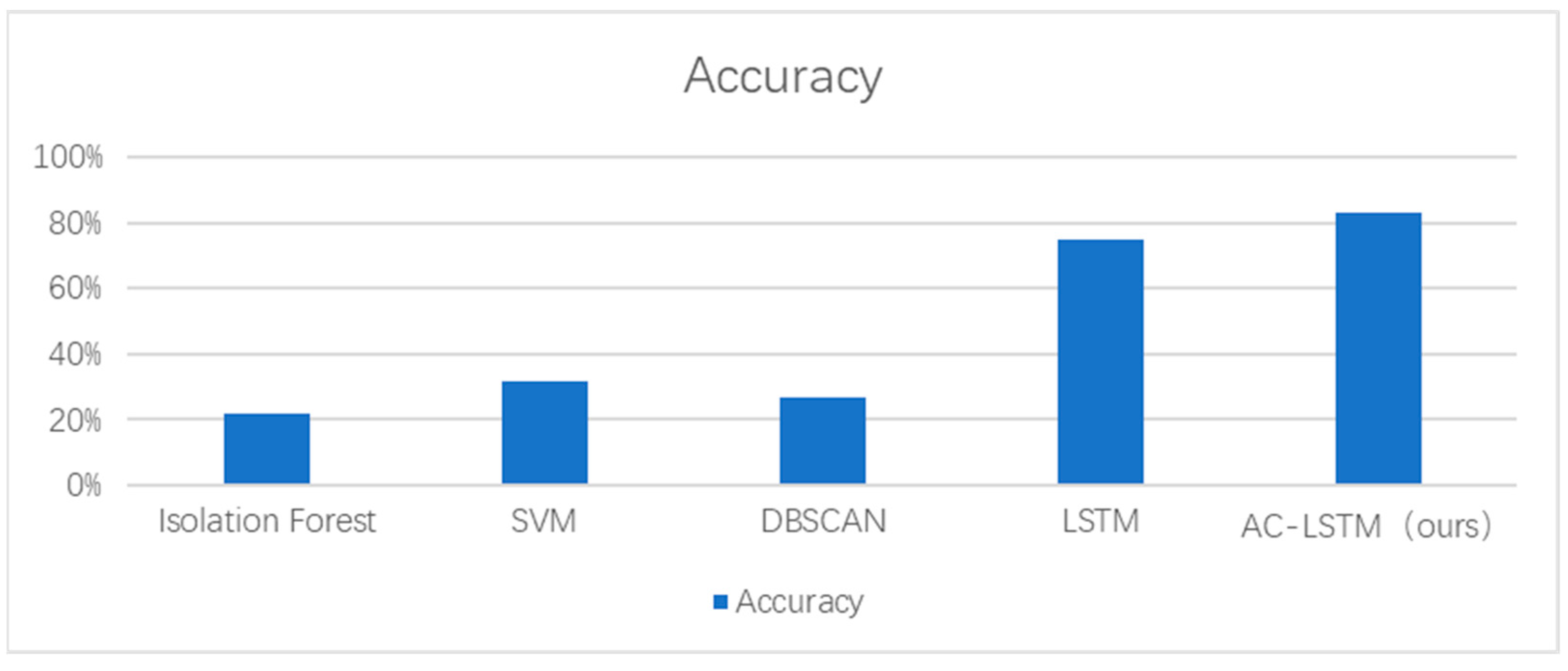
4.3. Comparison with State-of-the-Art Methods

In this section, we evaluate our implementation, which refers to AC-LSTM containing sliding window enhancement, CNN-LSTM layers, and periodic time series data attention modules (introduced in Section 3). We compare ours with several classical anomaly detection algorithms as comparisons including the Isolated Forest algorithm [14], the KNN algorithm [47], and the DBSCAN clustering algorithm [48], using the same data and parameters setup. Figure 8 demonstrates that our method far outperforms current classical algorithms in terms of accuracy. We believe that this is because these classical methods using clustering are always applied to isolated anomalies (as shown in Figure 9), but our infrared point targets are a rapid change when anomalies occur, the so-called isolated points do not easily exist due to the very dense shooting frames. As far as we know, there are fewer current machine learning methods published for anomaly state perception of infrared point targets (our proposed method fills in the gaps). Hence, we just compare LSTM [24] (a stacked LSTM structure to detect anomalies in time series data) with ours (in Table 1), and our scores significantly outperform it, which proves that our network has a powerful and robust learning ability to grasp nuances of different changes from limited samples.

4.4. Qualitative Analysis

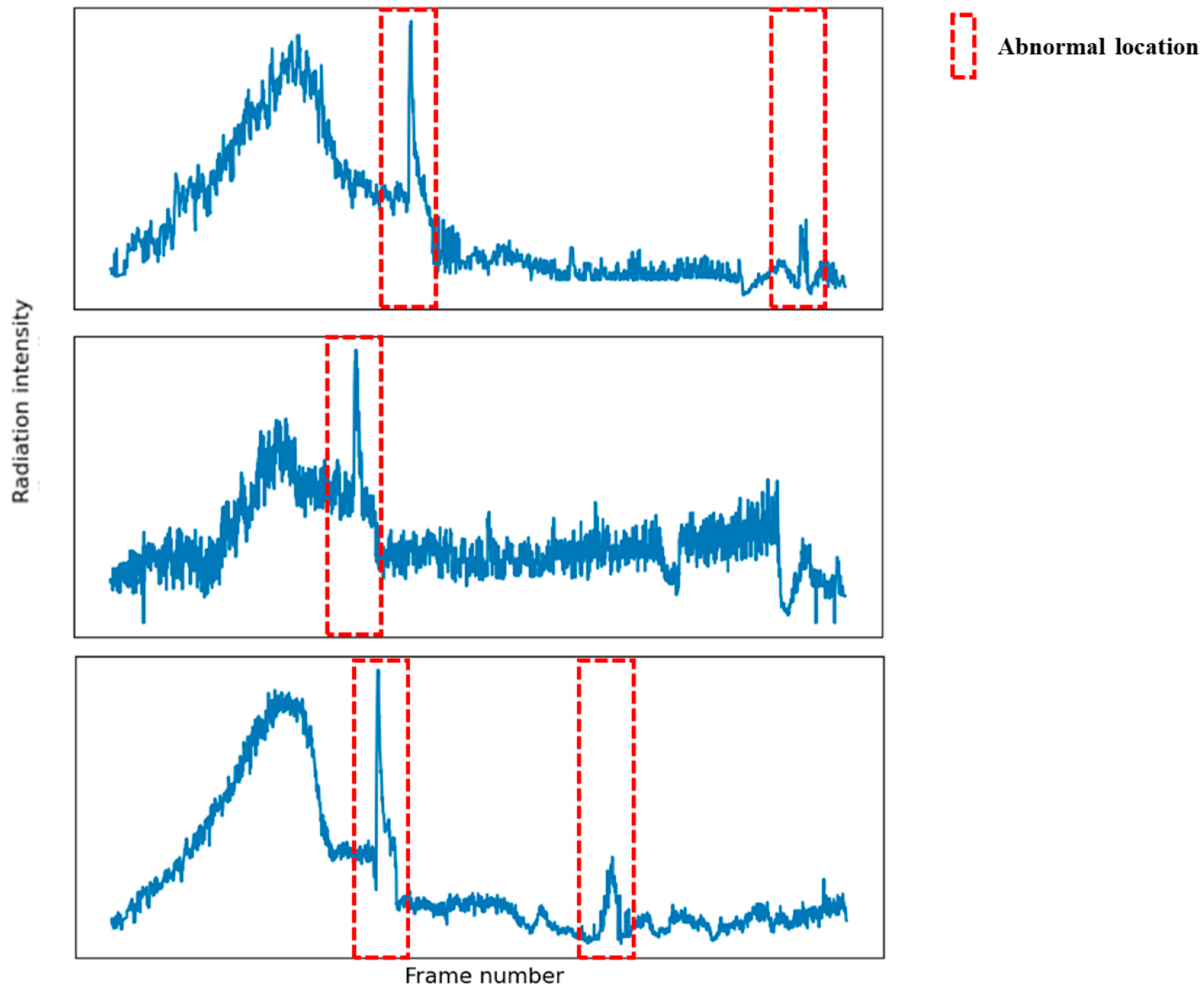
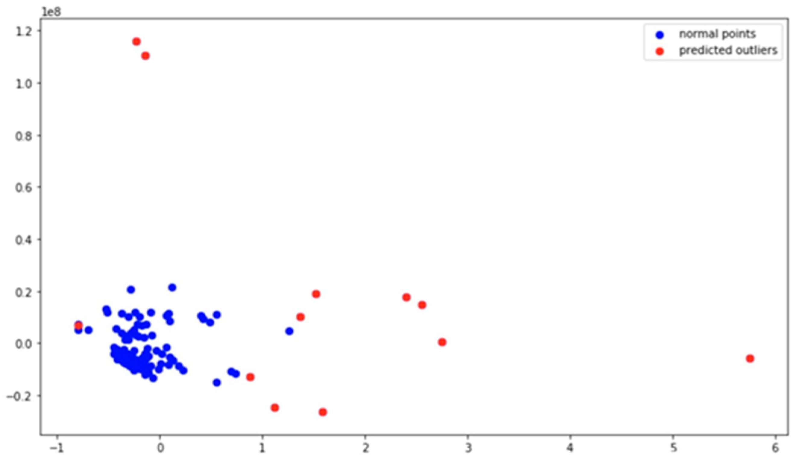
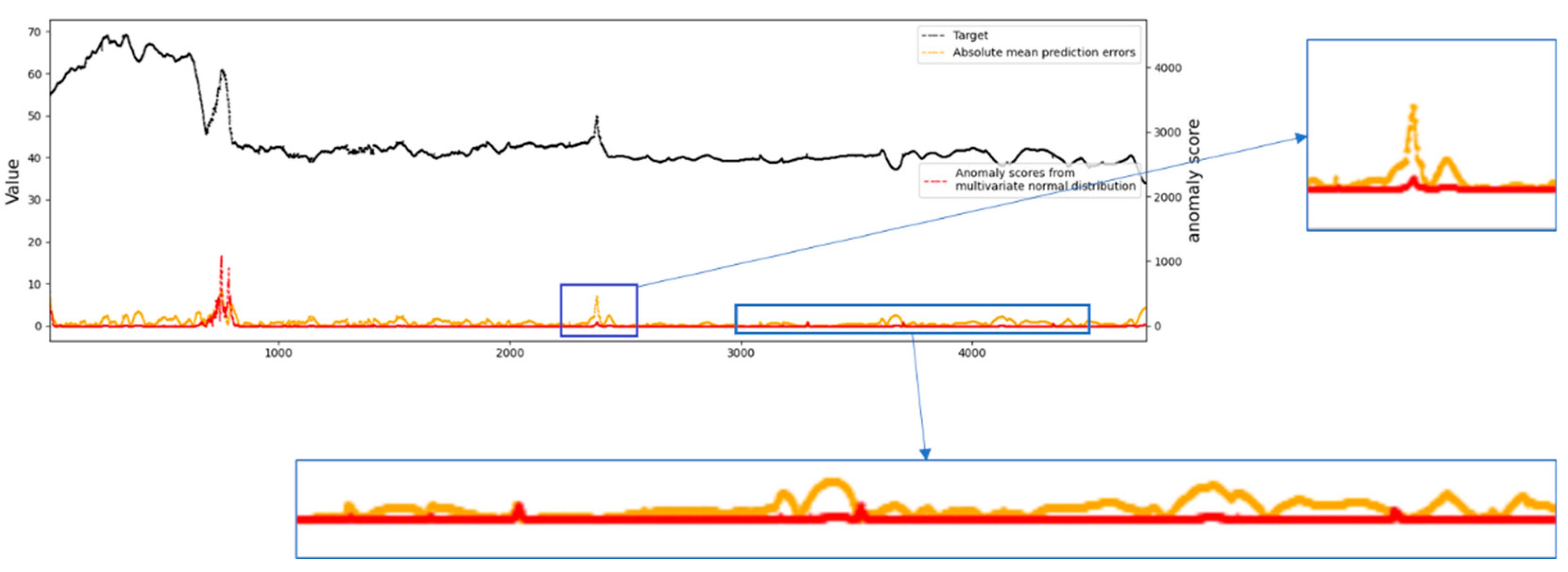
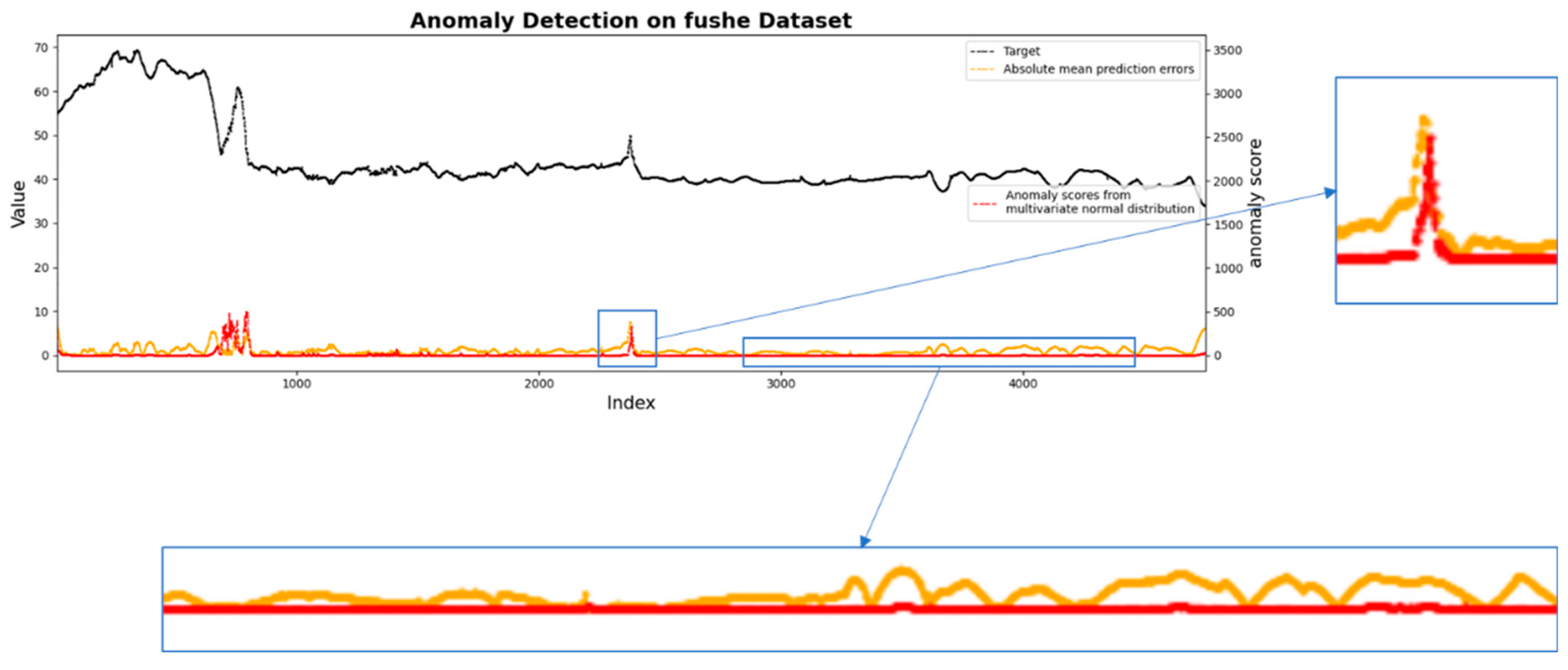
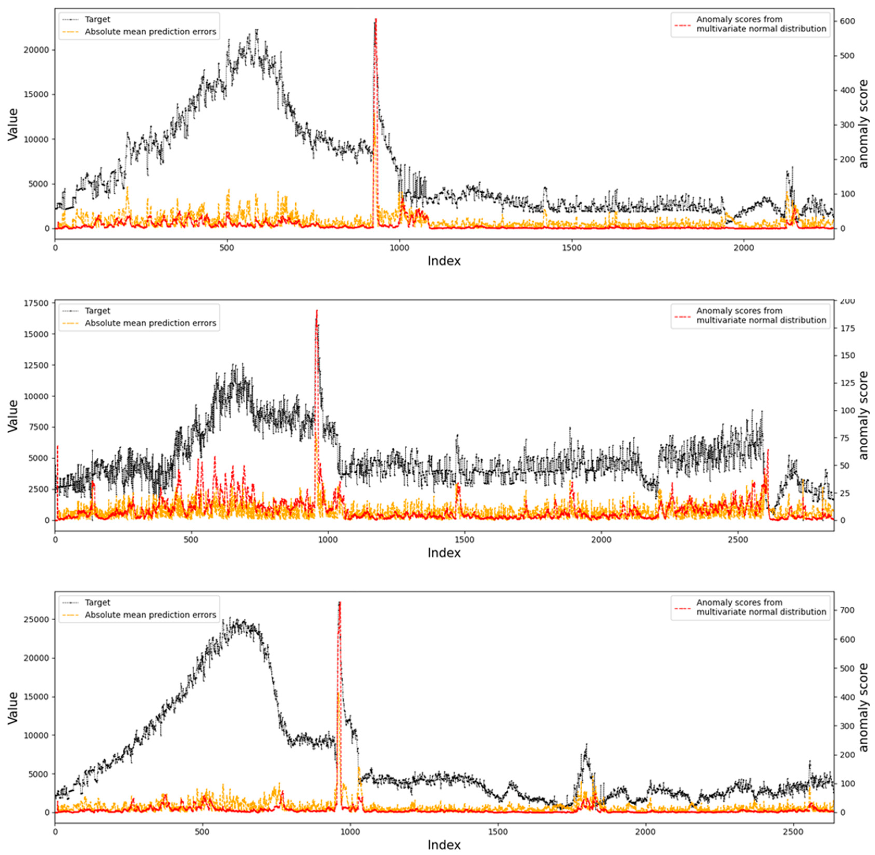
4.4.1. Visualization of Anomaly Detection Results

From Figure 10 and Figure 11, it can be clearly seen that LSTM-only performs reasonably effectively when the first abnormal event occurs, but it accumulates errors in long-term prediction, resulting in poor performance of the second abnormal event (not as good as the classical absolute mean prediction error score), although the abnormal scores of some non-abnormal areas can be kept low by learning. Notably, our model can perfectly detect these two kinds of abnormal events and the abnormal score can be kept very low in the non-abnormal area. As can be seen from the figures, although using LSTM-only has a higher abnormal score than our model when the first abnormal event occurs, it is not good for the later threshold judgment. This situation will correspondingly raise the threshold of the abnormal score, resulting in the second abnormal being completely discarded. On the whole, the performance of our model is better than that of using LSTM-only for anomaly detection. Figure 12 shows the effect of LSTM-only and our AC-LSTM on various indicators. It is obviously superior to LSTM-only in Accuracy, Recall, and overall F1 Score index, and the accuracy and recall can keep a good balance. It further validates that our model is obviously better than that of using LSTM-only for anomaly detection.

Figure 13 shows other detection results on our datasets. It can be seen that our methods can clearly detect the abnormal position and the abnormal score is much higher than that of the non-abnormal area.

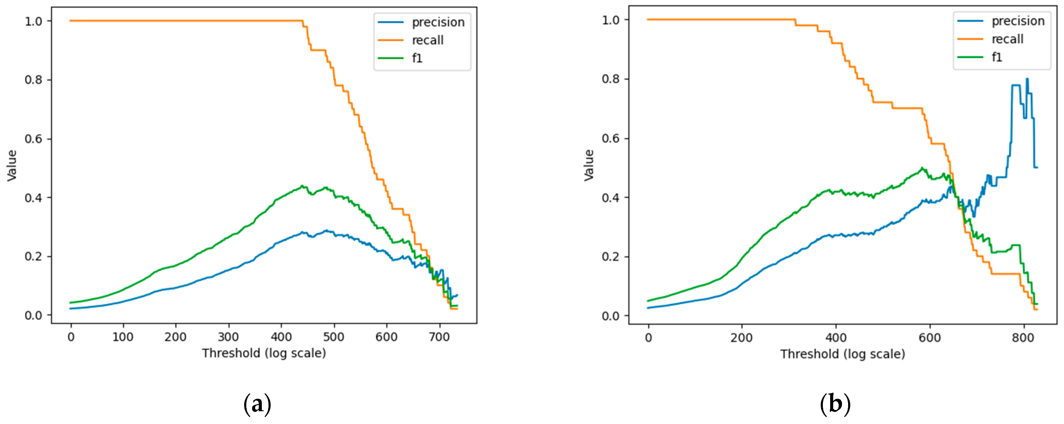
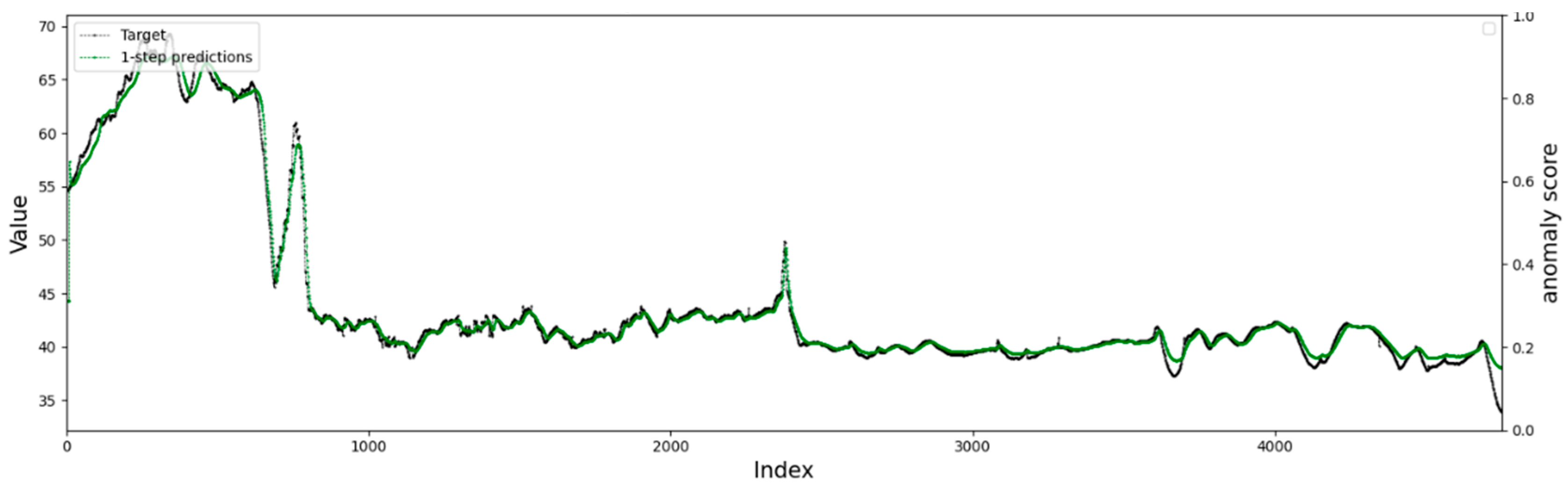
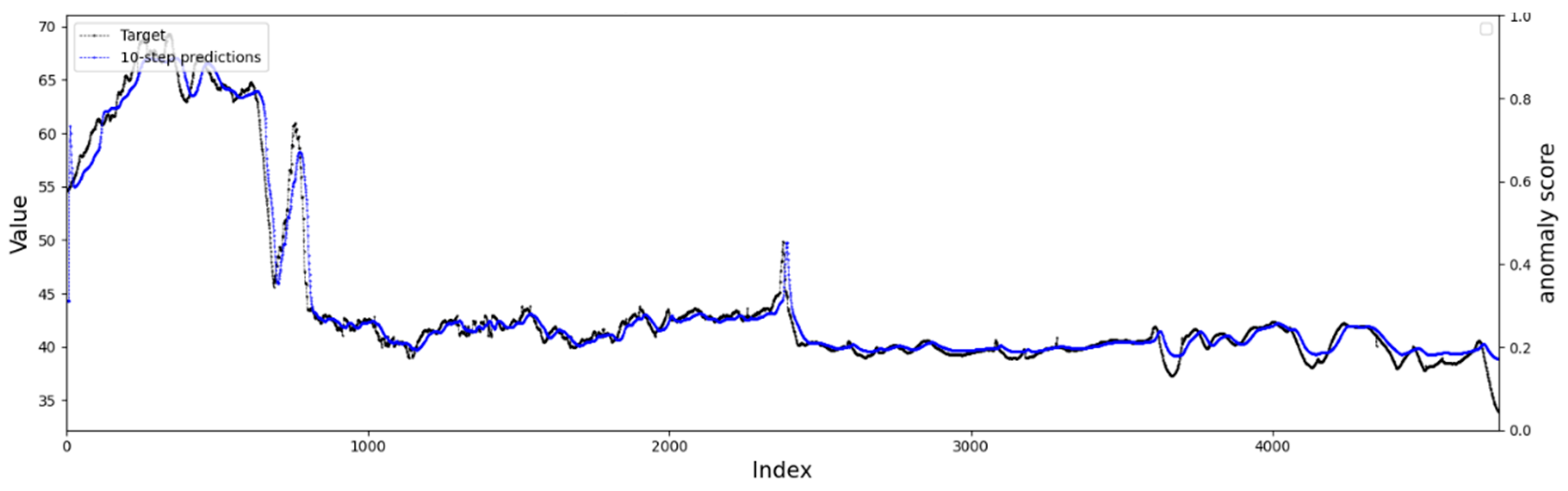
4.4.2. Comparison of Single-Step and Multi-Step Prediction Results

The data we use are time series data sampled at equal intervals. For such data, our “single-step prediction” means that an input data sequence is a complete event containing unusual moments. “Multi-step prediction” means that the intermediate results of predicting are used in the predicting process, resulting in an accumulation of errors. However, in scenarios that require real-time anomaly detection and early warning, the estimation of future values by multi-step prediction is very important. As can be seen from Figure 14 and Figure 15, when our network adopts multi-step prediction, although the general data trend can be learned, the detailed prediction of the data is not good and needs to be further strengthened.

4.5. Error Analysis

Figure 16 shows the cross-entropy loss function curves for LSTM and AC-LSTM with different convolution layers. It is intuitive to see that our proposed model has the lowest cross-entropy versus only using LSTM. Moreover, our model is relatively stable, and there is no big fluctuation. When four convolution layers are added, the model reaches the best, and adding more convolution layers will slow down the convergence rate. This experimental phenomenon is the result of network structure and experimental data. The network structure is too complex, the training is more difficult, and it is not suitable for our data volume, which may lead to our training embedding being locally optimal, making it difficult to get better results, or even degrading to a certain extent.

5. Conclusions

In this paper, we propose a new algorithm model AC-LSTM for anomaly detection of infrared point targets. As far as we know, this is a brand-new application scenario in the field of anomaly detection and has very important practical application value. In our work, many classical methods are applied to the anomaly perception of infrared point targets and compared with our proposed methods. We have explored many algorithms for anomaly detection based on intelligent methods (mainly LSTM-based predictive learning methods). On this basis, we have improved our algorithm, mainly including (1) adding convolution layers in the network to abstract more comprehensive data features, (2) proposing the periodic time series attention module, and (3) expanding input data through the sliding window in preprocessing stage. In the ablation experiment, it was confirmed that the modules we added can be improved on the baseline, each module has played a role, and relatively optimal results have been obtained. Through a large number of qualitative experiments, we find that our algorithm keeps a low abnormal score for non-abnormal data, and the algorithm as a whole has better performance and a more robust abnormal score.

However, there are still many shortcomings in our algorithm, so we cannot make leap-forward progress in F1 Score, and the multi-step prediction results are not so perfect due to the accumulation of errors. Moreover, the infrared point target will face numerous special situations in real situations, and our dataset cannot cover all the abnormal situations, which is why we will continue to accumulate and improve the algorithm in the future.

References

1. Yamazaki, S. Investigation on the usefulness of the infrared image for measuring the temperature developed by transducer. Ultrasound Med. Biol. 2008, 35, 1698–1701. [Google Scholar]
2. Wang, P. Research on Infrared Target Detection and Tracking Technology in Complex Background with Large Field of View; National University of Defense Technology: Changsha, China, 2018. [Google Scholar]
3. Gf, A.; Schmidhuber, J.; Cummins, F. Learning to Forget: Continual Prediction with LSTM. In Proceedings of the Istituto Dalle Molle di Studi Sull Intelligenza Artificiale, Lugano, Switzerland, 15 August 1999. [Google Scholar]
4. Loganathan, G.; Samarabandu, J.; Wang, X. Sequence to Sequence Pattern Learning Algorithm for Real-Time Anomaly Detection in Network Traffic. In Proceedings of the 2018 IEEE Canadian Conference on Electrical & Computer Engineering, Quebec, QC, Canada, 13–16 May 2018; pp. 1–4. [Google Scholar]
5. Zenati, H.; Foo, C.S.; Lecouat, B.; Manek, G.; Chandrasekhar, V.R. Efficient GAN-Based Anomaly Detection. arXiv 2018, arXiv:1802.06222. [Google Scholar]
6. Kim, T.Y.; Cho, S.B. Web Traffic Anomaly Detection using C-LSTM Neural Networks. Expert Syst. Appl. 2018, 106, 66–76. [Google Scholar] [CrossRef]
7. Ullah, W.; Ullah, A.; Haq, I.U.; Muhammad, K.; Baik, S.W. CNN Features with Bi-Directional LSTM for Real-Time Anomaly Detection in Surveillance Networks. Multimed. Tools Appl. 2020, 80, 16979–16995. [Google Scholar] [CrossRef]
8. Tan, X.; Xi, H. Hidden semi-Markov model for anomaly detection. Appl. Math. Comput. 2008, 205, 562–567. [Google Scholar] [CrossRef]
9. Tan, Y.; Hu, C.; Zhang, K.; Zheng, K.; Davis, E.A.; Park, J.S. LSTM-based Anomaly Detection for Non-linear Dynamical System. IEEE Access 2020, 8, 103301–103308. [Google Scholar] [CrossRef]
10. Xia, Y.; Li, J.; Li, Y. An Anomaly Detection System Based on Hide Markov Model for MANET. In Proceedings of the 2010 6th International Conference on Wireless Communications Networking and Mobile Computing (WiCOM), Chengdu, China, 23–25 September 2010. [Google Scholar]
11. Gu, X.; Wang, H. Online anomaly prediction for robust cluster systems. In Proceedings of the 2009 IEEE 25th International Conference on Data Engineering, Shanghai, China, 29 March–2 April 2009; pp. 1000–1011. [Google Scholar]
12. Sendi, A.S.; Dagenais, M.; Jabbarifar, M.; Couture, M. Real Time Intrusion Prediction based on Optimized Alerts with Hidden Markov Model. J. Netw. 2012, 7, 311. [Google Scholar]
13. Kaur, H.; Singh, G.; Minhas, J. A Review of Machine Learning based Anomaly Detection Techniques. arXiv 2013, arXiv:1307.7286. [Google Scholar] [CrossRef]
14. Fei, T.L.; Kai, M.T.; Zhou, Z.H. Isolation Forest. In Proceedings of the IEEE International Conference on Data Mining, Washington, DC, USA, 15–19 December 2008. [Google Scholar]
15. Liu, F.T.; Ting, K.M.; Zhou, Z.H. Isolation-Based Anomaly Detection. ACM Trans. Knowl. Discov. Data 2012, 6, 1–39. [Google Scholar] [CrossRef]
16. Olkopf, B.S.; Williamson, R.; Smola, A.; Shawe-Taylor, J.; Platt, J. Support Vector Method for Novelty Detection. In Proceedings of the Advances in Neural Information Processing Systems, Denver, CO, USA, 11 May 2000. [Google Scholar]
17. Jing, S.; Ying, L.; Qiu, X.; Li, S.; Liu, D. Anomaly Detection of Single Sensors Using OCSVM_KNN. In Proceedings of the International Conference on Big Data Computing and Communications, Taiyuan, China, 1–3 August 2015. [Google Scholar]
18. Kittidachanan, K.; Minsan, W.; Pornnopparath, D.; Taninpong, P. Anomaly Detection based on GS-OCSVM Classification. In Proceedings of the 2020 12th International Conference on Knowledge and Smart Technology (KST), Pattaya, Thailand, 29 January–1 February 2020. [Google Scholar]
19. Chandola, V.; Banerjee, A.; Kumar, V. Anomaly Detection: A Survey. ACM Comput. Surv. 2009, 41, 1–58. [Google Scholar] [CrossRef]
20. Park, Y.H.; Yun, I.D. Comparison of RNN Encoder-Decoder Models for Anomaly Detection. arXiv 2018, arXiv:1807.06576. [Google Scholar]
21. Nanduri, A.; Sherry, L. Anomaly detection in aircraft data using Recurrent Neural Networks (RNN). In Proceedings of the Integrated Communications Navigation & Surveillance, Herndon, VA, USA, 19–21 April 2016. [Google Scholar]
22. Hochreiter, S.; Schmidhuber, J. Long Short-Term Memory. Neural Comput. 1997, 9, 1735–1780. [Google Scholar] [CrossRef] [PubMed]
23. Lindemann, B.; Müller, T.; Vietz, H.; Jazdi, N.; Weyrich, M. A Survey on Long Short-Term Memory Networks for Time Series Prediction. Procedia CIRP 2021, 99, 650–655. [Google Scholar] [CrossRef]
24. Malhotra, P.; Vig, L.; Shroff, G.; Agarwal, P. Long Short Term Memory Networks for Anomaly Detection in Time Series. In Proceedings of the 23rd European Symposium on Artificial Neural Networks, Computational Intelligence and Machine Learning, ESANN 2015, Bruges, Belgium, 22–24 April 2015. [Google Scholar]
25. Bontemps, L.; Cao, V.L.; McDermott, J.; Le-Khac, N.-A. Collective anomaly detection based on long short-term memory recurrent neural networks. In Proceedings of the International Conference on Future Data and Security Engineering, Can Tho City, Vietnam, 23–25 November 2016; pp. 141–152. [Google Scholar]
26. Lee, M.-C.; Lin, J.-C.; Gan, E.G. ReRe: A lightweight real-time ready-to-go anomaly detection approach for time series. In Proceedings of the 2020 IEEE 44th Annual Computers, Software, and Applications Conference (COMPSAC), Madrid, Spain, 13–17 July 2020; pp. 322–327. [Google Scholar]
27. Sainath, T.N.; Vinyals, O.; Senior, A.; Sak, H. Convolutional, Long Short-Term Memory, fully connected Deep Neural Networks. In Proceedings of the ICASSP 2015—2015 IEEE International Conference on Acoustics, Speech and Signal Processing (ICASSP), South Brisbane, Australia, 19–24 April 2015. [Google Scholar]
28. Lih, O.S.; Ng, E.; Tan, R.S.; Rajendra, A.U. Automated diagnosis of arrhythmia using combination of CNN and LSTM techniques with variable length heart beats. Comput. Biol. Med. 2018, 102, 278–287. [Google Scholar]
29. Liu, S.; Chao, Z.; Ma, J. CNN-LSTM Neural Network Model for Quantitative Strategy Analysis in Stock Markets. In International Conference on Neural Information Processing; Springer: Berlin/Heidelberg, Germany, 2017. [Google Scholar]
30. Yao, H.; Tang, X.; Wei, H.; Zheng, G.; Yu, Y.; Li, Z. Modeling spatial-temporal dynamics for traffic prediction. arXiv 2018, arXiv:1803.01254. [Google Scholar]
31. Renjith, S.; Abraham, A.; Jyothi, S.B.; Chandran, L.; Thomson, J. An ensemble deep learning technique for detecting suicidal ideation from posts in social media platforms. arXiv 2021, arXiv:2112.10609. [Google Scholar] [CrossRef]
32. Zhao, B.; Lu, H.; Chen, S.; Liu, J.; Wu, D. Convolutional neural networks for time series classification. J. Syst. Eng. Electron. 2017, 28, 162–169. [Google Scholar] [CrossRef]
33. Wu, Q.; Guan, F.; Lv, C.; Huang, Y. Ultra-short-term multi-step wind power forecasting based on CNN-LSTM. IET Renew. Power Gener. 2021, 15, 1019–1029. [Google Scholar] [CrossRef]
34. Rojas-Dueñas, G.; Riba, J.-R.; Moreno-Eguilaz, M. CNN-LSTM-Based Prognostics of Bidirectional Converters for Electric Vehicles’ Machine. Sensors 2021, 21, 7079. [Google Scholar] [CrossRef]
35. Qiao, Y.; Wang, Y.; Ma, C.; Yang, J. Short-term traffic flow prediction based on 1DCNN-LSTM neural network structure. Mod. Phys. Lett. B 2021, 35, 2150042. [Google Scholar] [CrossRef]
36. Parvathala, V.; Kodukula, S.; Andhavarapu, S.G. Neural Comb Filtering using Sliding Window Attention Network for Speech Enhancement. TechRxiv 2021. [Google Scholar] [CrossRef]
37. Azahari, S.; Othman, M.; Saian, R. An Enhancement of Sliding Window Algorithm for Rainfall Forecasting. In Proceedings of the International Conference on Computing and Informatics 2017 (ICOCI2017), Seoul, Korea, 25–27 April 2017. [Google Scholar]
38. Liu, F.; Zhou, X.; Cao, J.; Wang, Z.; Zhang, Y. Anomaly Detection in Quasi-Periodic Time Series based on Automatic Data Segmentation and Attentional LSTM-CNN. IEEE Trans. Knowl. Data Eng. 2020, 34, 2626–2640. [Google Scholar] [CrossRef]
39. Shroff, P.; Chen, T.; Wei, Y.; Wang, Z. Focus longer to see better: Recursively refined attention for fine-grained image classification. In Proceedings of the IEEE/CVF Conference on Computer Vision and Pattern Recognition Workshops, Seattle, WA, USA, 14–19 June 2020; pp. 868–869. [Google Scholar]
40. Gao, C.; Zhang, N.; Li, Y.; Bian, F.; Wan, H. Self-attention-based time-variant neural networks for multi-step time series forecasting. Neural Comput. Appl. 2022, 34, 8737–8754. [Google Scholar] [CrossRef]
41. Bahdanau, D.; Cho, K.; Bengio, Y. Neural Machine Translation by Jointly Learning to Align and Translate. arXiv 2014, arXiv:1409.0473. [Google Scholar]
42. Cinar, Y.G.; Mirisaee, H.; Goswami, P.; Gaussier, E.; Ait-Bachir, A.; Strijov, V. Time Series Forecasting using RNNs: An Extended Attention Mechanism to Model Periods and Handle Missing Values. arXiv 2017, arXiv:1703.10089. [Google Scholar]
43. Lai, G.; Chang, W.C.; Yang, Y.; Liu, H. Modeling Long- and Short-Term Temporal Patterns with Deep Neural Networks. In Proceedings of the 41st International ACM SIGIR Conference on Research & Development in Information Retrieval, Ann Arbor, MI, USA, 8–12 July 2018. [Google Scholar] [CrossRef] [Green Version]
44. Geiger, A.; Liu, D.; Alnegheimish, S.; Cuesta-Infante, A.; Veeramachaneni, K. TadGAN: Time Series Anomaly Detection Using Generative Adversarial Networks. In Proceedings of the 2020 IEEE International Conference on Big Data (Big Data), Atlanta, GA, USA, 10–13 December 2020. [Google Scholar]
45. Park, J. RNN Based Time-Series Anomaly Detector Model Implemented in Pytorch. Available online: https://github.com/chickenbestlover/RNN-Time-series-Anomaly-Detection (accessed on 18 April 2021).
46. Shuang, G.; Deng, L.; Dong, L.; Xie, Y.; Shi, L. L1-Norm Batch Normalization for Efficient Training of Deep Neural Networks. IEEE Trans. Neural Netw. Learn. Syst. 2018, 30, 2043–2051. [Google Scholar]
47. Yang, L.; Fang, B.; Li, G.; You, C. Network anomaly detection based on TCM-KNN algorithm. In Proceedings of the 2nd ACM Symposium on Information, Computer and Communications Security, Singapore, 20–22 March 2007; pp. 13–19. [Google Scholar]
48. Feng, S.R.; Xiao, W.J. An Improved DBSCAN Clustering Algorithm. J. China Univ. Min. Technol. 2008, 37, 105–111. [Google Scholar]
Figure 1. Continuous frames of infrared point target abnormal events. (a) The normal flight state of the target. (b) The target is separated, and the debris is separated from the main body. (c,d) Debris and the main target body move together [2].
Remotesensing 14 03221 g001
Figure 2. Target radiation characteristic variation curve.
Remotesensing 14 03221 g002
Figure 3. Flow chart of sliding window enhancement method.
Remotesensing 14 03221 g003
Figure 4. The simple flow chart of the proposed anomaly detection.
Remotesensing 14 03221 g004
Figure 5. Specific network structure diagram.
Remotesensing 14 03221 g005
Figure 6. Schematic diagram of periodic time series data attention.
Remotesensing 14 03221 g006
Figure 7. Some data rendering effects of dataset.
Remotesensing 14 03221 g007
Figure 8. Comparison of accuracy of abnormal point detection methods with ours.
Remotesensing 14 03221 g008
Figure 9. Outlier detection suitable for clustering method.
Remotesensing 14 03221 g009
Figure 10. LSTM abnormal score effect.
Remotesensing 14 03221 g010
Figure 11. AC-LSTM abnormal score effect.
Remotesensing 14 03221 g011
Figure 12. The curve of Precision, Recall, and F1 Score. (a) The effect of using LSTM alone for anomaly detection. (b) The effect of anomaly detection using AC-LSTM proposed in this paper.
Remotesensing 14 03221 g012
Figure 13. The anomaly detection renderings are on our datasets.
Remotesensing 14 03221 g013
Figure 14. The result of the 1-step prediction.
Remotesensing 14 03221 g014
Figure 15. The result of the 10-step prediction.
Remotesensing 14 03221 g015
Figure 16. Cross entropy per epoch of different methods.
Remotesensing 14 03221 g016