
A Specular Highlight Removal Algorithm for Quality Inspection of Fresh Fruits


Abstract
:
1. Introduction
2. Related Work
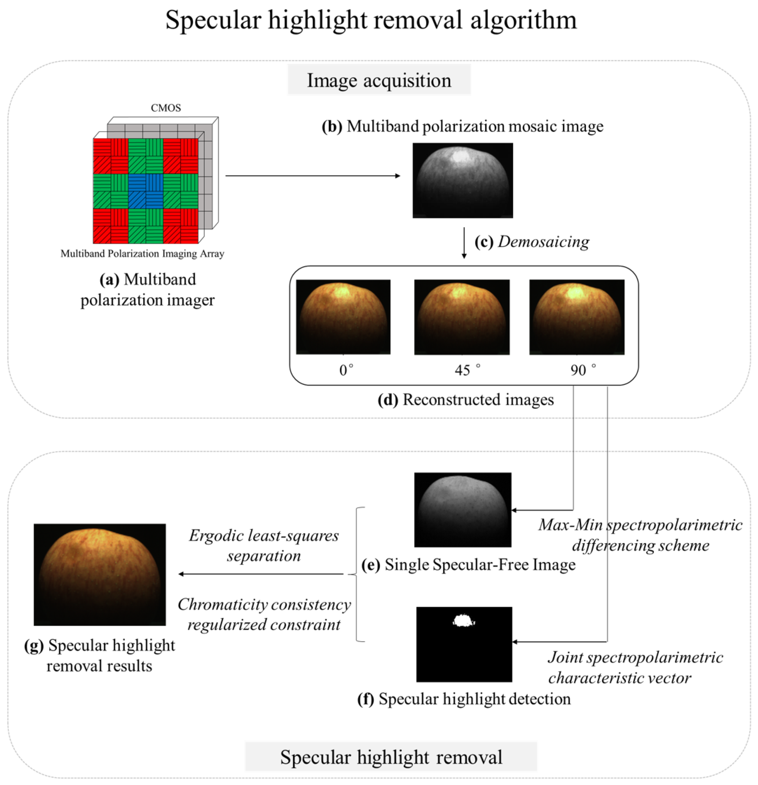
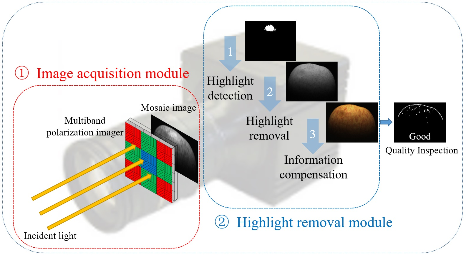
3. Methodology
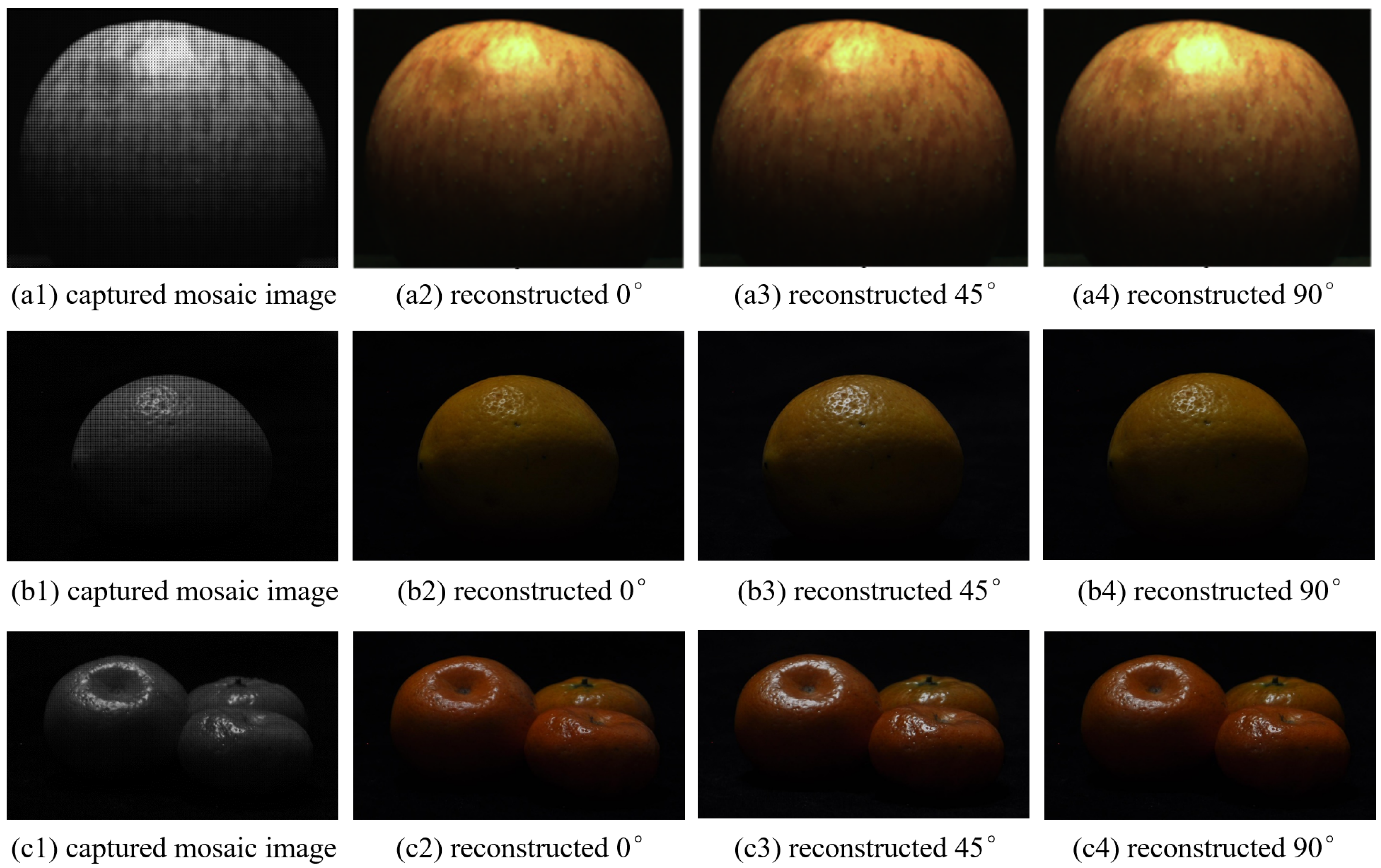
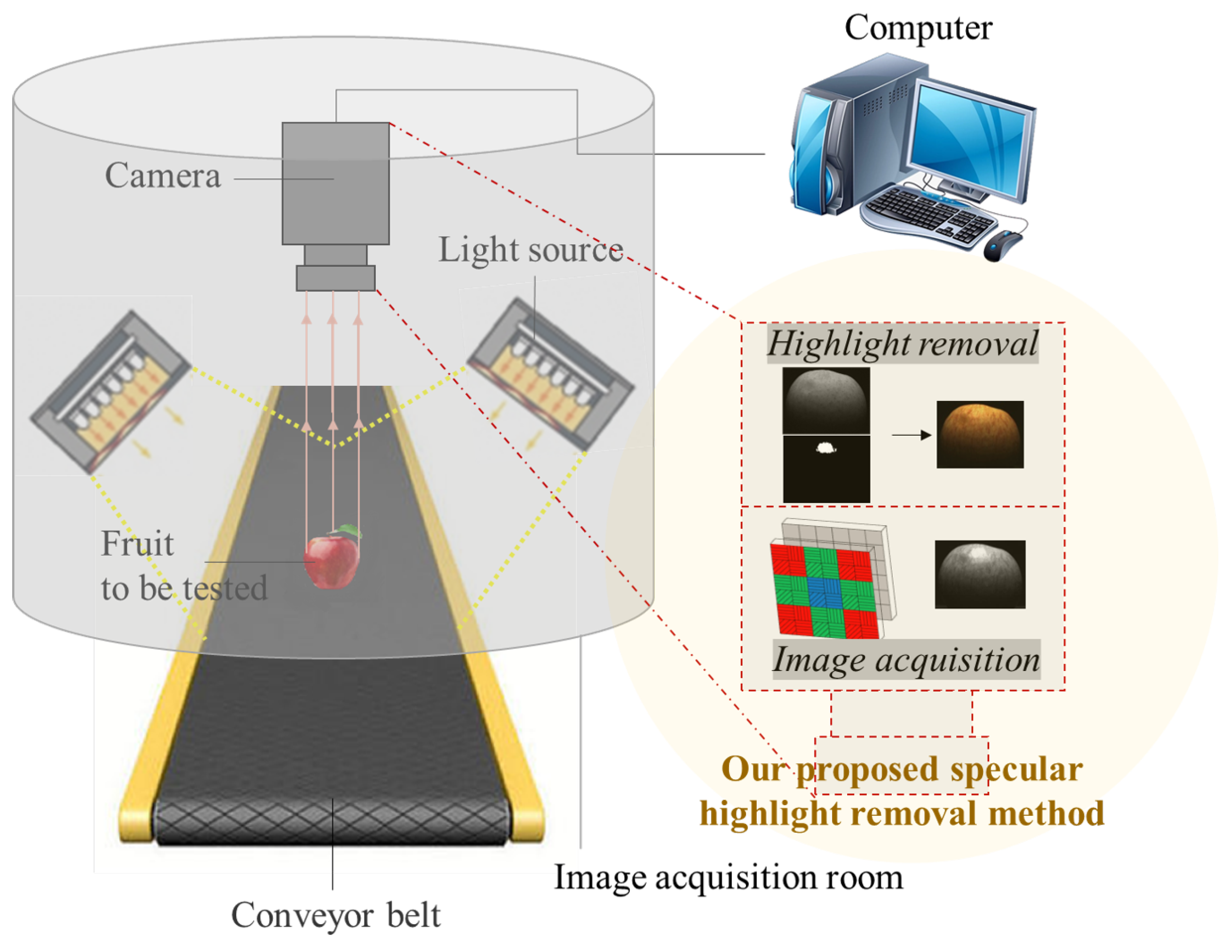
3.1. Images Acquisition Based on Multiband Polarization Imager
3.2. Specular Highlight Removal
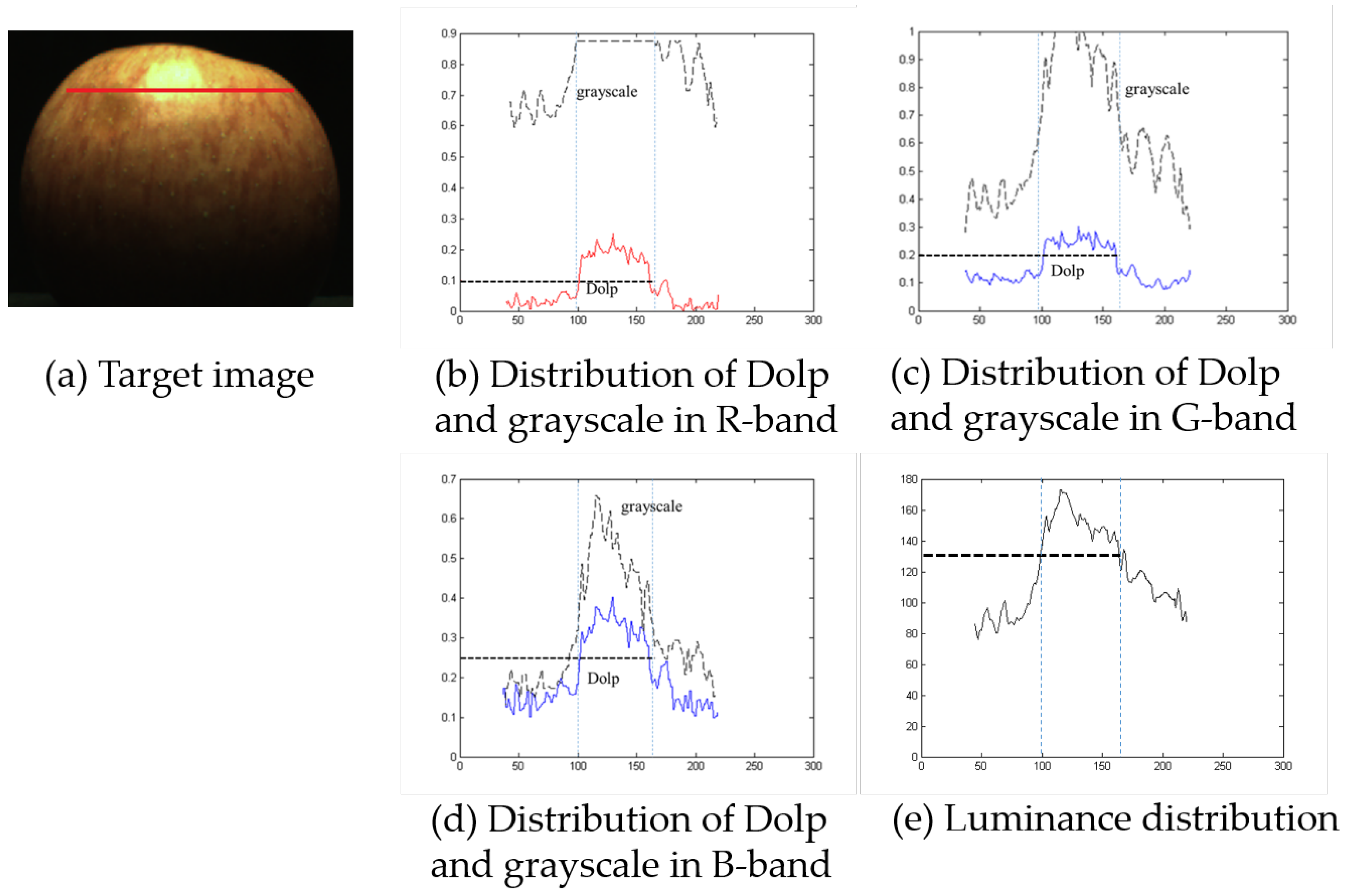
3.2.1. Highlight Detection Based on Multiband Polarization
3.2.2. Highlight Removal Based on Multiband Polarization
- a.
- Max-Min multi-band-polarization differencing scheme
- b.
- Ergodic least-squares separation algorithm
- c.
- The compensation of missing information based on local chromaticity consistency regularization constraint
- (1)
- Fixing and optimizing u
- (2)
- Fixing u and optimizing
4. Experiments and Results
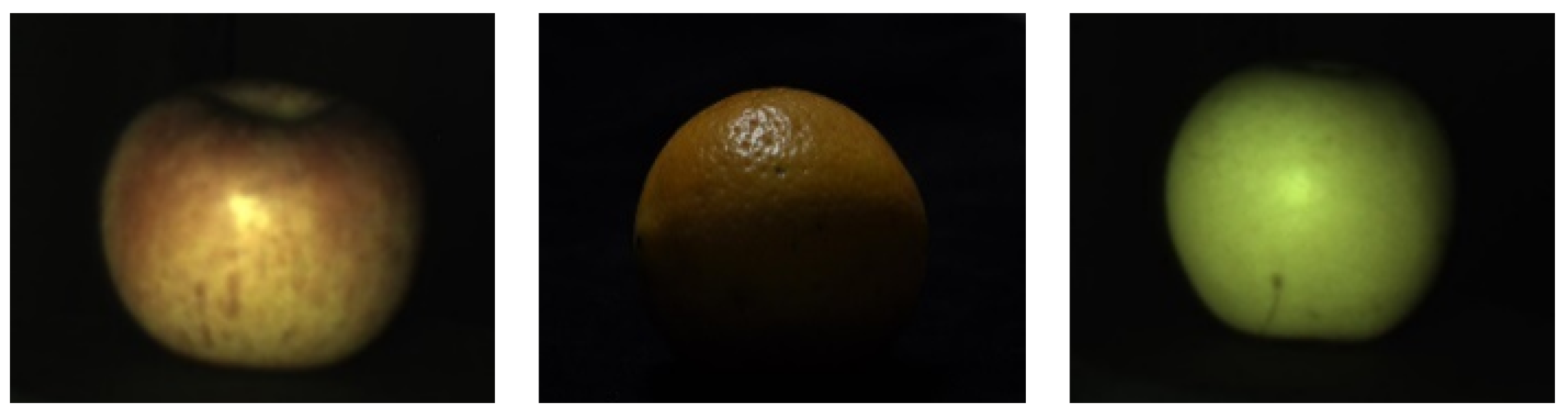
4.1. Experimental Data Acquisition
4.2. Objective Evaluation Results
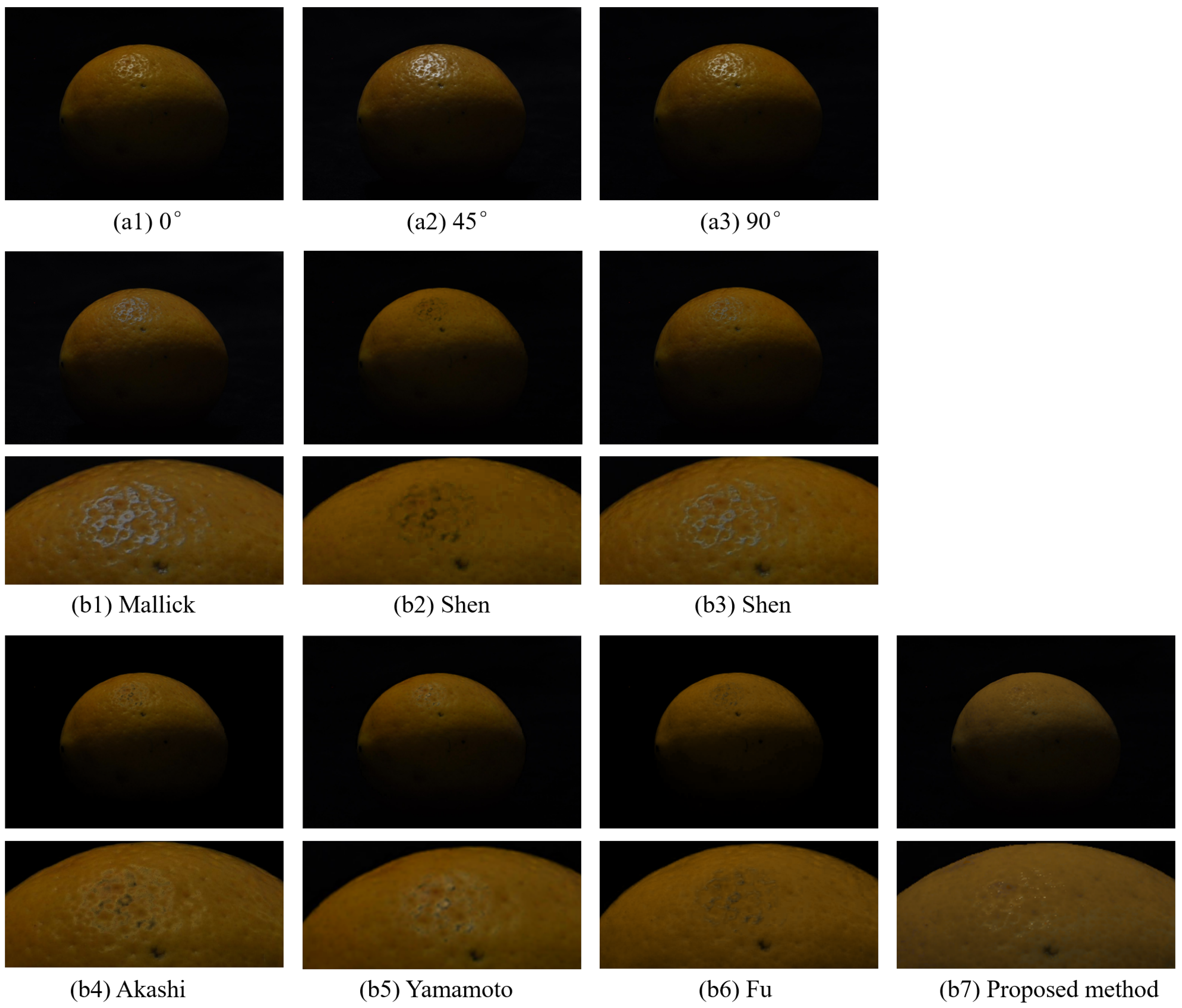
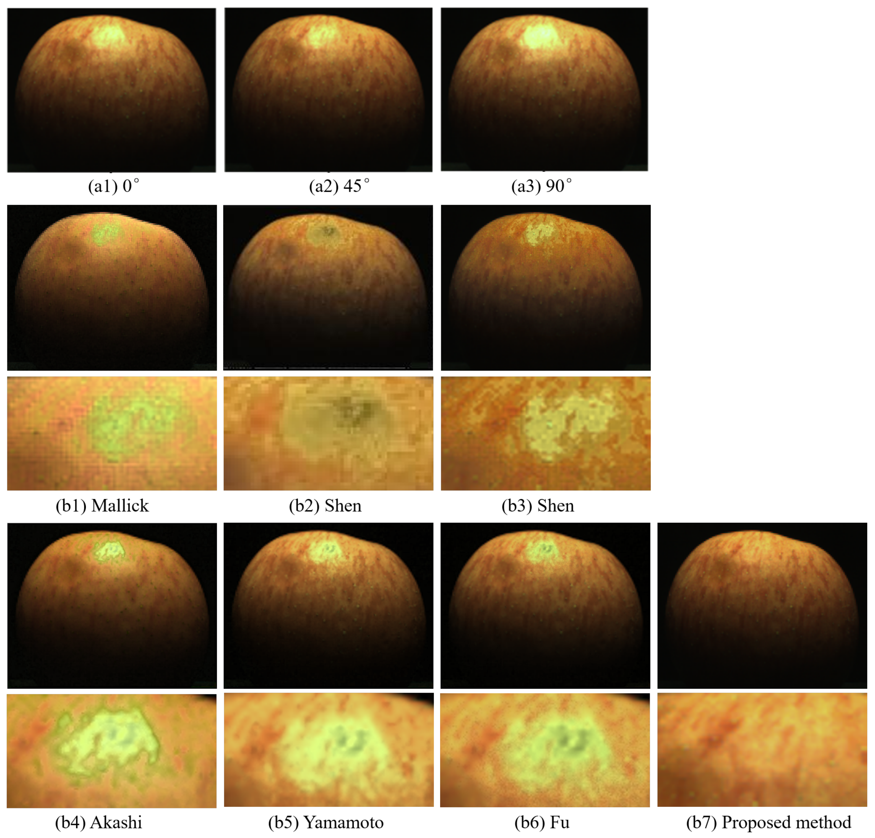
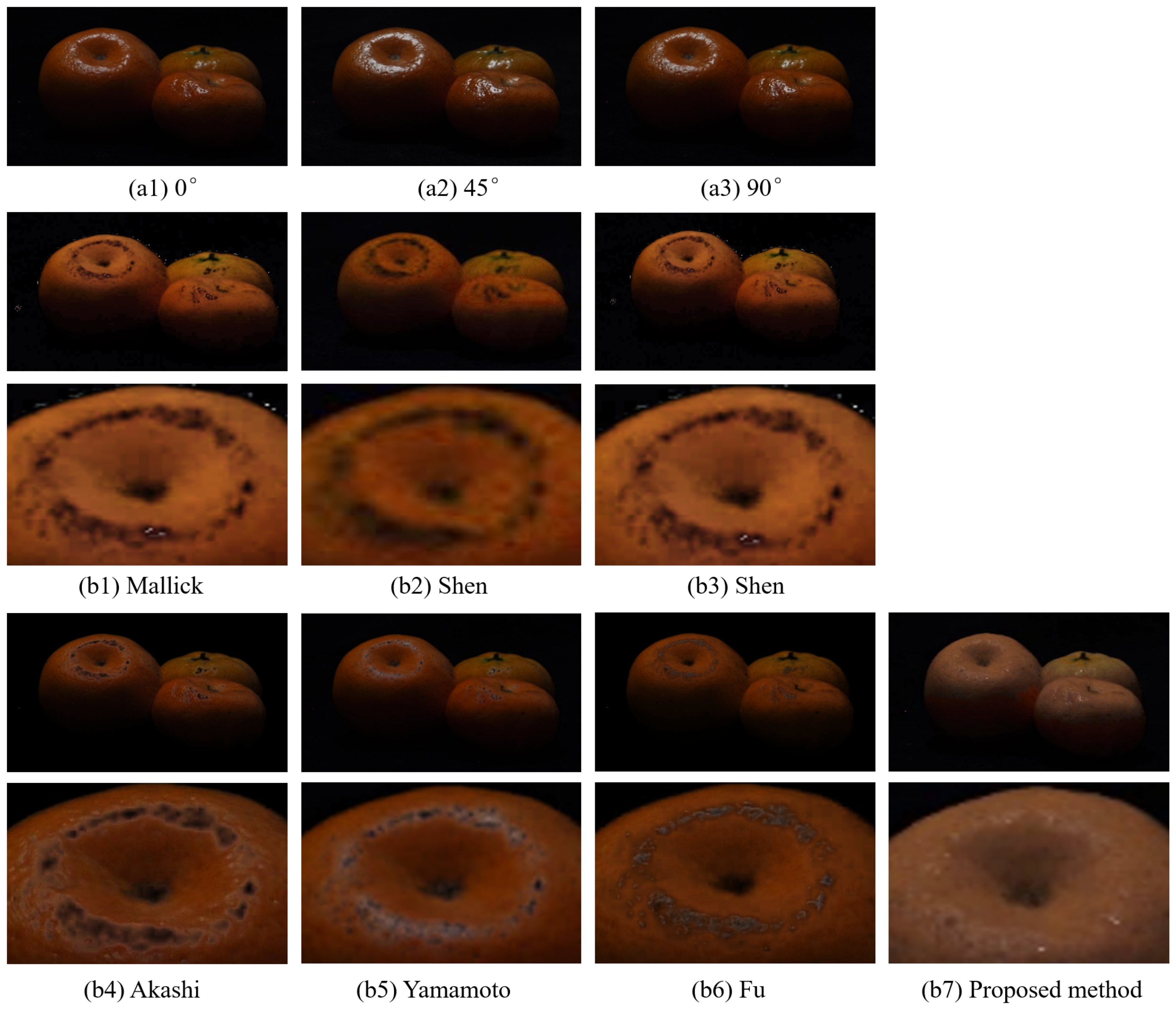
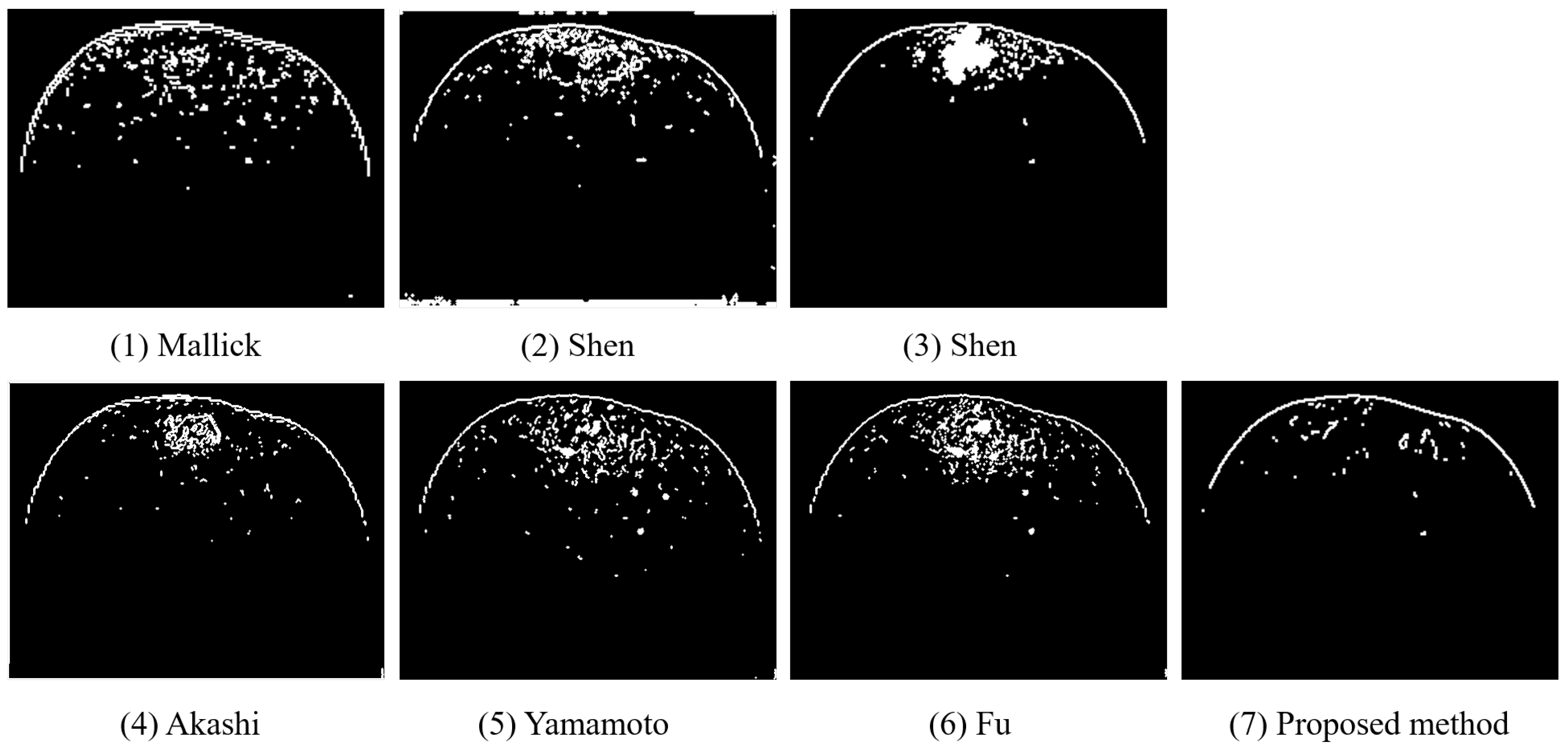
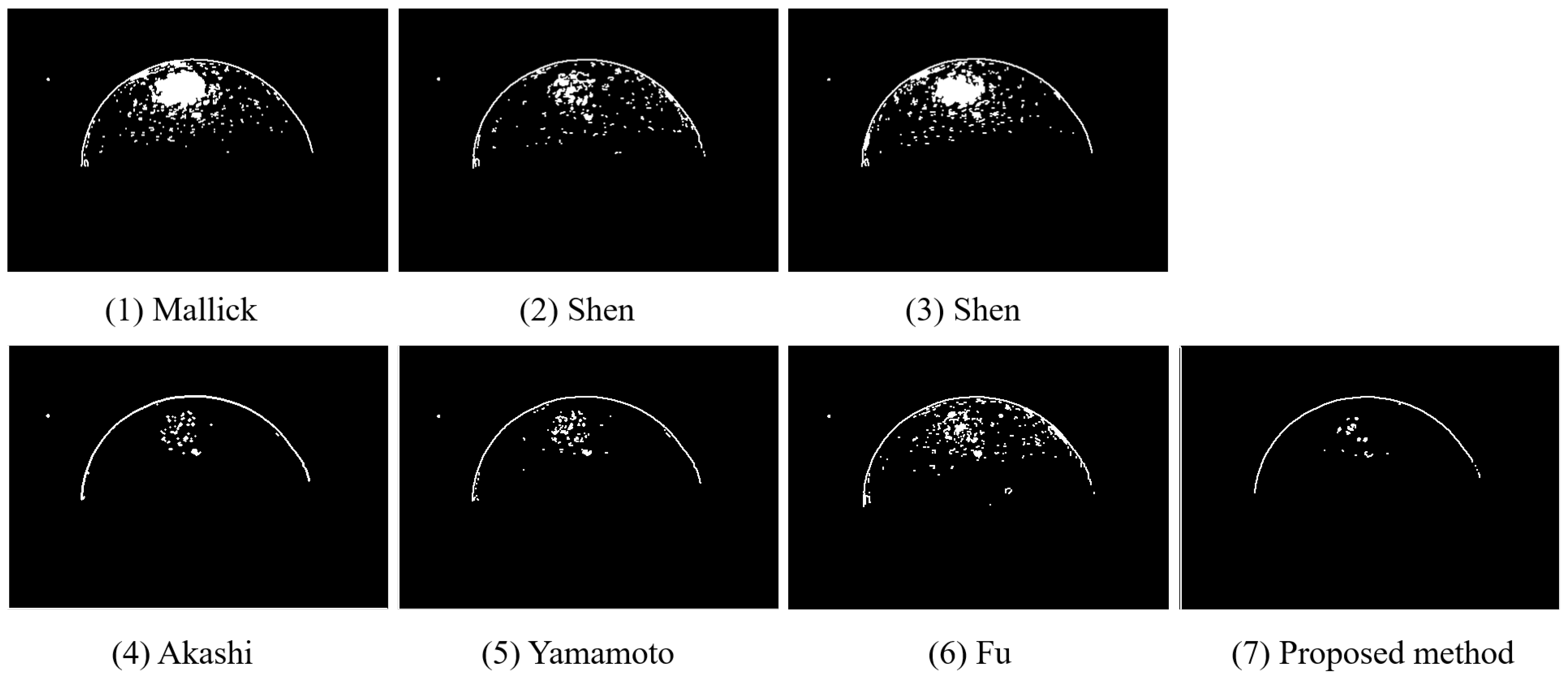
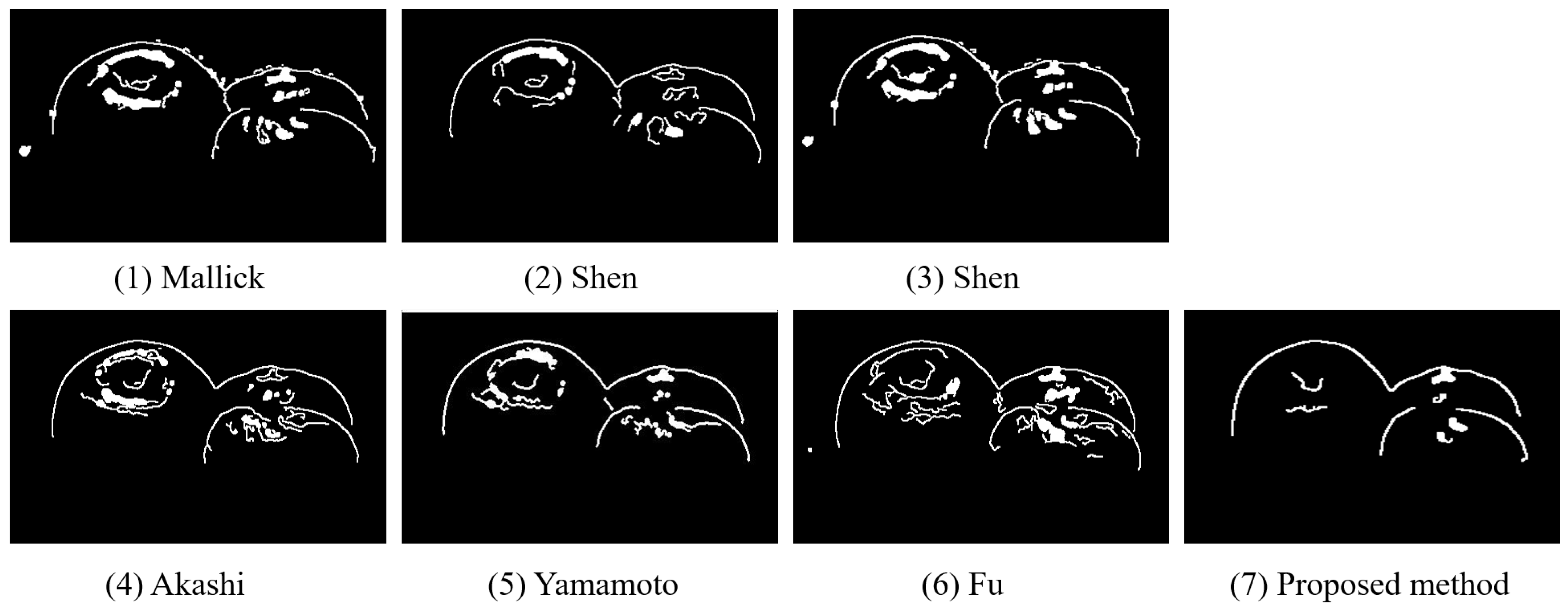
4.3. Specular Highlight Removal Results
4.4. Quality Inspection Results
5. Discussion
6. Conclusions
Author Contributions
Funding
Data Availability Statement
Acknowledgments
Conflicts of Interest
References
- Srivastava, S.; Sadistap, S. Non-destructive sensing methods for quality assessment of on-tree fruits: A review. J. Food Meas. Charact. 2018, 12, 497–526. [Google Scholar] [CrossRef]
- Qin, J.; Chao, K.; Kim, M.S.; Lu, R.; Burks, T.F. Hyperspectral and multispectral imaging for evaluating food safety and quality. J. Food Eng. 2013, 118, 157–171. [Google Scholar] [CrossRef]
- Sanaeifar, A.; Mohtasebi, S.S.; Ghasemi-Varnamkhasti, M.; Ahmadi, H. Application of MOS based electronic nose for the prediction of banana quality properties. Measurement 2016, 82, 105–114. [Google Scholar] [CrossRef]
- Maniwara, P.; Nakano, K.; Ohashi, S.; Boonyakiat, D.; Seehanam, P.; Theanjumpol, P.; Poonlarp, P. Evaluation of NIRS as non-destructive test to evaluate quality traits of purple passion fruit. Sci. Hortic. 2019, 257, 108712. [Google Scholar] [CrossRef]
- Vanakovarayan, S.; Prasanna, S.; Thulasidass, S.; Mathavan, V. Non-Destructive Classification of Fruits by Using Machine Learning Techniques. In Proceedings of the International Conference on System, Computation, Automation and Networking (ICSCAN), Pondicherry, India, 3–4 July 2021; pp. 1–5. [Google Scholar]
- Mohapatra, A.; Shanmugasundaram, S.; Malmathanraj, R. Grading of ripening stages of red banana using dielectric properties changes and image processing approach. Comput. Electron. Agric. 2017, 31, 100–110. [Google Scholar] [CrossRef]
- Li, Z.; Cui, G.; Chang, S.; Ning, X.; Wang, L. Application of computer vision technology in agriculture. J. Agric. Mech. Res. 2009, 31, 228–232. [Google Scholar]
- Artusi, A.; Banterle, F.; Chetverikov, D. A Survey of Specularity Removal Methods. Comput. Graph. Forum 2011, 30, 2208–2230. [Google Scholar] [CrossRef]
- Martinsen, P.; Schaare, P. Measuring soluble solids distribution in kiwifruit using near-infrared imaging spectroscopy. Postharvest Biol. Tec. 1998, 14, 271–281. [Google Scholar] [CrossRef]
- Nguyen-Do-Trong, N.; Keresztes, J.C.; De Ketelaere, B.; Saeys, W. Cross-polarised VNIR hyperspectral reflectance imaging system for agrifood products. Biosyst. Eng. 2016, 151, 152–157. [Google Scholar] [CrossRef]
- Wen, S.; Zheng, Y.; Lu, F.; Zhao, Q. Convolutional demosaicing network for joint chromatic and polarimetric imagery. Opt. Lett. 2019, 44, 5646–5649. [Google Scholar] [CrossRef]
- Shan, W.; Xu, C.; Feng, B. Image Highlight Removal based on Double Edge-preserving Filter. In Proceedings of the IEEE 5th International Conference on Signal and Image Processing (ICSIP), Nanjing, China, 3–5 July 2020. [Google Scholar]
- Shafer, S.A. Using color to separate reflection components. Color Res. Appl. 1985, 10, 210–218. [Google Scholar] [CrossRef] [Green Version]
- Attard, L.; Debono, C.J.; Valentino, G.; Castro, M.D. Specular Highlights Detection Using a U-Net Based Deep Learning Architecture. In Proceedings of the 2020 Fourth International Conference on Multimedia Computing, Networking and Applications (MCNA), Valencia, Spain, 19–22 October 2020; pp. 4–9. [Google Scholar]
- Bajcsy, R.; Lee, S.; Leonardis, A. Detection of diffuse and specular interface reflections and inter-reflections by color image segmentation. Int. J. Comput. Vis. 1996, 17, 241–272. [Google Scholar] [CrossRef] [Green Version]
- Tan, R.T.; Ikeuchi, K. Separating reflection components of textured surfaces using a single image. IEEE Trans. Pattern Anal. Mach. Intell. 2005, 27, 178–193. [Google Scholar] [CrossRef] [PubMed] [Green Version]
- Yang, Q.; Wang, S.; Ahuja, N. Real-time specular highlight removal using bilateral filtering. In Proceedings of the European Conference on Computer Vision, Crete, Greece, 5–11 September 2010. [Google Scholar]
- Mallick, S.P.; Zickler, T.; Belhumeur, P.; Kriegman, D. Dichromatic separation: Specularity removal and editing. In Proceedings of the ACM SIGGRAPH 2006 Sketches, Boston, MA, USA, 30 July–3 August 2006; p. 166. [Google Scholar]
- Shen, H.; Zhang, H.; Shao, S.; Xin, J. Chromaticity-based separation of reflection components in a single image. Pattern Recognit. 2008, 41, 2461–2469. [Google Scholar] [CrossRef]
- Yoon, K.J.; Choi, Y.; Kweon, I.S. Fast Separation of Reflection Components using a Specularity-Invariant Image Representation. In Proceedings of the IEEE International Conference on Image Processing, Atlanta, GA, USA, 8–11 October 2006; pp. 973–976. [Google Scholar]
- Shen, H.L.; Zheng, Z.H. Real-time highlight removal using intensity ratio. Appl. Opt. 2013, 52, 4483. [Google Scholar] [CrossRef] [Green Version]
- Kim, H.; Jin, H.; Hadap, S.; Kweon, I. Specular reflection separation using dark channel prior. In Proceedings of the IEEE Conference on Computer Vision and Pattern Recognition, Portland, OR, USA, 23–28 June 2013; pp. 1460–1467. [Google Scholar]
- Akashi, Y.; Okatani, T. Separation of reflection components by sparse non-negative matrix factorization. Comput. Vis. Image Underst. 2016, 146, 77–85. [Google Scholar] [CrossRef] [Green Version]
- Suo, J.; An, D.; Ji, X.; Wang, H.; Dai, Q. Fast and high quality highlight removal from a single image. IEEE Trans. Image Process. 2016, 25, 5441–5454. [Google Scholar] [CrossRef] [Green Version]
- Ren, W.; Tian, J.; Tang, Y. Specular reflection separation with color-lines constraint. IEEE Trans. Image Process. 2017, 26, 2327–2337. [Google Scholar] [CrossRef]
- Fu, G.; Zhang, Q.; Song, C.; Lin, Q.; Xiao, C. Specular highlight removal for real world images. Comput. Graph. Forum 2019, 38, 253–263. [Google Scholar] [CrossRef]
- Boyer, J.; Keresztes, J.C.; Saeys, W.; Koshel, J. An automated imaging BRDF polarimeter for fruit quality inspection. In Proceedings of the Novel Optical Systems Design and Optimization XIX, San Diego, CA, USA, 28 August 2016; pp. 82–90. [Google Scholar]
- Wen, S.; Zheng, Y.; Lu, F. Polarization Guided Specular Reflection Separation. IEEE Trans. Image Process. 2021, 30, 7280–7291. [Google Scholar] [CrossRef]
- Jian, S.; Yue, D.; Hao, S.; Yu, S.X. Learning non-lambertian object intrinsics across shapenet categories. In Proceedings of the IEEE Conference on Computer Vision and Pattern Recognition, Honolulu, HI, USA, 21–26 July 2017; pp. 1685–1694. [Google Scholar]
- Yi, R.; Tan, P.; Lin, S. Leveraging multiview image sets for unsupervised intrinsic image decomposition and highlight separation. In Proceedings of the Association for the Advance of Artificial Intelligence, New York, NY, USA, 7–12 February 2020; pp. 12685–12692. [Google Scholar]
- Nayar, S.K.; Fang, X.S.; Boult, T. Separation of reflection components using color and polarization. Int. J. Comput. Vis. 1997, 21, 163–186. [Google Scholar] [CrossRef]
- Nayar, S.K.; Fang, X.S.; Boult, T. Fast separation of direct and global components of a scene using high frequency illumination. ACM Trans. Graph. 2006, 25, 935–944. [Google Scholar] [CrossRef]
- Umeyama, S.; Godin, G. Separation of diffuse and specular components of surface reflection by use of polarization and statistical analysis of images. IEEE Trans. Pattern Anal. Mach. Intell. 2004, 26, 639–647. [Google Scholar] [CrossRef] [PubMed]
- Fan, W.; Ainouz, S.; Petitjean, C.; Bensrhair, A. Specularity removal: A global energy minimization approach based on polariza tion imaging. Comput. Vis. Image Underst. 2017, 158, 31–39. [Google Scholar]
- Yang, Y.; Wang, L.; Huang, M.; Zhu, Q.; Wang, R. Polarization imaging based bruise detection of nectarine by using ResNet-18 and ghost bottleneck. Postharvest Biol. Tec. 2022, 189, 111916. [Google Scholar] [CrossRef]
- Lin, S.; Li, Y.; Kang, S.; Tong, X.; Shum, H. Diffuse specular separation and depth recovery from image sequences. In Proceedings of the European Conference on Computer Vision, Copenhagen, Denmark, 28–31 May 2002. [Google Scholar]
- Lin, S.; Shum, H.Y. Separation of diffuse and specular reflection in color images. In Proceedings of the IEEE Conference on Computer Vision and Pattern Recognition, Kauai, HI, USA, 8–14 December 2001. [Google Scholar]
- Guo, X.; Cao, X.; Ma, Y. Robust separation of reflection from multiple images. In Proceedings of the IEEE Conference on Computer Vision and Pattern Recognition, Columbus, OH, USA, 23–28 June 2014; pp. 2187–2194. [Google Scholar]
- Nguyen-Do-Trong, N.; Dusabumuremyi, J.C.; Saeys, W. Cross-polarized VNIR hyperspectral reflectance imaging for non-destructive quality evaluation of dried banana slices, drying process monitoring and control. J. Food Eng. 2018, 238, 85–94. [Google Scholar] [CrossRef]
- Hao, J.; Zhao, Y.; Liu, W.; Kong, S.G.; Liu, G. A Micro-Polarizer Array Configuration Design Method for Division of Focal Plane Imaging Polarimeter. IEEE Sens. J. 2020, 21, 1. [Google Scholar] [CrossRef]
- Alenin, A.S.; Vaughn, I.J.; Tyo, J.S. Optimal bandwidth micropolarizer arrays. Opt. Lett. 2017, 42, 458. [Google Scholar] [CrossRef] [Green Version]
- Bai, C.; Li, J.; Lin, Z.; Yu, J. Automatic design of color filter arrays in the frequency domain. IEEE Trans. Image Process. 2016, 25, 1793–1807. [Google Scholar] [CrossRef]
- Zhao, X.; Lu, X.; Abubakar, A.; Bermak, A. Novel micro-polarizer array patterns for CMOS polarization image sensors. In Proceedings of the 2016 5th International Conference on Electronic Devices, Systems and Applications (ICEDSA), Ras Al Khaimah, United Arab, 6–8 December 2016; pp. 4994–5007. [Google Scholar]
- Bayer, B.E. Color Imaging Array. U.S. Patent 3,971,065, 20 July 1976. [Google Scholar]
- Shurcliff, W.A. Polarized Light: Production and Use; Harvard U. P.: Cambridge, MA, USA, 1962. [Google Scholar]
- Zhao, Y.; Peng, Q.; Xue, J.; Kong, S.G. Specular reflection removal using local structural similarity and chromaticity consistency. In Proceedings of the IEEE International Conference on Image Processing, Quebec City, QC, Canada, 27–30 September 2015. [Google Scholar]
- Afonso, M.V.; Bioucas-Dias, J.M.; Figueiredo, M.A. Fast Image Recovery Using Variable Splitting and Constrained Optimization. IEEE Trans. Image Process. 2010, 19, 2345–2356. [Google Scholar] [CrossRef] [Green Version]
- Buades, A.; Coll, B.; Morel, J.M. A non-local algorithm for image denoising. In Proceedings of the IEEE Computer Society Conference on Computer Vision and Pattern Recognition, San Diego, CA, USA, 20–26 June 2005. [Google Scholar]
- Yamamoto, T.; Kitajima, T.; Kawauchi, R. Efficient improvement method for separation of reflection components based on an energy function. In Proceedings of the IEEE International Conference on Image Processing, Beijing, China, 17–20 September 2017. [Google Scholar]
- Haralick, R.M. Textural Features for Image Classification. IEEE T. Syst. Man Cybern. 1973, 3, 610–621. [Google Scholar] [CrossRef] [Green Version]
- Ali, M.; Thai, K.W. Automated fruit grading system. In Proceedings of the IEEE International Symposium in Robotics and Manufacturing Automation, Kuala Lumpur, Malaysia, 19–21 September 2017; pp. 1–6. [Google Scholar]
- Ji, Y.; Zhao, Q.; Bi, S.; Shen, T. Apple Grading Method Based on Features of Color and Defect. In Proceedings of the 37th Chinese Control Conference (CCC), Wuhan, China, 25–27 July 2018; pp. 5364–5368. [Google Scholar]


| Mallick [18] | Shen [19] | Shen [21] | Akashi [23] | Yamamoto [49] | Fu [26] | Proposed | |
|---|---|---|---|---|---|---|---|
| AG | 0.2792 | 0.2622 | 0.2047 | 0.2282 | 0.2457 | 0.2523 | 0.3101 |
| ASM | 0.6290 | 0.6001 | 0.5986 | 0.6131 | 0.5869 | 0.6020 | 0.6335 |
| IDM | 0.9953 | 0.9969 | 0.9973 | 0.9958 | 0.9989 | 0.9965 | 0.9941 |
| Mallick [18] | Shen [19] | Shen [21] | Akashi [23] | Yamamoto [49] | Fu [26] | Proposed | |
|---|---|---|---|---|---|---|---|
| AG | 0.2468 | 0.2515 | 0.2499 | 0.2582 | 0.2601 | 0.2597 | 0.2826 |
| ASM | 0.7002 | 0.7065 | 0.7021 | 0.7030 | 0.7055 | 0.7064 | 0.7093 |
| IDM | 0.9971 | 0.9969 | 0.9963 | 0.9958 | 0.9957 | 0.9956 | 0.9948 |
| Mallick [18] | Shen [19] | Shen [21] | Akashi [23] | Yamamoto [49] | Fu [26] | Proposed | |
|---|---|---|---|---|---|---|---|
| AG | 0.2452 | 0.2285 | 0.2447 | 0.2382 | 0.2449 | 0.2503 | 0.2714 |
| ASM | 0.7164 | 0.7065 | 0.7119 | 0.7131 | 0.7187 | 0.7174 | 0.7182 |
| IDM | 0.9959 | 0.9979 | 0.9964 | 0.9969 | 0.9966 | 0.9957 | 0.9953 |
| Mallick [18] | Shen [19] | Shen [21] | Akashi [23] | Yamamoto [49] | Fu [26] | Proposed | |
|---|---|---|---|---|---|---|---|
| AG | 0.2605/0.0249 | 0.2487/0.0222 | 0.2235/0.0209 | 0.2381/0.0245 | 0.2488/0.0267 | 0.2583/0.0278 | 0.2921/0.0194 |
| ASM | 0.6196/0.0373 | 0.6725/0.0368 | 0.6085/0.0357 | 6780/0.0341 | 0.6120/0.0387 | 0.6753/0.0402 | 0.6855/0.0358 |
| IDM | 0.9951/0.0010 | 0.9973/0.0012 | 0.9964/0.0009 | 0.9967/0.0010 | 0.9950/0.0012 | 0.9956/0.0014 | 0.9945/0.0009 |
| Mallick [18] | Shen [19] | Shen [21] | Akashi [23] | Yamamoto [49] | Fu [26] | Proposed | |
|---|---|---|---|---|---|---|---|
| Results | Damage | Damage | Damage | Damage | Damage | Damage | Good |
| Mallick [18] | Shen [19] | Shen [21] | Akashi [23] | Yamamoto [49] | Fu [26] | Proposed | |
|---|---|---|---|---|---|---|---|
| Results | Damage | Damage | Damage | Good | Good | Damage | Good |
Publisher’s Note: MDPI stays neutral with regard to jurisdictional claims in published maps and institutional affiliations. |
© 2022 by the authors. Licensee MDPI, Basel, Switzerland. This article is an open access article distributed under the terms and conditions of the Creative Commons Attribution (CC BY) license (https://creativecommons.org/licenses/by/4.0/).
Share and Cite
Hao, J.; Zhao, Y.; Peng, Q. A Specular Highlight Removal Algorithm for Quality Inspection of Fresh Fruits. Remote Sens. 2022, 14, 3215. https://doi.org/10.3390/rs14133215
Hao J, Zhao Y, Peng Q. A Specular Highlight Removal Algorithm for Quality Inspection of Fresh Fruits. Remote Sensing. 2022; 14(13):3215. https://doi.org/10.3390/rs14133215
Chicago/Turabian StyleHao, Jinglei, Yongqiang Zhao, and Qunnie Peng. 2022. "A Specular Highlight Removal Algorithm for Quality Inspection of Fresh Fruits" Remote Sensing 14, no. 13: 3215. https://doi.org/10.3390/rs14133215
APA StyleHao, J., Zhao, Y., & Peng, Q. (2022). A Specular Highlight Removal Algorithm for Quality Inspection of Fresh Fruits. Remote Sensing, 14(13), 3215. https://doi.org/10.3390/rs14133215