Soil Moisture Retrieval Using SAR Backscattering Ratio Method during the Crop Growing Season

Abstract

Soil moisture content (SMC) is an indispensable basic element for crop growth and development in agricultural production. Obtaining accurate information on SMC in real time over large agricultural areas has important guiding significance for crop yield estimation and production management. In this study, the paper reports on the retrieval of SMC from RADARSAT-2 polarimetric SAR data. The proposed SMC retrieval algorithm includes vegetation correction based on a ratio method and roughness correction based on the optimal roughness method. Three vegetation description parameters (i.e., RVI, LAI, and NDVI) serve as vegetation descriptors in the parameterization of the algorithm. To testify the vegetation correction result of the algorithm, the water cloud model (WCM) was compared with the algorithm. The calibrated integrated equation model (CIEM) was employed to describe the backscattering from the underlying soil. To improve the accuracy of SMC retrieval, the CIEM model was optimized by using the optimal roughness parameter and the normalization method of reference incidence angle. Validation against ground measurements showed a high correlation between the measured and estimated SMC when the NDVI serves as vegetation descriptor (R² = 0.68, RMSE = 4.15 vol.%, p < 0.01). The overall estimation performance of the proposed SMC retrieval algorithm is better than that of the WCM. It demonstrates that the proposed algorithm has an operational potential to estimate SMC over wheat fields during the growing season.

1. Introduction

Soil moisture content (SMC) is an important parameter in the change process of land surface systems, playing a critical role in agricultural management, surface water cycling, and energy exchange in near-earth space [1,2,3,4,5]. SMC is an indispensable basic element for crop growth and development in agricultural production. The SMC can be used as an effective index of farmland health. The content of soil moisture is directly related to the health status of crops. Drought can lead to soil drying and cracking, hinder crop growth, reduce crop yield, and threaten food security. Therefore, access to accurate SMC information on farmland is of great significance for crop yield estimation, drought monitoring, and agricultural production management. Traditionally, SMC monitoring and investigation methods were ground-based point measurements or interpolated lines or grids. The implementation is not only time-consuming and labor-intensive, but also difficult to obtain spatially continuous soil moisture information in time, which has great limitations for its operational use [6]. Satellite remote sensing has the advantages of being fast, macro, and dynamic, providing an effective means to obtain soil moisture information.

For visible-infrared bands, the SMC estimation is from the relationships between soil spectral reflectance and soil moisture or vegetation traits occur under water stress, such as the single spectral analysis method [7,8,9] and the vegetation index method [10,11,12]. For thermal-infrared bands, the SMC is derived from the parameters related to the soil thermal properties, such as the thermal inertia method [13,14,15] and the temperature index method [16,17]. However, the optical/thermal methods are associated with some inherent limitations, such as vegetation interference, night effects, poor temporal resolution, and cloudy conditions [18]. Comparing with optical/thermal remote sensing, Synthetic Aperture Radar (SAR) has all-weather day-and-night penetration capabilities, and can provide effective and cost-efficient means of monitoring and assessing SMC over vegetation cover conditions [19,20,21]. SAR remote sensing retrieves SMC by establishing relationships between the radar backscattering coefficient and soil moisture, because the amount of water held in the soil is directly proportional to the dielectric constant of soil [22]. The basis of SMC retrieval is the soil dielectric constant. However, besides the soil dielectric constant, SAR signal is also affected by other factors, such as surface roughness, vegetation cover, and radar system parameters. Therefore, if we only pay attention to the relationship between soil moisture and the SAR backscattering coefficient and ignore the influence of other parameters, we can only obtain a trend of overall change, which is far from meeting the requirements of SMC retrieval. There are still some challenges in retrieving SMC using SAR data over vegetated areas. The observed SAR signals include the combined information of vegetation moisture and SMC because the vegetation canopy contains water [23,24]. The vegetation canopy volume scattering, the interaction between soil and vegetation and the observed backscattering are highly nonlinear [25,26,27], which increases the difficulty of SMC retrieval. When using SAR to retrieve SMC under vegetation cover, the SMC is underestimated if vegetation effect is not considered [28,29]. Therefore, removing the influence of vegetation is the key in SMC retrieval using SAR.

To remove the vegetation effects, a number of methods has been established by scholars. These methods can be generally classified into two categories: methods based on polarization decomposition and methods based on vegetation scattering models [30]. Hajnsek et al. [31] used surface, dihedral, and vegetation scattering to interpret the scattering processes and to retrieve SMC. The potential of using polarimetric decompose for estimating volumetric SMC under agricultural vegetation was proved. Combining polarimetric decomposition techniques with the concept of multi-angularity, Jagdhuber et al. proposed a retrieval technique for SMC under low vegetation cover [32]. He et al. estimated SMC in agricultural crop fields from fully polarimetric SAR data through the polarimetric decomposition of a SAR coherency matrix. Martino et al. [33] used a polarimetric two-scale two-component model (PTSTCM) to describe the surface scattering component, and a randomly (uniformly, vertically, or horizontally) oriented thin-dipole model to describe the volume scattering contribution from the vegetation layer that covers the scattering surface. The problem of negative power in SMC retrieval is significantly mitigated. It is noteworthy that polarization decomposition method for soil moisture retrieval requires fully polarization data. Vegetation scattering models describing the scattering processes of microwave signals have been established (such as Michigan microwave canopy scattering (MIMICS) [34]; Water cloud model (WCM) [35]; the distorted Born approximation (DBA) [36]; the Tor Vergata model (TVM) [37]), which can also be used to remove the influence of vegetation cover on soil moisture retrieval. Among these models, WCM has been widely used for SMC retrieval over vegetated areas because it only requires a few parameters and has high accuracy [30].

SAR backscattering includes mixed signals of vegetation and soil from agricultural fields, while vegetation contributions vary at different growth stages [38]. In addition, soil surface roughness also affects radar backscattering [39]. Over vegetated areas, soil surface roughness cannot be easily measured directly, which has caused some problems for soil moisture retrieval. Therefore, the key issue in the quantitative estimation of SMC is to separate the effect of vegetation and soil roughness. In this paper, a method was developed to retrieve SMC over agriculture fields during the crop growing season. The proposed method combined the optimal roughness method and ratio method. The ratio method was used to separate the scattering contribution of vegetation from total backscattering. The vegetation correction procedure is embedded within a SMC retrieval algorithm, in which the surface scattering component is formulated by the Calibrated Integrated Equation Model (CIEM) [40]. For the problem that roughness cannot be measured, the optimal roughness was defined by a global search method. Finally, the developed method is applied to estimate SMC over agriculture fields. In addition, the proposed model was compared with the WCM to evaluate its effectiveness and accuracy.

2. Materials

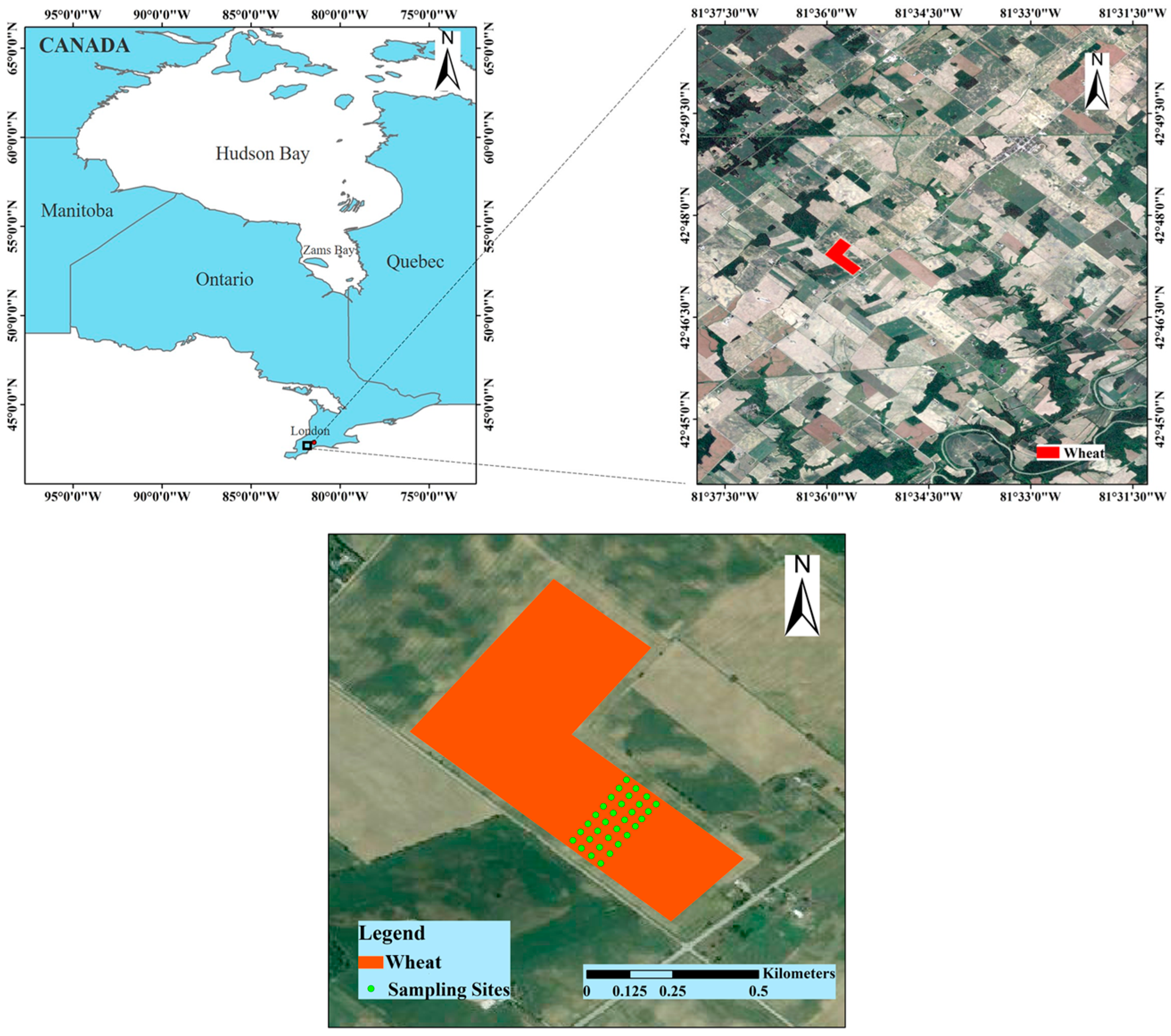
2.1. Ground Measurements

The study area is a relatively flat agricultural region located at London (Longitude: 81°5′W, Latitude: 42°7′N), southwestern Ontario, Canada (Figure 1). The selected area is a rain-fed agricultural area; therefore, SMC will not be affected by irrigation.

Field campaigns were conducted in the study area from May to July in 2019 simultaneously with each RADARSAT-2 SAR data acquisition. A total of eight field visits was carried out, and 240 sample data were collected throughout the wheat growing season. Selected photos taken during in the field campaigns are shown in Figure 2. The spatial distance between any two adjacent sampling points is no less than 30 m. A time domain reflectometry (TDR) instrument was used to measure the SMC (vol.%) at 0–5 cm of the soil surface. Each sampling point was measured six times, and the average value of the six measurements was taken as the soil moisture reading of the sampling location. Real-time kinematic (RTK) carrier phase division technology was used to record the longitude and latitude information of each sampling point, so that the image parameter information corresponding to the sampling point can be extracted from the remote sensing image. The leaf area index (LAI) was extracted by using an optical fisheye camera (Nikon d300s) with a focal length of 10.5 mm and can-eye software. Unfortunately, due to instrument failure, the LAI could not be obtained on June 16. In addition, the normal difference vegetation index (NDVI) was extracted from Sentinel-2. However, in the two days before and after the SAR observation, only six cloudless optical images were available (

Table 1. Acquisition date of SAR and optical images.

SAR Acquisition Date	Optical Image Acquisition Date
9 May 2019	/
16 May 2019	15 May 2019
20 May 2019	/
29 May 2019	27 May 2019
2 June 2019	4 June 2019
9 June 2019	11 June 2019
16 June 2019	14 June 2019
10 July 2019	9 July 2019

).

2.2. RADARSAT-2 Data

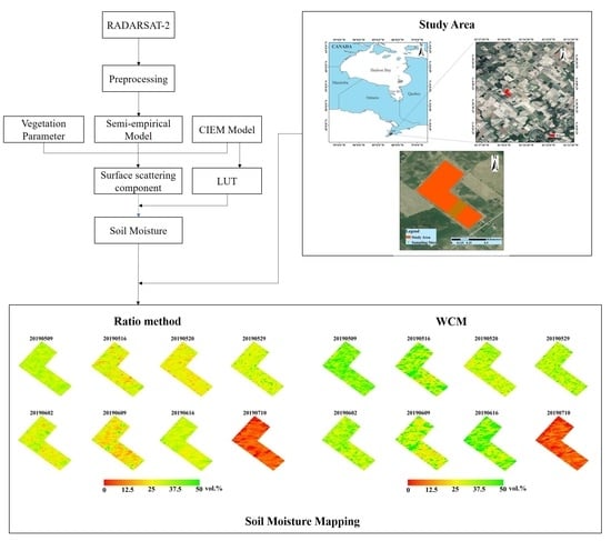
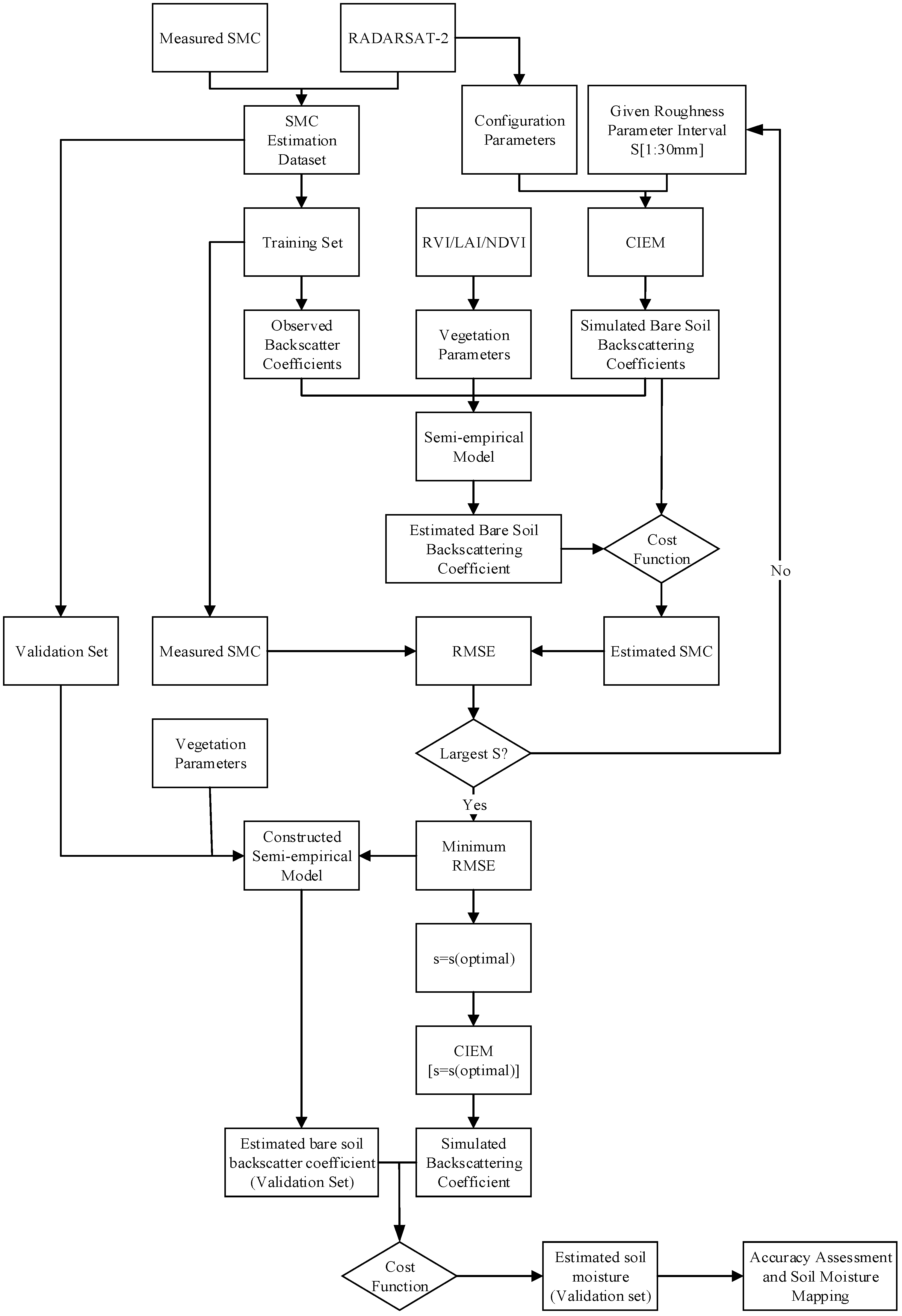
During the wheat growing season (May–July 2019), eight RADARSAT-2 SAR images acquired over the study area were provided by the Canadian Space Agency through the SOAR (Science and Operational Applications Research) program. The nominal spatial resolution of RADARSAT-2 images was approximately 8 m. The satellite revisit period was 24 days, and the orbit period was 100.7 min. For details of the acquired RADARSAT-2 SAR images, please see reference [20]. The RADARSAT-2 SAR preprocessing mainly includes radiometric calibration and speckle filtering.

The local incidence angle of SAR usually has an effect on the surface backscattering coefficient, which should not be ignored in SMC estimation. In order to limit the influence of different local incident angles, the theoretical method proposed by Ulaby et al. [41], which is based on Lambert’s law for optics [42], was used to normalize the backscattering coefficients in this study:

$${\mathsf{\sigma }}_{{\theta }_{ref}}^{°}={\mathsf{\sigma }}_{\theta }^{°}\times \frac{co{s}^2{\theta }_{ref}}{co{s}^2\theta } ,$$

(1)

where $\theta$is the local incidence angle, and ${\theta }_{ref}$ is the reference incidence angle.

3. Methods

In this study, the scattering model CIEM was used to simulate the backscattering coefficients of soil surface covered by winter wheat. After the vegetation correction, the soil moisture estimation and accuracy verification were carried out using a look-up table approach. The workflow of SMC retrieval is shown in Figure 3. The specific experiment included the following steps:

(1) The model was constructed based on the observed total coefficients, the vegetation parameters (e.g., RVI, LAI and NDVI), and the bare soil backscattering coefficients simulated by the CIEM model. Then, the undetermined coefficients of the model were fitted using the least-squares method.

(2) For each sampling date, 70% of the data were randomly selected as the training set and the rest as the validation set. Basic statistics (e.g., mean, standard deviation, etc.) of the training and validation sets were calculated and compared, and they were not statically different.

(3) After fitting the undetermined coefficients of the model, the estimated bare soil backscattering could be obtained. Using a look-up table approach, the SMC of the training set was estimated based on the minimum cost function strategy (Equation (2)) and the simulated bare soil backscatter coefficients. Then the RMSE between the measured and estimated SMC was calculated as the estimation accuracy of SMC on the training set.

$$\cos \mathrm{t}=\min \left\{\sqrt{{\left({\sigma }_{HHsoil}^{°}-{\sigma }_{HHCIEM}^{°}\right)}^2+{\left({\sigma }_{VVsoil}^{°}-{\sigma }_{VVCIEM}^{°}\right)}^2} \right\} ,$$

(2)

(4) All the RMS heights (s) within the given roughness parameter interval were traversed and steps (1) and (2) repeated until s reached the maximum value in the given range. The estimation accuracy of SMC on the training set was then compared with different s, and the s with the highest estimation accuracy was taken as the optimal roughness parameter of the study area on the sampling date. The optimal roughness was taken as the effective roughness of the model.

(5) For the validation set, the estimated backscattering coefficients of bare soil were obtained using the constructed model. Then the SMC of the validation set was estimated using the minimum cost function strategy and the backscattering coefficients of bare soil simulated by the CIEM model with the optimal roughness parameter. Finally, the accuracy evaluation was conducted using the measured SMC on the validation set.

(6) The SMC mapping of the study area was conducted using the constructed model.

3.1. Vegetation Correction

3.1.1. Ratio Method

The ratio of bare soil backscattering contribution to the observed backscattering can be affected by vegetation cover and remote sensing sensor configuration [43]. Therefore, for areas with vegetation cover, when the sensor configuration parameters were fixed, the ratio of the surface backscattering to the total backscattering coefficients was only related to some vegetation description parameters, which can be expressed using the following equation:

$$\frac{{\sigma }_{ppsoil}^{°}}{{\sigma }_{pp}^{°}}=F\left(\mathrm{vegetation} \mathrm{paramter}\right) ,$$

(3)

where pp represents the HH or VV polarization mode, ${\sigma }_{ppsoil}^{°}$ is the backscattering coefficient of bare soil, and ${\sigma }_{pp}^{°}$ represents the total backscattering coefficient.

The ratio function F on the right side of Equation (3) does not have a fixed expression form. Scholars have used a variety of ratio functions in order to better characterize the backscattering contribution of vegetation in the ratio equation [3,43,44]. A combination of the power exponential function and linear function could better characterize the vegetation scattering [45].

$$F=aV+b{V}^c ,$$

(4)

where V is the vegetation description parameter, a, b and c are the undetermined coefficients of the ratio function.

For the selection of vegetation description parameters in the ratio function, the current research has not reached a consistent conclusion. Some studies believed that the vegetation water content (VWC) had a strong attenuation effect on the scattered radiation of the microwave signal in the vegetation layer, so VWC was suitable for vegetation parameter description. There is a strong correlation between radar vegetation index (RVI) and VWC [46]. The RVI can be obtained directly from SAR images without being affected by weather conditions. Therefore, RVI was selected as the vegetation parameter to parameterize the ratio function in this study. The definition of RVI is shown as follows:

$$\mathrm{RVI}=\frac{8{\sigma }_{HV}^{°}}{{\sigma }_{HH}^{°}+{\sigma }_{VV}^{°}+{\sigma }_{HV}^{°}} ,$$

(5)

where${\sigma }_{HV}^{°}$, ${\sigma }_{HH}^{°}$ and ${\sigma }_{VV}^{°}$ are the backscattering coefficient of different polarization modes. In addition to RVI, leaves have been considered to be able to control the scattering and attenuation of microwave signals in the canopy to a certain extent [39], especially for herbaceous vegetation. Therefore, LAI was used to describe the scattering characteristics of vegetation. NDVI can well represent vegetation greenness information, reflecting a growth state of vegetation, and does not depend on field measurements which can be obtained from optical remote sensing data. Therefore, NDVI was also used to parameterize the ratio function. These three vegetation parameters were compared with for the SMC estimation performance. LAI was derived from field measurements, and NDVI was extracted from Sentinel-2. Since the data of LAI and NDVI did not cover all sampling dates, only the SMC of the sampling dates with data was estimated when using these two parameters.

3.1.2. WCM

The WCM is a semi-empirical backscattering model proposed by Attema and Ulaby [35]. The WCM divides the observed total backscattering into the three parts: the vegetation canopy scattering component, the multiple scattering component between vegetation and the soil surface, and the surface scattering component attenuated by the vegetation, which can be expressed as follows:

$$\begin{array}{c} {\sigma }_{can}^{°}={\sigma }_{veg}^{°}+{\sigma }_{veg+soil}^{°}+{\tau }^2{\sigma }_{soil}^{°} ,\\ {\sigma }_{veg}^{°}=A{V}_{1}cos\theta \left(1-{\tau }^2\right) ,\\ {\tau }^2=exp\left(\frac{-2B{V}_2}{cos\theta }\right) ,\end{array}$$

(6)

where${\sigma }_{can}^{°}$ is the observed total backscattering coefficient, ${\sigma }_{veg}^{°}$ is the scattering component from the vegetation canopy, ${\sigma }_{veg+soil}^{°}$ is the multiple scattering component formed between vegetation and soil, and ${\sigma }_{soil}^{°}$ is the surface scattering component attenuated by vegetation layer. ${\tau }^2$ represents the two-way attenuation through the vegetation canopy. A and B are the undetermined coefficients of the model, which are generally obtained by least-squared fitting according to the measured data. $V_1$ and $V_2$ represent the direct scattering and the attenuation properties of vegetation, respectively. In this study, $V_1$ and $V_2$ were parameterized by the three vegetation parameters (RVI, LAI and NDVI) that were used to construct the ratio function. Among the scattering components in the WCM model, ${\sigma }_{veg+soil}^{°}$ accounts for a very small proportion compared to the remaining two components, which can usually be ignored.

Using the McLaughlin series to expand the parameter${\tau }^2$, the WCM can be further simplified [47].

$${\tau }^2=\exp \left(\frac{-2BV}{cos\theta }\right)=1-\frac{2BV}{cos\theta }+\frac{2B^2{V}^2}{co{s}^2\theta }+\dots ,$$

(7)

Ignoring the multiple scattering components between soil and vegetation, and retaining the first two terms of the McLaughlin series expansion, the WCM can be expressed as follows:

$${\sigma }_{can}^{°}=2AB{V}^2+\left(1-\frac{2BV}{cos\theta }\right){\sigma }_{soil}^{°},$$

(8)

Taking ${\sigma }_{can}^{°}$ as the dependent variable and ${\sigma }_{soil}^{°}$ as the independent variable, let a = 2AB and b = −2B/cos$\theta$, Equation (8) can be simplified to the following expression:

$${\sigma }_{soil}^{°}=\frac{ {\sigma }_{can}^{°}-a{V}^2}{bV+1} ,$$

(9)

where V represents the vegetation description parameter. According to the simplified WCM model (Equation (9)), the functional relationship between the backscattering coefficient of bare soil and the total backscattering coefficient can be established after obtaining the undetermined coefficients.

3.2. Surface Backscatter Modeling

3.2.1. CIEM Model

The integrated equation model (IEM) is a highly applicable bare soil scattering model [48], which constructs the functional relationship between co-polarized backscattering coefficients and surface roughness parameters (e.g., RMS height (s) and correlation length (L)), incident angle and wavelength, and soil dielectric constant. The field measurement of the surface RMS height (s) and correlation length (L) are greatly affected by human factors. Baghdadi et al. [40] constructed the functional expression between s and L based on a large number of roughness data from field surveys and C-band SAR data combined with simulated value of IEM model, and proposed a calibrated integrated equation model (CIEM), which reduced the dependence on s or L.

The empirical relationship between correlation length and RMS height in the CIEM model establish for C-band SAR can be expressed as follows:

$$L\left(s, \theta , pp\right)=a{\left(sin\theta \right)}^b{s}^{\left(c\theta +d\right)} ,$$

(10)

where L is the surface correlation length, s is RMS height, pp is the HH or VV polarization mode, and a, b, c and d are the undetermined coefficients. According to the different polarization modes, the values are as follows:

$$\begin{array}{c}{a}_{HH}=4.026, d_{HH}=1.551, a_{VV}=3.289, d_{VV}=1.222,\\ b_{HH}=b_{VV}=-1.774, c_{HH}=b{c}_{VV}=-0.0025,\end{array}$$

(11)

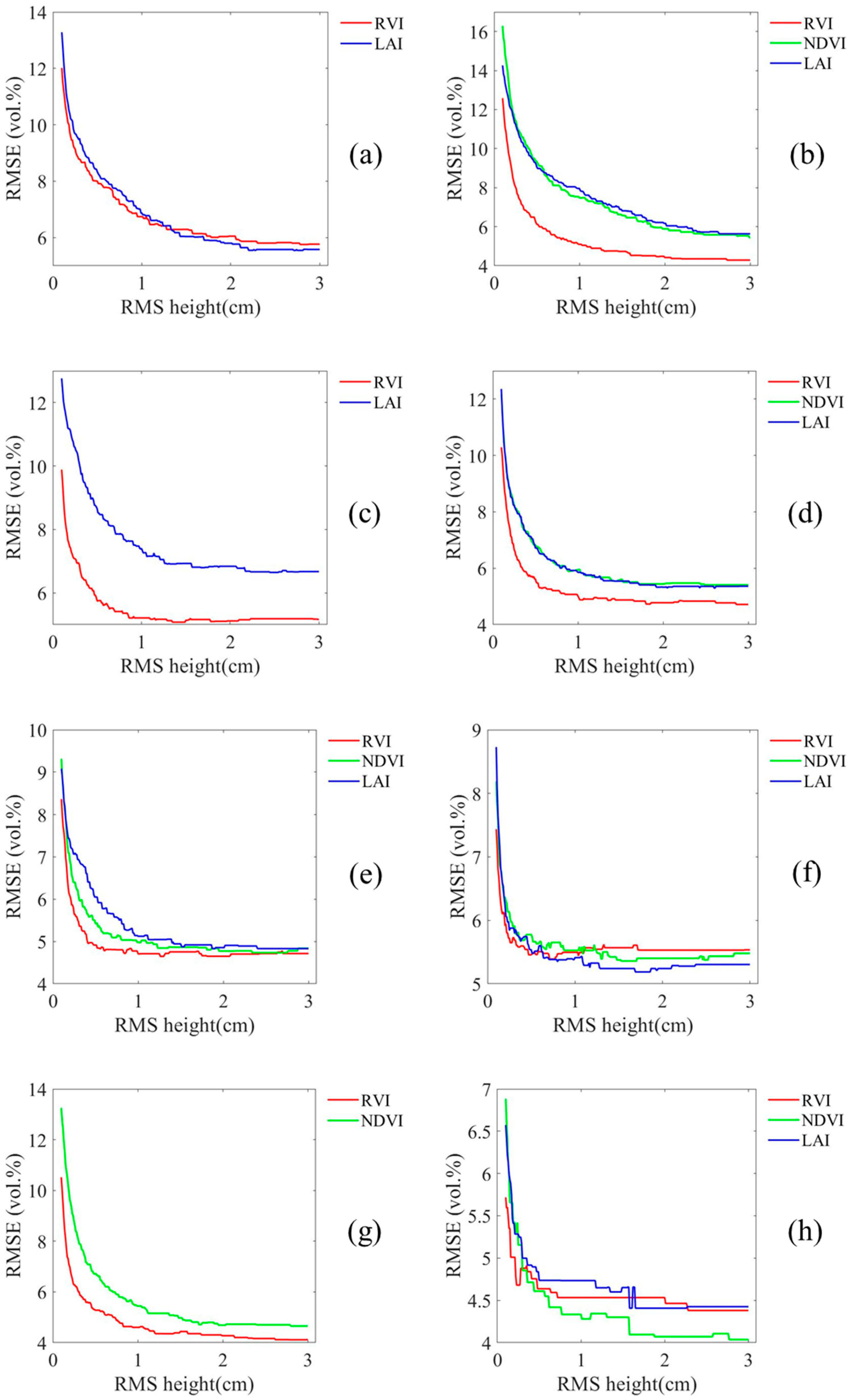
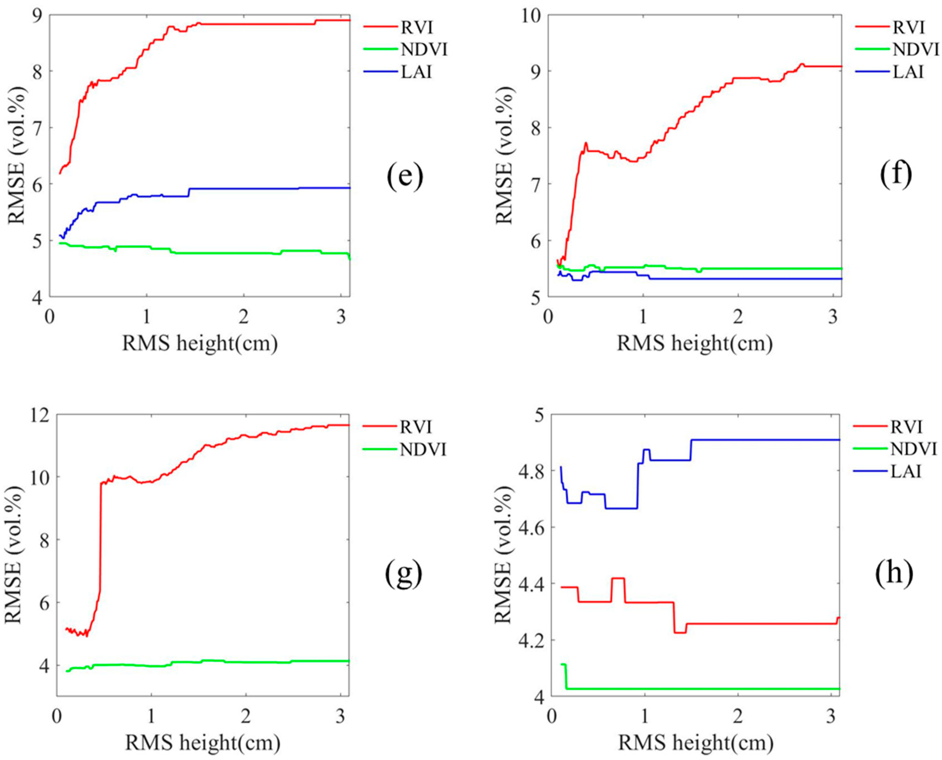
3.2.2. Optimal Roughness Parameters

The correlation length (L) in the CIEM is expressed as an empirical function of the RMS height (s), reducing the number of unknown roughness parameters. Therefore, only the s was used as the roughness parameter in this study. The roughness parameter is an important parameter in microwave scattering model of bare soil. However, the measurement process of roughness parameters is complex and easily affected by human factors and the measuring instruments used, especially in densely vegetated areas [49]. In this study, the optimal roughness parameter based on the global search method [50] was used to parameterize the bare soil scattering model. The idea of this method is to assume that the roughness parameters in the study area have constant values during a certain period of time. The solution process of the optimal roughness parameters adopts the following method: given a roughness parameter range, for this study, the range of the RMS height was set to 1 mm–30 mm and the step size was 1 mm. Then the bare soil scattering model was constructed using the roughness parameter within the given range to estimate SMC. The SMC estimation accuracy with different roughness conditions was obtained, and finally the RMS height corresponding to the highest estimation accuracy was taken as the optimal roughness parameter of the study area. For the estimation of the overall SMC in the study area, the optimal roughness parameter was essentially used as an empirical parameter of the bare soil scattering model to improve the estimation performance of the overall SMC, and there would be deviations from the real roughness parameters at different locations in the study area. Therefore, it could not represent the real roughness conditions of all sampling points.

3.3. Accuracy Assessment

The accuracies of different models were compared and evaluated using statistical indicators, including the coefficient of determination (R², Equation (12)) and the root-mean-square error (RMSE, Equation (13)).

$${\mathrm{R}}^2=1-\frac{{\displaystyle \sum _{i=1}^n{(y_i-{\widehat{y}}_i)}^2}}{{\displaystyle \sum _{i=1}^n{(y_i-\overline{y})}^2}}$$

(12)

$$\mathrm{RMSE}=\sqrt{{\displaystyle \sum _{i=1}^n\frac{{(y_i-{\widehat{y}}_i)}^2}{n}}}$$

(13)

where n is the number of sample points; $y_i$ and ${\widehat{y}}_i$ represent the measured SMC value and estimated SMC value of the i-th sample site respectively; and $\overline{y}$ is the mean value of the measured SMC values.

4. Results and Discussion

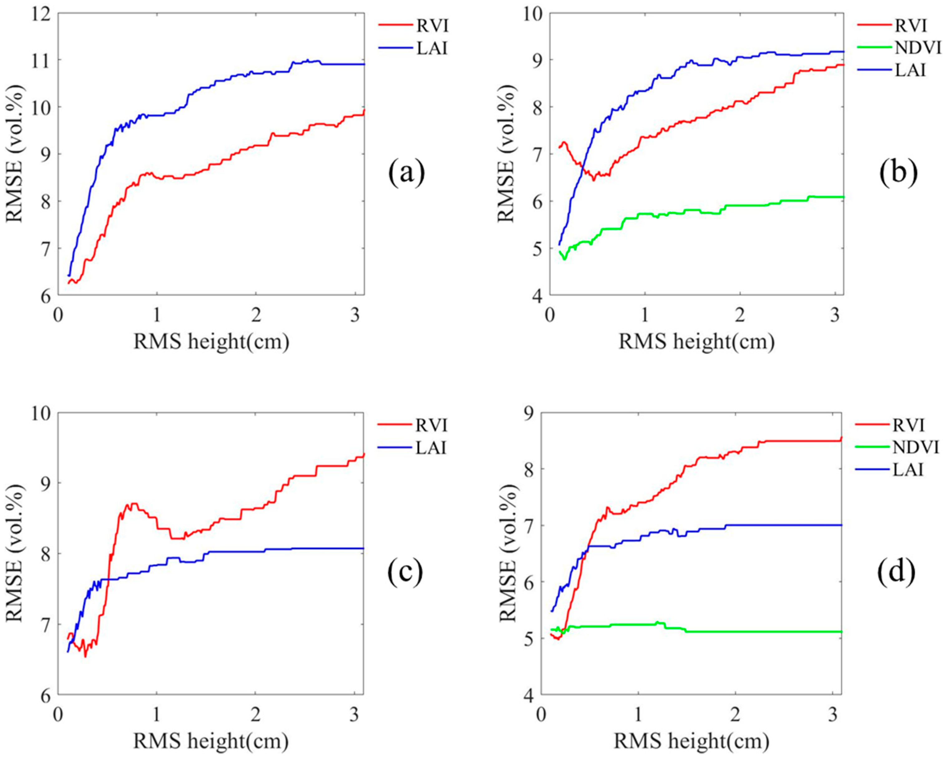
4.1. Optimal Roughness Parameter Selection

The SMC estimation accuracies on the training set with different RMS heights and different vegetation parameters were obtained (Figure 4 and Figure 5). Figure 4 and Figure 5 show the RMSE of the estimation results on the training set of different sampling dates when the model was the ratio method and WCM, respectively. When the RMSE reached the minimum, the RMS height corresponding to the horizontal axis was considered to be the optimal roughness parameter in the current phase.

Table 2. Fitting coefficients of semi-empirical models based on RVI, LAI and NDVI.

Vegetation Parameters	Semi-Empirical Models	Sampling Date	HH			VV
			a	b	c	a	b	c
RVI	Ratio method/WCM	9 May	0.28/−0.85	0.21/179.04	−1.09/	−0.40/−0.44	0.85/24.95	0.25/
		16 May	0.62/−1.18	0.06/8.94	−1.72/	0.53/−0.15	0.13/−0.08	−1.02/
		20 May	0.36/−0.76	0.30/13.50	−1.11/	0.28/−0.09	0.24/0.49	−0.85/
		29 May	−11.92/−0.51	12.25/18.26	0.92/	−6.85/−0.25	7.17/3.43	0.87/
		2 June	0.38/−0.38	0.26/97.41	−0.72/	0.36/−0.27	0.12/15.82	−1.18/
		9 June	0.32/−0.53	0.52/52.86	−0.58/	−0.2/−0.09	0.78/4.07	0.16/
		16 June	0.13/−0.39	0.33/5.95	−0.45/	0.09/0.03	0.36/−0.70	−0.2/
		10 July	0.46/−0.22	0.28/1.16	−1.30/	0.08/−2.16	0.72/15.24	−0.32/
LAI	Ratio method/WCM	9 May	0.83/−0.77	0.05/81.16	−1.39/	0.78/−0.44	0.04/14.48	−1.63/
		16 May	0.44/−0.28	0.13/108.07	−1.70/	−16.46/−0.16	17.02/16.78	0.97/
		20 May	−3.92/−0.16	4.48/83.29	0.91/	−4.77/−0.06	5.26/8.82	0.93/
		29 May	−0.05/−0.07	0.57/22.56	0.15/	−0.53/−0.04	0.96/4.29	0.67/
		2 June	0.20/−0.10	0.39/14.93	−1.83/	0.21/−0.08	0.40/3.90	−3.60/
		9 June	−2.97/−0.11	3.58/5.74	0.87/	−3.05/−0.05	3.56/1.05	0.89/
		10 July	0.45/−0.03	70.21/1.57	−12.55/	0.42/−1.23	4.24/31.73	−6.23/
NDVI	Ratio method/WCM	16 May	0.35/−1.95	0.15/77.68	−1.26/	0.99/−0.86	0.00/14.68	−10.33/
		29 May	−14.13/−1.10	14.53/25.03	0.93/	−2.66/−3.84	3.19/40.17	0.92/
		2 June	−1.53/−0.52	1.75/0.27	0.10/	−0.42/−0.54	0.70/0.47	−0.35/
		9 June	−17.08/−0.46	17.67/1.15	0.94/	−14.20/−0.21	14.67/−0.02	0.94/
		16 June	−1.26/−7.09	1.79/1532	0.85/	−4.85/−0.19	5.29/14.94	0.90/
		10 July	−8.45/−1197	8.13/124,336	0.67/	−15.51/−5718	14.79/184,373	0.75/

shows the fitting coefficients of the two models (Ratio method and WCM) with the condition of optimal roughness parameters.

Table 3. The value of optimal roughness parameter when different vegetation parameters were used as vegetation description parameters (Ratio method).

Date	Optimal Roughness Parameter (cm)
	RVI	NDVI	LAI
9 May	2.78.	/	2.71
16 May	2.73	2.99	2.64
20 May	1.35	/	2.45
29 May	2.86	2.49	2.05
2 June	1.26	2.34	1.87
9 June	0.71	1.53	1.69
16 June	2.78	2.80	/
10 July	2.28	2.77	1.58

and

Table 4. The value of optimal roughness parameter when different vegetation parameters were used as vegetation description parameters (WCM).

Date	Optimal Roughness Parameter (cm)
	RVI	NDVI	LAI
9 May	0.10	/	0.12
16 May	0.46	0.15	0.10
20 May	0.28	/	0.10
29 May	0.18	0.22	0.12
2 June	0.10	3.00	0.14
9 June	0.13	1.57	0.26
16 June	0.32	0.10	/
10 July	1.32	0.16	0.58

show the optimal roughness parameters of the study area for different sampling dates when using the ratio method and WCM.

As shown in Figure 4 and Figure 5, the SMC estimation accuracy was jointly affected by the vegetation parameters and the RMS height. For the ratio method, no matter which vegetation parameters was used as the input parameter of the model, the RMSE curve on the training set is generally parabolic, and it shows a trend of rapid decline at first and then a much gentler trend (See Figure 4). It shows that the estimation accuracy of SMC was more sensitive to the change of the RMS height when the RMS height was small.

As shown in Table 3, when different vegetation parameters were used to parameterize the ratio method, different values of the optimal roughness parameter were obtained. It is noteworthy that the values of optimal roughness parameters obtained on most sampling dates were large. Figure 4 shows that RMSE decreases with an increase in optimal roughness parameters. The variation of backscattering coefficients simulated by the CIEM with the RMS heights is not linear, the RMSE on the training set estimated by the ratio method was not strictly monotonically decreasing. The RMSE of estimated SMC would reach the global minimum with a smaller roughness parameter on some dates.

As shown in Figure 5, For WCM, the RMSE variation curves estimated on the training set are significantly different from that obtained from the ratio method. When RVI or LAI was used the vegetation parameter, the estimated RSME curves shows an upward trend on most sampling dates. With the gradual increase of the RMS height, the change of the RMSE tended to be gentle, the sensitivity of estimation accuracy to the change in RMS height decreased, and the estimation accuracy reached the highest when the roughness was low. When NDVI was used as vegetation description parameter, the RMSE curves of the training set on different dates almost tended to be horizontal; that is, the estimation accuracy did not change significantly with the increase in RMS height. As shown in Figure 5h, for the SMC estimation of the training set on July 10, the estimation performance with three vegetation parameters has little change with different RMS heights. This is because the value of measured SMC on July 10 was low, and the backscattering of the bare soil simulated by CIEM is not sensitive to the change of the RMS height, so that the estimated SMC values with different roughness conditions were almost the same. As shown in Table 4, comparing with the ratio method, the optimal roughness of WCM was smaller. It suggested that the optimal roughness parameter not only changed with the vegetation parameters and the acquisition time of the SAR data, but also depended on the models used in the estimation process to describe the scattering characteristics of vegetation. In general, the optimal roughness parameter, as an empirical coefficient in the scattering model, can effectively improve the estimation performance of the SMC.

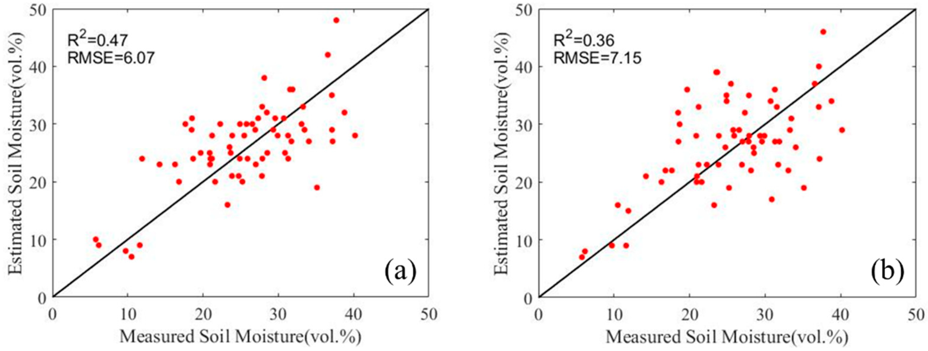
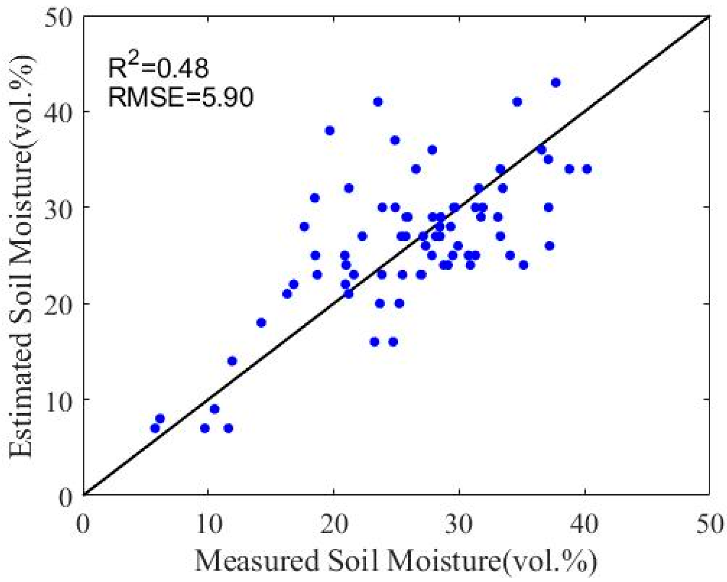
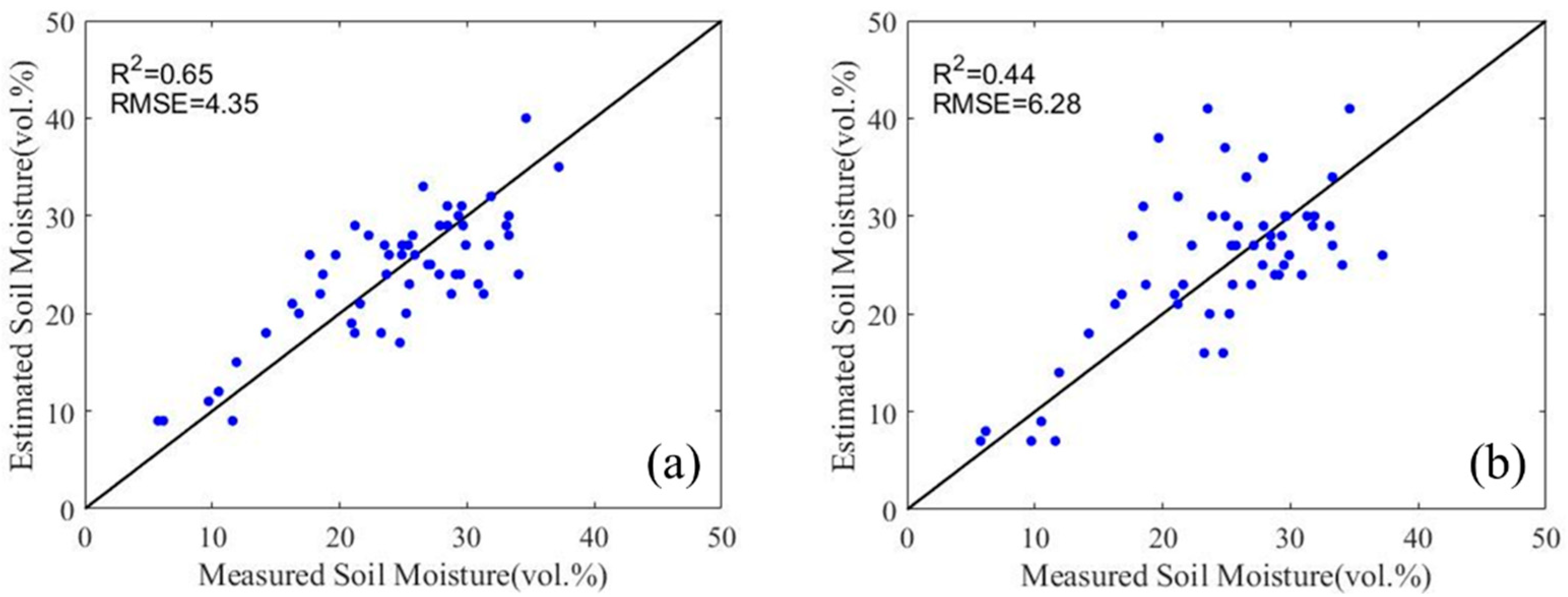
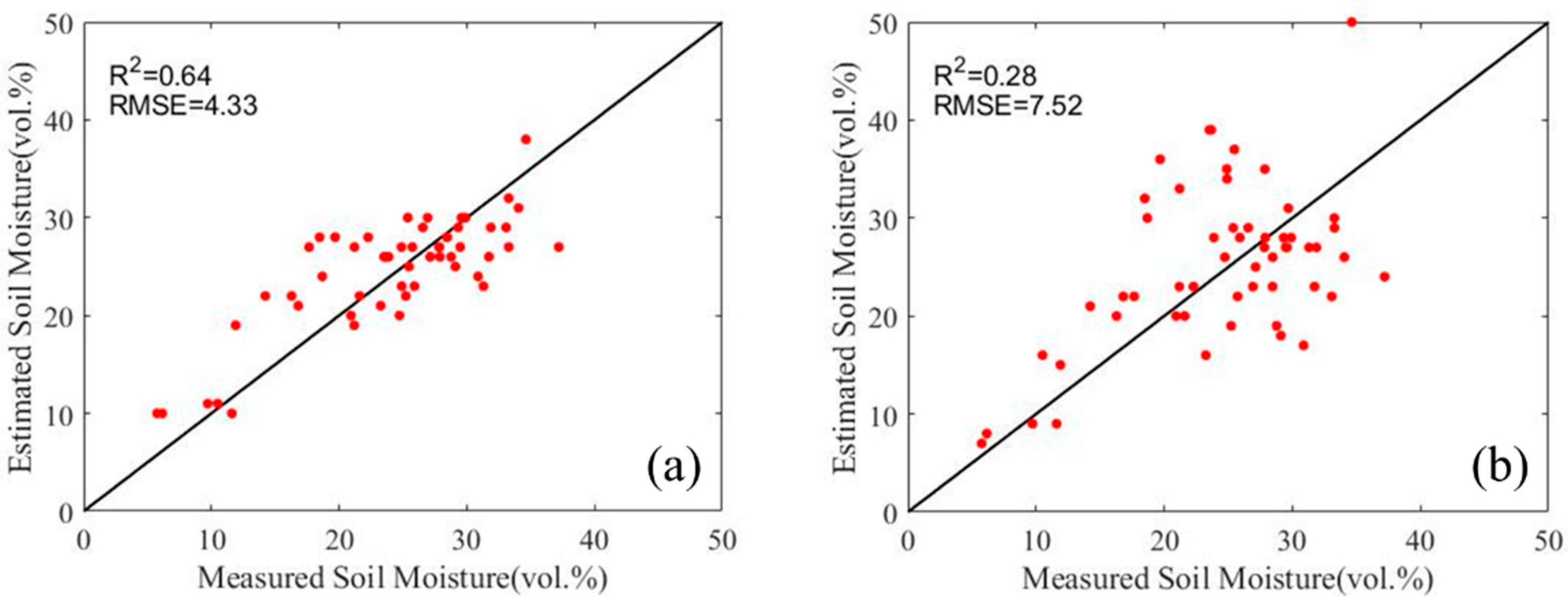
4.2. Soil Moisture Estimation Results

Figure 6, Figure 7, Figure 8, Figure 9, Figure 10 and Figure 11 show the scatter plots between the measured and the estimated SMC on the validation set from ratio method or WCM using different vegetation parameters.

Table 5. Estimation accuracy of validation set (comparison between LAI, NDVI, and RVI).

Vegetation Correction Model	Vegetation Parameters	R2	RMSE (vol.%)
Ratio method	RVI (all dates)	0.48	5.90
	LAI/RVI (exclude 16 June)	0.56/0.48	5.58/6.15
	NDVI/RVI (exclude 9 May, 20 May)	0.65/0.44	4.35/6.28
	LAI/NDVI (exclude 9 May, 20 May, 16 June)	0.57/0.65	5.27/4.43
WCM	RVI (all dates)	0.34	7.17
	LAI/RVI (exclude 16 June)	0.47/0.36	6.07/7.15
	NDVI/RVI (exclude 9 May, 20 May)	0.64/0.28	4.33/7.52
	LAI/NDVI (exclude 9 May, 20 May, 16 June)	0.52/0.62	5.45/4.63

shows the estimation accuracy of SMC on the validation set. Since the data of LAI and NDVI did not cover all sampling dates, when comparing the estimation accuracy under different vegetation parameters, only the sampling dates that contained vegetation parameters data were compared.

As shown in Figure 6, Figure 7, Figure 8, Figure 9, Figure 10 and Figure 11 and Table 5, the accuracy of SMC retrieval was the lowest when RVI was used as vegetation descriptor (for ratio method, R² = 0.48, RMSE = 5.90 vol.%; for WCM R² = 0.34, RMSE = 7.17 vol.%). The accuracy of SMC retrieval was the highest when NDVI was used as vegetation descriptor (for ratio method, R² = 0.65, RMSE = 4.35 vol.%; for WCM R² = 0.64, RMSE = 4.33 vol.%). In order to compare the estimation performances of models parameterized by RVI, LAI and NDVI, the SMC estimation accuracies were studied. Since NDVI data were not available for 9 May and 20 May and LAI data were not available for 6 June, these dates were excluded from the comparison. As shown in Figure 6, Figure 7, Figure 8, Figure 9, Figure 10 and Figure 11 and Table 5, the performances of using LAI and NDVI were better than using RVI. As shown in Table 5, the estimation accuracy based on NDVI was higher than that based on LAI.

The estimation performances based on NDVI were better than other vegetation parameters, which may be because healthy vegetation has unique absorption and reflection characteristics for the red and near-infrared (NIR) band. The NDVI calculated by optical data could better describe the vegetation parameter in the model. As shown in Table 5, comparing the results of ratio method and WCM, it suggests that there is no significant difference in estimation accuracy of the two models when NDVI was used to parameterize the models. When using RVI or LAI, the estimation accuracy of the ratio method is higher than that of WCM. In general, the performance of the ratio method is better than WCM. In addition, for a specific study area, the SMC estimation accuracy would be affected by vegetation parameters. Selecting appropriate vegetation parameters would help to improve the estimation performance of SMC.

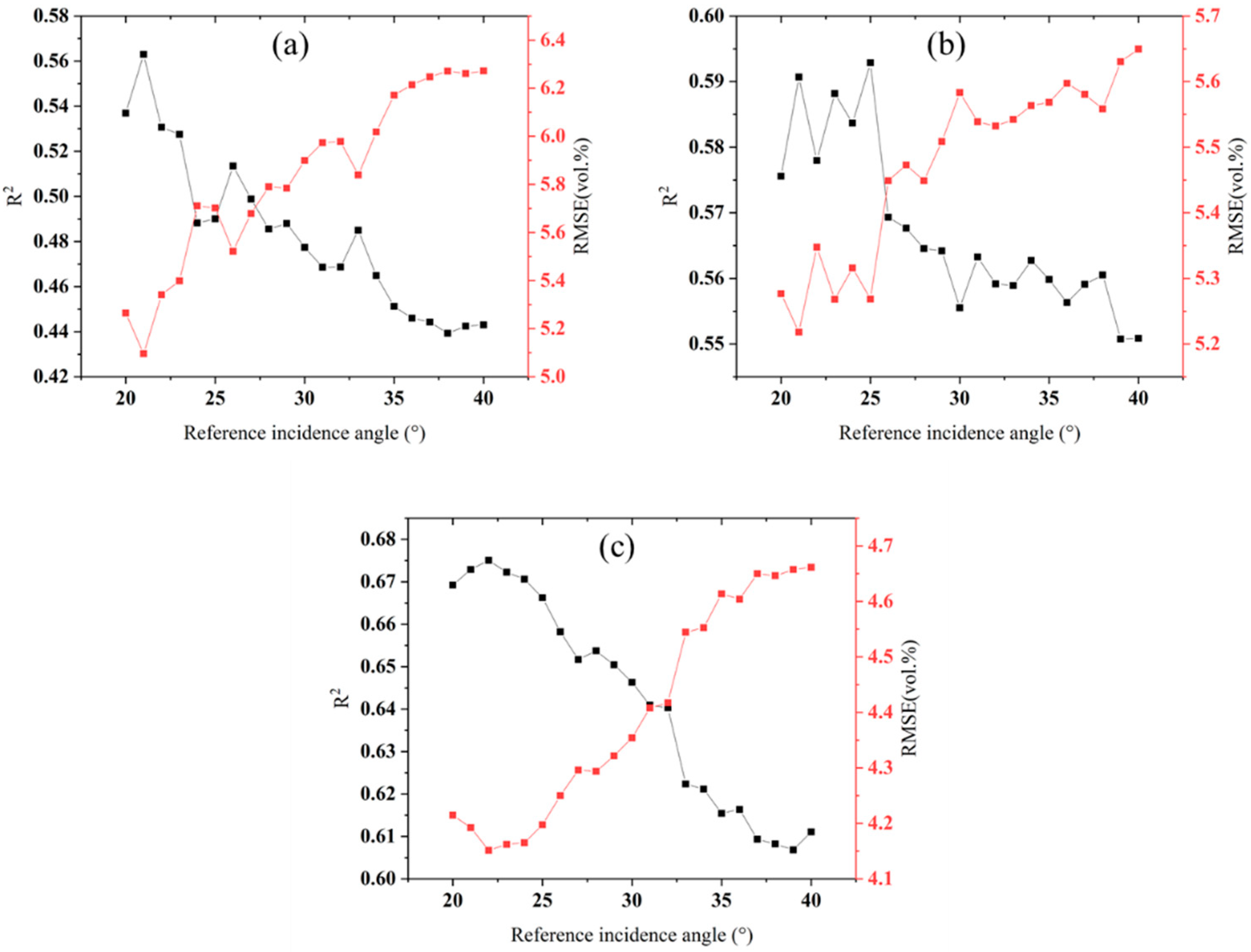
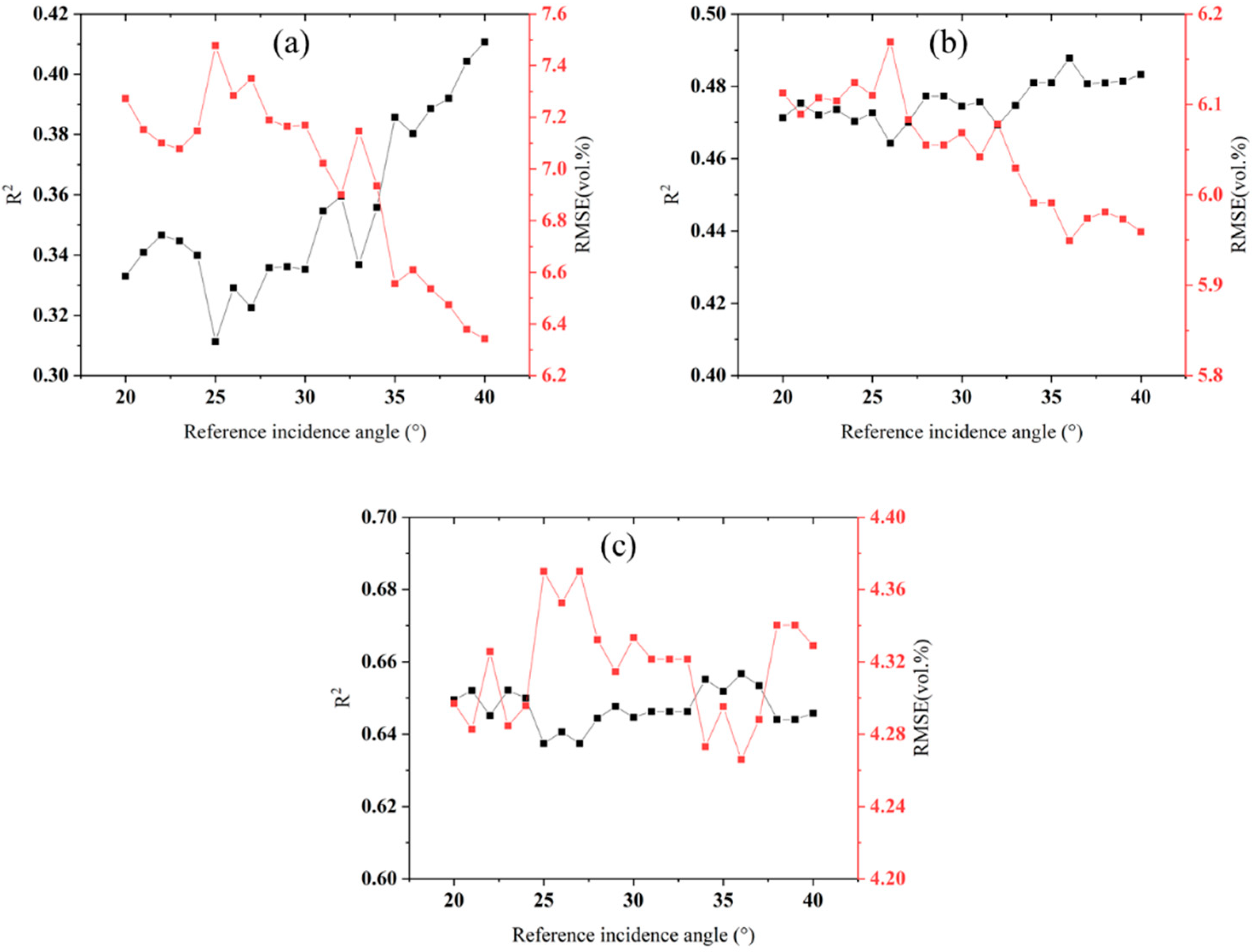
4.3. Reference Incidence Angle

The difference in distance between the ground object and the sensor would cause a difference in the incident angle, and the local incident angle would also be affected by the terrain. Since polarization signature can be affected by incidence angle, a normalization was performed at a reference incidence angle to reduce the effect of local incidence angle effect on the backscatter coefficients. In this study, the normalization method of incidence angle proposed by Ulaby et al. [41] was used to reduce the effect of local incidence angle on backscatter coefficients. The reference incidence angle was set to 30$°$. However, there was no unified conclusion on the selection of the reference incidence angle. In order to analyze the influence of the reference incidence angle on the estimation accuracy of the SMC estimation proposed in this study, the range of the reference incidence angle was 20$°$ to 40$°$, and the step size was set to 1$°$. The SMC on the validation set was retrieved by using the technical route constructed in Figure 3. When using different vegetation indices with different reference incidence angles, R² and RMSE between measured and estimated SMC values on the validation are shown in Figure 12 and Figure 13. The incidence angle corresponding to the minimum RMSE was taken as the optimal reference incidence angle.

Table 6. SMC estimation accuracy of validation when using the reference incidence angle.

Vegetation Correction Model	Vegetation Parameters	Reference Incidence Angle (°)	R2	RMSE (vol.%)
	RVI	21	0.56	5.10
Ratio method	LAI	22	0.59	5.22
	NDVI	21	0.68	4.15
	RVI	40	0.41	6.34
WCM	LAI	36	0.49	5.95
	NDVI	36	0.66	4.27

shows the SMC estimation accuracy of the validation set when the optimal reference incidence angle was used.

As shown in Figure 12, when estimating SMC based on the ratio method, the reference incidence angle had a significant impact on the SMC estimation results. The estimation accuracy on the validation set generally increased first and then decreased when the RVI, LAI, and NDVI served as vegetation descriptors. Meanwhile, it could be seen that, when RVI was used as vegetation descriptor, the variations in R² and RMSE curves are larger than that when the other two vegetation parameters were used. This may be due to the change of the simulated backscattering coefficients of the bare soil when the reference incidence angle changed. The RVI was also changed due to the influence of the normalization of the incidence angle. The parameters of dependent and independent variable changed when constructing the model. When LAI or NDVI serves as the descriptor, only the simulated backscattering coefficients of the bare soil changed, and the independent variable did not change. Therefore, when RVI was used as a vegetation description, RVI was more affected by the reference incidence angle than LAI or NDVI.

As shown in Table 5 and Table 6, the estimation accuracies of SMC were improved when using the optimal reference incident angle. Taking the ratio method combined with RVI as an example, it is known in the previous analysis that when the reference incident angle was 30$°$, the estimation performance based on RVI was the worst (R² = 0.48, RMSE = 5.90 vol.%). When using the optimal reference angle, the estimation accuracy of SMC was improved to R² = 0.56, RMSE = 5.10 vol.%. Therefore, when the models combined the optimal roughness parameter and the vegetation parameter for SMC retrieval, the reference incidence angle can also be used as another adjustment parameter to help improve the estimation accuracy.

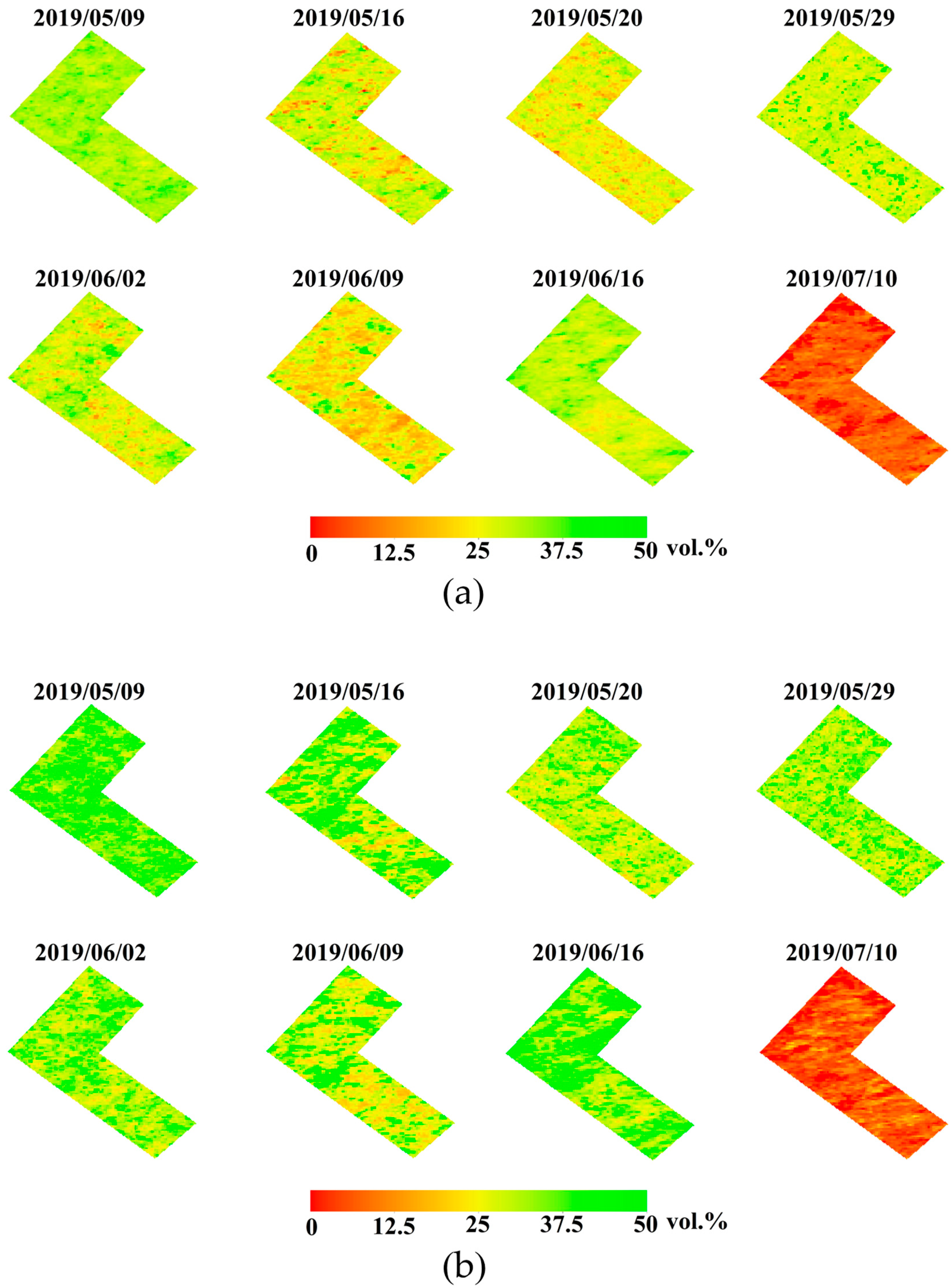
4.4. Regional Soil Moisture Mapping

In this study, LAI data were only available for a limited number of sampling points. Although NDVI could be extracted from optical images, it could not cover all sampling dates due to cloud interference in the study area. Therefore, only RVI was used as vegetation description parameter to construct the models for SMC mapping in this study. The SMC maps are shown in Figure 14. In general, the spatial patterns of the SMC maps obtained by the two models are consistent, and they conform to the trend of the measured SMC throughout the growing season. Comparing Figure 14a,b, the soil moisture values retrieved by WCM are higher in the area with high SMC, reaching the critical value of 50 vol.% in most areas, which shows an apparent overestimation compared with the measured soil moisture. In contrast, there is no obvious overestimation area in the SMC map based on the ratio method. On the last sampling date, both models showed an obvious underestimation. This is mainly because the SMC measured on July 10 was low, and the CIEM model is not sensitive to soil changes when the SMC is low.

4.5. Limitations and Potential Improvements

Due to various constrains, soil moisture measurements did not cover the entire wheat growing season in this study. Further experiments can be conducted in the future to collect and analyze soil moisture information for the whole growing season of wheat to evaluate the effectiveness and applicability of the method proposed in this study. The effectiveness of the proposed methods for other crop types is also worth further verification in future studies.

From a spatial coverage point of view, the study area in this study was limited to a single wheat field, so the optimal roughness parameter was used to characterize the roughness condition of the whole study area. When conducting soil moisture inversion over a large agricultural area, the root-mean-square height or correlation length of the surface can be obtained by inverting the surface roughness, which and then be used to construct an improved surface scattering model.

5. Conclusions

In this study, based on RADARSAT-2 SAR data and the measured SMC information, we investigated the potential of a simple method combined with three different vegetation parameters to estimate SMC under vegetation cover. In addition, the WCM was also used to retrieve SMC for comparison. Based on the study, the following conclusions can be drawn:

(1)

As an empirical coefficient in the scattering model, the optimal roughness parameter could effectively improve the estimation accuracy of SMC.

(2)

A reference incident angle could be used as an effective adjustment parameter to improve the estimation accuracy of SMC.

(3)

Comparing with LAI and RVI, NDVI is more suitable as the vegetation description parameter of the model.

(4)

In general, the estimation performance of the ratio method is better than that of WCM.

Despite the encouraging results of this study, there are certain limitations that need to be addressed in future studies. The measured data in this study only covered part of the wheat growing period. In the future, it will be necessary to evaluate the effectiveness of the proposed method over longer wheat growth cycles. In addition, the same method should be tested on other crop types to further verify its effectiveness.

References

1. Lievens, H.; Vernieuwe, H.; Alvarez-Mozos, J.; De Baets, B.; Verhoest, N.E. Error in radar-derived soil moisture due to roughness parameterization: An analysis based on synthetical surface profiles. Sensors 2009, 9, 1067–1093. [Google Scholar] [CrossRef] [PubMed] [Green Version]
2. Wang, S.; Li, X.; Han, X.; Jin, R. Estimation of surface soil moisture and roughness from multi-angular ASAR imagery in the Watershed Allied Telemetry Experimental Research (WATER). Hydrol. Earth Syst. Sci. 2011, 15, 1415–1426. [Google Scholar] [CrossRef] [Green Version]
3. Prakash, R.; Singh, D.; Pathak, N.P. A fusion approach to retrieve soil moisture with SAR and optical data. IEEE J.-Stars 2011, 5, 196–206. [Google Scholar] [CrossRef]
4. De Keyser, E.; Vernieuwe, H.; Lievens, H.; Álvarez-Mozos, J.; De Baets, B.; Verhoest, N.E. Assessment of SAR-retrieved soil moisture uncertainty induced by uncertainty on modeled soil surface roughness. Int. J. Appl. Earth Obs. Geoinf. 2012, 18, 176–182. [Google Scholar] [CrossRef]
5. Bao, Y.; Zhang, Y.; Wang, J.; Min, J. Surface soil moisture estimation over dense crop using Envisat ASAR and Landsat TM imagery: An approach. Int. J. Remote Sens. 2014, 35, 6190–6212. [Google Scholar] [CrossRef]
6. Li, Z.-L.; Leng, P.; Zhou, C.; Chen, K.-S.; Zhou, F.-C.; Shang, G.-F. Soil moisture retrieval from remote sensing measurements: Current knowledge and directions for the future. Earth-Sci. Rev. 2021, 218, 103673. [Google Scholar] [CrossRef]
7. Gao, Z.; Xu, X.; Wang, J.; Yang, H.; Huang, W.; Feng, H. A method of estimating soil moisture based on the linear decomposition of mixture pixels. Math. Comput. Model. 2013, 58, 606–613. [Google Scholar] [CrossRef]
8. Haubrock, S.N.; Chabrillat, S.; Lemmnitz, C.; Kaufmann, H. Surface soil moisture quantification models from reflectance data under field conditions. Int. J. Remote Sens. 2008, 29, 3–29. [Google Scholar] [CrossRef]
9. Liu, W.; Baret, F.; Gu, X.; Zhang, B.; Tong, Q.; Zheng, L. Evaluation of methods for soil surface moisture estimation from reflectance data. Int. J. Remote Sens. 2003, 24, 2069–2083. [Google Scholar] [CrossRef]
10. Engstrom, R.; Hope, A.; Kwon, H.; Stow, D. The relationship between soil moisture and NDVI near Barrow, Alaska. Phys. Geogr. 2008, 29, 38–53. [Google Scholar] [CrossRef]
11. Schnur, M.T.; Xie, H.; Wang, X. Estimating root zone soil moisture at distant sites using MODIS NDVI and EVI in a semi-arid region of southwestern USA. Ecol. Inform. 2010, 5, 400–409. [Google Scholar] [CrossRef]
12. Zribi, M.; Paris Anguela, T.; Duchemin, B.; Lili, Z.; Wagner, W.; Hasenauer, S.; Chehbouni, A. Relationship between soil moisture and vegetation in the Kairouan plain region of Tunisia using low spatial resolution satellite data. Water Resour. Res. 2010, 46, W06508. [Google Scholar] [CrossRef] [Green Version]
13. Chang, T.-Y.; Wang, Y.-C.; Feng, C.-C.; Ziegler, A.D.; Giambelluca, T.W.; Liou, Y.-A. Estimation of root zone soil moisture using apparent thermal inertia with MODIS imagery over a tropical catchment in Northern Thailand. IEEE J.-Stars 2012, 5, 752–761. [Google Scholar] [CrossRef]
14. Matsushima, D.; Kimura, R.; Shinoda, M. Soil moisture estimation using thermal inertia: Potential and sensitivity to data conditions. J. Hydrometeorol. 2012, 13, 638–648. [Google Scholar] [CrossRef]
15. Minacapilli, M.; Cammalleri, C.; Ciraolo, G.; D’Asaro, F.; Iovino, M.; Maltese, A. Thermal inertia modeling for soil surface water content estimation: A laboratory experiment. Soil Sci. Soc. Am. J. 2012, 76, 92–100. [Google Scholar] [CrossRef]
16. Bindlish, R.; Jackson, T.; Gasiewski, A.; Stankov, B.; Klein, M.; Cosh, M.; Mladenova, I.; Watts, C.; Vivoni, E.; Lakshmi, V. Aircraft based soil moisture retrievals under mixed vegetation and topographic conditions. Remote Sens. Environ. 2008, 112, 375–390. [Google Scholar] [CrossRef]
17. Yan, F.; Qin, Z.; Li, M.; Li, W. Progress in soil moisture estimation from remote sensing data for agricultural drought monitoring. Remote Sens. Environ. Monit. GIS Appl. Geol. VI 2006, 6366, 636601. [Google Scholar]
18. Zhang, D.; Zhou, G. Estimation of soil moisture from optical and thermal remote sensing: A review. Sensors 2016, 16, 1308. [Google Scholar] [CrossRef] [Green Version]
19. Bhogapurapu, N.; Dey, S.; Mandal, D.; Bhattacharya, A.; Karthikeyan, L.; McNairn, H.; Rao, Y. Soil moisture retrieval over croplands using dual-pol L-band GRD SAR data. Remote Sens. Environ. 2022, 271, 112900. [Google Scholar] [CrossRef]
20. Chen, L.; Xing, M.; He, B.; Wang, J.; Shang, J.; Huang, X.; Xu, M. Estimating soil moisture over winter wheat fields during growing season using machine-learning methods. IEEE J.-Stars 2021, 14, 3706–3718. [Google Scholar] [CrossRef]
21. Xing, M.; He, B.; Ni, X.; Wang, J.; An, G.; Shang, J.; Huang, X. Retrieving surface soil moisture over wheat and soybean fields during growing season using modified water cloud model from Radarsat-2 SAR data. Remote Sens. 2019, 11, 1956. [Google Scholar] [CrossRef] [Green Version]
22. Srivastava, H.S.; Patel, P.; Sharma, Y.; Navalgund, R.R. Large-area soil moisture estimation using multi-incidence-angle RADARSAT-1 SAR data. IEEE Trans. Geosci. Remote Sens. 2009, 47, 2528–2535. [Google Scholar] [CrossRef]
23. Lakhankar, T.; Ghedira, H.; Temimi, M.; Azar, A.E.; Khanbilvardi, R. Effect of land cover heterogeneity on soil moisture retrieval using active microwave remote sensing data. Remote Sens. 2009, 1, 80–91. [Google Scholar] [CrossRef] [Green Version]
24. Sang, H.; Zhang, J.; Lin, H.; Zhai, L. Multi-polarization ASAR backscattering from herbaceous wetlands in Poyang Lake region, China. Remote Sens. 2014, 6, 4621–4646. [Google Scholar] [CrossRef] [Green Version]
25. Xiao, T.; Xing, M.; He, B.; Wang, J.; Shang, J.; Huang, X.; Ni, X. Retrieving Soil Moisture Over Soybean Fields During Growing Season Through Polarimetric Decomposition. IEEE J.-Stars 2020, 14, 1132–1145. [Google Scholar] [CrossRef]
26. Gherboudj, I.; Magagi, R.; Berg, A.A.; Toth, B. Soil moisture retrieval over agricultural fields from multi-polarized and multi-angular RADARSAT-2 SAR data. Remote Sens. Environ. 2011, 115, 33–43. [Google Scholar] [CrossRef]
27. Notarnicola, C.; Angiulli, M.; Posa, F. Use of radar and optical remotely sensed data for soil moisture retrieval over vegetated areas. IEEE Trans. Geosci. Remote Sens. 2006, 44, 925–935. [Google Scholar] [CrossRef]
28. Bolten, J.D.; Lakshmi, V.; Njoku, E.G. Soil moisture retrieval using the passive/active L-and S-band radar/radiometer. IEEE Trans. Geosci. Remote Sens. 2003, 41, 2792–2801. [Google Scholar] [CrossRef]
29. Chen, L.; Xing, M.F.; He, B.B.; Wang, J.F.; Xu, M.; Song, Y.; Huang, X.D. Estimating Soil Moisture over Winter Wheat Fields during Growing Season Using RADARSAT-2 Data. Remote Sens. 2022, 14, 2232. [Google Scholar] [CrossRef]
30. Wang, Z.; Zhao, T.; Qiu, J.; Zhao, X.; Wang, S. Microwave-based vegetation descriptors in the parameterization of water cloud model at L-band for soil moisture retrieval over croplands. Gisci. Remote Sens. 2020, 58, 48–67. [Google Scholar] [CrossRef]
31. Hajnsek, I.; Jagdhuber, T.; Schon, H.; Papathanassiou, K.P. Potential of Estimating Soil Moisture Under Vegetation Cover by Means of PolSAR. IEEE Trans. Geosci. Remote Sens. 2009, 47, 442–454. [Google Scholar] [CrossRef] [Green Version]
32. Jagdhuber, T.; Hajnsek, I.; Bronstert, A.; Papathanassiou, K.P. Soil Moisture Estimation Under Low Vegetation Cover Using a Multi-Angular Polarimetric Decomposition. IEEE Trans. Geosci. Remote Sens. 2013, 51, 2201–2215. [Google Scholar] [CrossRef]
33. Martino, G.D.; Iodice, A.; Natale, A.; Riccio, D. Polarimetric Two-Scale Two-Component Model for the Retrieval of Soil Moisture Under Moderate Vegetation via L-Band SAR Data. IEEE Trans. Geosci. Remote Sens. 2016, 54, 2470–2491. [Google Scholar] [CrossRef]
34. Ulaby, F.T.; Sarabandi, K.; Mcdonald, K.; Whitt, M.; Dobson, M.C. Michigan microwave canopy scattering model. Int. J. Remote Sens. 1990, 11, 1223–1253. [Google Scholar] [CrossRef]
35. Attema, E.; Ulaby, F.T. Vegetation modeled as a water cloud. Radio Sci. 1978, 13, 357–364. [Google Scholar] [CrossRef]
36. Lang, R.H.; Sighu, J.S. Electromagnetic Backscattering From a Layer of Vegetation: A Discrete Approach. IEEE Trans. Geosci. Remote Sens. 1983, GE-21, 62–71. [Google Scholar] [CrossRef]
37. Ferrazzoli, P.; Guerriero, L. Emissivity of vegetation: Theory and computational aspects. J. Electromagn. Waves Appl. 1996, 10, 609–628. [Google Scholar] [CrossRef]
38. Liao, C.; Wang, J.; Ian, P.; Liu, J.; Shang, J. A Spatio-Temporal Data Fusion Model for Generating NDVI Time Series in Heterogeneous Regions. Remote Sens. 2017, 9, 1125. [Google Scholar] [CrossRef] [Green Version]
39. Lievens, H.; Verhoest, N.E. On the retrieval of soil moisture in wheat fields from L-band SAR based on water cloud modeling, the IEM, and effective roughness parameters. IEEE Geosci. Remote Sens. Lett. 2011, 8, 740–744. [Google Scholar] [CrossRef]
40. Baghdadi, N.; Holah, N.; Zribi, M. Calibration of the Integral Equation Model for SAR data in C-band and HH and VV polarizations. Int. J. Remote Sens. 2006, 27, 805–816. [Google Scholar] [CrossRef]
41. Ulaby, F.T.; Moore, R.K.; Fung, A.K. Microwave Remote Sensing: Active and Passive, V.2: Radar Remote Sensing and Surface Scattering and Emission Theory; Addison-Wesley Pub. Co. Advanced Book Program/World Science Division: Reading, MA, USA, 1982. [Google Scholar]
42. Long, W.; Quan, X.; He, B.; Yebra, M.; Liu, X.J.R.S. Assessment of the Dual Polarimetric Sentinel-1A Data for Forest Fuel Moisture Content Estimation. Remote Sens. 2019, 11, 1568. [Google Scholar]
43. Joseph, A.T.; van der Velde, R.; O’Neill, P.E.; Lang, R.H.; Gish, T. Soil Moisture Retrieval During a Corn Growth Cycle Using L-Band (1.6 GHz) Radar Observations. IEEE Trans. Geosci. Remote Sens. 2008, 46, 2365–2374. [Google Scholar] [CrossRef] [Green Version]
44. Joseph, A.T.; van der Velde, R.; O’Neill, P.E.; Lang, R.; Gish, T. Effects of corn on C- and L-band radar backscatter: A correction method for soil moisture retrieval. Remote Sens. Environ. 2010, 114, 2417–2430. [Google Scholar] [CrossRef]
45. Bai, X.J.; He, B.B.; Xing, M.F.; Li, X.W. Method for soil moisture retrieval in arid prairie using TerraSAR-X data. J. Appl. Remote Sens. 2015, 9, 096062. [Google Scholar] [CrossRef]
46. Mironov, V.L.; Dobson, M.C.; Kaupp, V.H.; Komarov, S.A.; Kleshchenko, V.N. Generalized refractive mixing dielectric model for moist soils. IEEE Trans. Geosci. Remote Sens. 2004, 42, 773–785. [Google Scholar] [CrossRef]
47. Kseneman, M.; Gleich, D. Soil-Moisture Estimation From X-Band Data Using Tikhonov Regularization and Neural Net. IEEE Trans. Geosci. Remote Sens. 2013, 51, 3885–3898. [Google Scholar] [CrossRef]
48. Fung, A.K.; Li, Z.Q.; Chen, K.S. Backscattering From a Randomly Rough Dielectric Surface. IEEE Trans. Geosci. Remote Sens. 1992, 30, 356–369. [Google Scholar] [CrossRef]
49. Bryant, R.; Moran, M.S.; Thoma, D.P.; Collins, C.H.; Skirvin, S.; Rahman, M.; Slocum, K.; Starks, P.; Bosch, D.; Dugo, M.G. Measuring Surface Roughness Height to Parameterize Radar Backscatter Models for Retrieval of Surface Soil Moisture. IEEE Geosci. Remote Sens. Lett. 2007, 4, 137–141. [Google Scholar] [CrossRef]
50. Bai, X.J.; He, B.B.; Li, X.W. Optimum Surface Roughness to Parameterize Advanced Integral Equation Model for Soil Moisture Retrieval in Prairie Area Using Radarsat-2 Data. IEEE Trans. Geosci. Remote Sens. 2016, 54, 2437–2449. [Google Scholar] [CrossRef]
Figure 1. Location of the study area.
Remotesensing 14 03210 g001
Figure 2. Ground truth photos of winter wheat. (a) 9 May. (b) 27 May. (c) 9 June. (d) 10 July 2019.
Remotesensing 14 03210 g002
Figure 3. Workflow of soil moisture retrieval.
Remotesensing 14 03210 g003
Figure 4. SMC estimation accuracy on the training set with different roughness parameters (Ratio method), (a) 9 May, (b) 16 May, (c) 20 May, (d) 29 May, (e) 2 June, (f) 9 June, (g) 16 June, (h) 10 July in 2019.
Remotesensing 14 03210 g004
Figure 5. SMC estimation accuracy on training set with different roughness parameters (WCM), (a) 9 May, (b) 16 May, (c) 20 May, (d) 29 May, (e) 2 June, (f) June, (g) 16 June, (h) 10 July in 2019.
Remotesensing 14 03210 g005aRemotesensing 14 03210 g005b
Figure 6. Scatterplots between the measured and predicted SMC values on the validation set based on RVI (Ratio method).
Remotesensing 14 03210 g006
Figure 7. (a) Scatterplots between the measured and predicted SMC values on the validation set based on LAI (Ratio method); (b) scatterplots between the measured and predicted SMC values on the validation set based on RVI, the same date as LAI (Ratio method).
Remotesensing 14 03210 g007
Figure 8. (a) Scatterplots between the measured and predicted SMC values on the validation set based on NDVI (Ratio method); (b) scatterplots between the measured and predicted SMC values on the validation set based on RVI, the same date as NDVI (Ratio method).
Remotesensing 14 03210 g008
Figure 9. Scatterplots between the measured and predicted SMC values on the validation set based on RVI (WCM).
Remotesensing 14 03210 g009
Figure 10. (a) Scatterplots between the measured and predicted SMC values on the validation set based on LAI (WCM); (b) scatterplots between the measured and predicted SMC values on the validation set based on RVI, the same date as LAI (WCM).
Remotesensing 14 03210 g010
Figure 11. (a) Scatterplots between the measured and predicted SMC values on the validation set based on NDVI (WCM); (b) scatterplots between the measured and predicted SMC values on the validation set based on RVI, the same date as NDVI (WCM).
Remotesensing 14 03210 g011
Figure 12. SMC estimation accuracy based on ratio method with different reference incidence angels. (a) RVI; (b) LAI; (c) NDVI.
Remotesensing 14 03210 g012
Figure 13. SMC estimation accuracy based on WCM with different reference incidence angels. (a) RVI; (b) LAI; (c) NDVI.
Remotesensing 14 03210 g013
Figure 14. Soil moisture maps of the study area; (a) Ratio method; (b) WCM.
Remotesensing 14 03210 g014