Abstract
In Mars exploration, hyper-spectrometry plays an important role due to its high spectral resolution. However, due to the technical difficulty and the data size, the spatial resolution or the coverage of hyperspectral data is often limited. This limitation can be alleviated by deep learning-based super-resolution (SR) reconstruction. But the spatial size and batch size of the input training data is limited due to the large number of spectral channels. To improve the efficiency of model training and SR reconstruction, a dataset based on CRISM hyperspectral data is created in this paper, and its redundancy is analyzed in both spectral and spatial spital dimensions. Compression algorithms based on data selection and PCA are used to reduce the size of the input training data. A network that can perform spatial SR and spectral enhancement is also proposed to make the network can be trained with the compressed data. With these compression algorithms and network, high-resolution data with 235 bands can be reconstructed from the low-resolution data with only 40 bands. Compared with the network trained on the original low-resolution data with 235 bands, the model training time and the SR reconstruction runtime can be reduced to 30% and 23% with practically no accuracy loss. The effectiveness of compression algorithms based on data selection also indicates that maybe not all the bands need to be transmitted from the Mars probes or be collected. Furthermore, it would, in principle, help improve the efficiency of satellite data transmission and simplify the design of the hyper-spectrometer. Additionally, a method for spatial dimension correlation evaluation is also proposed in this paper. The spatial compression shows that the proposed method can reflect the correlation of spatial texture between patches, and the model can be acceptably trained with only half of the original data.
1. Introduction
Mars exploration started in the 1960s with the successful launch of humanity’s first Mars probe [1,2]. Since then, about fifty Mars exploration satellites have been launched over the past six decades, revealing people’s enthusiasm for Mars exploration [3]. Since Mars is the most Earth-like planet in the solar system, the study of Mars can help human beings understand the long-term evolution of the Earth [4,5,6]. Martian research includes climate and environmental evolution [7,8,9],topography and geomorphology research [10,11], Martian surface composition analysis [12,13], and water detection [14,15], etc.
In remote sensing instruments, hyper-spectrometers play an important role in the material composition analysis of Mars due to their high spectral resolution and the ability to detect spatial and spectral features synchronously. Some of the Mars hyper-spectrometers and their specifications are listed in Table 1 [16,17]. With the rich spectral information, hyperspectral data collected by hyper-spectrometers can be used for quantitative remote sensing [18,19]. It is often difficult for the remote sensing data to provide high resolution in both the spatial dimension and spectral dimension at the same time due to the technical challenges, the manufacturing cost of the hyper-spectrometer, and the large size of data. So, most Martian hyperspectral data have a spatial resolution of tens to hundreds of meters. Although the spatial resolution of some hyperspectral data, such as the CRISM FRT data, can reach 18m, its coverage is limited. When the spatial resolution is low, the obtained spectral features of ground objects are mixed, and the detection accuracy is reduced [20]. Therefore, it is impossible to do a global high-precision Martian surface composition analysis. Thus, it is of great significance to improve the spatial resolution of hyperspectral remote sensing data. It will be helpful to make a more accurate analysis of the mineral and water-ice distribution in the Martian gullies, deltas, alluvial fans, dry river beds, and ditches globally.

Table 1.
Some of the Mars hyper-spectrometer and their specifications.
The primary technique for improving the spatial resolution of hyperspectral images is image super-resolution (SR) reconstruction. The SR reconstruction algorithms can be classified into three types: image interpolation [21,22], image reconstruction [23], and deep learning-based reconstruction [24,25,26,27]. The image interpolation algorithms are simple, but details are easily lost in the reconstruction results. The image reconstruction methods have the advantages of low computational cost and fast convergence speed, but their performance is still unsatisfactory. SR reconstruction algorithms based on deep learning have been intensely studied in recent years. With the rapid development of deep learning, these algorithms show better performance and continuous improvement potential. Additionally, reliant on whether there is auxiliary information (e.g., high spatial resolution RGB or panchromatic images), the SR reconstruction algorithms can be classified into fusion-based SR and single SR [28,29]. In the fusion-based SR, the auxiliary information is indispensable. Being hard to obtain good co-registered auxiliary images on Mars, single SR algorithms are the best choice for the SR of Mars hyperspectral data.
The essence of the SR algorithm is the mapping function between the low-resolution and high-resolution data. Deep learning-based algorithms can construct complex nonlinear mapping functions through multi-layer neural networks and activation functions. Meanwhile, backpropagation and optimized gradient descent algorithms enable deep learning to autonomously learn the mapping relationship between input and output data. Therefore, deep learning has been widely used in various algorithms. In image processing, the introduction of the convolutional neural network simplifies the network significantly due to its local connection and weight sharing, making it much easier to train and deploy. Therefore, deep learning was first introduced into SR reconstruction in a network named SR Convolutional Neural Network (SRCNN) in 2014 [30]. Subsequently, the residual network was also introduced into SR algorithms due to its shortcut structure, which can solve the degradation problem and make deeper learning possible [31,32]. Different from the RGB data, there are dozens or even hundreds of channels in the spectral dimension of hyperspectral images. The accuracy of spectral information determines the value of hyperspectral data directly. Therefore, it is essential to preserve the spectral information of hyperspectral data well while enhancing its spatial information, and spatial loss and spectral loss are combined to drive the learning of the SR network [33,34,35]. In addition, due to its high resolution in the spectral dimension, the size of the hyperspectral data is much larger than the RGB data. It makes the SR networks of hyperspectral data more complex and more difficult to train. To simplify the network structure and improve training efficiency, branch networks began to appear in the hyperspectral SR network [36]. Hyperspectral data are divided into several groups and fed to different branch networks for spatial-spectral feature extraction. The features of these branch networks will then be merged into the back of the network for global information learning. In the spatial-spectral prior network-based SR network (SSPSR), the parameters of the branch networks are shared and improve training efficiency further [37].
For all models mentioned above, the whole bands of the hyperspectral data need to be fed to the network. It limits the spatial size and batch size of the input training data and lengthens the model training and SR reconstruction time significantly. The types of Martian surface materials are much less than the pixel number of the hyperspectral data, the spectral curve of these materials is continuous, and due to the high resolution of the hyperspectral data the difference in the central wavelength between adjacent spectral segments is very small. Therefore, the redundancy between these bands may be quite high, and the size of the input data may be significantly compressed while retaining most of the information. If the SR network can be trained well with the compressed data, the model training and SR reconstruction time may be reduced significantly. To verify its feasibility, a dataset based on Compact Reconnaissance Imaging Spectrometer for Mars (CRISM) hyperspectral remote sensing data is created in this paper, and its redundancy is analyzed in detail in both spectral and spatial dimensions. Compression algorithms based on data selection are proposed for reducing the size of the input training data. A network that can perform both spatial SR and spectral enhancement simultaneously is also proposed in this paper to make the network can be trained with the compressed data.
2. Materials
2.1. Data Description
The Compact Reconnaissance Imaging Spectrometer for Mars (CRISM) onboard the Mars Reconnaissance Orbiter (MRO) is a hyperspectral imager for Mars exploration. It has three major types of observations. In multispectral mapping (MSP) mode, data are collected at a subset of 72 wavelengths covering the key mineralogic absorptions and binned to pixel footprints of 100 or 200 m/pixel. In full resolution targeted (FRT) mode, a region of interest is mapped at full spatial and spectral resolution (15–19 m/pixel, 362–3920 nm at 6.55 nm/channel). In atmospheric mode, only the emission phase function(EPF) is acquired [38]. The MRO has returned more data than all previous Mars missions combined. As of early 2022, it continues to send high-resolution data of Mars features and weather [3]. Besides, due to its high spatial and spectral resolution, CRISM collected in FRT mode is selected as the experimental data in this paper. Considering the mineral spectral features range and avoiding the interference of thermal emission, the data in the wavelength range of 1.1 μm–2.65 μm are selected to build the dataset for model training and testing. The number of the selected bands is 235, and the product IDs of the selected CRISM data are listed in Table A1.
2.2. Dataset Creation
2.2.1. Data Pre-Processing
The pre-processing of the selected CRISM data can be performed by ENVI with a plug-in called CRISM Analysis Toolkit (CAT) [39]. The plug-in is developed by the CRISM scientific team for CRISM data processing and analysis. The pre-processing of CRISM data includes the following steps. (1) Photometric and atmospheric correction. In the atmospheric correction, the Martian atmospheric absorption, scattering, and reflection effects on the spectrum are eliminated, and the actual reflectance of the Martian surface is obtained [40]. In the photometric correction, the image reflectance differences caused by the change of solar altitude angle will be removed. (2) Stripes and speckle noise removal. This step eliminates the influence of the environment and the spectrometer during data acquisition. (3) Geometric correction. The map projection will be completed to match the geographic coordinates in this step. (4) Invalid data imputation.
2.2.2. Data Cropping
Six of the fifty-seven pre-processed CRISM data were selected randomly as test data, another six data were selected randomly as validation data, and the other forty-five data were selected as training data. The indexes of the test data are 1, 27, 29, 27, 43, and 51. The indexes of the validation data are 4, 13, 20, 32, 52, and 53. Please refer to Table A1 for the corresponding relationship between these indexes and the product IDs of the selected data. For each test data, a 512 × 512 rectangular region was cropped, and then the six rectangular data were stacked together. Thus, the size of the test data is 6 × 512 × 512 × 235. For training and validation data, a rectangular region was cropped as large as possible in each data. Then 64 × 64 patches were cropped from these rectangular regions, and the stride in both the height and width direction is 32. The low-resolution patches are obtained by bicubic downsampling these patches, and the downsampling factor is 4. At last, there are 1376 patches in the validation dataset and 10,713 patches in the training dataset. Therefore, the spatial resolution of the input low-resolution training and validation data is 16 × 16, and the spatial resolution of the input low-resolution test data is 128 × 128.
3. Method
3.1. Hyperspectral Image SR Algorithm
The hyperspectral image SR algorithm used in this paper is modified based on the SSPSR [37]. Compared with SSPSR, the channel numbers of the low-resolution image and the high-resolution output image are defined independently, and the network is modified accordingly. Thus, the modified network can perform not only spatial SR but also spectral enhancement, and the modified network can output high-resolution hyperspectral images based on low-resolution images with fewer spectral bands. Please refer to Appendix B for the detailed description of the SSPSR network and the model training parameters configuration.
3.2. Data Compression Algorithms
Each patch of the created CRISM dataset has three dimensions: length, width, and band. The length and width correspond to the spatial dimension, and the band corresponds to the spectral dimension. Therefore, data compression can be carried out from the spectral and spatial dimensions.
Compression algorithms based on data selection proposed in this paper and based on principal component analysis (PCA) are used for data compression.
3.2.1. Spectral Compression
- Compression Algorithms Based on Data Selection
For compression algorithms based on data selection, the correlation coefficients of the specified dimension between low-resolution training data are calculated. When the correlation coefficient exceeds the set threshold, one of the two data will be removed. The correlation coefficient mentioned in this paper refers to Pearson Correlation Coefficient. If data A and B have N scalar observations, then the Pearson Correlation Coefficient is defined as:
where and are the mean and standard deviation of , respectively, and and are the mean and standard deviation of .
When the data are compressed in spectral dimension, a set of selected bands must be found first. For each band in this set, the correlation coefficient between this band and the other bands in the set should be less than the set threshold. For each band that is not contained in the set, there should be at least one band in the set to make the correlation coefficient between them greater than or equal to the set threshold. When the selected bands are found, the data of the corresponding bands will be retained in low-resolution data, and the data of the other bands in low-resolution data will be removed. All bands of the ground truth will be retained.
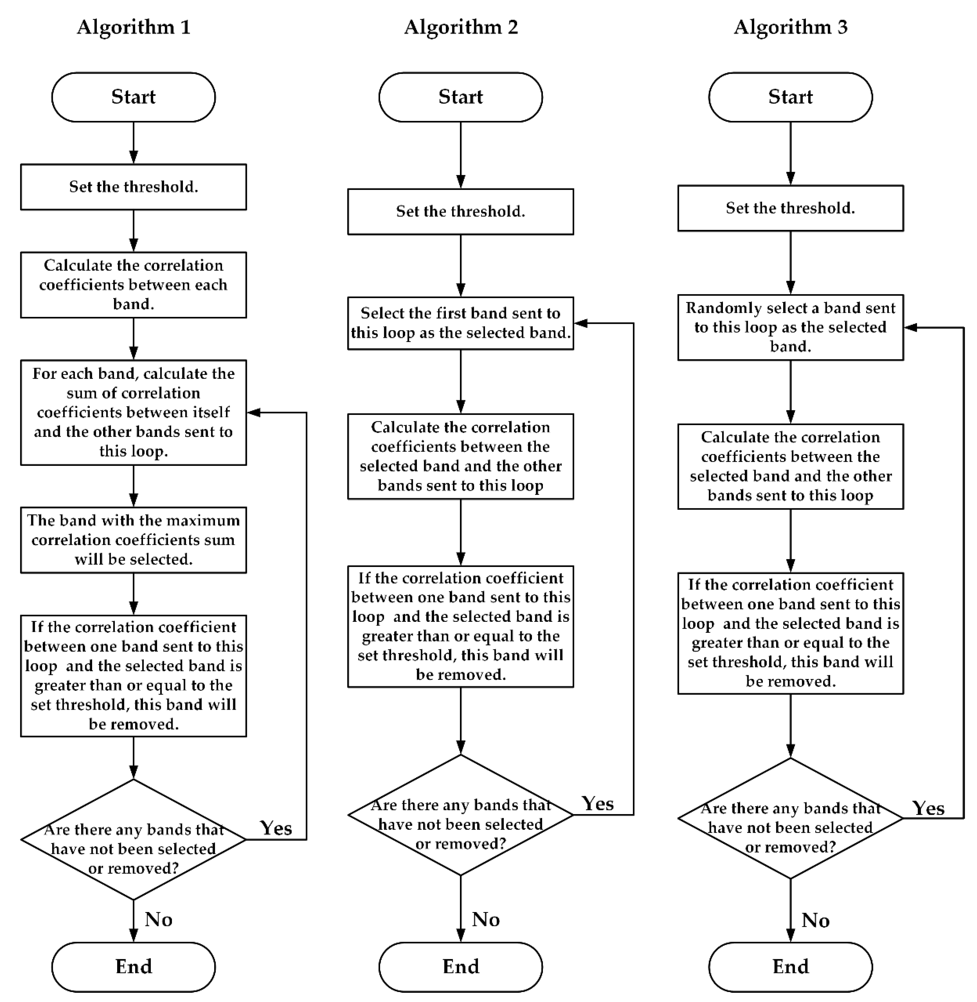
To find the selected bands, three algorithms were proposed. The workflow charts of the three algorithms are presented in Figure 1.
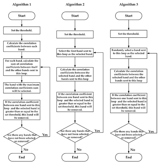
Figure 1.
The workflow charts of the three compression algorithms based on data selection.
In Algorithm 1, all the correlation coefficients between each band are calculated first. Then, the sum of correlation coefficients between this band and the other bands will be calculated for each band. The band with the maximum correlation coefficients sum will be selected. For the other bands, if the correlation coefficient between one band and the selected band is greater than or equal to the set threshold, this band will be removed. Bands not selected or removed will be sent to the next loop. In the next loop, for each band, the sum of correlation coefficients between this band and other bands sent to this loop will be calculated, another band will be selected, and some bands will be removed as in the previous loop. If there are still some bands that have not been selected or removed, these bands will be sent to the next loop. At last, all the selected bands will be found.
In Algorithm 2, the first band will be selected first. And then, the correlation coefficients between the selected and other bands will be calculated. If the correlation coefficient between one band and the selected band is greater than or equal to the set threshold, this band will be removed. Bands not selected or removed will be sent to the next loop. The first band of this loop will also be selected, then the correlation coefficients between the selected band and the other bands sent to this loop will be calculated. If the correlation coefficient between one band and the selected band is greater than or equal to the set threshold, this band will be removed in this loop. If there are still some bands that have not been selected or removed, these bands will be sent to the next loop. Finally, all the selected bands will be found.
It can be found that correlation coefficients between all bands need to be calculated in Algorithm 1. However, in Algorithm 2, only correlation coefficients between the selected and the other bands in the current loop must be calculated. Besides, for algorithm 2, due to the data’s continuity in spectral dimension, many bands with high correlation coefficients with the first band had been selected or removed already. It will lead to a decrease in operational efficiency. To solve this problem, the selected band in each loop can be selected randomly; Algorithm 3.
- 2.
- Compression Algorithm Based on PCA
The PCA algorithm is a widely used data dimensionality reduction algorithm in deep learning [41,42,43]. The central idea of PCA is to reduce the dimensionality of a data set consisting of many interrelated variables while retaining as much as possible of the variation present in the data set, which is achieved by transforming the original data into a new set of variables. The principal components are uncorrelated and ordered so that the first few retain most of the variation present in all of the original variables [44]. For the compression algorithm based on PCA, the covariance matrix of the 235 bands data is calculated first. Then the eigenvectors and eigenvalues of the covariance matrix are calculated. The eigenvectors are sorted in descending order according to their corresponding eigenvalues. The proportion of variation explained by each eigenvalue is used to evaluate the contribution rate of each eigenvalue. Finally, according to the required contribution rate or the number of principal components, eigenvectors corresponding to the largest n eigenvalues are selected to form a 235 × n transformation matrix U. The compressed data of each pixel will be obtained by multiplying the column vector formed by the data of the original 235 bands with the transformation matrix U.
3.2.2. Spatial Compression
In spatial compression, the quantity of patches is usually a large number. For example, the quantity of the training patches used in this paper is 10,713. It means that both the conversion matrix solving and the data conversion need a lot of floating-point operations. Besides, in spectral compression, the bands for a specific data source are relatively fixed, while the patches may be changed with the accumulation of the remote sensing data. When the dataset changes, the transformation matrix and the compressed data need to be regenerated, which means the extensibility of the PCA algorithm is not sufficient. Therefore, compression algorithms based on data selection will be used in patch compression. In spatial compression, patches with high spatial correlation will be removed according to the set threshold. The spatial compression algorithms based on data selection are basically the same as the spectral compression algorithms, and the only difference is the correlation coefficients. It is worth noting that although the correlation coefficient between two low resolution patches can be calculated directly, the obtained correlation coefficients are related to both the spatial correlation and spectral correlation. To solve this problem, a new method for spatial correlation evaluation of hyperspectral data is proposed in Equations (2)–(5).
where A and B are two low-resolution patches of the dataset, N is the band’s number of the patches, is the correlation coefficient between the ith band of A and B, is the weight of the ith band, which equals the proportion of the ith band data variance in the sum of all bands’ variances. is the sum of the positive band correlation coefficients multiplied by their band weights, and is the sum of the absolute value of negative band correlation coefficients multiplied by their band weights. and are calculated separately because when the correlation coefficient is used to evaluate the correlation between two data, its absolute value indicates the level of correlation, and the sign only indicates whether two variables are positively or negatively correlated. Therefore, it is unreasonable for positive and negative correlation coefficients to cancel each other out. is the sum of and and is used to present the relationship between and in terms of angle. The closer is to 0, the more dominates the correlation; the closer is by π, the more dominates the correlation. [ and , are equivalent and interchangeable.
4. Results
4.1. Spectral Compression
4.1.1. Compression Algorithms Based on Data Selection
The correlation coefficients between the 235 bands are presented in Figure 2. Different colors are used to represent different correlation coefficients in this figure. The value at (i,j) is the correlation coefficient between the ith and jth bands. It can be observed from this figure that most of these correlation coefficients are larger than 0.9. It proves that the data are highly redundant in spectral dimension.
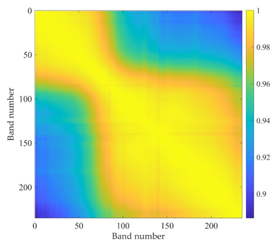
Figure 2.
Correlation coefficients between the 235 bands.
The correlation coefficients between 8 bands selected according to equal band number spacing and some images of these bands are presented in Appendix C.
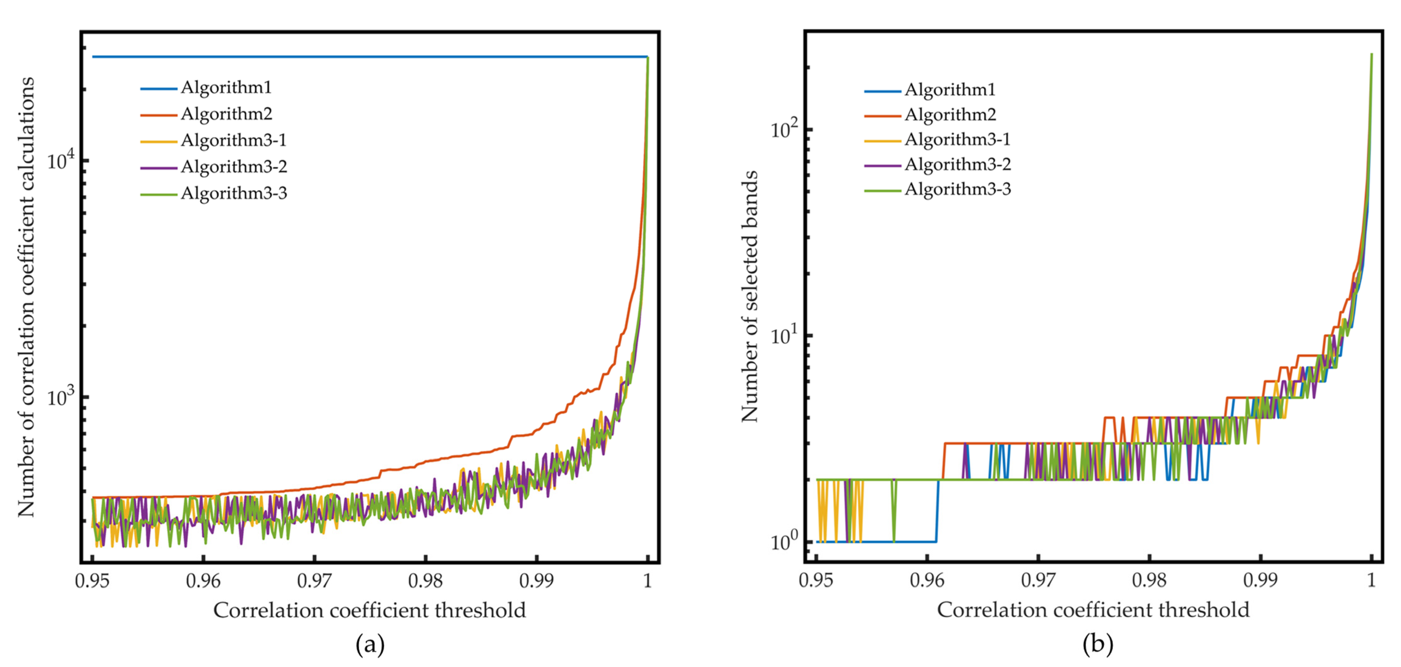
The number of correlation coefficient calculations and the number of selected bands of the three algorithms under different correlation coefficient thresholds are presented in Figure 3. Since the result of Algorithm 3 has certain randomness, the results of the three times are given in the figure. It can be seen that before the correlation coefficient threshold reaches 0.995, the num of selected bands is always less than 10, which again reveals the high redundancy between bands.
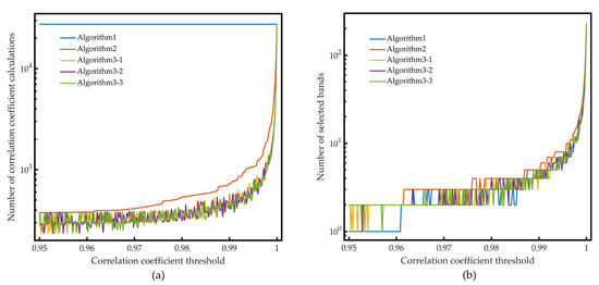
Figure 3.
Comparison of the three compression algorithms based on data selection: (a) The number of correlation coefficient calculations. (b) The number of selected bands of the three algorithms under different correlation coefficient thresholds.
The specific values when the correlation coefficient thresholds are 0.997, 0.998, 0.999, and 0.9996 are presented in Table 2 and Table 3.
Table 2.
The number of correlation coefficient calculations of the three algorithms under four selected correlation coefficient thresholds.
Table 3.
The number of the selected bands of the three algorithms under four selected correlation coefficient thresholds.
It can be seen from Table 2 and Table 3 and Figure 3 that Algorithm 3 has the best operational efficiency, and the number of correlation coefficient calculations of Algorithm 3 under the four selected thresholds is about half of Algorithm 2. When the correlation coefficient threshold is set to 0.997, the correlation calculation times of Algorithm 3 is only about 3% of Algorithm 1, and for most of the thresholds, this ratio is less than 10%. Regarding the number of selected bands after compression, Algorithm 1 performs best because it has the complete correlation information of all the bands. The number of the bands selected by Algorithm 3 is only about 10% more than Algorithm 1, while the amount of calculation is significantly reduced. Besides, the number of the bands selected by Algorithm 3 is about 20% less than Algorithm 2.
In spectral compression, there are only 235 bands, and even the number of correlation coefficient calculations of Algorithm 1 is acceptable. Therefore, Algorithm 1 is selected for the spectral compression. According to the results of Algorithm 1, 40 and 8 bands are selected to generate the datasets S40 and S8 when the correlation coefficient threshold is set to 0.997 and 0.9996.
4.1.2. Compression Algorithm Based on PCA
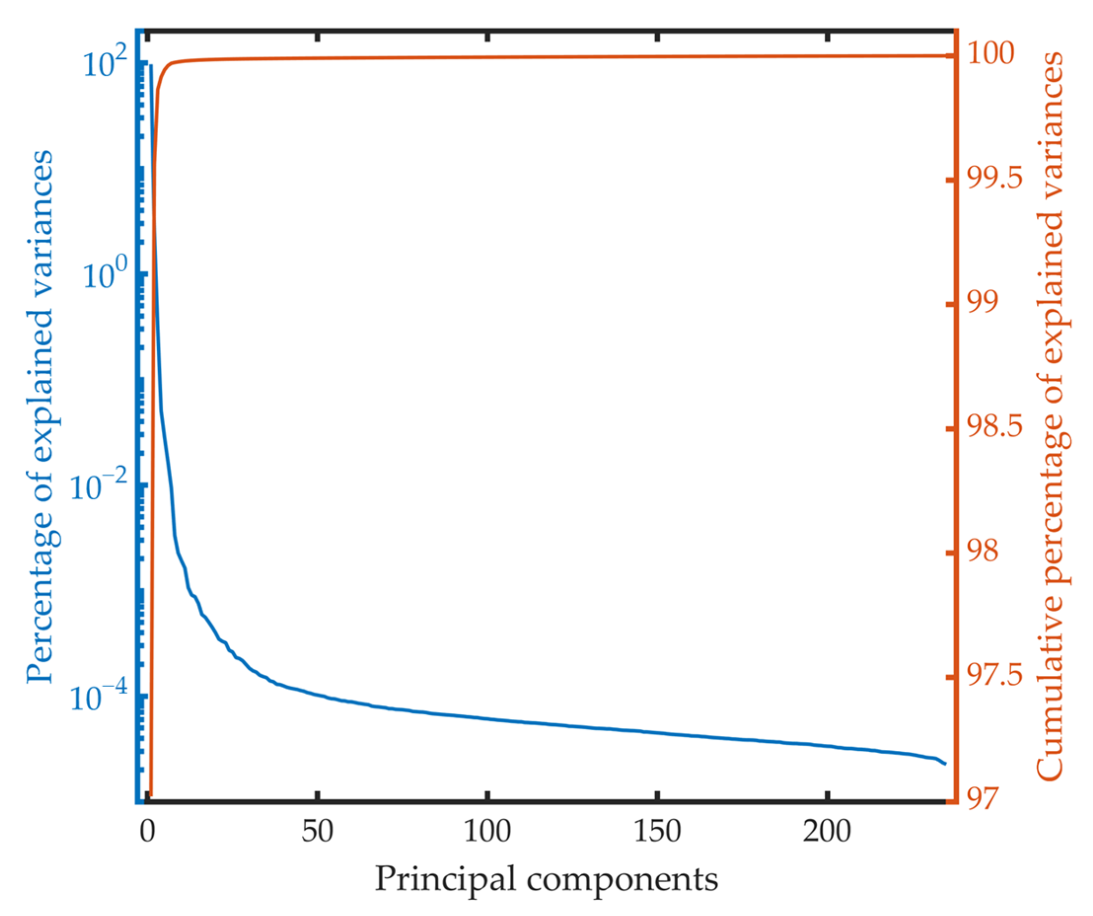
When the compression algorithm based on PCA is applied in the training dataset, the percentage of explained variances of each principal component and the cumulative percentage of explained variances are presented in Figure 4. As can be observed from this figure, the percentage of explained variances decreases rapidly with the increase of the principal component number. The percentage of explained variances of the first principal component reaches 97.0211%. The sum of the first two principal components is 99.5647%, which indicates the high redundancy in the spectral dimension again. The percentage of explained variances decreases gradually after the 10th principal component and forms a long tail.

Figure 4.
The percentage of explained variances of each principal component and the cumulative percentage of the explained variances.
To compare with the algorithm based on data selection, the number of the principal components is also set to 40 and 8, respectively, and two datasets named P40 and P8 are generated. The cumulative percentage of explained variances of the first 40 and the first 8 principal components is 99.9895% and 99.9735%, respectively.
4.2. Comparision of Models Trained on Different Compressed Datasets
In order to find the influence of different spectral compression algorithms on model training speed and the performance of the trained model, the following datasets are constructed.
- 235: the original dataset with 235 bands;
- S40: dataset with 40 bands constructed by using compression algorithm based on data selection;
- P40: dataset with 40 principal components constructed by using compression algorithm based on PCA;
- S8: dataset with eight bands constructed by using compression algorithm based on data selection;
- P8: dataset with 8 principal components constructed by using compression algorithm based on PCA;
- S40P8: dataset with eight principal components constructed by using compression algorithm based on PCA on dataset S40;
For the branch network, if bands are grouped in band number order, adjacent bands with high correlation will be assigned to the same branch. Therefore, the data fed to branch networks might be more diverse by disrupting the original band order, and it might be beneficial for the model training. To minimize the correlation between bands in the same group, the 235 bands were randomly reordered 10,000 times, and the sum of the correlation coefficients in each group was calculated. At last, the reordered band number with the minimum correlation coefficients sum is selected to construct a new dataset.
- R235: dataset with 235 bands constructed by reordering the bands of dataset 235;
- SR40: dataset with 40 bands constructed by reordering the bands of dataset S40.
Under the same hardware configuration, the batch size of the model training is set as large as possible. The hardware configuration of the computer is CPU (Intel i5-10400F, Intel, Santa Clara, CA, USA), memory (16 GB × 2, DDR4 2133 MHz), GPU (Nvidia GeForce RTX3070Ti, 8 GB, Micro-Star, Nvidia, Santa Clara, CA, USA), SSD (Samsung 870 EVO 500 GB, Samsung, Seoul, Korea), HDD (Seagate ST4000DM004, 4TB, Seagate Technology, Fremont, CA, USA). When the number of the selected bands or the principal components (hereinafter referred to as spectral features) is 235, the batch size is set to 16. When the number of the spectral features is 40 and 8, the batch size is set to 32 and 64, respectively.
The SR models were trained based on the datasets mentioned above. The training time for 20 epochs and the SR reconstruction time of one 128 (height) × 128 (width) data are presented in Table 4. This table shows that when compared with the model trained on datasets with 235 spectral features, and when the number of the spectral features is compressed to 40 and 8, the training time is reduced to 30% and 21%, and the SR reconstruction time is reduced to 23% and 6%.
Table 4.
Comparison of training time (20 epochs) and SR reconstruction time.
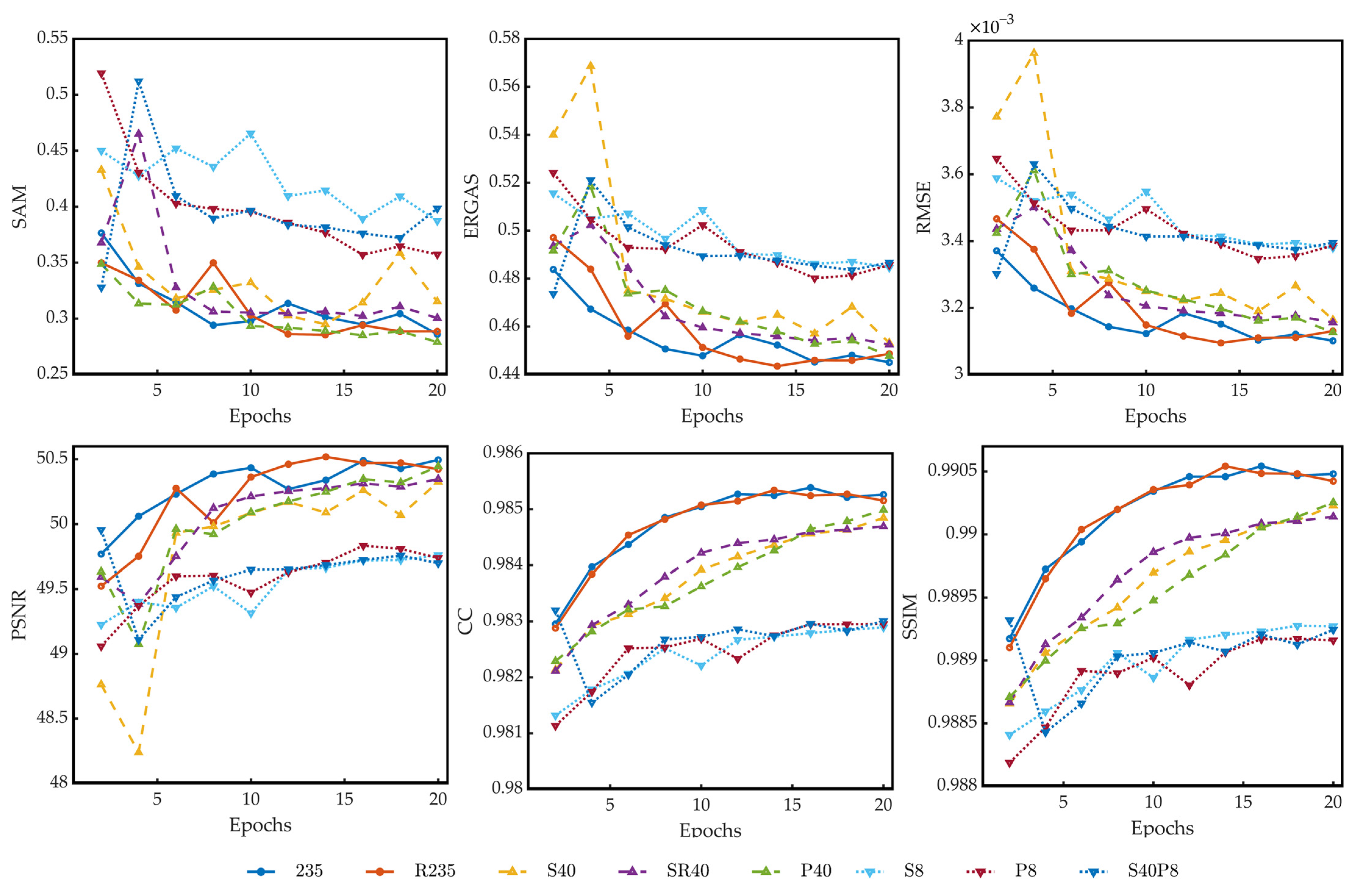
Spectral angle mapper (SAM) [45], erreur relative globale adimensionnelle de synthèse (ERGAS) [46], root mean squared error (RMSE), peak signal-to-noise ratio (PSNR), cross-correlation (CC) [47], and structure similarity (SSIM) [48] are used to evaluate the performance of models trained on different datasets. The PSNR and SSIM of the reconstructed hyperspectral images are the mean values of all spectral bands. The best values for these indices are 0, 0, 0, +∞, 1, and 1, respectively [37].
Figure 5 presents the performance data obtained by SR reconstructing the test dataset on models trained on different datasets under different epochs. Unsurprisingly, models trained on datasets with 235 bands perform best because there is no information loss in these datasets. Besides, for datasets with 235 bands, band reordering has nearly no effect on model improvement. That might be because the dataset contains too much redundant information, which would be repeatedly learned by the model. Therefore, even though the data fed to the branch network are highly correlated, the model can still be well trained. The model trained on dataset 235 is set as the benchmark.
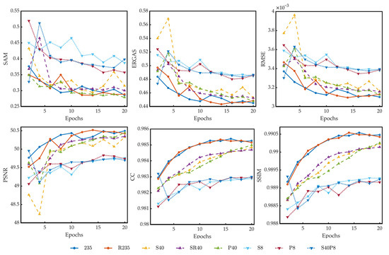
Figure 5.
The performance of models trained on different datasets under different epochs. SAM(Spectral Angle Mapper), ERGAS(Erreur Relative Globale Adimensionnelle de Synthèse), RMSE(Root Mean Squared Error), PSNR(Peak Signal-To-Noise Ratio), CC(Cross-Correlation), and SSIM(Structural Similarity Index Measure are used for the performance evaluation.
It can be seen from Figure 5 that when the number of the spectral features is compressed to 40, the trained models still perform very well both in terms of spectral characteristics and spatial characteristics. The model trained on dataset SR40 performs better and more stably than the model trained on dataset S40. When the number of the spectral features is further compressed to 8, there is a clear gap between the performance of these trained models and the benchmark, no matter how the dataset is compressed, and the performances of these three models are nearly the same.
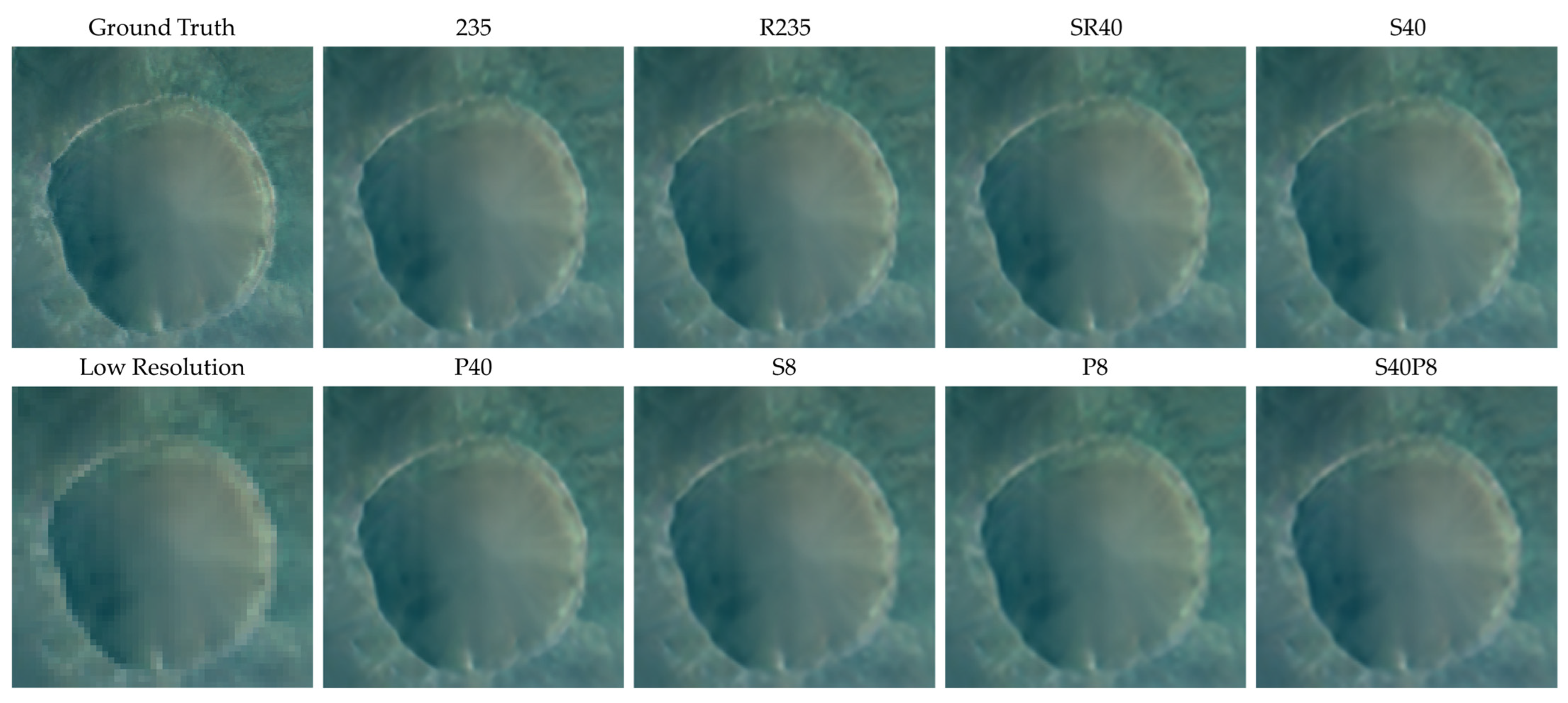
Part of the SR reconstruction images of test data frt000050f2_07_if165l_trr3 using models trained on different datasets under the same training epochs (twenty epochs) is presented in Figure 6. In this figure, the spatial resolution of the ground truth and the SR reconstruction images is 200 × 200, and the spatial resolution of the low-resolution image is 50 × 50. Three bands with central wavelengths of 2.53 μm, 1.51 μm, and 1.1 μm are selected as R, G, and B channels to synthesize these pseudo-color images. All the pixels were linearly stretched by the same scale factor to make the difference between these images more visible. It can be seen from the figure that when the number of spectral features is 235 or 40, the images are almost the same, and there is no discernible difference. When the number of spectral features reduces to 8, the crater edge becomes more blurred and wider. In addition, the ground truth data is selected as the benchmark in Figure 7. The reason is to evaluate the RMSE of all 235 bands between the benchmark and the other images. It can be observed more clearly that when the number of spectral features is 235 or 40, the difference between the SR reconstructed images is small. When the number of spectral features reduces to 8, the difference between the right edge and the crater interior is more apparent.
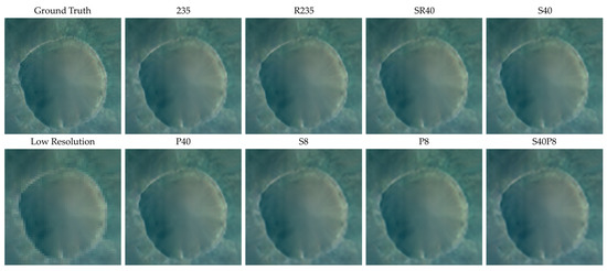
Figure 6.
Comparison of the ground truth and the SR reconstruction images. The images in the first column are the original high-resolution (ground truth) and low-resolution images. The images in the other four columns are the SR reconstruction images reconstructed by the models trained on different datasets, and the name of the datasets are labeled in the titles of these images.
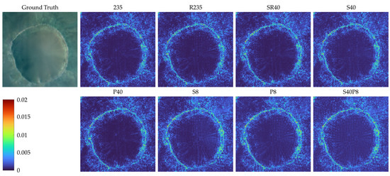
Figure 7.
The RMSE of all 235 bands between the ground truth and the SR reconstruction images. The image in the first column are the original high-resolution (ground truth) image. The images in the other four columns are the RMSE of all 235 bands between the ground truth and the SR reconstruction data reconstructed by the models trained on different datasets, and the name of the datasets are labeled in the titles of these images.
4.3. Spatial Compression
In spatial compression, the correlation coefficients between low-resolution patches are calculated first, and the results of datasets 235, S40, and P40 are presented in Figure 8. It can be observed from the figure that there are noticeable differences among them. The reason is that when the correlation coefficients between patches are calculated directly, the correlations of spatial and spectral dimensions are mixed. In the principal component analysis in the spectral dimension, it can be found that the percentages of explained variances of the leading principal components are very high. Therefore, the percentages of explained variances of the following principal components are rather low, which means that the value range of these principal components is rather limited and eventually leads to the high correlation coefficient between patches.
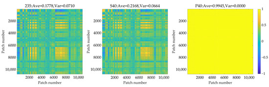
Figure 8.
The correlation coefficients between patches of datasets 235, S40, and P40.
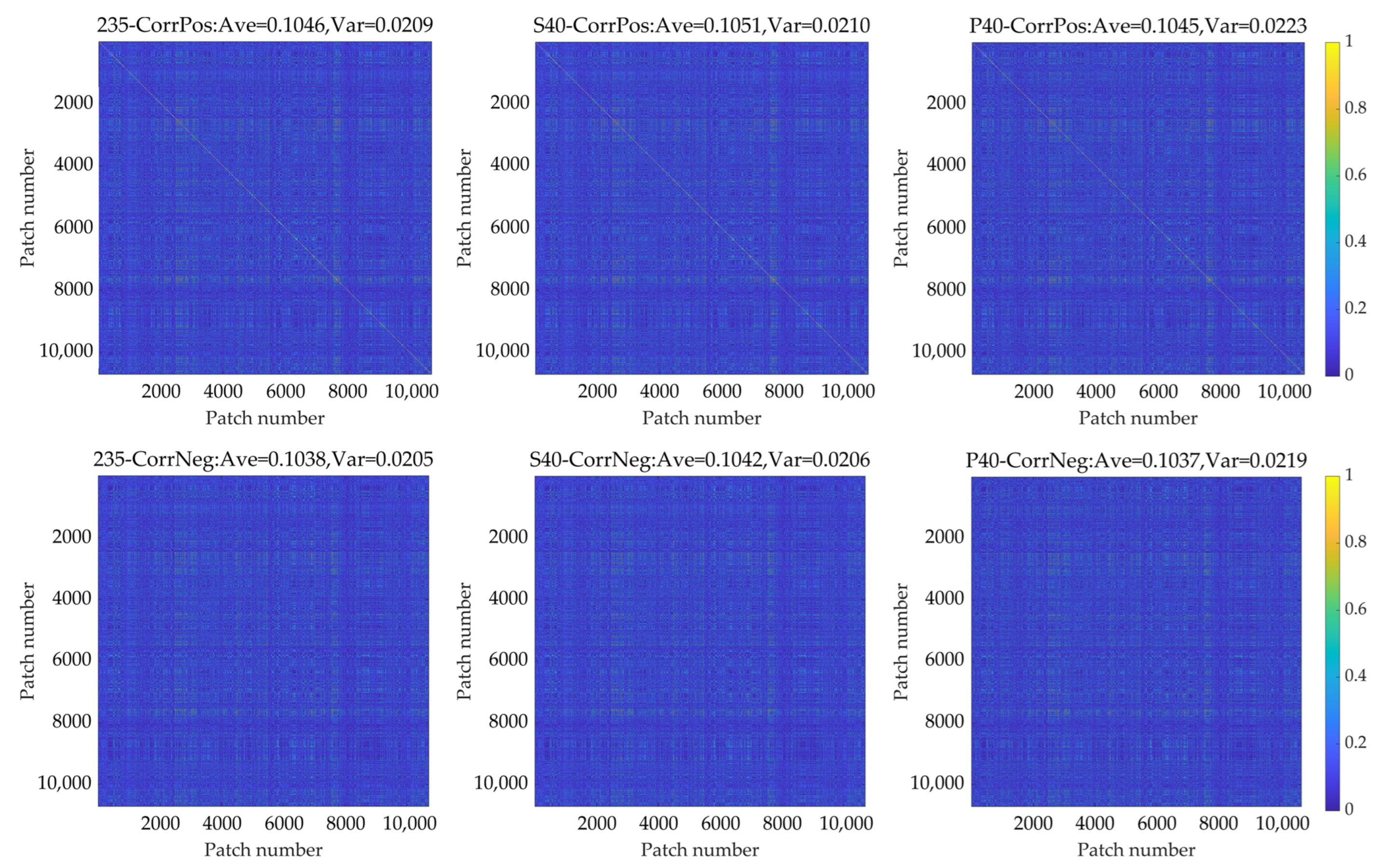
To exclude the influence of the spectral dimension and get the correlation coefficients between patches in the spatial dimension, the correlation coefficients between patches can be calculated according to Equations (2)–(5). The correlation coefficients between patches of datasets 235, S40, and P40 calculated in this way are presented in Figure 9.
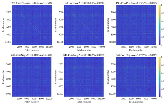
Figure 9.
The correlation coefficients between patches of dataset 235, S40, and P40 were calculated according to Equations (2) and (3).
The results of these three datasets are very close to each other. It indicates that the calculation method proposed in this paper is unaffected by spectral compression. In spectral compression, the band correlation coefficient threshold of S40 is set to 0.9996, and the cumulative percentage of explained variances of the first 40 principal components reaches 99.9895%. Thus, the information of the patches is preserved very well, and the performance of the models trained on datasets 235, S40, and P40 is nearly the same. So, it is reasonable for the correlation coefficients between patches to be close in datasets 235, S40, and P40. The spatial correlation between patches is mainly derived from the similarity of the Martian surface texture features in these patches. It can be seen from the figure that the spatial correlation between patches is relatively low, which shows the diversity of spatial texture. The analysis of the relationship between the calculated correlation coefficients and the spatial texture of patches and the histogram of the CorrPhase of dataset 235 are presented in Appendix D. The results indicate that the CorrPos and CorrNeg can reflect the correlation of spatial texture between patches accurately. The signs of the correlation coefficients between patches are highly consistent in each spectral feature.
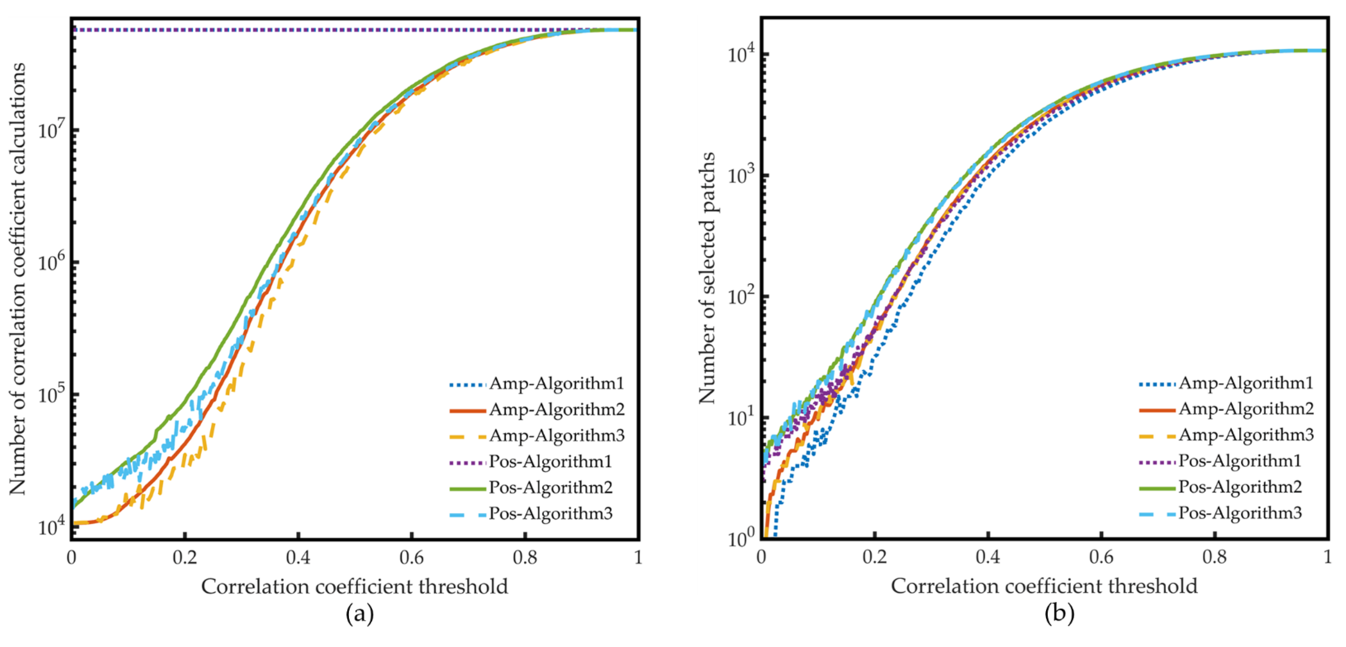
Because moderate spectral compression could reduce the model training time and the SR reconstruction runtime significantly with almost no accuracy loss, the spatial compression is performed on the dataset SR40. It can be found from Equations (2)–(5) that the correlation coefficients between patches have nothing to do with the band order; thus, the patch correlation coefficients of the dataset SR40 are just the same as the dataset S40. The same three algorithms used in spectral compression are also used in spatial compression, and the results are plotted in Figure 10. Since the result calculated by Algorithm 3 has randomness, the data of Algorithm 3 in the figure is the average of three runs.
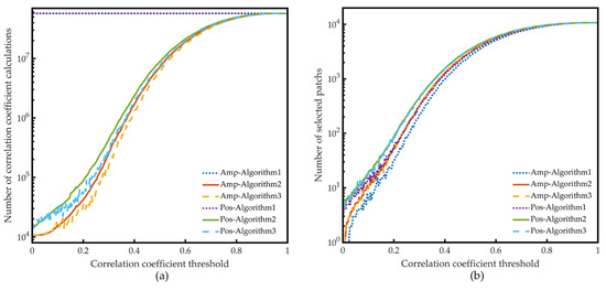
Figure 10.
Comparison of the three compression algorithms based on data selection: (a) the number of correlation coefficient calculations and (b) the number of selected patches of the three algorithms under different correlation coefficient thresholds. (Amp means the correlation coefficient thresholds are set for CorrAmp, and Pos means the correlation coefficient thresholds are set for CorrPos.).
As can be observed in Figure 10, although in spatial compression, Algorithm 3 still performed better than Algorithm 2, the improvement is limited. The reason is that although patches with adjacent numbers might be close to each other in the spatial dimension and even have certain overlapping regions, these effects on the spatial correlation between patches are not decisive, and the scope of these effects is limited. Therefore, the correlation between the patch number and the patch correlation coefficients is inherently random, and Algorithms 2 and 3 are nearly equivalent. Similar to the spectral compression, when the correlation coefficient threshold is relatively low compared with the correlation coefficients of patches, many patches with high correlation coefficients are removed quickly in Algorithms 2 and 3. It significantly reduces the number of correlation coefficient calculations compared with Algorithm 1. To find the effect of spatial compression on model training speed and the performance of the trained model, the spatial compression ratios are set to 12.5%, 25%, 50%, and 75%. Since the negative correlation means a different trend of texture change, CorrPos was selected as the correlation criterion for patch selection. Because of the compression efficiency and the uniqueness of the operation result, Algorithm 2 is selected for spatial compression. Finally, the CorrPos thresholds set for algorithm 2 are 0.385, 0.458, 0.576, and 0.692, and the number of the selected patches are 1349, 2688, 5372, and 8037, which are 12.59%, 25.09%, 50.14%, and 75.02% of the total number of patches in the training dataset.
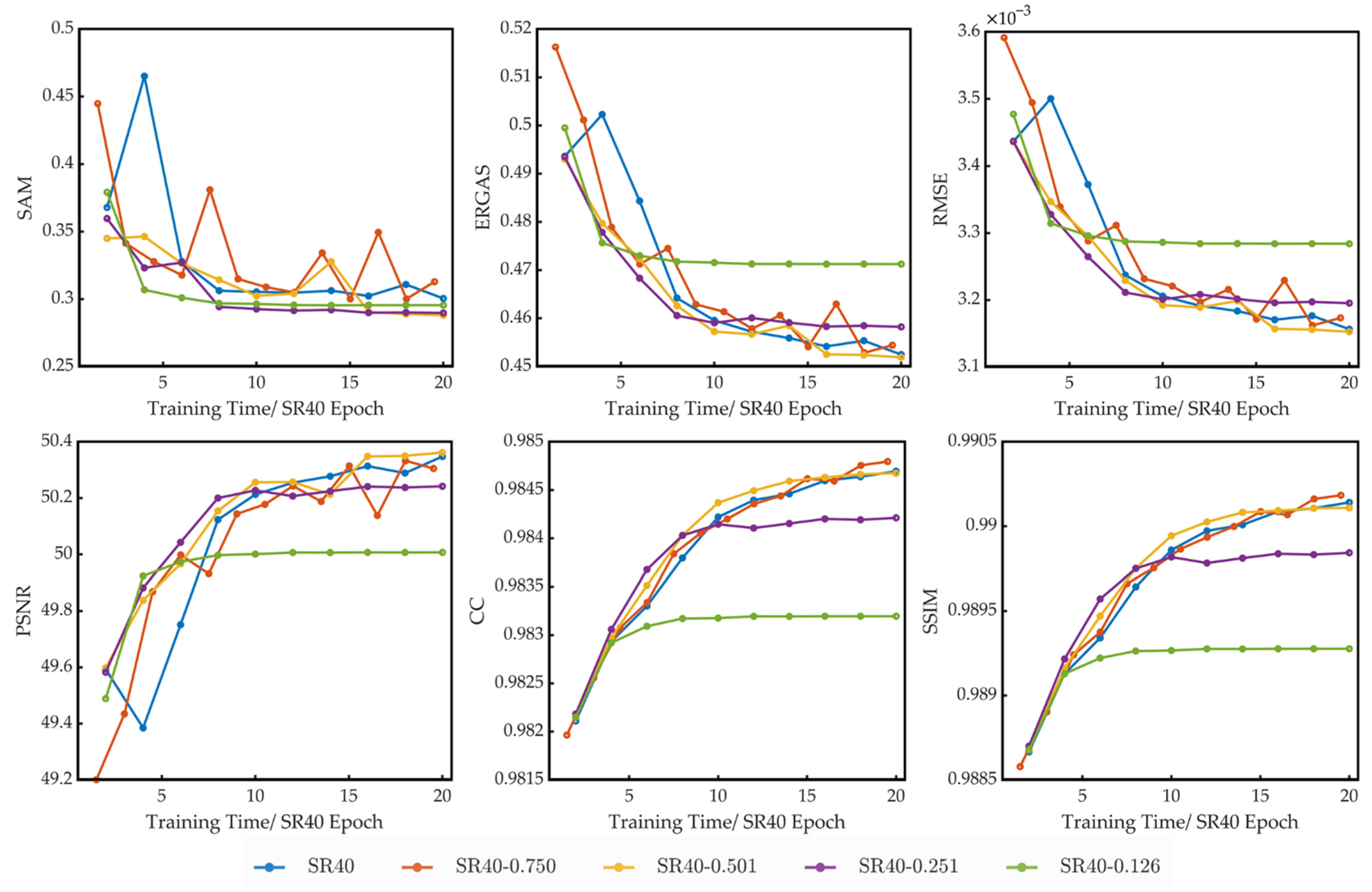
The performance of models trained on different spatial compression datasets under different training times is presented in Figure 11. In this figure, the horizontal axis is the training time in units of the SR40 epoch, which is about 14 min for each SR40 epoch. For spatial compression datasets, the training time of each epoch and the number of patches in training datasets are reduced in the same proportion.
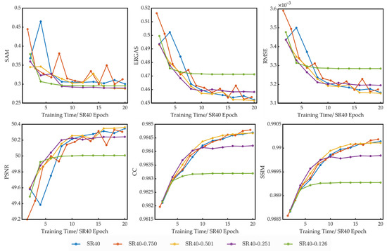
Figure 11.
The performance of models trained on different spatial compression datasets with different training times.
It can be seen from these figures that when the spatial compression ratio is higher than 0.5, the training speed of the models and the performance of the models are nearly the same. When the ratio is lower than 0.25, the quantitative picture quality indices (except for the SAM) start to worsen with the compression ratio reduction. So, due to the low spatial correlation between patches, the spatial compression cannot improve the training speed or the performance of the trained model. However, it proves the redundancy of the dataset in the spatial dimension. The model can be well trained with only half of the original patches.
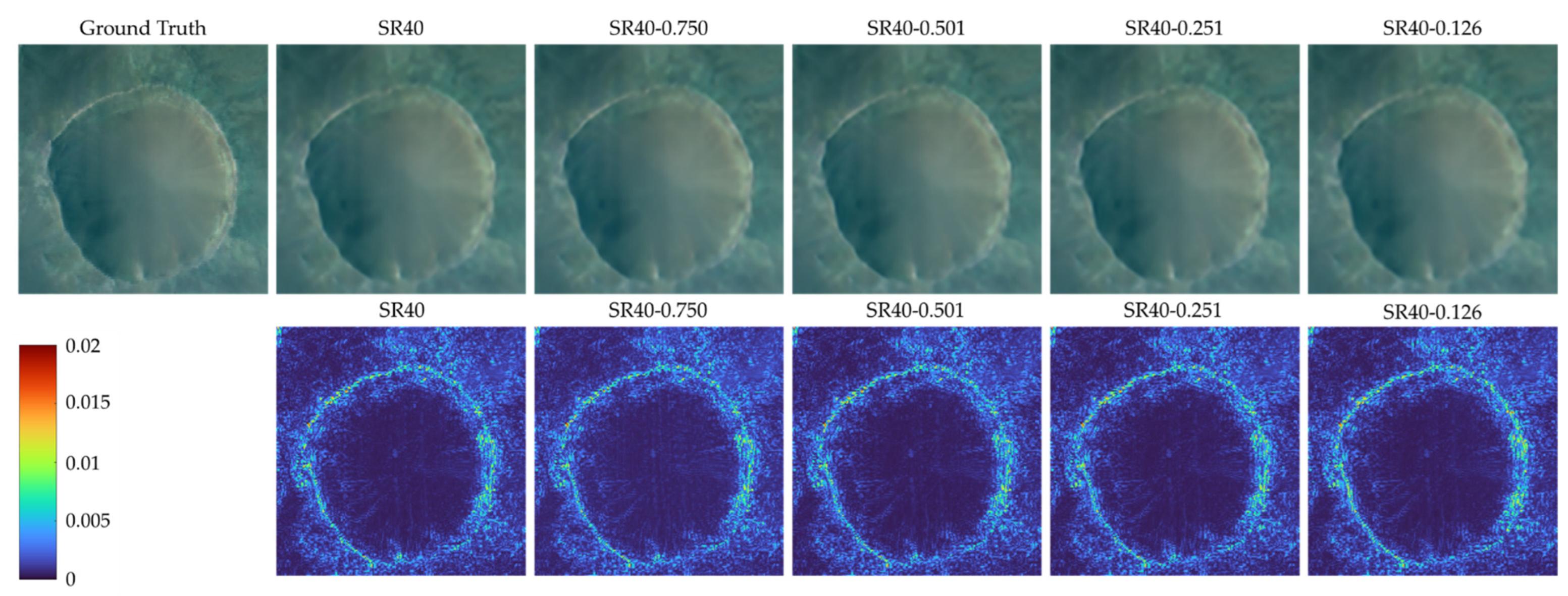
The SR reconstruction images of test data frt000050f2_07_if165l_trr3 using models trained on different datasets with nearly the same training time (19.5 SR40 epochs for SR40-0.750 and 20 SR40 epochs for the other datasets) are presented in Figure 12. In addition, the RMSE result of all 235 bands between the ground truth and the SR reconstruction images based on the models trained on these datasets are also presented in Figure 12. The differences between these SR reconstruction images are subtle. It can be observed from Figure 5 and Figure 11 that the performance gap of the models trained with different spatial compression datasets is smaller than the performance gap of the models trained with different spectral compression datasets. That is why the differences between the images in Figure 12 are more subtle than in Figure 6.

Figure 12.
Comparison of the ground truth and the SR reconstruction images and the RMSE of all 235 bands between the ground truth and the other SR reconstruction images.
5. Discussion
This paper proposes a network model that can perform SR in both spectral and spatial dimensions, and a CRISM dataset is created for model training first. Then the compression algorithms in both spectral and spatial dimensions are being researched to optimize the model training and the SR construction speed.
5.1. Spectral Compression
Three algorithms based on data selection and one algorithm based on PCA are applied to the CRISM dataset for data compression in spectral dimension. The results of spectral compression can be summarized as follows.
The original dataset is highly correlated in the spectral dimension. Moderate spectral compression can significantly reduce the model training time and the SR reconstruction runtime with nearly no loss of accuracy. Compared with the performance of the original dataset with 235 bands, when the number of the spectral features is compressed to 40, training time and SR reconstruction runtime can be reduced to 30% and 23%. After the spectral compression, the correlation between bands in each branch group can be reduced by reordering these bands. It can make each branch network obtain more diverse information in the model training so that the model can be trained better.
The performance of the compression algorithms based on data selection and PCA is nearly the same. When the number of principal components is only one or two, or even eight, although the proportion of explained variances of the leading principal components is high, the information contained in these principal components can not ensure the model can be trained well. To enrich the spectral information of the compressed dataset, more principal components need to be included. Since the explained variances proportions of the following principal components are pretty low, the number of the principal components needs to be increased significantly. Therefore, the compression algorithm based on PCA has no prominent advantage in compression rate compared with the compression algorithms based on data selection. Besides, in compression algorithms based on data selection, spectral compression can be completed by directly extracting selected bands from the original data with almost no computation. All the selected bands have clear physical meaning. While in compression algorithm based on PCA, the principal components needed to be obtained by matrix multiplications and have no explicit physical meaning. Therefore, the compression algorithm based on data selection is more suitable for the spectral compression of the original dataset and performs well.
5.2. Spatial Compression
A new method for spatial correlation evaluation of hyperspectral data is proposed in spatial compression. The proposed evaluating indicators CorrPos and CorrNeg can reflect the correlation of spatial texture between patches well. The correlation of patches in spatial dimensions between patches is relatively low.
The training time and the performances of the models trained on the datasets with different spatial compression ratios indicate that the spatial compression has nearly no effect when the ratio is higher than 0.5. When the spatial compression ratio reduces to 0.25, the performance of the trained models becomes worse and worse with the reduction of the compression ratio, even if the training time is long enough. This means that the dataset with half patches has contained sufficient mapping information between the low-resolution and high-resolution data. Therefore, the model can be trained well with the same training time. But when the compression ratio is lower than 0.25, the mapping information contained in the dataset becomes incomplete. Therefore, even if the time of the model training is long enough, there will still be a gap between the performance of the model trained on the compressed dataset and the model trained on the complete dataset. When the compression ratio decreases further, the performance degradation of the trained model will aggravate further.
Therefore, the amount of data in the dataset is not just ‘the more, the better’. When the dataset contains enough mapping information, the newly added data is useless for the model training. It can be used to check the completeness of the dataset by correlation analysis.
6. Conclusions
In this paper, to apply the SR algorithm based on deep learning to hyperspectral remote sensing data more effectively, the correlation of the CRISM dataset in both spectral and spatial dimensions is analyzed in detail. A network that can perform spatial SR and spectral enhancement simultaneously and some data compression algorithms based on data selection or PCA are proposed.
The results indicate that when the number of the bands is compressed to 40, training time and SR reconstruction runtime can be reduced to 30% and 23% with almost no accuracy loss. The effectiveness of compression algorithms based on data selection indicates that maybe not all the bands need to be transmitted from the Mars probes or be collected. It would, in principle, help improve the efficiency of satellite data transmission and simplify the design of the hyper-spectrometer. Because the trained model can perform spectral enhancement, the algorithm and the network may also be used for the abnormal band and invalid data recovery. In addition, the datasets used for model training in this paper are created based on the Targeted Reduced Data Record (TRDR) of CRISM. To realize the complete mapping model between the spectral compressed raw data received from the Mars probes and the final spatial SR reconstructed and spectrally enhanced outputs, the radiometric calibration algorithm based on the spectral compressed raw data needs to and will be developed and integrated into the proposed model in the future work. The validity of the complete mapping model will also be fully tested on more kinds of hyperspectral remote sensing data to verify the feasibility of onboard spectral compression.
In spatial compression, it can be observed that the model could be trained well with only half of the original data. It indicates that the completeness of the dataset can be checked by analyzing the correlations between the data.
Author Contributions
Conceptualization, M.S. and S.C.; methodology, M.S.; software, M.S.; validation, M.S. and S.C.; formal analysis, M.S.; investigation, M.S.; resources, M.S. and S.C.; data curation, M.S.; writing—original draft preparation, M.S.; writing—review and editing, M.S.; visualization, M.S.; supervision, S.C.; project administration, S.C.; funding acquisition, S.C. All authors have read and agreed to the published version of the manuscript.
Funding
This work is supported by the National Key Research and Development Program of China (Grant No. 2020YFE0202100) and the National Key Research and Development Program of China (No. 2020YFA0714103).
Data Availability Statement
CRISM original data are available at http://pds-geosciences.wustl.edu/missions/mro/crism.htm and were accessed on 20 February 2021.
Acknowledgments
We would like to thank the Mars Reconnaissance Orbiter team for building the spacecraft and the CRISM team for providing the CRISM dataset. We thank the PDS Geosciences Node website for providing the CRISM data used in this study.
Conflicts of Interest
The authors declare no conflict of interest.
Appendix A
Table A1.
Product IDs of the selected CRISM data.
Table A1.
Product IDs of the selected CRISM data.
| Index | Product ID | Index | Product ID | Index | Product ID |
|---|---|---|---|---|---|
| 1 | frt0000a8ce_07_if166l_trr3 | 20 | frt000165f7_07_if166l_trr3 | 39 | frt000093be_07_if166l_trr3 |
| 2 | frt0000a09c_07_if166l_trr3 | 21 | frt0000634b_07_if163l_trr3 | 40 | frt000095fe_07_if166l_trr3 |
| 3 | frt0000a33c_07_if164l_trr3 | 22 | frt0001756e_07_if164l_trr3 | 41 | frt000097e2_07_if166l_trr3 |
| 4 | frt0000a063_07_if165l_trr3 | 23 | frt00008144_07_if164l_trr3 | 42 | frt000135db_07_if166l_trr3 |
| 5 | frt0000a425_07_if166l_trr3 | 24 | frt00009824_07_if164l_trr3 | 43 | frt000174f4_07_if166l_trr3 |
| 6 | frt0000a546_07_if165l_trr3 | 25 | frt00003bfb_07_if166l_trr3 | 44 | frt000199c7_07_if166l_trr3 |
| 7 | frt0000aa03_07_if166l_trr3 | 26 | frt00003e12_07_if166l_trr3 | 45 | frt000251c0_07_if165l_trr3 |
| 8 | frt0000abcb_07_if166l_trr3 | 27 | frt00003fb9_07_if166l_trr3 | 46 | frt0000406b_07_if165l_trr3 |
| 9 | frt0000ada4_07_if168l_trr3 | 28 | frt00005a3e_07_if165l_trr3 | 47 | frt0000979c_07_if165l_trr3 |
| 10 | frt0000bda8_07_if165l_trr3 | 29 | frt00009d31_07_if164l_trr3 | 48 | frt0001642e_07_if166l_trr3 |
| 11 | frt0000a106_07_if163l_trr3 | 30 | frt00013d3b_07_if165l_trr3 | 49 | frt0001821c_07_if166l_trr3 |
| 12 | frt0000a377_07_if165l_trr3 | 31 | frt00016a73_07_if166l_trr3 | 50 | frt00003584_07_if166l_trr3 |
| 13 | frt0001b615_07_if166l_trr3 | 32 | frt00018dca_07_if166l_trr3 | 51 | frt00009971_07_if166l_trr3 |
| 14 | frt00004af7_07_if164l_trr3 | 33 | frt00019daa_07_if165l_trr3 | 52 | frt00017103_07_if165l_trr3 |
| 15 | frt00008c90_07_if163l_trr3 | 34 | frt00024c1a_07_if165l_trr3 | 53 | frt00018781_07_if165l_trr3 |
| 16 | frt000028ba_07_if165l_trr3 | 35 | frt000047a3_07_if166l_trr3 | 54 | frt00019538_07_if166l_trr3 |
| 17 | frt000035db_07_if164l_trr3 | 36 | frt000048b2_07_if165l_trr3 | 55 | frt00023565_07_if166l_trr3 |
| 18 | frt000128d0_07_if165l_trr3 | 37 | frt000050f2_07_if165l_trr3 | 56 | frt00023728_07_if166l_trr3 |
| 19 | frt000161ef_07_if167l_trr3 | 38 | frt000064d9_07_if166l_trr3 | 57 | frt000088d0_07_if166l_trr3 |
Appendix B
In the SSPSR network, the input low-resolution hyperspectral image is first divided into several overlap groups. For each group, a branch network is applied to extract the spatial-spectral features of the input grouped hyperspectral images (a subset of the entire hyperspectral linages) and upscale them with a smaller upsampling factor (compared with the final target). And then, the output features of all branches are concatenated and fed to the following global spatial-spectral feature extraction and upsampling networks. To let the spatial-spectral prior network (SSPN) in the branch network and global network share the same structure, a “reconstruction” layer was inserted after each branch upsampling module. A global residual structure is also adapted to facilitate the prediction of the target. And the SSPN is constructed by cascading multiple spatial-spectral blocks (SSBs). For each SSB, it contains a spatial residual module and a spectral attention residual module.
The overall network architecture of the SSPSR network and the network architecture of the spatial-spectral block (SSB) can be found in Figures 1 and 2 of reference [37]. The in Figure 1 of reference [37] is the low-resolution hyperspectral image, is the grouped data fed to each branch network, is a Bicubic upsampling version of the input low-resolution hyperspectral images, and is the output high-resolution hyperspectral image.
The model training parameters are set as follows. The scale factor is set to 4. The number of the spectral bands in each group and the overlap between neighboring groups were set to 8 and 2. And the ADAM optimizer with an initial learning rate of 1 × 10⁻⁴, which decays by a factor of 10 when it reaches 30 epochs, is used to adjust the learning rate. In the SSPN, the number of spatial-spectral blocks is set to 3, and the size of all Conv layers to 3 × 3 except for that in the spectral residual modules, where the kernel size is set to 1 × 1. The zero-padding strategy is applied for these Conv layers with kernel size 3 × 3. The Conv layers in shallow feature extraction and SSPN have 256 filters, except in the channel-downscaling. Data augment, including all possible flipping and rotation (integer multiples of 90 degrees), is used to enhance the richness of the data.
Appendix C
Table A2 shows the correlation coefficients between 8 bands selected according to equal band number spacing.
Table A2.
Correlation coefficients matrix between 8 bands.
Table A2.
Correlation coefficients matrix between 8 bands.
| Band Number | 1 | 34 | 67 | 100 | 133 | 166 | 199 | 232 |
|---|---|---|---|---|---|---|---|---|
| 1 | 1.0000 | 0.9960 | 0.9841 | 0.9413 | 0.9248 | 0.9119 | 0.9061 | 0.8889 |
| 34 | 0.9960 | 1.0000 | 0.9926 | 0.9529 | 0.9373 | 0.9286 | 0.9244 | 0.9107 |
| 67 | 0.9841 | 0.9926 | 1.0000 | 0.9803 | 0.9686 | 0.9623 | 0.9571 | 0.9431 |
| 100 | 0.9413 | 0.9529 | 0.9803 | 1.0000 | 0.9956 | 0.9939 | 0.9863 | 0.9698 |
| 133 | 0.9248 | 0.9373 | 0.9686 | 0.9956 | 1.0000 | 0.9968 | 0.9918 | 0.9780 |
| 166 | 0.9119 | 0.9286 | 0.9623 | 0.9939 | 0.9968 | 1.0000 | 0.9967 | 0.9848 |
| 199 | 0.9061 | 0.9244 | 0.9571 | 0.9863 | 0.9918 | 0.9967 | 1.0000 | 0.9942 |
| 232 | 0.8889 | 0.9107 | 0.9431 | 0.9698 | 0.9780 | 0.9848 | 0.9942 | 1.0000 |
Besides, the low-resolution images of the eight bands of two test data are presented in Figure A1 and Figure A2. Different colors are used instead of grayscales to represent different values to make the difference between different bands more visible. It can also be seen from these two figures that the images of different bands are pretty similar to each other. As the difference of the band number, that is, the difference of the central wavelength of the band, becomes larger, the difference between the corresponding images also becomes more significant.
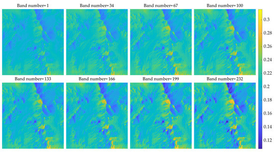
Figure A1.
Comparison of 8 bands of frt00004af7_07_if164l_trr3 low-resolution data.
Figure A1.
Comparison of 8 bands of frt00004af7_07_if164l_trr3 low-resolution data.
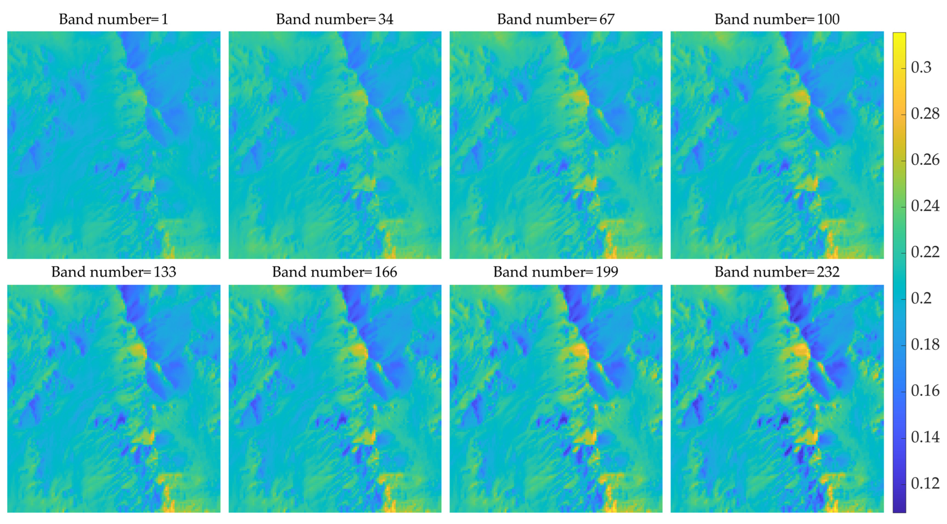
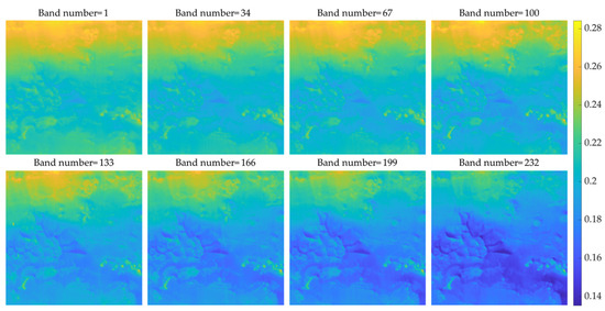
Figure A2.
Comparison of 8 bands of frt000128d0_07_if165l_trr3 low-resolution data.
Figure A2.
Comparison of 8 bands of frt000128d0_07_if165l_trr3 low-resolution data.

Appendix D
To present the relationship between the calculated correlation coefficients and the spatial texture of patches visually, several groups of patches of dataset 235 with high or low correlation coefficients are selected, and the data of the band with a central wavelength of 1.51 μm are drawn in Figure A3. Some of the correlation coefficients between these patches are listed in Table A3. It can be found from this table that patch 1 and patch 2, patch 3, and patch 4 are highly positively correlated, while patch 1 and patch 2 are highly negatively correlated with patch 3 and patch 4. There is no correlation between patch 5 and patch 6, patch 7 and patch 8, while there is a specific negative correlation between patch 5 and patch 8. These conclusions are consistent with the spatial texture variation of these patches presented in Figure A3. It indicates that the CorrPos and CorrNeg can reflect the correlation of spatial texture between patches well.
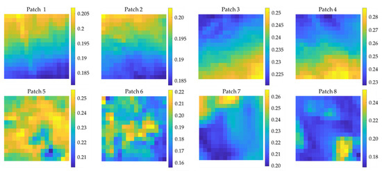
Figure A3.
Spatial textures of patches with high or low correlation coefficients.
Figure A3.
Spatial textures of patches with high or low correlation coefficients.

Table A3.
Part of the correlation coefficients between patches presented in Figure A3.
Table A3.
Part of the correlation coefficients between patches presented in Figure A3.
| CorrPos | Patch 1 | Patch 2 | Patch 3 | Patch 4 | CorrNeg | Patch 1 | Patch 2 | Patch 3 | Patch 4 |
| Patch 1 | 1.00 | 0.95 | 0.00 | 0.00 | Patch 1 | 0.00 | 0.00 | 0.95 | 0.96 |
| Patch 2 | 0.95 | 1.00 | 0.00 | 0.00 | Patch 2 | 0.00 | 0.00 | 0.92 | 0.96 |
| Patch 3 | 0.00 | 0.00 | 1.00 | 0.92 | Patch 3 | 0.95 | 0.92 | 0.00 | 0.00 |
| Patch 4 | 0.00 | 0.00 | 0.92 | 1.00 | Patch 4 | 0.96 | 0.96 | 0.00 | 0.00 |
| CorrPos | Patch 5 | Patch 6 | Patch 7 | Patch 8 | CorrNeg | Patch 5 | Patch 6 | Patch 7 | Patch 8 |
| Patch 5 | 1.00 | 0.00 | 0.00 | 0.00 | Patch 5 | 0.00 | 0.00 | 0.08 | 0.44 |
| Patch 6 | 0.00 | 1.00 | 0.00 | 0.00 | Patch 6 | 0.00 | 0.00 | 0.04 | 0.13 |
| Patch 7 | 0.00 | 0.00 | 1.00 | 0.00 | Patch 7 | 0.08 | 0.04 | 0.00 | 0.00 |
| Patch 8 | 0.00 | 0.00 | 0.00 | 1.00 | Patch 8 | 0.44 | 0.13 | 0.00 | 0.00 |
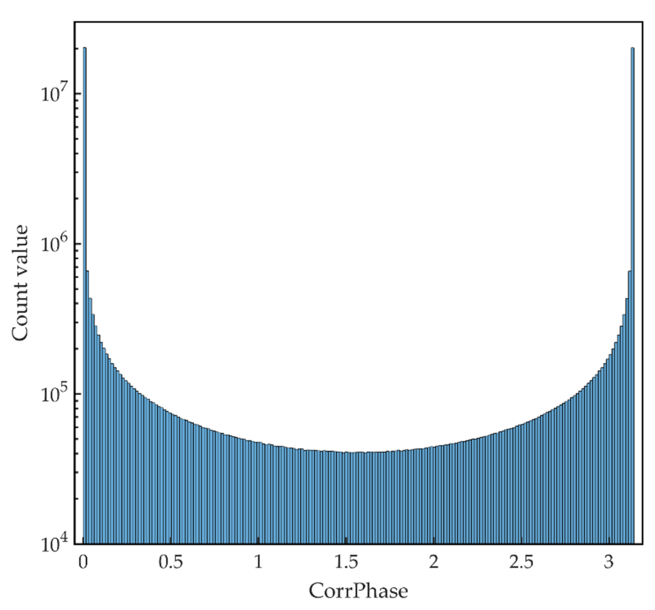
The histogram of the CorrPhase of dataset 235 is presented in Figure A4. In this histogram, the bin size of the histogram is π/200. Only the correlation coefficients between different patches will be counted, and the correlation coefficient of two patches will be counted only once regardless of their order. It can be seen from the histogram that most of the CorrPhase values are concentrated around 0 and π. The signs of the correlation coefficients between patches are highly consistent in each spectral feature.

Figure A4.
The histogram of CorrPhase of dataset 235.
Figure A4.
The histogram of CorrPhase of dataset 235.
References
- Schmidt, R.; Credland, J.D.; Chicarro, A.; Moulinier, P. ESA’s Mars Express mission—Europe on its way to Mars. ESA Bulletin. Bull. ASE. Eur. Space Agency 1999, 98, 56–66. [Google Scholar]
- Chapman, C.R.; Pollack, J.B.; Sagan, C. An analysis of the Mariner 4 photography of Mars; Smithsonian Institution Astrophysical Observatory: Cambridge, MA, USA, 1968. [Google Scholar]
- Howell, E.; Stein, V. Mars Missions: A Brief History. Available online: https://www.space.com/13558-historic-mars-missions.html (accessed on 22 June 2022).
- Ehlmann, B.; Anderson, F.; Andrews-Hanna, J.; Catling, D.; Christensen, P.; Cohen, B.; Dressing, C.; Edwards, C.; Elkins-Tanton, L.; Farley, K. The sustainability of habitability on terrestrial planets: Insights, questions, and needed measurements from Mars for understanding the evolution of Earth-like worlds. J. Geophys. Res. Planets 2016, 121, 1927–1961. [Google Scholar] [CrossRef]
- Farmer, J. Thermophiles, early biosphere evolution, and the origin of life on Earth: Implications for the exobiological exploration of Mars. J. Geophys. Res. Planets 1998, 103, 28457–28461. [Google Scholar] [CrossRef]
- Grotzinger, J.; Beaty, D.; Dromart, G.; Gupta, S.; Harris, M.; Hurowitz, J.; Kocurek, G.; McLennan, S.; Milliken, R.; Ori, G.G. Mars Sedimentary Geology: Key Concepts and Outstanding Questions; Mary Ann Liebert, Inc.: New Rochelle, NY, USA, 2011. [Google Scholar]
- McKay, C.P.; Stoker, C.R. The early environment and its evolution on Mars: Implication for life. Rev. Geophys. 1989, 27, 189–214. [Google Scholar] [CrossRef] [Green Version]
- Poulet, F.; Bibring, J.-P.; Mustard, J.; Gendrin, A.; Mangold, N.; Langevin, Y.; Arvidson, R.; Gondet, B.; Gomez, C. Phyllosilicates on Mars and implications for early Martian climate. Nature 2005, 438, 623–627. [Google Scholar] [CrossRef]
- Read, P.; Lewis, S.; Mulholland, D. The physics of Martian weather and climate: A review. Rep. Prog. Phys. 2015, 78, 125901. [Google Scholar] [CrossRef] [Green Version]
- Christensen, E.J. Martian topography derived from occultation, radar, spectral, and optical measurements. J. Geophys. Res. 1975, 80, 2909–2913. [Google Scholar] [CrossRef]
- Zuber, M.T.; Solomon, S.C.; Phillips, R.J.; Smith, D.E.; Tyler, G.L.; Aharonson, O.; Balmino, G.; Banerdt, W.B.; Head, J.W.; Johnson, C.L. Internal structure and early thermal evolution of Mars from Mars Global Surveyor topography and gravity. Science 2000, 287, 1788–1793. [Google Scholar] [CrossRef] [Green Version]
- Bibring, J.P.; Erard, S. The Martian surface composition. Space Sci. Rev. 2001, 96, 293–316. [Google Scholar] [CrossRef]
- Bandfield, J.L.; Hamilton, V.E.; Christensen, P.R. A global view of Martian surface compositions from MGS-TES. Science 2000, 287, 1626–1630. [Google Scholar] [CrossRef] [Green Version]
- Richardson, M.I.; Mischna, M.A. Long-term evolution of transient liquid water on Mars. J. Geophys. Res. Planets 2005, 110, E03003. [Google Scholar] [CrossRef] [Green Version]
- Clifford, S.M.; Lasue, J.; Heggy, E.; Boisson, J.; McGovern, P.; Max, M.D. Depth of the Martian cryosphere: Revised estimates and implications for the existence and detection of subpermafrost groundwater. J. Geophys. Res. Planets 2010, 115, E07001. [Google Scholar] [CrossRef]
- Rogers, A.D.; Hamilton, V.E. Compositional provinces of Mars from statistical analyses of TES, GRS, OMEGA and CRISM data. J. Geophys. Res. Planets 2015, 120, 62–91. [Google Scholar] [CrossRef]
- Zou, Y.; Zhu, Y.; Bai, Y.; Wang, L.; Jia, Y.; Shen, W.; Fan, Y.; Liu, Y.; Wang, C.; Zhang, A. Scientific objectives and payloads of Tianwen-1, China’s first Mars exploration mission. Adv. Space Res. 2021, 67, 812–823. [Google Scholar] [CrossRef]
- Nawar, S.; Buddenbaum, H.; Hill, J.; Kozak, J. Modeling and mapping of soil salinity with reflectance spectroscopy and landsat data using two quantitative methods (PLSR and MARS). Remote Sens. 2014, 6, 10813–10834. [Google Scholar] [CrossRef] [Green Version]
- Thomas, M.; Walter, M.R. Application of hyperspectral infrared analysis of hydrothermal alteration on Earth and Mars. Astrobiology 2002, 2, 335–351. [Google Scholar] [CrossRef] [Green Version]
- Zhang, L.; Du, B.; Zhong, Y. Hybrid detectors based on selective endmembers. IEEE Trans. Geosci. Remote Sens. 2010, 48, 2633–2646. [Google Scholar] [CrossRef]
- Zhou, F.; Yang, W.; Liao, Q. Interpolation-based image super-resolution using multisurface fitting. IEEE Trans. Image Process. 2012, 21, 3312–3318. [Google Scholar] [CrossRef]
- Rajan, D.; Chaudhuri, S. Generalized interpolation and its application in super-resolution imaging. Image Vis. Comput. 2001, 19, 957–969. [Google Scholar] [CrossRef]
- Park, S.C.; Park, M.K.; Kang, M.G. Super-resolution image reconstruction: A technical overview. IEEE Signal Process. Mag. 2003, 20, 21–36. [Google Scholar] [CrossRef] [Green Version]
- Li, J.; Cui, R.; Li, B.; Song, R.; Li, Y.; Du, Q. Hyperspectral Image Super-Resolution with 1D–2D Attentional Convolutional Neural Network. Remote Sens. 2019, 11, 2859. [Google Scholar] [CrossRef] [Green Version]
- Zou, C.; Huang, X. Hyperspectral image super-resolution combining with deep learning and spectral unmixing. Signal Process. Image Commun. 2020, 84, 115833. [Google Scholar] [CrossRef]
- Wang, Q.; Li, Q.; Li, X. Hyperspectral Image Superresolution Using Spectrum and Feature Context. IEEE Trans. Ind. Electron. 2021, 68, 11276–11285. [Google Scholar] [CrossRef]
- Ha, V.K.; Ren, J.; Xu, X.; Zhao, S.; Xie, G.; Vargas, V.M. Deep Learning Based Single Image Super-Resolution: A Survey. In Proceedings of the International Conference on Brain Inspired Cognitive Systems, Xi’an, China, 7–8 July 2018; pp. 106–119. [Google Scholar]
- Ma, W.; Pan, Z.; Yuan, F.; Lei, B. Super-Resolution of Remote Sensing Images via a Dense Residual Generative Adversarial Network. Remote Sens. 2019, 11, 2578. [Google Scholar] [CrossRef] [Green Version]
- Liu, Y.; Liu, S.; Wang, Z. A general framework for image fusion based on multi-scale transform and sparse representation. Inf. Fusion 2015, 24, 147–164. [Google Scholar] [CrossRef]
- Dong, C.; Loy, C.C.; He, K.; Tang, X. Learning a Deep Convolutional Network for Image Super-Resolution. In Proceedings of the European Conference on Computer Vision (ECCV), Zurich, Switzerland, 6–12 September 2014. [Google Scholar]
- He, K.; Zhang, X.; Ren, S.; Sun, J. Deep Residual Learning for Image Recognition. In Proceedings of the IEEE Conference on Computer Vision and Pattern Recognition, Las Vegas, NV, USA, 27–30 June 2016; pp. 770–778. [Google Scholar]
- Kim, J.; Lee, J.K.; Lee, K.M. Accurate Image Super-Resolution Using Very Deep Convolutional Networks. In Proceedings of the IEEE Conference on Computer Vision and Pattern Recognition, Las Vegas, NV, USA, 27–30 June 2016; pp. 1646–1654. [Google Scholar]
- Hu, J.; Li, Y.; Xie, W. Hyperspectral Image Super-Resolution by Spectral Difference Learning and Spatial Error Correction. IEEE Geosci. Remote Sens. Lett. 2017, 14, 1825–1829. [Google Scholar] [CrossRef]
- Zheng, K.; Gao, L.; Zhang, B.; Cui, X. Multi-Losses Function Based Convolution Neural Network for Single Hyperspectral Image SuperResolutio. In Proceedings of the 2018 Fifth International Workshop on Earth Observation and Remote Sensing Applications (EORSA), Xi’an, China, 18–20 June 2018; pp. 1–4. [Google Scholar]
- Li, Y.; Zhang, L.; Ding, C.; Wei, W.; Zhang, Y. Single Hyperspectral Image Super-resolution with Grouped Deep Recursive Residual Network. In Proceedings of the 2018 IEEE Fourth International Conference on Multimedia Big Data (BigMM), Xi’an, China, 13–16 September 2018; pp. 1–4. [Google Scholar]
- Liu, W.; Lee, J. An Efficient Residual Learning Neural Network for Hyperspectral Image Super resolution. IEEE J. Sel. Top. Appl. Earth Obs. Remote Sens. 2019, 12, 1240–1253. [Google Scholar] [CrossRef]
- Jiang, J.; Sun, H.; Liu, X.; Ma, J. Learning spatial-spectral prior for super-resolution of hyperspectral imagery. IEEE Trans. Comput. Imaging 2020, 6, 1082–1096. [Google Scholar] [CrossRef]
- Murchie, S. Compact Reconnaissance Imaging Spectrometer for Mars (CRISM) on Mars Reconnaissance Orbiter (MRO). J. Geophys. Res. Atmos. 2007, 112, E05S03. [Google Scholar] [CrossRef]
- Morgan, M.; Seelos, F.; Murchie, S. The CRISM Analysis Toolkit (CAT): Overview and Recent Updates. In Proceedings of the Third Planetary Data Workshop and the Planetary Geologic Mappers Annual Meeting, Flagstaff, Arizona, 12–15 June 2017; p. 7121. [Google Scholar]
- Amador, E.S.; Bandfield, J.L.; Thomas, N.H. A search for minerals associated with serpentinization across Mars using CRISM spectral data. Icarus 2018, 311, 113–134. [Google Scholar] [CrossRef]
- Tian, L.; Fan, C.; Ming, Y.; Jin, Y. Stacked PCA network (SPCANet): An Effective Deep Learning for Face Recognition. In Proceedings of the 2015 IEEE International Conference on Digital Signal Processing (DSP), Singapore, 21–24 July 2015; pp. 1039–1043. [Google Scholar]
- Valpola, H. From Neural PCA to Deep Unsupervised Learning. In Advances in Independent Component Analysis and Learning Machines; Elsevier: Amsterdam, The Netherlands, 2015; pp. 143–171. [Google Scholar]
- Chen, Y.; Lin, Z.; Zhao, X.; Wang, G.; Gu, Y. Deep learning-based classification of hyperspectral data. IEEE J. Sel. Top. Appl. Earth Obs. Remote Sens. 2014, 7, 2094–2107. [Google Scholar] [CrossRef]
- Jolliffe, I. Pincipal Component Analysis; Springer: Berlin/Heidelberg, Germany, 2002; Volume 25, p. 513. [Google Scholar]
- Yuhas, R.H.; Goetz, A.F.; Boardman, J.W. Discrimination Among Semi-Arid Landscape Endmembers Using the Spectral Angle Mapper (SAM) Algorithm. In Proceedings of the JPL, Summaries of the Third Annual JPL Airborne Geoscience Workshop, Volume 1: AVIRIS Workshop, Pasadena, CA, USA, 1–5 June 1992; pp. 147–149. [Google Scholar]
- Wald, L. Data Fusion: Definitions and Architectures: Fusion of Images of Different Spatial Resolutions; Presses des MINES: Paris, France, 2002. [Google Scholar]
- Loncan, L.; De Almeida, L.B.; Bioucas-Dias, J.M.; Briottet, X.; Chanussot, J.; Dobigeon, N.; Fabre, S.; Liao, W.; Licciardi, G.A.; Simoes, M. Hyperspectral pansharpening: A review. IEEE Geosci. Remote Sens. Mag. 2015, 3, 27–46. [Google Scholar] [CrossRef] [Green Version]
- Wang, Z.; Bovik, A.C.; Sheikh, H.R.; Simoncelli, E.P. Image quality assessment: From error visibility to structural similarity. IEEE Trans. Image Process. 2004, 13, 600–612. [Google Scholar] [CrossRef] [PubMed] [Green Version]


Publisher’s Note: MDPI stays neutral with regard to jurisdictional claims in published maps and institutional affiliations. |
© 2022 by the authors. Licensee MDPI, Basel, Switzerland. This article is an open access article distributed under the terms and conditions of the Creative Commons Attribution (CC BY) license (https://creativecommons.org/licenses/by/4.0/).