Article

Estimation of Maize Yield and Flowering Time Using Multi-Temporal UAV-Based Hyperspectral Data

1
Biological Systems Engineering, University of Wisconsin–Madison, Madison, WI 53706, USA
2
Department of Agronomy, University of Wisconsin–Madison, Madison, WI 53706, USA
*
Author to whom correspondence should be addressed.
Remote Sens. 2022, 14(13), 3052; https://doi.org/10.3390/rs14133052
Submission received: 29 April 2022 / Revised: 13 June 2022 / Accepted: 23 June 2022 / Published: 25 June 2022

Abstract

:
Maize (Zea mays L.) is one of the most consumed grains in the world. Within the context of continuous climate change and the reduced availability of arable land, it is urgent to breed new maize varieties and screen for the desired traits, e.g., high yield and strong stress tolerance. Traditional phenotyping methods relying on manual assessment are time-consuming and prone to human errors. Recently, the application of uncrewed aerial vehicles (UAVs) has gained increasing attention in plant phenotyping due to their efficiency in data collection. Moreover, hyperspectral sensors integrated with UAVs can offer data streams with high spectral and spatial resolutions, which are valuable for estimating plant traits. In this study, we collected UAV hyperspectral imagery over a maize breeding field biweekly across the growing season, resulting in 11 data collections in total. Multiple machine learning models were developed to estimate the grain yield and flowering time of the maize breeding lines using the hyperspectral imagery. The performance of the machine learning models and the efficacy of different hyperspectral features were evaluated. The results showed that the models with the multi-temporal imagery outperformed those with imagery from single data collections, and the ridge regression using the full band reflectance achieved the best estimation accuracies, with the correlation coefficients (r) between the estimates and ground truth of 0.54 for grain yield, 0.91 for days to silking, and 0.92 for days to anthesis. In addition, we assessed the estimation performance with data acquired at different growth stages to identify the good periods for the UAV survey. The best estimation results were achieved using the data collected around the tasseling stage (VT) for the grain yield estimation and around the reproductive stages (R1 or R4) for the flowering time estimation. Our results showed that the robust phenotyping framework proposed in this study has great potential to help breeders efficiently estimate key agronomic traits at early growth stages.

1. Introduction

The world is facing crop production challenges due to the rapid expansion of the human population and the adverse agricultural environments caused by climate change, urbanization, soil degradation, water shortages, and pollution [1,2,3,4]. Breeding new varieties of major crops to achieve higher yield potential and stress tolerance is considered to be a promising solution to ensure food security [5,6,7,8]. Maize (Zea mays L.) is one of the most consumed grains globally, serving as an essential resource for human food, animal feed, and bioenergy [9]. In 2020, the U.S. produced more than 360 million tons of maize, accounting for 34.28% of the total production worldwide [10]. Maize production, nevertheless, is reduced by a few frequently occurring limitations, such as limited water availability or nitrogen deficiency [11,12]. Thus, developing maize varieties with improved yield and environmental adaptability is a primary breeding target [13,14,15]. Advances in high-throughput genotyping have enabled the development of large mapping populations and diversity panels of thousands of recombinant inbred lines for breeding selection [16,17,18]. High-throughput phenotyping has substantial potential to accelerate the selection process and improve the efficiency within the breeding cycle [19]. Conventional phenotyping methods primarily rely on manual assessments and visual ratings [20,21], requiring intense workloads and being prone to human bias [22,23,24]. Therefore, there is an urgent need to develop an advanced high-throughput phenotyping (HTP) framework for breeding maize and other species.
The efficiency of breeding strategies is assessed by genetic gain, i.e., the improvement of the primary trait (grain yield for maize) due to selection within a population over cycles of breeding [25,26]. Timely and accurate estimation of grain yield prior to harvesting is vital for the maize breeding process since it allows breeders to boost the genetic gain by increasing the population size, reducing the phenotypic variability, enhancing the genetic dissection, improving the selection accuracy, and consequently shortening the breeding cycle [23,26,27,28]. Traditionally, breeders evaluate the yield at the end of the season by harvesting maize and measuring the weight of the grain. Even though the harvest is performed with combines, human effort and time are required to evaluate thousands of hybrid lines, making field trials an expensive component of the breeding process. Moreover, breeders often need extensive in-season measurements to fully understand the physiological mechanisms underlying the hybrids with diverse genetic backgrounds and their interactions with the environment. This in-season measurement data will help breeders conduct genome-wide association analyses and dissect the genetic basis of seedling growth, crop stress tolerance, and, finally, improve crop yield [29]. However, measuring plant traits manually in field conditions throughout the growing season is labor-intensive and time-consuming [23,30].
Flowering time is critical in deploying varieties across environments, impacting yield and seed quality in maize [31]. Flowering time reflects the adaptation of a plant to its environment by tailoring vegetative and reproductive phases to local climatic effects [32] and is therefore related to its developmental characteristics such as plant height, total number of leaves, and grain fill [33]. Abiotic stresses, such as drought, will influence maize flowering pathways [34] and extend the anthesis-silking interval [35], leading to adverse effects on the fertilization rate, kernel filling, seed quality, and weight [11,31]. Therefore, monitoring flowering time is critical in selecting superior genotypes for particular target environments in maize breeding programs. Flowering time is typically scored as the date when 50% of the plants in a plot are shedding pollen (Days to Anthesis, DTA) and when 50% of the ears have visible extruded silks (Days to Silking, DTS) [36]. The measurement of flowering time requires regular visual evaluation of each plot during the flowering period, which is time-consuming and requires specialized domain knowledge.
In the past decade, uncrewed aerial vehicles (UAVs) have become a new research frontier in the area of HTP and have been applied to various missions for breeding purposes such as yield estimation [27,36,37] and stress detection [38,39,40]. UAV-based platforms allow an ideal balance between image quality and efficiency for breeding trials with flexible spatial and temporal image resolution selections. Additionally, they are low-cost, user-friendly (in terms of operations and data access), and are more robust to weather conditions when gathering high-quality images. Moreover, UAV platforms have the potential to carry various sensors onboard, supporting an array of modalities.
Research using UAV-based spectral imagery to estimate maize yield and flowering time spans both precision agriculture and breeding applications. In precision agriculture applications, the same maize variety is often sown throughout with different treatments, and VIs are widely used to model the maize yield under these varied conditions. For example, in estimating maize yield under different combinations of fertilizers, Guo et al. (2020) adopted a modified red blue vegetation index derived from UAV-based RGB images, reaching a coefficient of determination (R2) of 0.57 [41]. Peng et al. (2021) integrated UAV multispectral VIs into a simple algorithm for yield (SAFY) crop model, and the estimation reached an agreement of R2 = 0.86 with the ground measured maize yield under different water treatments [42]. Quemada et al. (2014) reported an accuracy of 0.82 (Pearson coefficient r) using two hyperspectral VIs as the predictors of a linear-plateau model in estimating maize yield under different fertilizer rates [43]. Trait estimation for maize hybrids in a breeding program is more challenging than precision agriculture application due to the genotypic complexity of varieties and the limited replicates of hybrids. Wu et al. (2019) estimated the yield of 25 maize hybrids using a VI based on the normalized difference between the blue and near-infrared (NIR) wavelength bands (BNDVI). A partial least squares regression (PLSR) model trained with the time-series BNDVI achieved an average accuracy of r = 0.51 for grain yield and r = 0.69–0.70 for the flowering time [36]. Danilevicz et al. (2021) used multispectral VIs, genotype information, and field management data to predict maize yield of G2F breeding trails, hitting an accuracy of R2 = 0.73 [44]. Herrmann et al. (2020) assessed maize yield over 19 maize hybrids using VIs extracted from a super-spectral sensor mounted on a UAV, reaching an R2 of 0.73 for grain yield prediction [45]. Though successful, most existing studies only used VIs or some suitable bands as features for estimating maize yield and flowering time, at the risk of missing critical spectral details. Moreover, the spectral features used in previous studies were derived from limited growth stages within the growing season, without comprehensive investigations of the effectiveness of spectral features across multiple growth stages.
Motivated by the need to facilitate the phenotyping efficiency in maize breeding, this study aimed to develop a robust HTP framework to estimate the yield and flowering time of large maize breeding populations using UAV-based hyperspectral images. To accomplish this, we: (1) investigated the performances of three widely used machine learning models for maize yield and flowering time estimation, (2) evaluated the effectiveness of four types of spectral features extracted from the hyperspectral images, and (3) identified the best time for the UAV survey. The framework proposed in this study will help maize breeders reduce the resource inputs of selecting the highest-performing varieties by delivering timely and accurate estimates of the traits of interest.

2. Materials and Methods

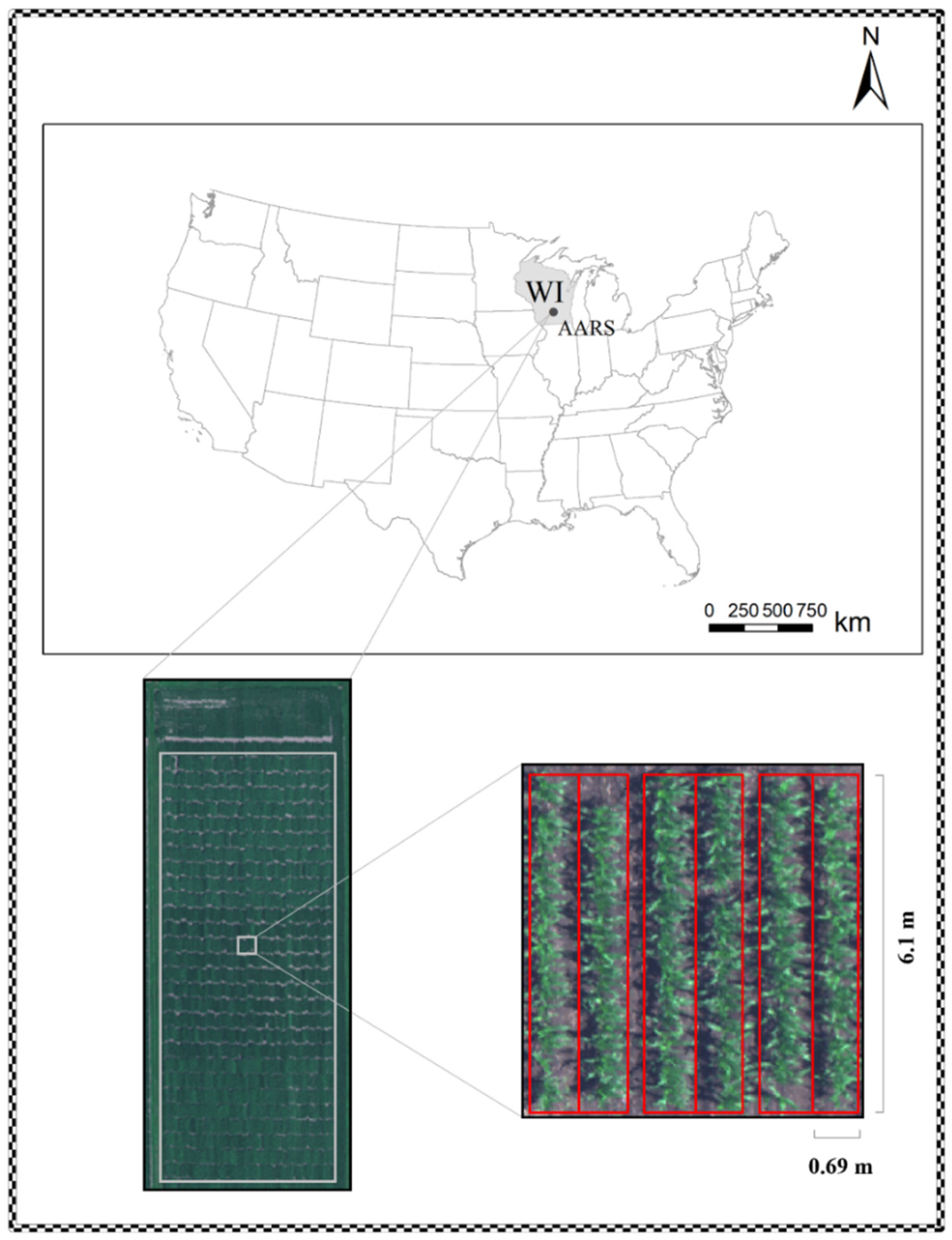
2.1. Field Trials and Ground Truth Data Collection

The field experiment was carried out at the Arlington Agricultural Research Station (AARS) in Wisconsin (latitude: 43°17′40″N, longitude: 89°23′10″W, Figure 1) as a part of the Genomes to Fields (G2F) initiative. G2F is a collaborative research program linking genomics and predictive phenomics for a comprehensive study of genotype-by-environment (GxE) interactions (https://www.genomes2fields.org, (accessed on 10 January 2022)). The AARS was one of the experimental sites in 2020 and experienced warm and humid summers and cold and dry winters. Over 1000 maize hybrids were cultivated under a randomized complete block design. The hybrids were developed from the W10004 population and three inbred testers, namely PHP02, PHK76, and PHZ51. In addition, three check populations were repetitively planted as phenotypic references, including the local checks, external checks, and yellow stripe. They were planted on 13 May 2020, as two-row plots with 6.10 m in length and 0.69 m in row spacing and were harvested on 28 October 2020.
In this study, phenotypic data, including flowering time and grain yield, were collected manually and used for machine learning model development and validation. From early July, flowering time measurement was made by visual inspections on each plot every other day. Specifically, the flowering time for each plot was recorded as the number of days after seeding (DAS) for 50% of the plants in a plot releasing pollen (DTA) and for 50% of the plants in a plot with visibly emerged silks (DTS). The maize plots were harvested at the end of the growing season (late October), and the grain mass and moisture content were measured for each plot. The average crop density was 61 plants per plot at harvest time. Finally, the grain yield was normalized to 15.5% grain moisture.

2.2. Hyperspectral Image Acquisition and Processing

Hyperspectral data were acquired by a Headwall nano-hyperspec push-broom scanner (Headwall Photonics, Inc., Bolton, MA, USA). The scanner featured 274 spectral bands ranging from 400–1000 nm with a bandwidth of 2.2 nm. The DJI Matrice 600 Pro (DJI Technology Co., Shenzhen, China) with a three-axis gimbal stabilizer was utilized as a UAV platform to carry this scanner. In addition, a lightweight navigation system was incorporated with the UAV platform for data geo-referencing. The flight missions were conducted at 42 m above ground at a speed of 5 m/s, having a 2.45 cm ground sampling distance (GSD).
In this study, we conducted 11 UAV surveys between June and October in 2020 under clear and calm weather conditions, covering critical maize vegetative and reproductive stages. The survey dates, corresponding DAS, and growth stages are shown in Table 1.
Two main pre-processing steps were performed after the data acquisition, including geometric correction and radiometric correction. First, we orthorectified hyperspectral data by GNSS/INS data using SpectralView software (Headwall Photonics, Inc., Bolton, MA, USA) for geometric correction. For radiometric correction, the raw digital numbers (DN) of the hyperspectral data were converted into radiance, and then the reflectance was radiometrically calibrated using reference panels with the reflectance of 56%, 32%, and 11%. Image background (e.g., shadow and soil) was removed by setting a threshold at an NIR band because the vegetation often has higher reflectance in the NIR region than the background [46]. Specifically, the pixels with reflectance below 30% at an 800 nm wavelength were removed. Individual plots were separated by manually drawing boundaries outside each plot, and then the average reflectance at different bands was extracted by averaging the reflectance value of all the valid pixels for each plot.

2.3. Spectral Feature Extraction

Four types of commonly used spectral features were extracted from the hyperspectral imagery, including the full band spectral reflectance, vegetation indices (VIs), the first derivatives (FDR), and second derivatives (SDR) of the spectral reflectance.
Full Band Spectral Reflectance: Spectral reflectance indicates light absorption at specific wavelengths and is linked to plant characteristics [47,48,49,50]. The average reflectance values were extracted from the hyperspectral imagery for each plot.
Vegetation Indices: VIs have been widely used in different agricultural applications, as they reflect chemically interpretable absorption in the spectra [51,52,53,54]. In this study, 81 published narrow-band VIs were extracted from the hyperspectral data. Detailed calculations for each VI were summarized in [55].
Derivative Features: The spectral derivatives are relatively insensitive to changes in light intensity caused by sun angle, cloud cover, and terrain [56,57]. Several studies have used derivative features for land-cover classification [58,59,60], plant stress identification [61], and canopy cover estimation [62]. In this study, noises along the full band spectral profile were removed using the Savitzky–Golay filter [63] for each plot. The first derivatives (FDR) and second derivatives (SDR) were then calculated for all the bands along with the smoothed spectra.

2.4. Model Development and Performance Evaluation

To evaluate the differences in spectral profiles between high-yield and low-yield genotypes, a paired sample t-test was performed on the spectral profiles of the top 10% and bottom 10% yield groups. The top 10% group had 121 genotypes with a mean yield of 16.16 ton/ha, while the bottom group had 121 genotypes with a mean yield of 6.24 ton/ha. The paired sample t-test was conducted using the Python SciPy package.
This study trained three widely used machine learning models to estimate the maize grain yield and flowering time using the multi-temporal hyperspectral features. Ridge regression is a widely used model that is superior in analyzing data that suffer from multicollinearity [64,65]. Ridge regression is more robust than linear regression, which has constraints on regression coefficients and thus is less prone to overfitting. Different alpha values, which stand for the regularization strength in ridge regression models, were tested and optimized using the grid search method in this study. Support vector regression (SVR) has good model generalization ability and is widely used [66,67,68]. In SVR, a crucial step is to use a kernel function to map the input variables from the original dimensional space to the high-dimensional feature space. We used the radial basis function (RBF) as the kernel function in this study. These things considered, the hyperparameters of kernel coefficient and the strength of the regularization in the SVR model were grid-searched for the best model performance. Random forest (RF) is an ensemble learning model [69], which is computationally efficient in the training phase and generally has a high generalization accuracy. The RF model consists of a number of individual regression trees, and each tree represents a set of conditions or restrictions [70]. The final predictive results of RF are obtained by averaging the outputs of all individual trees. In this study, the number of trees and the tree depths in the RF model were tested using a grid search to achieve a fair comparison with other models.
The spectral features collected at all 11 times were used as combined inputs to the machine learning models to compare their overall performance in estimating maize yield and flowering time. It led to a dataset including 1429 samples, with each having 3014 features when using the full band original reflectance and the derivatives and 891 features when using the VIs. To evaluate the best UAV survey timing over the growing season, spectral features collected each day were considered as inputs to the machine learning models, leading to 274 features when using the full band original reflectance and the derivatives and to 81 features when using the VIs. The Pearson coefficient ( r ), mean absolute error (MAE), and root mean square error (RMSE) metrics between the estimated values and ground truth data were used as metrics for evaluating the model performance. The models were evaluated using a four-fold cross-validation method, with a random split in each fold of 75% of the data as the training dataset and 25% as the test dataset. The four-fold cross-validation was repeated 20 times to test the model robustness, resulting in 80 experiments of each model and each feature. The testing accuracies were calculated by averaging the estimation results of the 80 experiments.

3. Results and Discussion

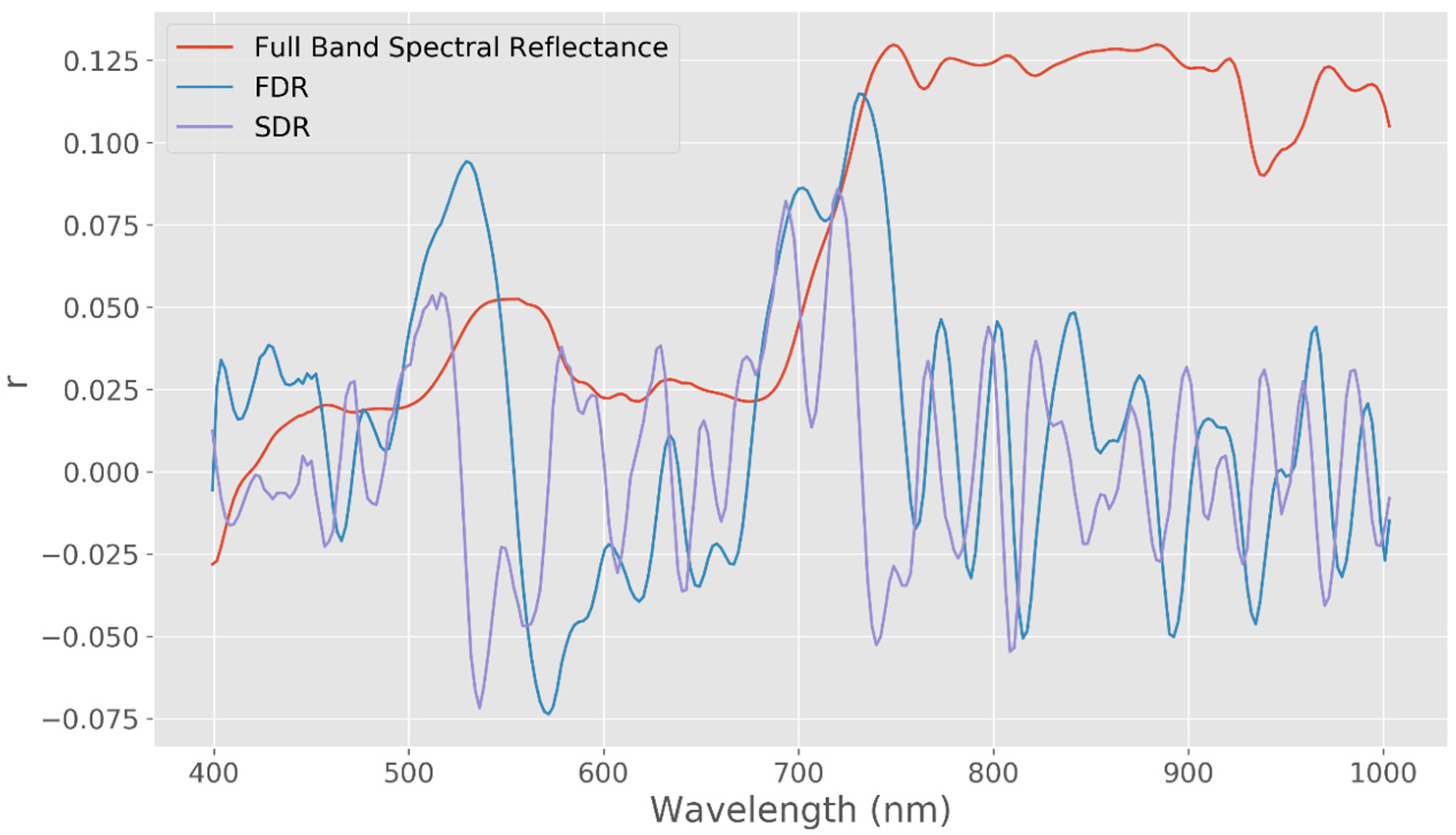
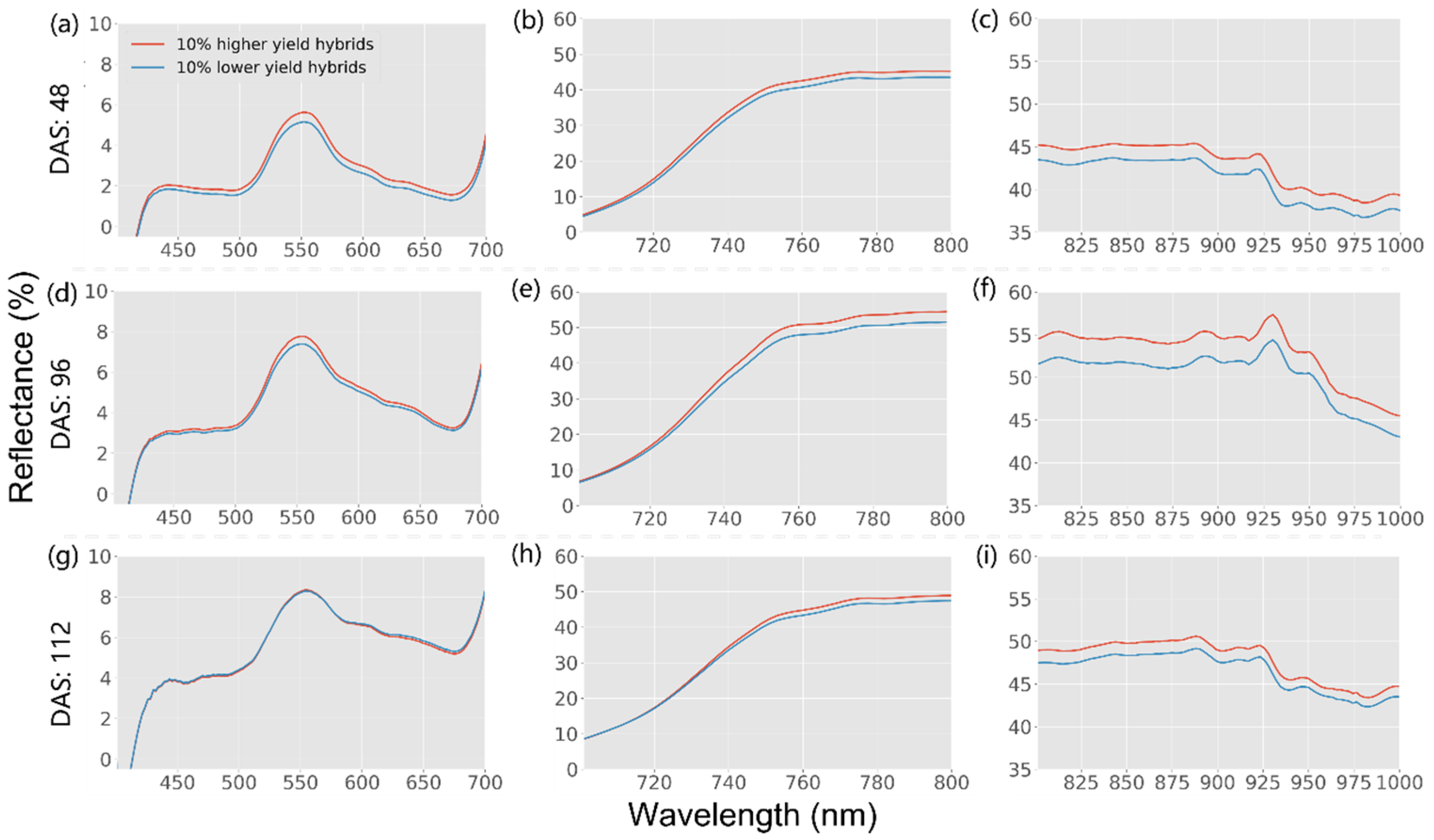
3.1. Ground Truth Field Data and Spectral Profiles

The distributions of grain yield, DTS, and DTA are shown in Figure 2. The average yield over all the plots was 11.5 tons/ha, and the average DTS and DTA were 69 and 67 DAS in this experiment. Figure 3 shows the spectral profiles of the hybrids with the top 10% and bottom 10% yield groups collected at the early (48 DAS), middle (96 DAS), and late growth stages (112 DAS). The paired sample t-test results of the spectral profiles between the two groups are listed in Table 2. From the early to the late growth stages, no significant differences were observed in the 400–700 nm (Figure 3a,d,g) and 700–800 nm regions (Figure 3b,e,h) between these two groups. However, the higher-yield plots tended to have significantly higher reflectance values in the NIR region (800–1000 nm, Figure 3c,f,i) throughout the growing season. Similar findings were also reported on other crops, such as wheat [70,71,72,73], alfalfa [55,74], sorghum [75], and soybean [21,50,76]. This is because higher NIR reflectance values indicate more chlorophyll within plants, representing greater vegetation vigor and health status [77,78,79]. However, when maize plants enter the late growth stage, the NIR region reflectance of the plant canopy decreases because of the increase of image pixels representing silks and tassels. Thus, those with earlier flowering times might have lower NIR reflectance values, and the spectral bands during these stages reflect the interactions of the flowering time, yield potential, and other factors [80,81].

3.2. Estimation Performance by Models and Image Features

The performances of the three machine learning models in estimating the maize yield and flowering time are shown in Table 3. Each of the models were trained separately with full band spectra, FDR, SDR, and VIs. The data from all the 11 flights were combined as the model inputs. The highest accuracies for the grain yield, DTS, and DTA were achieved by the ridge regression models with Pearson correlations (r) of 0.54, 0.91, and 0.92, respectively. Meanwhile, the SVR models yielded similar results when using full band reflectance as the model input. Compared with the model performance of a previous study of r = 0.51 for grain yield and r = 0.69–0.70 for the flowering time over 25 hybrids [36], the model performance was very competitive with over 1000 different hybrids included in this study. The RMSE of the best yield estimation was 2.68 ton/ha, which is about 23% of the average grain yield. For typical maize breeding trials, a certain percentage (e.g., 10%) of superior breeding materials are selected for further evaluation [82], mainly based on the grain yield with breeders’ preferences for other traits to fit local environments [83]. The developed model involving variations of large hybrid populations could assist breeders in improving the selection accuracy with data-driven references prior to harvesting and the selection efficiency by increasing the populations in yearly trials due to the cost- and time-saving yield estimation.
The estimation of DTS and DTA had an excellent performance with both RMSE around 1.6 days, considering the large duration of around 30 days (Figure 2) of the hybrids in this study. In maize development, the flowering stages are critical time points because they indicate the important plant transition from vegetative growth to reproductive growth. Maize plants would take in more nitrogen, phosphorus, and water when entering the reproductive stages and move these nutrients into the developing grain [84,85,86,87]. Therefore, estimating the flowering time can help make management decisions at the right time, providing a greater maize response and improving grain yield. In this context, flowering time is an essential trait to measure as a criterion for breeders to select those with suitable and stable flowering times under particular environments. Accurate estimation of flowering time could largely help to save time and human labor in breeding programs. Quantifying the flowering time over large genotypes would facilitate the genome-wide association studies to associate specific genetic variations with flowering time and thus the efficiency of molecular breeding.
The ridge regression is superior in analyzing data that suffer from multicollinearity by adding a degree of constraints to the regression coefficients to balance the considerable variation caused by correlated predictors. The hyperspectral reflectance is captured by over 200 continuous bands from 400–1000 nm and consequently leads to high multicollinearity among neighboring bands, which was inflated by 11 data collections over the same group of plants. Thus, the ridge regression models showed the best performance compared to other models, especially for the full band spectral reflectance. Comparatively, the RF and SVR models are more prone to the multicollinearity issue. It was also reported in [75,88] that tree-based models such as the RF are easily overfitted with a small training data size and a high feature dimension. It can also be seen from Table 3 that the RF models with 81 VIs outperformed the ones with the full spectra. With fewer collinear variables, the RF models had a high probability of identifying important ones during its training process of randomly dropping input variables.
From Table 3, the models with the full band spectral reflectance reached the highest accuracies in estimating the grain yield and flowering time, followed by the models with the FDR and SDR, while narrow-band VIs had a relatively low performance with an average r of 0.36 for yield, 0.61 for DTS, and 0.70 for DTA estimation. We also noted that using VIs as input features in the Ridge and SVR models may lead to larger estimation errors and standard deviation among model validation. Compared to the full band reflectance and their FDR and SDR, less information was given by the narrow-band Vis, as each of them just took a few spectral bands (typically 2–4) into consideration. In addition, only a few spectral bands, such as 780 and 800 nm in the NIR region, were represented by the 81 Vis, as these bands were repeatedly used to compute the VIs. Phenotypic traits of extensive hybrids may be too subtle to distinguish without a joint consideration of the full band reflectance spectra. Moreover, in maize fields where the vegetation covers a large proportion, VIs are easily saturated as the plants grow [89,90,91,92]. In the large vegetation-covered area, the red light can be largely absorbed and finally reach a peak, while NIR reflectance can still respond significantly to canopy changes due to the increased number of leaves and multiple scattering [93]. This imbalance between the decrease in red bands and the increase in NIR bands will easily lead to the saturation of some VIs. In this study, for example, the normalized difference between red and NIR reflectance was found to be saturated around the VT stage (>0.99). Therefore, the VIs may have relatively weak effectiveness in estimating similar traits among large breeding varieties.
Figure 4 shows the r between the spectral information and maize grain yield. The correlations were averaged for each band from all the data collections. The full band spectral reflectance showed a clear pattern of the feature importance, with the bands higher than 750 nm having averagely high and stable correlations with yield, while those below 700 nm all had lower correlations. The first and second spectral derivatives both showed positive peaks at the red edge region (around 750 nm), highlighting the importance of the reflectance between the red and NIR wavelengths. However, most spectral derivatives had correlations with a yield around 0, which might be because the differentiation process magnified the fluctuations in the original reflectance at the NIR regions [56], which was also reported in maize breeding lines with varied phenotypes in [94]. Consequently, it may introduce more noise to the models and compromise the estimation performance.

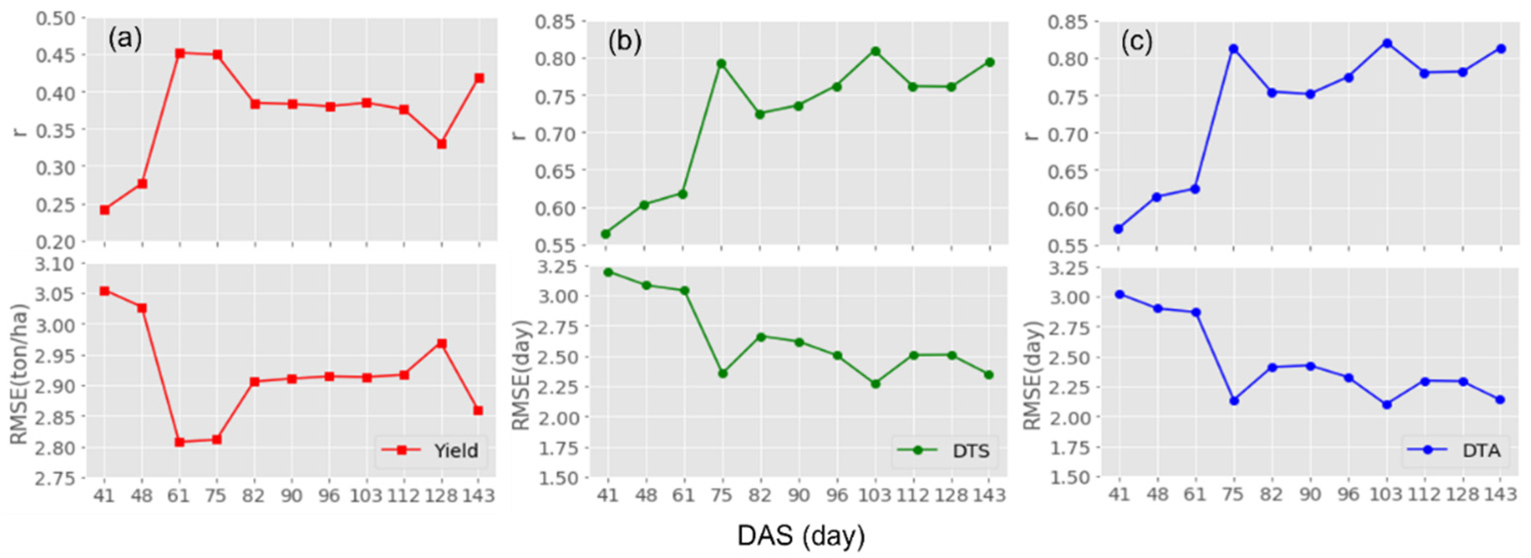
3.3. Model Performance by the UAV Survey Timing

Predicting flowering time and end-of-season yield as early as possible during the growing season is highly desirable for breeders and farmers to coordinate field work and possibly accelerate selection. To evaluate the potential of remotely sensed data in estimating maize yield and flowering time at early growth stages, the performance of ridge regression models (Figure 5) was compared when they were trained and validated with the full band spectral reflectance collected at the 11 dates. For yield estimation, the best accuracy was achieved with imagery at 61 DAS around the tasseling stage (VT) (Figure 5a). The VT stage is an important process for the determination of grain yield. It begins when the last branch of the tassel emerges from the whorl [95]. Before reaching the VT stage, maize plants quickly grow to the maximum height and accumulate dry matter. Some of the key traits regulating the final yield, such as the potential ovule number and ear size, have also been determined [96,97,98]. From the VT stage, the plant will shed its pollen at an approximate time as silk emerges. At this time, a few factors could greatly affect the success of fertilization and consequently influence the potential grain yield at harvest time. For example, inappropriate wind speed, air humidity, and temperature decrease the pollen shed. Moreover, the maize plants are most vulnerable to hail damage at the VT stage, as severe leaf loss at this time results in huge yield loss by harvest [99,100]. Therefore, significant physiological changes on the maize canopy relating to the end-of-season yield can be captured by the UAV imagery around the VT stage for the best yield estimation.
The relatively low accuracies (r < 0.3) at the 41 (V6–V8) and 48 DAS (V9–V11) indicated that these stages were too early for predicting maize yield using the UAV imagery. This is because, in the early growth stages before V11, the plant is still in the stage of nutrient accumulation and increasing leaf area. The yield potential was still developing and not accurately determined [101,102]. Additionally, the estimation performance started declining when entering the reproductive stages (75 DAS). This decreasing tendency was probably due to the canopy greenness alteration caused by the presence of well-developed tassels. Similar results were also reported in [102,103].
The model predictions for the DTS and DTA had a similar pattern (Figure 5b,c). The best results for both occurred at two critical time points, 75 DAS and 103 DAS, when the plants were at the R1 and R4 growth stages, respectively. The UAV survey date of 75 DAS was very close to the average DTS (69 DAS) and DTA (67 DAS) in the experiment. The flowering time was recorded for a maize plot when 50% of the plants in it displayed tassels or silks. Tassel and silk development change rapidly on a daily basis, and thus breeders have to visit each plot every other day during the flowering period. The variation in the flowering process among maize hybrids (i.e., some had more tassel branches or silks while some had fewer) was recorded by the image features collected during the process by averaging the image reflectance values of tassels or silks and vegetation. It was also reported that the BNDVI values had the highest correlations with the flowering time when they were collected slightly before the manually assessed flowering time (average for all genotypes) [36].
It was also noted that one UAV survey at the 103 DAS also reached good estimation performance post-flowering when all the tassels and silks were well developed. During this period, pollen grains that were received by silks quickly developed into pollen tubes that would penetrate the silk tissue and fertilize the ovules. Soon after the fertilization success, the silks dropped away, and the kernels started to develop. The substantial physiological changes that happened after the flowering process could be captured by the UAV imagery and used to infer back to the following time. Figure 6 shows canopy images of a maize plot collected at four growth stages. It is clearly seen that, as the plants developed, more tassels and silks were displayed in the plot and took up more pixels in the canopy images. At 103 DAS, almost all the plants had thoroughly displayed tassels and silks, and the substantial presence of the flowers during this period largely altered the maize canopy appearance. Consequently, this distinct canopy transformation provided a direct mechanism for flowering time prediction, resulting in higher estimation accuracy. Thus, it was observed in the experiment that the UAV survey timing for estimating the flowering time of maize hybrid could be flexible since the beginning of the flowering process, and we obtained the best estimates with imagery around the R1 and R4 stages.

4. Conclusions

In this study, a robust HTP framework was developed to estimate two important traits for large maize breeding populations, namely grain yield and flowering time. Four types of image features, i.e., reflectance, first and second derivatives of the full band spectra, and 81 narrow-band VIs, were extracted from the hyperspectral images collected along the growing season. Three machine learning models, i.e., ridge, SVR, and RF, were developed for the yield and flowering time estimation, and their performance with each of the four feature types was evaluated. The results showed that the ridge model achieved the highest prediction accuracy with the time-series reflectance features and outperformed the other models. Besides, the full band reflectance was the most effective feature type in the estimation regarding the correlations with ground data and model accuracy. Additionally, we evaluated the best UAV survey timing in the maize growing season to estimate these two traits. The results showed that the image features at the VT stage (61 DAS) had the best accuracy for maize grain yield estimation ( r = 0.51), and those collected at R1 (75 DAS) or R4 (103 DAS) had the estimation performance of r over 0.8 for both DTA and DTS.
The results of this study demonstrated the efficacy of using machine learning models and hyperspectral features for estimating critical agronomic traits of large maize breeding populations. The proposed HTP framework can allow maize breeders to efficiently phenotype breeding material in field trials and facilitate the decision-making process in the selection of superior genotypes with data-driven references. For future work, we plan to incorporate plant geometric features, genomic information, environmental data, and management practices to further facilitate estimation accuracy.

Author Contributions

Conceptualization, J.F., J.Z. and Z.Z.; data collection, D.C.L., N.d.L. and S.M.K.; methodology, J.F. and Z.Z.; validation, J.F., J.Z., B.W. and Z.Z.; data curation, B.W. and D.C.L.; writing—original draft, J.F., J.Z. and Z.Z.; writing—review and editing, J.F., J.Z., Z.Z., B.W., S.M.K., N.d.L. and D.C.L. All authors have read and agreed to the published version of the manuscript.

Funding

This research was supported by the USDA National Institute of Food and Agriculture, AFRI project accession No. 1028196; and Wisconsin Dairy Innovation Hub.

Conflicts of Interest

The authors declare no conflict of interest.

References

  1. Tilman, D.; Balzer, C.; Hill, J.; Befort, B.L. Global Food Demand and the Sustainable Intensification of Agriculture. Proc. Natl. Acad. Sci. USA 2011, 108, 20260–20264. [Google Scholar] [CrossRef] [PubMed] [Green Version]
  2. Prosekov, A.Y.; Ivanova, S.A. Food Security: The Challenge of the Present. Geoforum 2018, 91, 73–77. [Google Scholar] [CrossRef]
  3. Pingali, P. Westernization of Asian Diets and the Transformation of Food Systems: Implications for Research and Policy. Food Policy 2007, 32, 281–298. [Google Scholar] [CrossRef] [Green Version]
  4. Breene, K. Food Security and Why It Matters. Available online: https://www.weforum.org/agenda/2016/01/food-security-and-why-it-matters/ (accessed on 10 January 2022).
  5. Tscharntke, T.; Clough, Y.; Wanger, T.C.; Jackson, L.; Motzke, I.; Perfecto, I.; Vandermeer, J.; Whitbread, A. Global Food Security, Biodiversity Conservation and the Future of Agricultural Intensification. Biol. Conserv. 2012, 151, 53–59. [Google Scholar] [CrossRef]
  6. Phalan, B.; Onial, M.; Balmford, A.; Green, R.E. Reconciling Food Production and Biodiversity Conservation: Land Sharing and Land Sparing Compared. Science 2011, 333, 1289–1291. [Google Scholar] [CrossRef]
  7. Foley, J.A.; Ramankutty, N.; Brauman, K.A.; Cassidy, E.S.; Gerber, J.S.; Johnston, M.; Mueller, N.D.; O’Connell, C.; Ray, D.K.; West, P.C.; et al. Solutions for a Cultivated Planet. Nature 2011, 478, 337–342. [Google Scholar] [CrossRef] [Green Version]
  8. Phalan, B.; Balmford, A.; Green, R.E.; Scharlemann, J.P.W. Minimising the Harm to Biodiversity of Producing More Food Globally. Food Policy 2011, 36, S62–S71. [Google Scholar] [CrossRef]
  9. Tanumihardjo, S.A.; McCulley, L.; Roh, R.; Lopez-Ridaura, S.; Palacios-Rojas, N.; Gunaratna, N.S. Maize Agro-Food Systems to Ensure Food and Nutrition Security in Reference to the Sustainable Development Goals. Glob. Food Secur. 2020, 25, 100327. [Google Scholar] [CrossRef]
  10. Maize Production Quantity. Available online: https://knoema.com/atlas/topics/Agriculture/Crops-Production-Quantity-tonnes/Maize-production?type=maps (accessed on 10 January 2022).
  11. Bruce, W.B.; Edmeades, G.O.; Barker, T.C. Molecular and Physiological Approaches to Maize Improvement for Drought Tolerance. J. Exp. Bot. 2002, 53, 13–25. [Google Scholar] [CrossRef]
  12. Rajcan, I.; Swanton, C.J. Understanding Maize-Weed Competition: Resource Competition, Light Quality and the Whole Plant. Field Crops Res. 2001, 71, 139–150. [Google Scholar] [CrossRef]
  13. Yang, W.; Nigon, T.; Hao, Z.; Dias Paiao, G.; Fernández, F.G.; Mulla, D.; Yang, C. Estimation of Corn Yield Based on Hyperspectral Imagery and Convolutional Neural Network. Comput. Electron. Agric. 2021, 184, 106092. [Google Scholar] [CrossRef]
  14. Rouf Shah, T.; Prasad, K.; Kumar, P. Maize—A Potential Source of Human Nutrition and Health: A Review. Cogent Food Agric. 2016, 2, 1166995. [Google Scholar] [CrossRef]
  15. Shiferaw, B.; Prasanna, B.M.; Hellin, J.; Bänziger, M. Crops That Feed the World 6. Past Successes and Future Challenges to the Role Played by Maize in Global Food Security. Food Secur. 2011, 3, 307–327. [Google Scholar] [CrossRef] [Green Version]
  16. Poland, J. Breeding-Assisted Genomics. Curr. Opin. Plant Biol. 2015, 24, 119–124. [Google Scholar] [CrossRef] [PubMed]
  17. McMullen, M.D.; Kresovich, S.; Villeda, H.S.; Bradbury, P.; Li, H.; Sun, Q.; Flint-Garcia, S.; Thornsberry, J.; Acharya, C.; Bottoms, C.; et al. Genetic Properties of the Maize Nested Association Mapping Population. Science 2009, 325, 737–740. [Google Scholar] [CrossRef] [PubMed] [Green Version]
  18. Chivasa, W.; Mutanga, O.; Burgueño, J. UAV-Based High-Throughput Phenotyping to Increase Prediction and Selection Accuracy in Maize Varieties under Artificial MSV Inoculation. Comput. Electron. Agric. 2021, 184, 106128. [Google Scholar] [CrossRef]
  19. Pugh, N.A.; Horne, D.W.; Murray, S.C.; Carvalho, G.; Malambo, L.; Jung, J.; Chang, A.; Maeda, M.; Popescu, S.; Chu, T.; et al. Temporal Estimates of Crop Growth in Sorghum and Maize Breeding Enabled by Unmanned Aerial Systems. Plant Phenome J. 2018, 1, 1–10. [Google Scholar] [CrossRef]
  20. Li, L.; Zhang, Q.; Huang, D. A Review of Imaging Techniques for Plant Phenotyping. Sensors 2014, 14, 20078–20111. [Google Scholar] [CrossRef]
  21. Naik, H.S.; Zhang, J.; Lofquist, A.; Assefa, T.; Sarkar, S.; Ackerman, D.; Singh, A.; Singh, A.K.; Ganapathysubramanian, B. A Real-Time Phenotyping Framework Using Machine Learning for Plant Stress Severity Rating in Soybean. Plant Methods 2017, 13, 23. [Google Scholar] [CrossRef] [Green Version]
  22. Sankaran, S.; Zhou, J.; Khot, L.R.; Trapp, J.J.; Mndolwa, E.; Miklas, P.N. High-Throughput Field Phenotyping in Dry Bean Using Small Unmanned Aerial Vehicle Based Multispectral Imagery. Comput. Electron. Agric. 2018, 151, 84–92. [Google Scholar] [CrossRef]
  23. Singh, D.; Wang, X.; Kumar, U.; Gao, L.; Noor, M.; Imtiaz, M.; Singh, R.P.; Poland, J. High-Throughput Phenotyping Enabled Genetic Dissection of Crop Lodging in Wheat. Front. Plant Sci. 2019, 10, 394. [Google Scholar] [CrossRef] [PubMed] [Green Version]
  24. Qiu, Q.; Sun, N.; Bai, H.; Wang, N.; Fan, Z.; Wang, Y.; Meng, Z.; Li, B.; Cong, Y. Field-Based High-Throughput Phenotyping for Maize Plant Using 3d LIDAR Point Cloud Generated with a “Phenomobile”. Front. Plant Sci. 2019, 10, 554. [Google Scholar] [CrossRef] [PubMed] [Green Version]
  25. Fehr, W.R. Principles of Cultivar Development; Macmillan: New York, NY, USA, 1987. [Google Scholar]
  26. Lee, E.A.; Tracy, W.F. Handbook of Maize: Genetics and Genomics; Springer: New York, NY, USA, 2009; ISBN 9780387778624. [Google Scholar]
  27. Zhou, J.; Zhou, J.; Ye, H.; Ali, M.L.; Chen, P.; Nguyen, H.T. Yield Estimation of Soybean Breeding Lines under Drought Stress Using Unmanned Aerial Vehicle-Based Imagery and Convolutional Neural Network. Biosyst. Eng. 2021, 204, 90–103. [Google Scholar] [CrossRef]
  28. Moreira, F.F.; Hearst, A.A.; Cherkauer, K.A.; Rainey, K.M. Improving the Efficiency of Soybean Breeding with High-Throughput Canopy Phenotyping. Plant Methods 2019, 15, 139. [Google Scholar] [CrossRef] [PubMed]
  29. Sun, J.; Poland, J.A.; Mondal, S.; Crossa, J.; Juliana, P.; Singh, R.P.; Rutkoski, J.E.; Jannink, J.L.; Crespo-Herrera, L.; Velu, G.; et al. High-Throughput Phenotyping Platforms Enhance Genomic Selection for Wheat Grain Yield across Populations and Cycles in Early Stage. Theor. Appl. Genet. 2019, 132, 1705–1720. [Google Scholar] [CrossRef]
  30. Tanger, P.; Klassen, S.; Mojica, J.P.; Lovell, J.T.; Moyers, B.T.; Baraoidan, M.; Naredo, M.E.B.; McNally, K.L.; Poland, J.; Bush, D.R.; et al. Field-Based High Throughput Phenotyping Rapidly Identifies Genomic Regions Controlling Yield Components in Rice. Sci. Rep. 2017, 7, 42839. [Google Scholar] [CrossRef] [Green Version]
  31. Song, K.; Kim, H.C.; Shin, S.; Kim, K.H.; Moon, J.C.; Kim, J.Y.; Lee, B.M. Transcriptome Analysis of Flowering Time Genes under Drought Stress in Maize Leaves. Front. Plant Sci. 2017, 8, 267. [Google Scholar] [CrossRef] [Green Version]
  32. Buckler, E.S.; Holland, J.B.; Bradbury, P.J.; Acharya, C.B.; Brown, P.J.; Browne, C.; Ersoz, E.; Flint-Garcia, S.; Garcia, A.; Glaubitz, J.C.; et al. The Genetic Architecture of Maize Flowering Time. Science 2009, 325, 714–719. [Google Scholar] [CrossRef] [Green Version]
  33. Durand, E.; Bouchet, S.; Bertin, P.; Ressayre, A.; Jamin, P.; Charcosset, A.; Dillmann, C.; Tenaillon, M.I. Flowering Time in Maize: Linkage and Epistasis at a Major Effect Locus. Genetics 2012, 190, 1547–1562. [Google Scholar] [CrossRef] [Green Version]
  34. Franks, S.J. Plasticity and Evolution in Drought Avoidance and Escape in the Annual Plant Brassica rapa. New Phytol. 2011, 190, 249–257. [Google Scholar] [CrossRef]
  35. Andrade, F.H. Kernel Number Determination in Maize. Crop Sci. 1999, 39, 453–459. [Google Scholar] [CrossRef]
  36. Wu, G.; Miller, N.D.; de Leon, N.; Kaeppler, S.M.; Spalding, E.P. Predicting Zea mays Flowering Time, Yield, and Kernel Dimensions by Analyzing Aerial Images. Front. Plant Sci. 2019, 10, 1251. [Google Scholar] [CrossRef] [PubMed] [Green Version]
  37. Moghimi, A.; Yang, C.; Anderson, J.A. Aerial Hyperspectral Imagery and Deep Neural Networks for High-Throughput Yield Phenotyping in Wheat. Comput. Electron. Agric. 2020, 172, 105299. [Google Scholar] [CrossRef] [Green Version]
  38. Zhou, J.; Zhou, J.; Ye, H.; Ali, L.; Nguyen, H.T.; Chen, P. Classification of Soybean Leaf Wilting Due to Drought Stress Using UAV-Based Imagery. Comput. Electron. Agric. 2020, 175, 105576. [Google Scholar] [CrossRef]
  39. Gu, S.; Liao, Q.; Gao, S.; Kang, S.; Du, T.; Ding, R. Crop Water Stress Index as a Proxy of Phenotyping Maize Performance under Combined Water and Salt Stress. Remote Sens. 2021, 13, 4710. [Google Scholar] [CrossRef]
  40. Nikoli, A. Dynamics of Maize Vegetative Growth and Drought Adaptability Using Image-Based Phenotyping Under Controlled Conditions. Front. Plant Sci. 2021, 12, 571. [Google Scholar] [CrossRef]
  41. Guo, Y.; Wang, H.; Wu, Z.; Wang, S.; Sun, H.; Senthilnath, J.; Wang, J.; Bryant, C.R.; Fu, Y. Modified Red Blue Vegetation Index for Chlorophyll Estimation and Yield Prediction of Maize from Visible Images Captured by Uav. Sensors 2020, 20, 5055. [Google Scholar] [CrossRef]
  42. Peng, X.; Han, W.; Ao, J.; Wang, Y. Assimilation of Lai Derived from UAV Multispectral Data into the Safy Model to Estimate Maize Yield. Remote Sens. 2021, 13, 1094. [Google Scholar] [CrossRef]
  43. Quemada, M.; Gabriel, J.L.; Zarco-Tejada, P. Airborne Hyperspectral Images and Ground-Level Optical Sensors as Assessment Tools for Maize Nitrogen Fertilization. Remote Sens. 2014, 6, 2940–2962. [Google Scholar] [CrossRef] [Green Version]
  44. Danilevicz, M.F.; Bayer, P.E.; Boussaid, F.; Bennamoun, M.; Edwards, D. Maize Yield Prediction at an Early Developmental Stage Using Multispectral Images and Genotype Data for Preliminary Hybrid Selection. Remote Sens. 2021, 13, 3976. [Google Scholar] [CrossRef]
  45. Herrmann, I.; Bdolach, E.; Montekyo, Y.; Rachmilevitch, S.; Townsend, P.A.; Karnieli, A. Assessment of Maize Yield and Phenology by Drone-Mounted Superspectral Camera. Precis. Agric. 2020, 21, 51–76. [Google Scholar] [CrossRef]
  46. Peñuelas, J.; Filella, L. Technical Focus: Visible and near-Infrared Reflectance Techniques for Diagnosing Plant Physiological Status. Trends Plant Sci. 1998, 3, 151–156. [Google Scholar] [CrossRef]
  47. Babar, M.A.; Reynolds, M.P.; Van Ginkel, M.; Klatt, A.R.; Raun, W.R.; Stone, M.L. Spectral Reflectance to Estimate Genetic Variation for In-Season Biomass, Leaf Chlorophyll, and Canopy Temperature in Wheat. Crop Sci. 2006, 46, 1046–1057. [Google Scholar] [CrossRef]
  48. Schweiger, A.K.; Cavender-Bares, J.; Townsend, P.A.; Hobbie, S.E.; Madritch, M.D.; Wang, R.; Tilman, D.; Gamon, J.A. Plant Spectral Diversity Integrates Functional and Phylogenetic Components of Biodiversity and Predicts Ecosystem Function. Nat. Ecol. Evol. 2018, 2, 976–982. [Google Scholar] [CrossRef] [PubMed]
  49. Kycko, M.; Zagajewski, B.; Lavender, S.; Romanowska, E.; Zwijacz-Kozica, M. The Impact of Tourist Traffic on the Condition and Cell Structures of Alpine Swards. Remote Sens. 2018, 10, 220. [Google Scholar] [CrossRef] [Green Version]
  50. Yoosefzadeh-Najafabadi, M.; Earl, H.J.; Tulpan, D.; Sulik, J.; Eskandari, M. Application of Machine Learning Algorithms in Plant Breeding: Predicting Yield From Hyperspectral Reflectance in Soybean. Front. Plant Sci. 2021, 11, 624273. [Google Scholar] [CrossRef]
  51. Gao, S.; Niu, Z.; Huang, N.; Hou, X. Estimating the Leaf Area Index, Height and Biomass of Maize Using HJ-1 and RADARSAT-2. Int. J. Appl. Earth Obs. Geoinf. 2013, 24, 1–8. [Google Scholar] [CrossRef]
  52. Gnyp, M.L.; Miao, Y.; Yuan, F.; Ustin, S.L.; Yu, K.; Yao, Y.; Huang, S.; Bareth, G. Hyperspectral Canopy Sensing of Paddy Rice Aboveground Biomass at Different Growth Stages. Field Crops Res. 2014, 155, 42–55. [Google Scholar] [CrossRef]
  53. Fu, Y.; Yang, G.; Wang, J.; Song, X.; Feng, H. Winter Wheat Biomass Estimation Based on Spectral Indices, Band Depth Analysis and Partial Least Squares Regression Using Hyperspectral Measurements. Comput. Electron. Agric. 2014, 100, 51–59. [Google Scholar] [CrossRef]
  54. Kross, A.; McNairn, H.; Lapen, D.; Sunohara, M.; Champagne, C. Assessment of RapidEye Vegetation Indices for Estimation of Leaf Area Index and Biomass in Corn and Soybean Crops. Int. J. Appl. Earth Obs. Geoinf. 2015, 34, 235–248. [Google Scholar] [CrossRef] [Green Version]
  55. Feng, L.; Zhang, Z.; Ma, Y.; Du, Q.; Williams, P.; Drewry, J.; Luck, B. Alfalfa Yield Prediction Using UAV-Based Hyperspectral Imagery and Ensemble Learning. Remote Sens. 2020, 12, 2028. [Google Scholar] [CrossRef]
  56. Thorp, K.R.; Wang, G.; Bronson, K.F.; Badaruddin, M.; Mon, J. Hyperspectral Data Mining to Identify Relevant Canopy Spectral Features for Estimating Durum Wheat Growth, Nitrogen Status, and Grain Yield. Comput. Electron. Agric. 2017, 136, 1–12. [Google Scholar] [CrossRef] [Green Version]
  57. Tsai, F.; Philpot, W. Derivative Analysis of Hyperspectral Data. Remote Sens. Environ. 1998, 66, 41–51. [Google Scholar] [CrossRef]
  58. Tsai, F.; Philpot, W.D. A Derivative-Aided Hyperspectral Image Analysis System for Land-Cover Classification. IEEE Trans. Geosci. Remote Sens. 2002, 40, 416–425. [Google Scholar] [CrossRef]
  59. Bao, J.; Chi, M.; Benediktsson, J.A. Spectral Derivative Features for Classification of Hyperspectral Remote Sensing Images: Experimental Evaluation. IEEE J. Sel. Top. Appl. Earth Obs. Remote Sens. 2013, 6, 594–601. [Google Scholar] [CrossRef]
  60. Kalluri, H.R.; Prasad, S.; Bruce, L.M. Decision-Level Fusion of Spectral Reflectance and Derivative Information for Robust Hyperspectral Land Cover Classification. IEEE Trans. Geosci. Remote Sens. 2010, 48, 4047–4058. [Google Scholar] [CrossRef]
  61. Smith, K.L.; Steven, M.D.; Colls, J.J. Use of Hyperspectral Derivative Ratios in the Red-Edge Region to Identify Plant Stress Responses to Gas Leaks. Remote Sens. Environ. 2004, 92, 207–217. [Google Scholar] [CrossRef]
  62. Thorp, K.R.; Tian, L.; Yao, H.; Tang, L. Narrow-Band and Derivative-Based Vegetation Indices for Hyperspectral Data. Trans. ASAE 2004, 47, 291–299. [Google Scholar] [CrossRef]
  63. Savitzky, A.; Golay, M.J.E. Smoothing and Differentiation. Anal. Chem 1964, 36, 1627–1639. [Google Scholar] [CrossRef]
  64. Hoerl, A.E.; Kennard, R.W. Ridge Regression: Biased Estimation for Nonorthogonal Problems. Technometrics 1970, 12, 55–67. [Google Scholar] [CrossRef]
  65. Vogt, W. Ridge Regression. In Dictionary of Statistics and Methodology; Sage: New York, NY, USA, 2015; pp. 1–20. [Google Scholar] [CrossRef]
  66. Vapnik, V. The Nature of Statistical Learning Theory; Springer: New York, NY, USA, 2013. [Google Scholar]
  67. Auria, L.; Moro, R.A. Support Vector Machines (SVM) as a Technique for Solvency Analysis. SSRN Electron. J. 2011. [Google Scholar] [CrossRef] [Green Version]
  68. Drucker, H.; Surges, C.J.C.; Kaufman, L.; Smola, A.; Vapnik, V. Support Vector Regression Machines. Adv. Neural Inf. Process. Syst. 1997, 1, 155–161. [Google Scholar]
  69. Breiman, L. Random Forests. Mach. Learn. 2001, 45, 5–32. [Google Scholar] [CrossRef] [Green Version]
  70. Wang, L.; Zhou, X.; Zhu, X.; Dong, Z.; Guo, W. Estimation of Biomass in Wheat Using Random Forest Regression Algorithm and Remote Sensing Data. Crop J. 2016, 4, 212–219. [Google Scholar] [CrossRef] [Green Version]
  71. Wang, Y.; Zhang, Z.; Feng, L.; Du, Q. Combining Multi-Source Data and Machine Learning Approaches to Predict Winter Wheat Yield in The. Remote Sens. 2020, 12, 1232. [Google Scholar] [CrossRef] [Green Version]
  72. Ma, J.; Li, Y.; Chen, Y.; Du, K.; Zheng, F.; Zhang, L.; Sun, Z. Estimating above Ground Biomass of Winter Wheat at Early Growth Stages Using Digital Images and Deep Convolutional Neural Network. Eur. J. Agron. 2019, 103, 117–129. [Google Scholar] [CrossRef]
  73. Feng, L.; Wang, Y.; Zhang, Z.; Du, Q. Geographically and Temporally Weighted Neural Network for Winter Wheat Yield Prediction. Remote Sens. Environ. 2021, 262, 112514. [Google Scholar] [CrossRef]
  74. Feng, L.; Zhang, Z.; Ma, Y.; Sun, Y.; Du, Q.; Williams, P.; Drewry, J.; Luck, B. Multitask Learning of Alfalfa Nutritive Value From UAV-Based Hyperspectral Images. IEEE Geosci. Remote Sens. Lett. 2021, 19, 1–5. [Google Scholar] [CrossRef]
  75. Masjedi, A.; Crawford, M.M.; Carpenter, N.R.; Tuinstra, M.R. Multi-Temporal Predictive Modelling of Sorghum Biomass Using UAV-Based Hyperspectral and LiDAR Data. Remote Sens. 2020, 12, 3587. [Google Scholar] [CrossRef]
  76. Zhou, J.; Ye, H.; Nguyen, H.; Chen, P.; Zhou, J. Yield Estimation of Soybean Breeding Lines Using UAV Multispectral Imagery and Convolutional Neuron Network Jing. In Proceedings of the 2020 ASABE Annual International Virtual Meeting, Virtual, 13–15 July 2020; pp. 2–14. [Google Scholar]
  77. Gutierrez-Rodriguez, M.; Escalante-Estrada, J.A.; Rodriguez-Gonzalez, M.T. Canopy Reflectance, Stomatal Conductance, and Yield of Phaseolus vulgaris L. and Phaseolus coccinues L. Under Saline Field Conditions. Int. J. Agric. Biol. 2005, 7, 491–494. [Google Scholar]
  78. Candiago, S.; Remondino, F.; De Giglio, M.; Dubbini, M.; Gattelli, M. Evaluating Multispectral Images and Vegetation Indices for Precision Farming Applications from UAV Images. Remote Sens. 2015, 7, 4026–4047. [Google Scholar] [CrossRef] [Green Version]
  79. Condorelli, G.E.; Maccaferri, M.; Newcomb, M.; Andrade-Sanchez, P.; White, J.W.; French, A.N.; Sciara, G.; Ward, R.; Tuberosa, R. Comparative Aerial and Ground Based High Throughput Phenotyping for the Genetic Dissection of NDVI as a Proxy for Drought Adaptive Traits in Durum Wheat. Front. Plant Sci. 2018, 9, 893. [Google Scholar] [CrossRef] [PubMed]
  80. Shen, M.; Chen, J.; Zhu, X.; Tang, Y. Yellow Flowers Can Decrease NDVI and EVI Values: Evidence from a Field Experiment in an Alpine Meadow. Can. J. Remote Sens. 2009, 35, 99–106. [Google Scholar] [CrossRef]
  81. Shen, M.; Chen, J.; Zhu, X.; Tang, Y.; Chen, X. Do Flowers Affect Biomass Estimate Accuracy from NDVI and EVI? Int. J. Remote Sens. 2010, 31, 2139–2149. [Google Scholar] [CrossRef]
  82. Bernardo, R. Parental Selection, Number of Breeding Populations, and Size of Each Population in Inbred Development. Theor. Appl. Genet. 2003, 107, 1252–1256. [Google Scholar] [CrossRef]
  83. Rogers, A.R.; Dunne, J.C.; Romay, C.; Bohn, M.; Buckler, E.S.; Ciampitti, I.A.; Edwards, J.; Ertl, D.; Flint-Garcia, S.; Gore, M.A.; et al. The Importance of Dominance and Genotype-by-Environment Interactions on Grain Yield Variation in a Large-Scale Public Cooperative Maize Experiment. G3 Genes Genomes Genet. 2021, 11, jkaa050. [Google Scholar] [CrossRef]
  84. Kumar, A.; Rajalakshmi, P.; Guo, W.; Naik, B.B.; Marathi, B.; Desai, U.B. Detection and Counting of Tassels for Maize Crop Monitoring Using Multispectral Images. In Proceedings of the 2020 IEEE International Conference on Computing, Power and Communication Technologies (GUCON), Greater Noida, India, 2–4 October 2020; pp. 789–793. [Google Scholar] [CrossRef]
  85. Lambert, R.J.; Johnson, R.R. Leaf Angle, Tassel Morphology, and the Performance of Maize Hybrids 1. Crop Sci. 1978, 18, 499–502. [Google Scholar] [CrossRef]
  86. Hunter, R.B.; Daynard, T.B.; Hume, D.J.; Tanner, J.W.; Curtis, J.D.; Kannenberg, L.W. Effect of Tassel Removal on Grain Yield of Corn (Zea mays L.) 1. Crop Sci. 1969, 9, 405–406. [Google Scholar] [CrossRef]
  87. Gage, J.L.; Miller, N.D.; Spalding, E.P.; Kaeppler, S.M.; de Leon, N. TIPS: A System for Automated Image-Based Phenotyping of Maize Tassels. Plant Methods 2017, 13, 21. [Google Scholar] [CrossRef] [Green Version]
  88. Sun, C.; Feng, L.; Zhang, Z.; Ma, Y.; Crosby, T.; Naber, M.; Wang, Y. Prediction of End-of-Season Tuber Yield and Tuber Set in Potatoes Using in-Season Uav-Based Hyperspectral Imagery and Machine Learning. Sensors 2020, 20, 5293. [Google Scholar] [CrossRef]
  89. Thenkabail, P.S.; Smith, R.B.; De Pauw, E. Hyperspectral Vegetation Indices and Their Relationships with Agricultural Crop Characteristics. Remote Sens. Environ. 2000, 71, 158–182. [Google Scholar] [CrossRef]
  90. Myneni, R.B.; Williams, D.L. On the Relationship between FAPAR and NDVI. Remote Sens. Environ. 1994, 49, 200–211. [Google Scholar] [CrossRef]
  91. Prabhakara, K.; Hively, W.D.; Mccarty, G.W. Evaluating the Relationship between Biomass, Percent Groundcover and Remote Sensing Indices across Six Winter Cover Crop Fields in Maryland, United States. Int. J. Appl. Earth Obs. Geoinf. 2015, 39, 88–102. [Google Scholar] [CrossRef] [Green Version]
  92. Viña, A.; Leavitt, B.; Rundquist, D.C.; Keydan, G.; Leavitt, B.; Schepers, J. Monitoring Maize (Zea mays L.) Phenology with Remote Sensing. Agron. J. 2004, 96, 1139–1147. [Google Scholar] [CrossRef]
  93. Tesfaye, A.A. Evaluation of the Saturation Property of Vegetation Indices Derived from Sentinel-2 in Mixed Crop-Forest Ecosystem. Spat. Inf. Res. 2021, 29, 109–121. [Google Scholar] [CrossRef]
  94. Gitelson, A.A. Wide Dynamic Range Vegetation Index for Remote Quantification of Biophysical Characteristics of Vegetation. J. Plant Physiol. 2004, 161, 165–173. [Google Scholar] [CrossRef] [Green Version]
  95. Abendroth, L.J.; Elmore, R.W.; Boyer, M.J.; Marlay, S.K. Corn Growth and Development; Iowa State University: Ames, IA, USA, 2011. [Google Scholar]
  96. Nielsen, R.L. Ear Size Determination in Corn. Available online: https://www.agry.purdue.edu/ext/corn/news/timeless/EarSize.html (accessed on 10 January 2022).
  97. Hanway, J.J. How a Corn Plant Develops; Special Report; Iowa Agricultural and Home Economics Experiment State Publications: Ames, IA, USA, 1966; Volume 48, pp. 1–18. [Google Scholar]
  98. Nielsen, R.L. Grain Fill Stages in Corn. Available online: https://www.agry.purdue.edu/ext/corn/news/timeless/grainfill.html (accessed on 10 January 2022).
  99. Nleya, T.; Chungu, C.; Kleinjan, J. Corn Growth and Development. In Best Management Practices; South Dakota University: Brookings, SD, USA, 2016. [Google Scholar]
  100. Ransom, J.; Endres, G. Corn: Growth and Management Quick Guide: Revised; North Dakota State University: Fargo, ND, USA, 2020; Volume 1173, pp. 1–8. [Google Scholar]
  101. Teal, R.; Tubana, B.; Arnall, B.; Walsh, O. In-Season Prediction of Corn Grain Yield Potential Using Normalized Difference Vegetation Index. Agron. J. 2006, 98, 1488–1494. [Google Scholar] [CrossRef] [Green Version]
  102. Zhang, M.; Michael, O.; Hendley, P.; Drost, D. Corn and Soybean Yield Indicators Using Remotely Sensed Vegetation Index. In Proceedings of the Fourth International Conference on Precision Agriculture, St. Paul, MN, USA, 19–22 July 1998; American Society of Agronomy, Crop Science Society of America, Soil Science Society of America: Madison, WI, USA, 1999; pp. 1475–1481. [Google Scholar]
  103. Spitkó, T.; Nagy, Z.; Zsubori, Z.T.; Szőke, C.; Berzy, T.; Pintér, J.; Marton, C.L. Connection between Normalized Difference Vegetation Index and Yield in Maize. Plant Soil Environ. 2016, 62, 293–298. [Google Scholar] [CrossRef]
Figure 1. Maize breeding experimental trial at AARS.
Remotesensing 14 03052 g001
Figure 2. Box plots of the ground truth field data.
Remotesensing 14 03052 g002
Figure 3. Spectral profiles of the hybrids with the top 10% and bottom 10% yields in the 400–700 nm (a,d,g), 700–800 nm (b,e,h), and 800–1000 nm (c,f,i) wavelength ranges at the early (ac), middle (df), and late (gi) growth stages.
Remotesensing 14 03052 g003
Figure 4. Pearson correlations between the spectral information and maize grain yield. The correlations were calculated for each spectral band at individual data collections. The averaged correlations over all the dates are shown in the plot.
Remotesensing 14 03052 g004
Figure 5. Line chart of the Pearson correlation coefficients (r) and RMSE between the observed and predicted (a) yield, (b) DTS, and (c) DTA using the full band spectral reflectance along the growing season.
Remotesensing 14 03052 g005
Figure 6. Canopy images of a maize plot at (a) the V6–V8 stage (41 DAS), (b) the VT stage (61 DAS), (c) the R1 stage (75 DAS), (d) the R3 stage (90 DAS), and (e) the R4 stage (103 DAS). The images were taken by the hyperspectral camera at a 42 m height and composited using the red (620 nm), green (530 nm), and blue (465 nm) bands from the hyperspectral imagery. Red boxes highlight the tassel parts on the maize canopy.
Remotesensing 14 03052 g006
Table 1. UAV survey dates, days after seeding, and growth stages.
Flight DatesDASGrowth Stages
23 June41V6–V8 (6–8 Leaf Collars)
30 June48V9–V11 (9–11 Leaf Collars)
13 July61VT (Tasseling)
27 July75R1 (Silking)
3 August82R2 (Blister)
11 August90R3 (Milk)
17 August96R4 (Dough)
24 August103R4 (Dough)
2 September112R5 (Dent)
18 September128R5 (Dent)
3 October143R6 (Black Layer)
Table 2. Paired sample t-test results between the top 10% and bottom 10% yield groups.
Growth StagesRegiontp-Value
Early Stages, 48 DAS400–700 nm−1.5690910.117789
700–800 nm−0.4866460.627719
800–100 nm−4.4901460.000013
Middle Stages, 96 DAS400–700 nm−0.7554780.450616
700–800 nm−0.5949240.553421
800–100 nm−5.7090190.000000
Late Stages, 112 DAS400–700 nm0.1911380.848560
700–800 nm−0.3233030.747233
800–100 nm−3.7637160.000226
Table 3. Performance of the ridge, SVR, and RF models in maize yield and flowering time estimation using the combined 11-day features. The numbers outside the parenthesis show the averaged accuracies of the repeated four-fold cross-validation, and the numbers in the parenthesis are standard deviations of the repeated testing accuracies.
Phenotypic DataModelFeaturesMetrics
rMAERMSE
Yield
(ton/ha)
RidgeFull Band Spectral Reflectance0.542.102.68
(0.01)(0.02)(0.03)
First Derivatives of Full Bands0.412.743.51
(0.01)(0.03)(0.04)
Second Derivatives of Full Bands0.372.973.78
(0.02)(0.05)(0.06)
81 Vegetation Indices0.152.5512.26
(0.09)(0.42)(14.88)
SVRFull Band Spectral Reflectance0.532.102.69
(0.01)(0.02)(0.02)
First Derivatives of Full Bands0.492.302.95
(0.01)(0.03)(0.04)
Second Derivatives of Full Bands0.452.413.08
(0.01)(0.03)(0.05)
81 Vegetation Indices0.472.132.91
(0.01)(0.02)(0.05)
RFFull Band Spectral Reflectance0.442.332.83
(0.01)(0.01)(0.01)
First Derivatives of Full Bands0.482.292.78
(0.01)(0.01)(0.01)
Second Derivatives of Full Bands0.462.342.82
(0.01)(0.01)(0.01)
81 Vegetation Indices0.462.302.80
(0.01)(0.01)(0.01)
DTS
(day)
RidgeFull Band Spectral Reflectance0.911.271.63
(<0.01)(0.01)(0.01)
First Derivatives of Full Bands0.861.602.05
(<0.01)(0.03)(0.03)
Second Derivatives of Full Bands0.821.842.34
(0.01)(0.02)(0.03)
81 Vegetation Indices0.241.9017.40
(0.10)(0.34)(12.24)
SVRFull Band Spectral Reflectance0.891.351.76
(<0.01)(0.02)(0.03)
First Derivatives of Full Bands0.891.421.81
(<0.01)(0.02)(0.03)
Second Derivatives of Full Bands0.861.572.02
(<0.01)(0.02)(0.03)
81 Vegetation Indices0.741.422.99
(0.05)(0.04)(0.48)
RFFull Band Spectral Reflectance0.841.592.12
(0.01)(0.01)(0.03)
First Derivatives of Full Bands0.851.542.02
(<0.01)(0.01)(0.02)
Second Derivatives of Full Bands0.831.632.20
(0.01)(0.02)(0.03)
81 Vegetation Indices0.861.501.96
(<0.01)(0.01)(0.01)
DTA
(day)
RidgeFull Band Spectral Reflectance0.921.161.48
(<0.01)(0.01)(0.01)
First Derivatives of Full Bands0.871.491.89
(<0.01)(0.03)(0.04)
Second Derivatives of Full Bands0.841.632.07
(<0.01)(0.03)(0.02)
81 Vegetation Indices0.431.5410.18
(0.22)(0.27)(9.29)
SVRFull Band Spectral Reflectance0.901.241.61
(<0.01)(0.02)(0.03)
First Derivatives of Full Bands0.891.321.69
(<0.01)(0.01)(0.02)
Second Derivatives of Full Bands0.871.421.81
(<0.01)(0.02)(0.03)
81 Vegetation Indices0.791.272.45
(0.04)(0.03)(0.29)
RFFull Band Spectral Reflectance0.851.481.97
(0.01)(0.01)(0.03)
First Derivatives of Full Bands0.871.391.84
(<0.01)(0.01)(0.02)
Second Derivatives of Full Bands0.841.522.04
(<0.01)(0.01)(0.02)
81 Vegetation Indices0.881.351.78
(<0.01)(0.01)(0.02)
Publisher’s Note: MDPI stays neutral with regard to jurisdictional claims in published maps and institutional affiliations.

