Temporal Coherence Estimators for GBSAR


Abstract
:1. Introduction
2. Materials and Methods
2.1. The Coherence Estimator
2.2. The Amplitude Dispersion Index
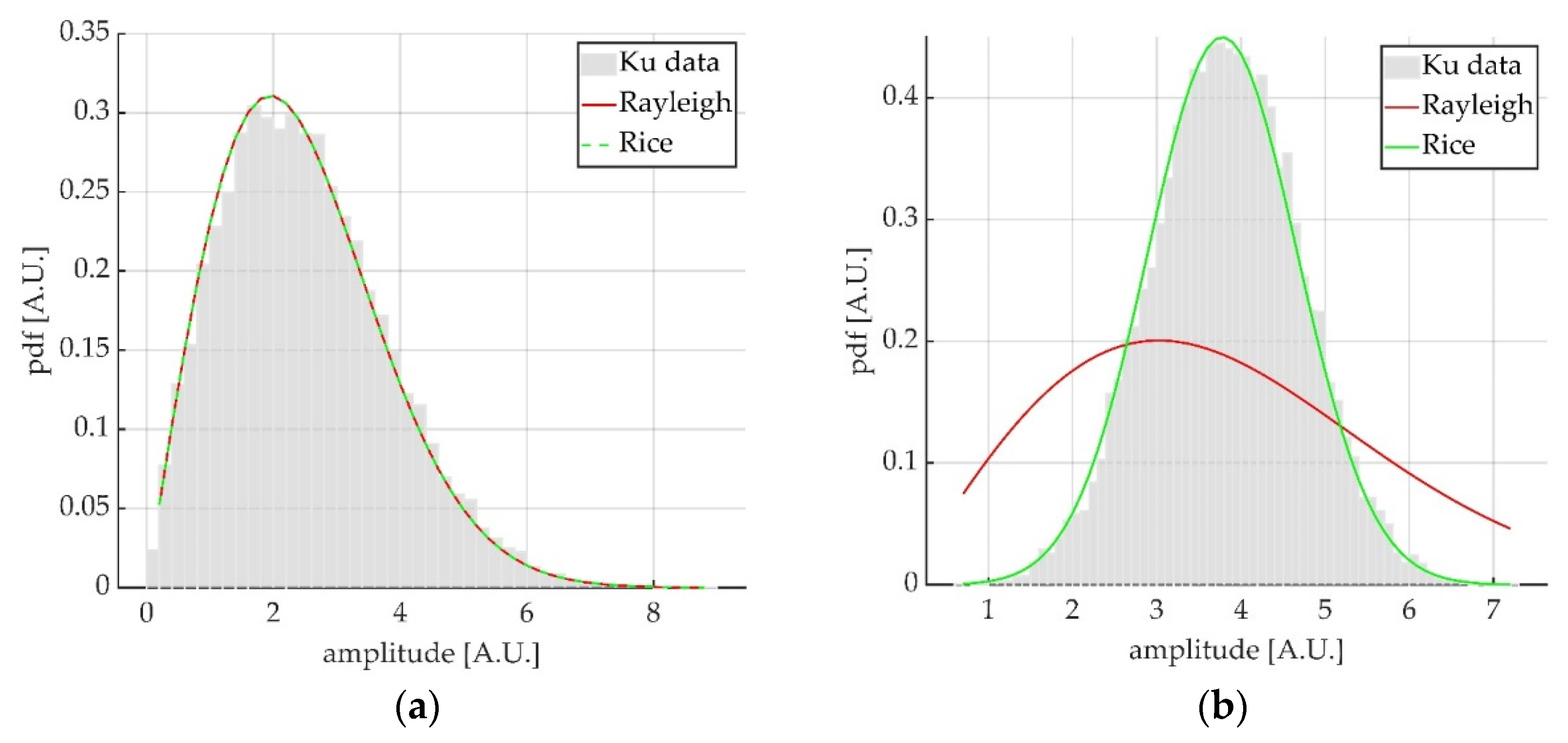
2.3. Amplitude Statistics of Radar Data
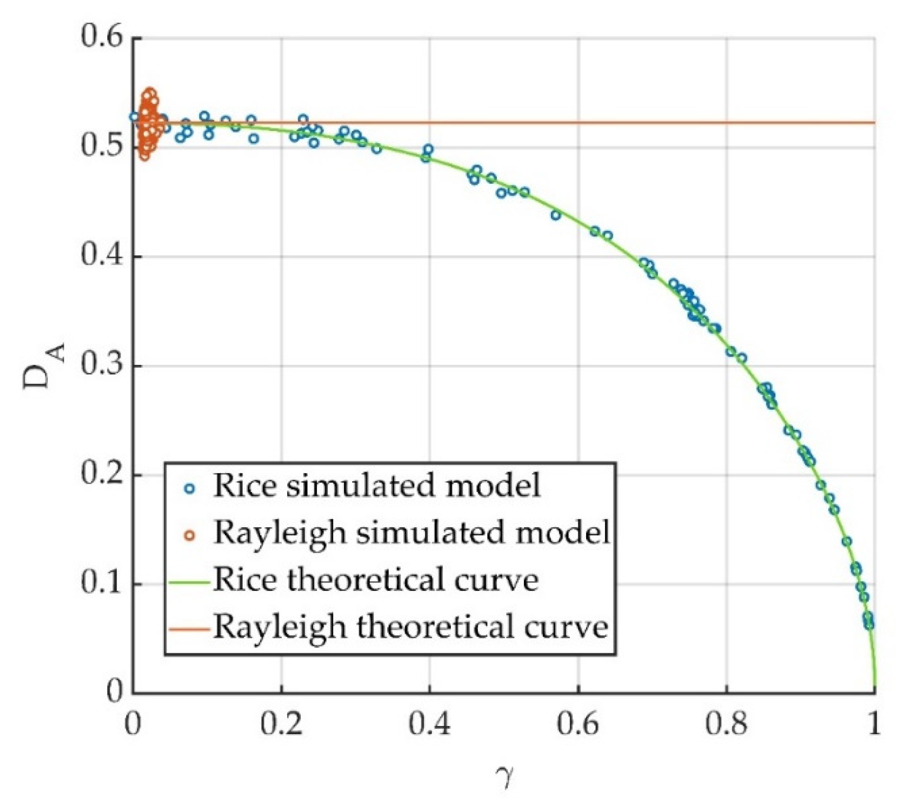
2.4. Relation between Amplitude Dispersion Index and Coherence
2.5. Simulations
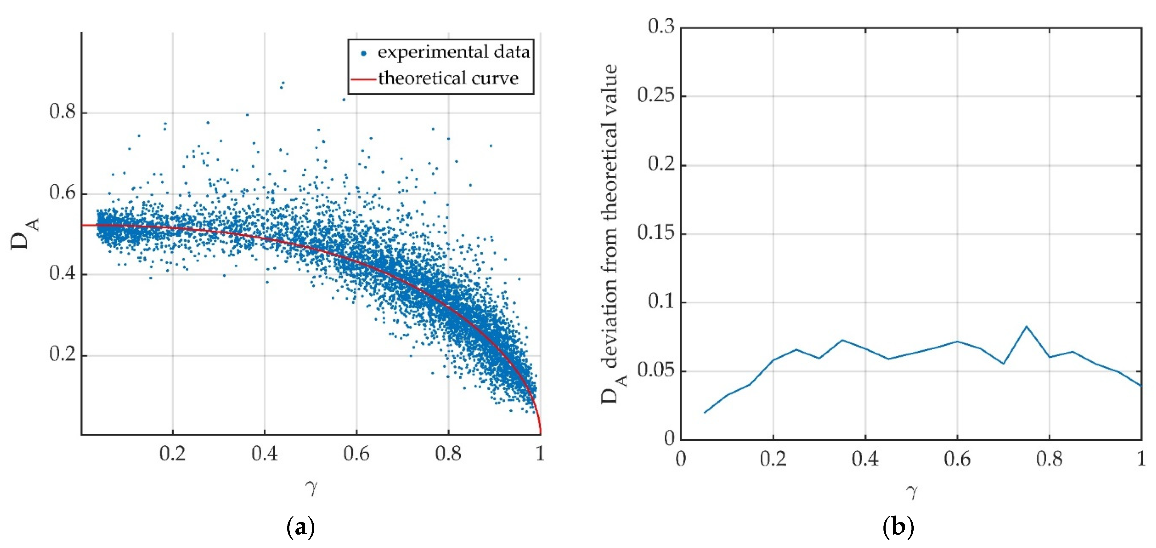
3. Results
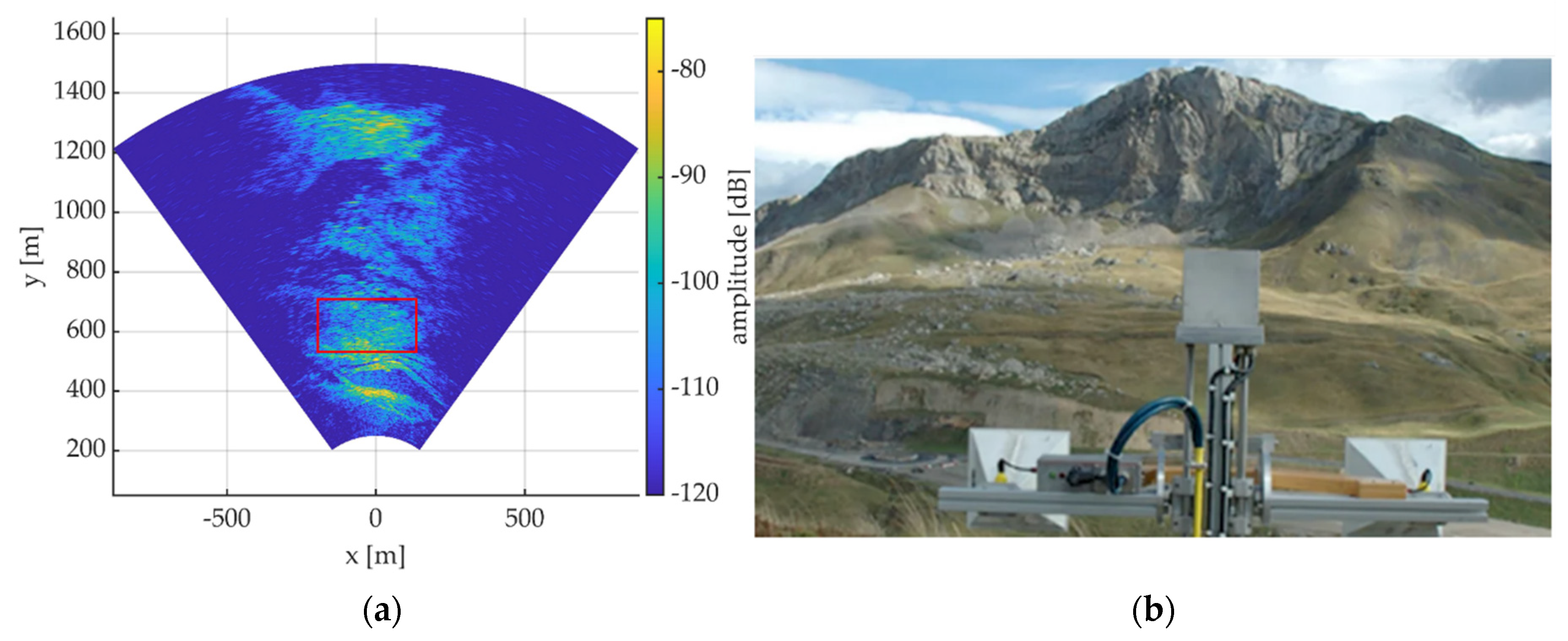
3.1. Formigal Measurement Campaign
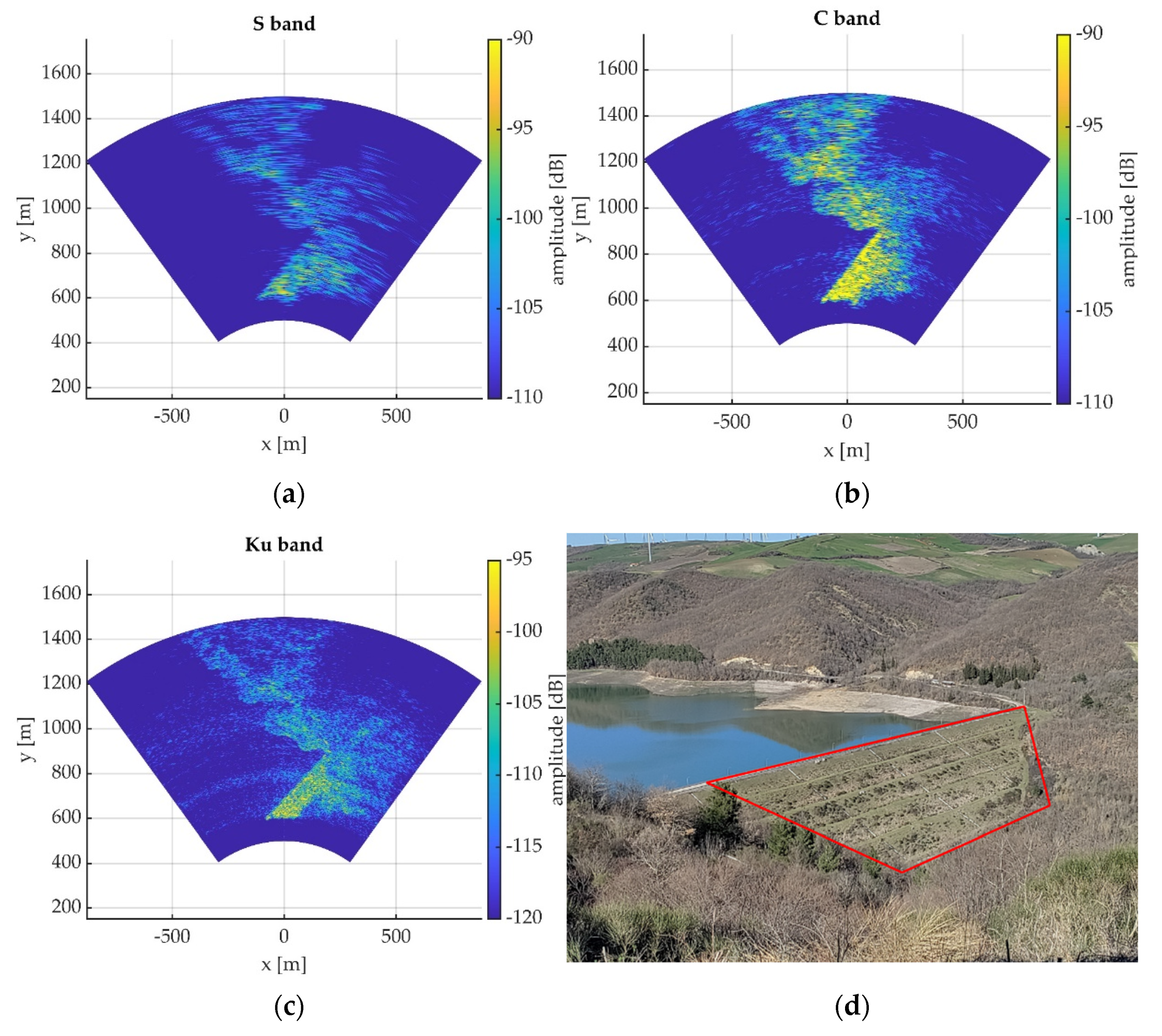
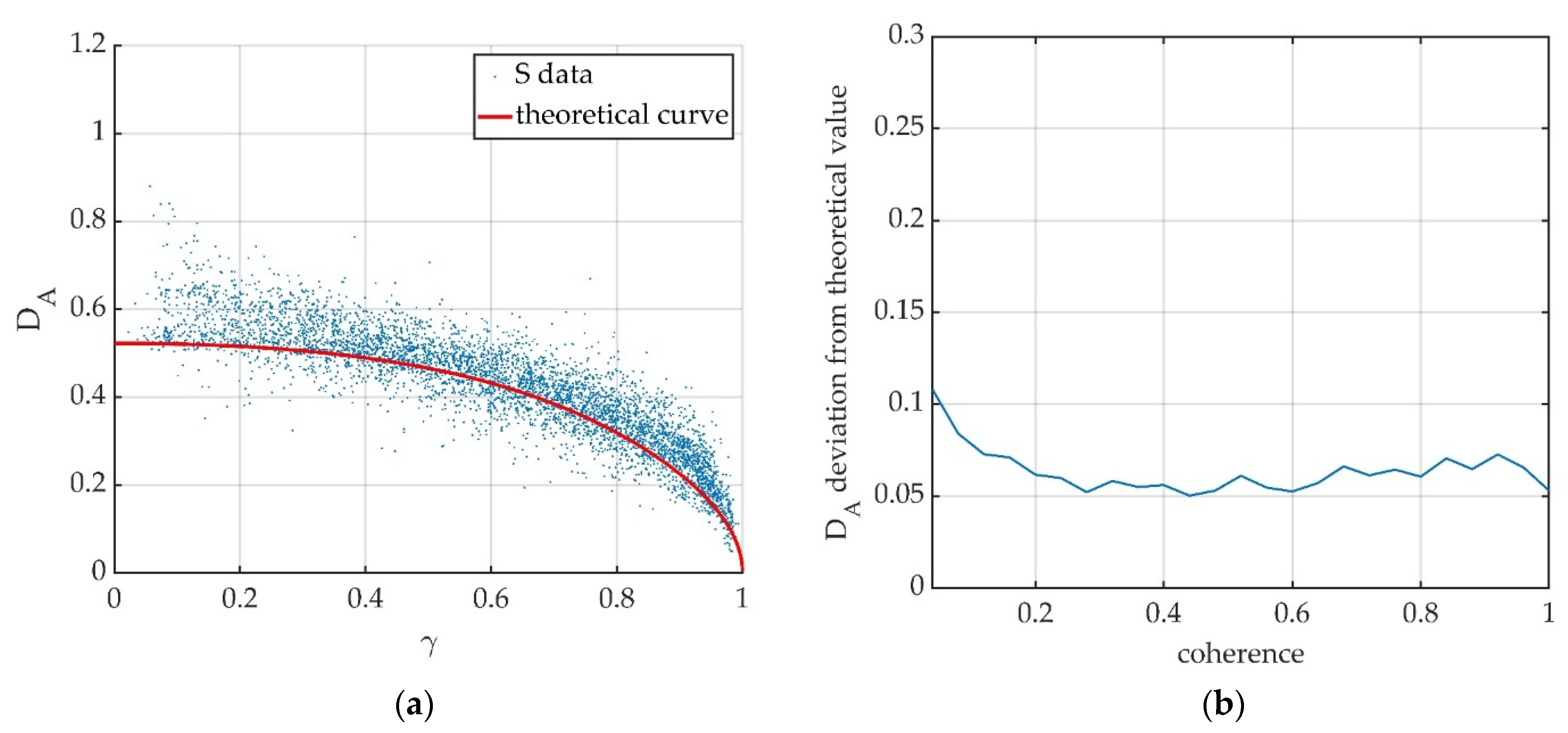
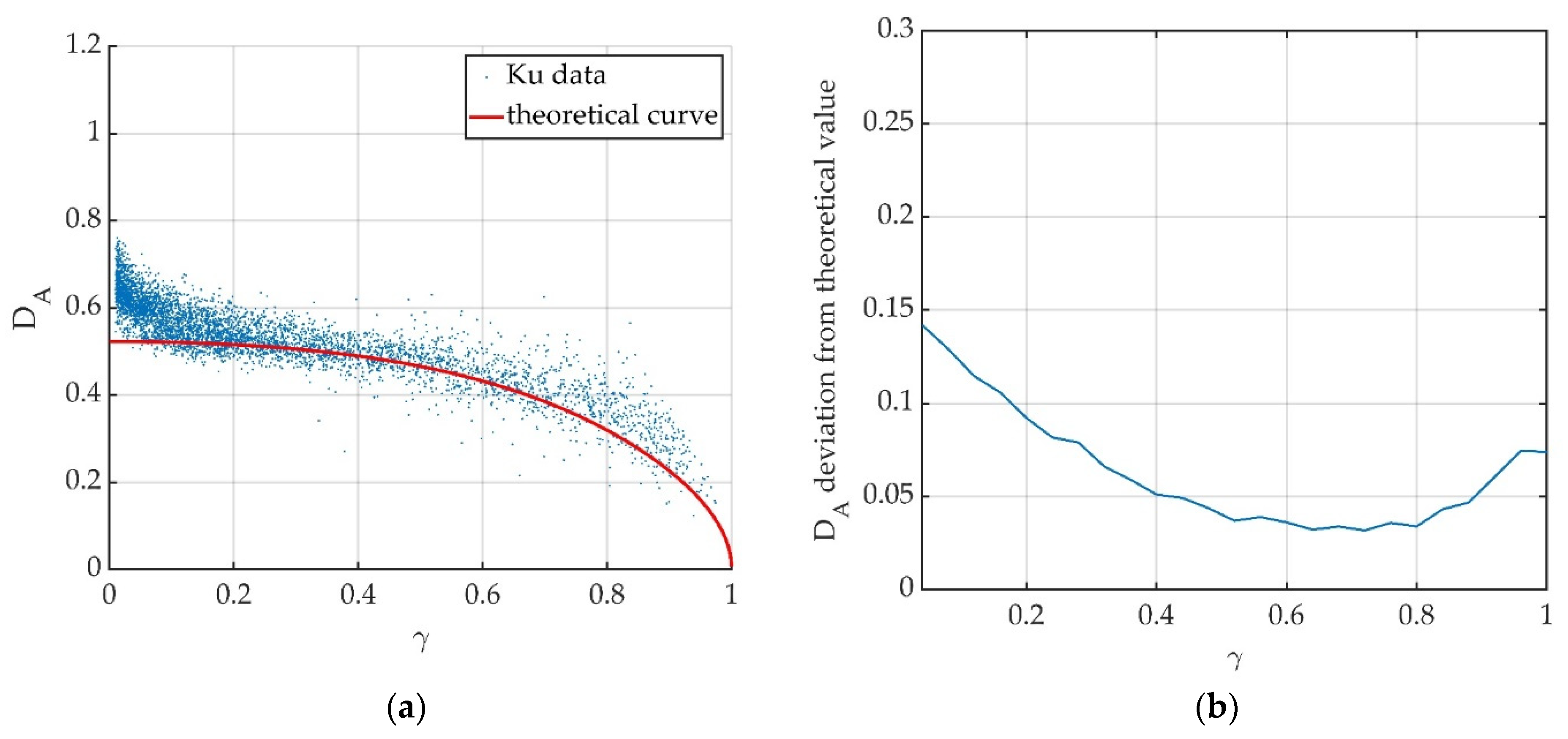
3.2. Aquilonia Test Site: Validation with Different Frequencies
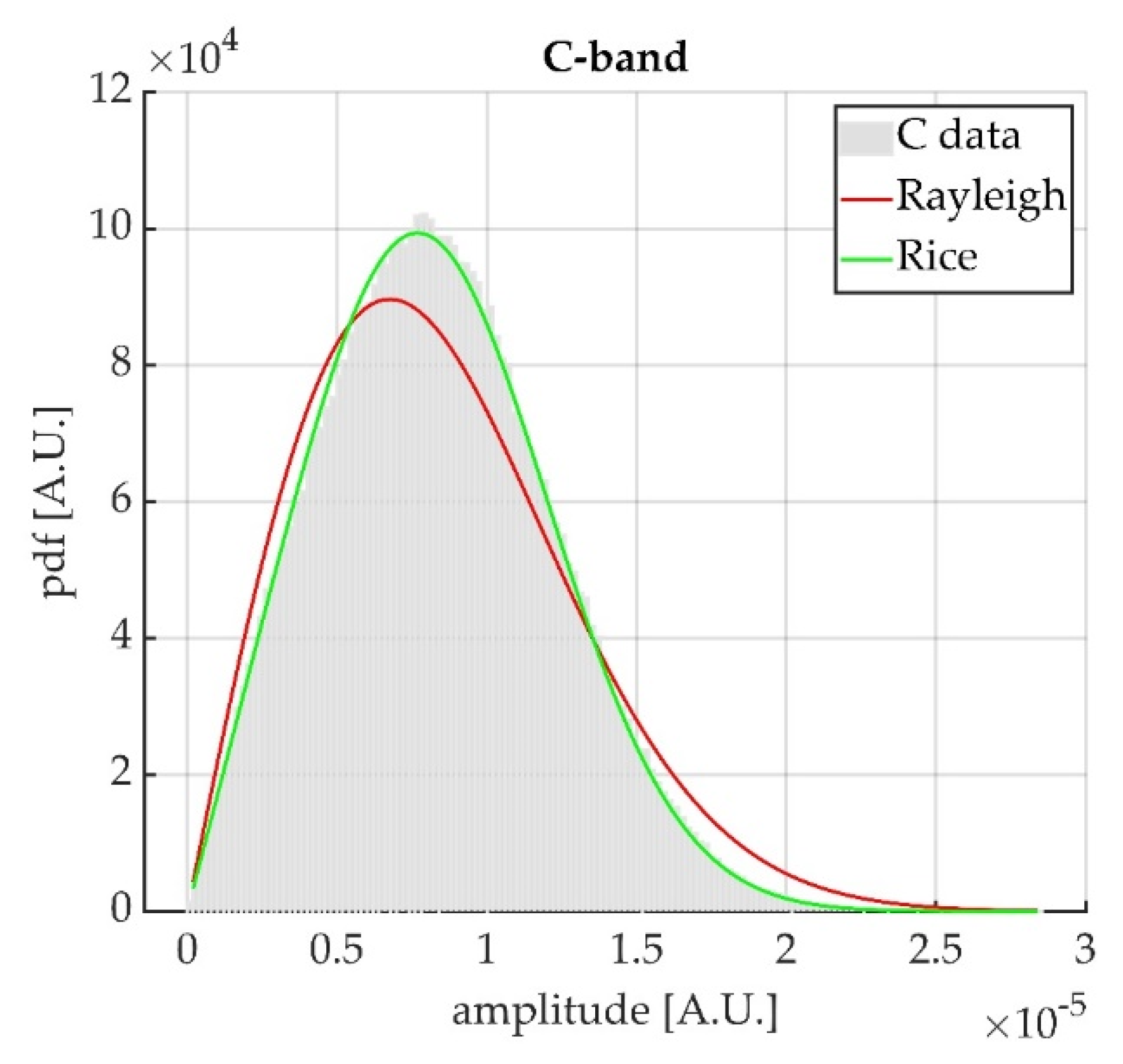
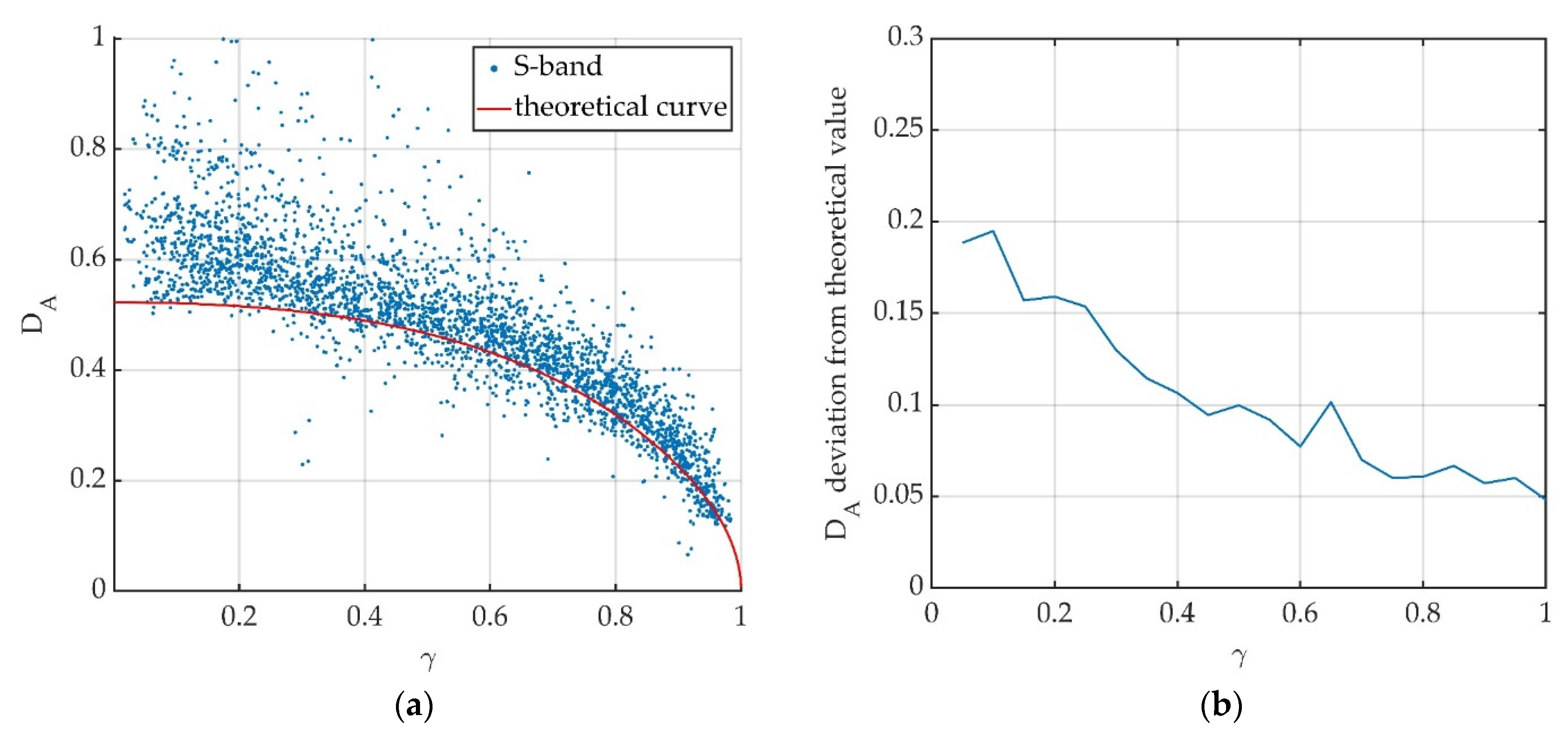
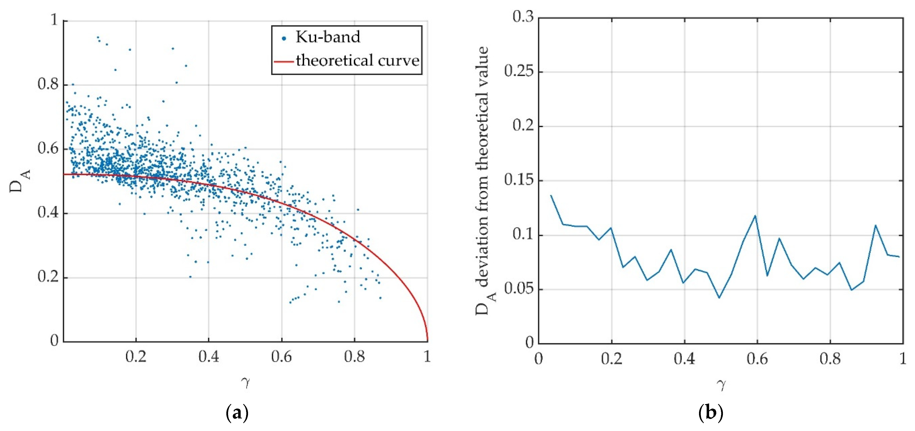
3.3. Measurements in Urban Scenario: Validation with Different Frequencies
4. Discussion
5. Conclusions
Author Contributions
Funding
Data Availability Statement
Acknowledgments
Conflicts of Interest
References
- Wang, Y.; Hong, W.; Zhang, Y.; Lin, Y.; Li, Y.; Bai, Z.; Zhang, Q.; Lv, S.; Liu, H.; Song, Y. Ground-Based Differential Interferometry SAR: A Review. IEEE Geosci. Remote Sens. Mag. 2020, 8, 43–70. [Google Scholar] [CrossRef]
- Zebker, H.; Villasenor, J. Decorrelation in interferometric radar echoes. IEEE Trans. Geosci. Remote Sens. 1992, 30, 950–959. [Google Scholar] [CrossRef] [Green Version]
- Lort, M.; Aguasca, A.; Lopez-Martinez, C.; Fabregas, X. Impact of Wind-Induced Scatterers Motion on GB-SAR Imaging. IEEE J. Sel. Top. Appl. Earth Obs. Remote Sens. 2018, 11, 3757–3768. [Google Scholar] [CrossRef] [Green Version]
- Monti-Guarnieri, A.; Manzoni, M.; Giudici, D.; Recchia, A.; Tebaldini, S. Vegetated Target Decorrelation in SAR and Interferometry: Models, Simulation, and Performance Evaluation. Remote Sens. 2020, 12, 2545. [Google Scholar] [CrossRef]
- Touzi, R.; Lopes, A.; Bruniquel, J.; Vachon, P.W. Coherence estimation for SAR imagery. IEEE Trans. Geosci. Remote Sens. 1999, 37, 135–149. [Google Scholar] [CrossRef] [Green Version]
- Crosetto, M.; Monserrat, O.; Cuevas-González, M.; Devanthéry, N.; Crippa, B. Persistent Scatterer Interferometry: A review. ISPRS J. Photogramm. Remote Sens. 2016, 115, 78–89. [Google Scholar] [CrossRef] [Green Version]
- Ferretti, A.; Prati, C.; Rocca, F. Permanent scatterers in SAR interferometry. IEEE Trans. Geosci. Remote Sens. 2001, 39, 8–20. [Google Scholar] [CrossRef]
- Goodman, J.W. Statistical Properties of Laser Speckle Patterns. In Laser Speckle and Related Phenomena; Dainty, J.C., Ed.; Springer: Berlin/Heidelberg, Germany, 1975; pp. 9–75. [Google Scholar] [CrossRef]
- Chitroub, S.; Houacine, A.; Sansal, B. Statistical characterisation and modelling of SAR images. Signal Process. 2002, 82, 69–92. [Google Scholar] [CrossRef]
- Gao, G. Statistical Modeling of SAR Images: A Survey. Sensors 2010, 10, 775–795. [Google Scholar] [CrossRef]
- Luzi, G.; Pieraccini, M.; Mecatti, D.; Noferini, L.; Guidi, G.; Moia, F.; Atzeni, C. Ground-based radar interferometry for landslides monitoring: Atmospheric and instrumental decorrelation sources on experimental data. IEEE Trans. Geosci. Remote Sens. 2004, 42, 2454–2466. [Google Scholar] [CrossRef]
- Wei, M.; Sandwell, D.T. Decorrelation of L-Band and C-Band Interferometry Over Vegetated Areas in California. IEEE Trans. Geosci. Remote Sens. 2010, 48, 2942–2952. [Google Scholar] [CrossRef]
- Iglesias, R.; Fabregas, X.; Aguasca, A.; Mallorqui, J.J.; Lopez-Martinez, C.; Gili, J.A.; Corominas, J. Atmospheric Phase Screen Compensation in Ground-Based SAR with a Multiple-Regression Model Over Mountainous Regions. IEEE Trans. Geosci. Remote Sens. 2013, 52, 2436–2449. [Google Scholar] [CrossRef]
- Iannini, L.; Guarnieri, A.M. Atmospheric Phase Screen in Ground-Based Radar: Statistics and Compensation. IEEE Geosci. Remote Sens. Lett. 2010, 8, 537–541. [Google Scholar] [CrossRef]
- Izumi, Y.; Nico, G.; Sato, M. Time-Series Clustering Methodology for Estimating Atmospheric Phase Screen in Ground-Based InSAR Data. IEEE Trans. Geosci. Remote Sens. 2021, 60, 1–9. [Google Scholar] [CrossRef]
- Hu, C.; Deng, Y.; Tian, W.; Zhao, Z. A Compensation Method for a Time–Space Variant Atmospheric Phase Applied to Time-Series GB-SAR Images. Remote Sens. 2019, 11, 2350. [Google Scholar] [CrossRef] [Green Version]
- Deng, Y.; Hu, C.; Tian, W.; Zhao, Z. A Grid Partition Method for Atmospheric Phase Compensation in GB-SAR. IEEE Trans. Geosci. Remote Sens. 2021, 60, 1–13. [Google Scholar] [CrossRef]
- Falabella, F.; Perrone, A.; Stabile, T.A.; Pepe, A. Atmospheric Phase Screen Compensation on Wrapped Ground-Based SAR Interferograms. IEEE Trans. Geosci. Remote Sens. 2021, 60, 1–15. [Google Scholar] [CrossRef]
- Rocca, F. Modeling Interferogram Stacks. IEEE Trans. Geosci. Remote Sens. 2007, 45, 3289–3299. [Google Scholar] [CrossRef]
- Tang, P.; Zhou, W.; Tian, B.; Chen, F.; Li, Z.; Li, G. Quantification of Temporal Decorrelation in X-, C-, and L-Band Interferometry for the Permafrost Region of the Qinghai–Tibet Plateau. IEEE Geosci. Remote Sens. Lett. 2017, 14, 2285–2289. [Google Scholar] [CrossRef]
- Morishita, Y.; Hanssen, R.F. Temporal Decorrelation in L-, C-, and X-band Satellite Radar Interferometry for Pasture on Drained Peat Soils. IEEE Trans. Geosci. Remote Sens. 2014, 53, 1096–1104. [Google Scholar] [CrossRef]
- Guarnieri, A.; Prati, C. SAR interferometry: A “Quick and dirty” coherence estimator for data browsing. IEEE Trans. Geosci. Remote Sens. 1997, 35, 660–669. [Google Scholar] [CrossRef] [Green Version]
- Lee, J.-S.; Cloude, S.; Papathanassiou, K.; Grunes, M.; Woodhouse, I. Speckle filtering and coherence estimation of polarimetric sar interferometry data for forest applications. IEEE Trans. Geosci. Remote Sens. 2003, 41, 2254–2263. [Google Scholar] [CrossRef]
- Carter, G.; Knapp, C.; Nuttall, A. Estimation of the magnitude-squared coherence function via overlapped fast Fourier transform processing. IEEE Trans. Audio Electroacoust. 1973, 21, 337–344. [Google Scholar] [CrossRef] [Green Version]
- Hinich, M.J.; Clay, C.S. The application of the discrete Fourier transform in the estimation of power spectra, coherence, and bispectra of geophysical data. Rev. Geophys. 1968, 6, 347–363. [Google Scholar] [CrossRef]
- Blasch, E.; Yang, C. FFT-based auto-correlation estimation (FACE) for extended radar pulse integration subject to large doppler change. In Proceedings of the 2012 11th International Conference on Information Science, Signal Processing and their Applications (ISSPA), Montreal, QC, Canada, 2–5 July 2012; pp. 1153–1158. [Google Scholar] [CrossRef]
- Holzner, J. Analysis and statistical characterization of interferometric SAR signals based on the power spectral density function. IEEE Trans. Geosci. Remote Sens. 2004, 42, 1116–1121. [Google Scholar] [CrossRef]
- Qiu, Z.; Ma, Y.; Guo, X. Atmospheric phase screen correction in ground-based SAR with PS technique. SpringerPlus 2016, 5, 1594. [Google Scholar] [CrossRef] [Green Version]
- Noferini, L.; Pieraccini, M.; Mecatti, D.; Luzi, G.; Atzeni, C.; Tamburini, A.; Broccolato, M. Permanent scatterers analysis for atmospheric correction in ground-based SAR interferometry. IEEE Trans. Geosci. Remote Sens. 2005, 43, 1459–1471. [Google Scholar] [CrossRef]
- Tough, R.J.A.; Blacknell, D.; Quegan, S. A statistical description of polarimetric and interferometric synthetic aperture radar data. Proc. R. Soc. Lond. Ser. A Math. Phys. Sci. 1995, 449, 567–589. [Google Scholar] [CrossRef]
- Donati, S.; Martini, G. Speckle-pattern intensity and phase: Second-order conditional statistics. J. Opt. Soc. Am. 1979, 69, 1690–1694. [Google Scholar] [CrossRef]
- Bamler, R.; Just, D. Phase statistics and decorrelation in SAR interferograms. In Proceedings of the IGARSS’93—IEEE International Geoscience and Remote Sensing Symposium, Tokyo, Japan, 18–21 August 2002. [Google Scholar] [CrossRef]
- Bamler, R.; Hartl, P. Synthetic aperture radar interferometry. Inverse Probl. 1998, 14, R1–R54. [Google Scholar] [CrossRef]
- Pieraccini, M.; Miccinesi, L. ArcSAR: Theory, Simulations, and Experimental Verification. IEEE Trans. Microw. Theory Tech. 2016, 65, 293–301. [Google Scholar] [CrossRef]
- Di Pasquale, A.; Nico, G.; Pitullo, A.; Prezioso, G. Monitoring Strategies of Earth Dams by Ground-Based Radar Interferometry: How to Extract Useful Information for Seismic Risk Assessment. Sensors 2018, 18, 244. [Google Scholar] [CrossRef] [PubMed] [Green Version]


Publisher’s Note: MDPI stays neutral with regard to jurisdictional claims in published maps and institutional affiliations. |
© 2022 by the authors. Licensee MDPI, Basel, Switzerland. This article is an open access article distributed under the terms and conditions of the Creative Commons Attribution (CC BY) license (https://creativecommons.org/licenses/by/4.0/).
Share and Cite
Beni, A.; Miccinesi, L.; Michelini, A.; Pieraccini, M. Temporal Coherence Estimators for GBSAR. Remote Sens. 2022, 14, 3039. https://doi.org/10.3390/rs14133039
Beni A, Miccinesi L, Michelini A, Pieraccini M. Temporal Coherence Estimators for GBSAR. Remote Sensing. 2022; 14(13):3039. https://doi.org/10.3390/rs14133039
Chicago/Turabian StyleBeni, Alessandra, Lapo Miccinesi, Alberto Michelini, and Massimiliano Pieraccini. 2022. "Temporal Coherence Estimators for GBSAR" Remote Sensing 14, no. 13: 3039. https://doi.org/10.3390/rs14133039
APA StyleBeni, A., Miccinesi, L., Michelini, A., & Pieraccini, M. (2022). Temporal Coherence Estimators for GBSAR. Remote Sensing, 14(13), 3039. https://doi.org/10.3390/rs14133039