Abstract
The observation of taking-off and landing behaviors of migratory insects is important for pest early monitoring and forecasting. Entomological radar, which can measure the ascent or descent rates remotely, has been proved to be the most effective way to observe the above behaviors. For the current entomological radars, the highest range resolution of 7.5 m and smallest blind range of 150 m make it difficult to distinguish individual insects in a swarm and observe the migratory behaviors at low altitudes. In this paper, based on the outfield data acquired from a high-resolution radar of 0.2 m, the spatial spacing distribution of migratory insects is presented for the first time and waveform design requirements are analyzed, proving the necessity of a higher resolution. Secondly, for the high-resolution and low blind range observation of insects, the stepped frequency train of LFM pulses (also called frequency-jumped burst, FJB) waveform is discussed as the optimal choice. In order to resolve the high grating-lobe problem in the FJB waveform with the low blind range, the precise spectrum model and its approximation of the LFM subpulse are first derived in detail. Then, according to the obtained spectrum characteristics, the high-resolution and low blind range FJB waveform design methods based on spectrum fluctuation period and Fresnel integral windowing are proposed to reduce the grating-lobe number to more than 50% and suppress the highest grating lobe level by at least 4 dB. Finally, based on the high-resolution and low blind range VLR adopting the proposed waveform, several typical taking-off and landing behavior observation results are presented, which proves that, in their migratory pattern, insects usually take off around sunset.
1. Introduction
Billions of insects migrate within or between the continents every year [1]. Many of them having strong migration ability may induce pest outbreaks and cause significant damage to the crops [2]. During 2016~2020, the well-known maize pest Spodoptera frugiperda migrated from Nigeria to most parts of Africa, Asia, and Oceanica without human help. Because of the high-water content of the insect’s body, the radar cross-section (RCS) of insects has been proven to be approximated as a spherical water droplet of the same mass, and has the potential to be detected by radar [3,4,5,6,7,8]. To realize the pests’ early monitoring and forecasting, entomological radar was specially built and has been the most effective means to observe the insect behavior without affecting their migration and helped to discover several migration phenomena, such as layering and common orientation [9,10,11]. In more than half a century of development, various entomological radars have been developed, including scanning radar, airborne radar, harmonic radar, and vertical looking radar (VLR) [12,13,14]. VLR, which employs a vertically pointing, nutating beam with a rotating linear polarization, can measure migratory insects’ behavioral and biological parameters remotely and automatically through complex signal processing [15,16]. For insects’ monitoring and forecasting based on VLRs, it is necessary to know when insects reach or leave an area so as to detect the pest invasion in advance, and to carry out corresponding pest control promptly before they reproduce on a large scale. Therefore, it is important to observe the taking-off and landing behaviors of the migratory insects, in which the ascent or descent rate is the key parameter to be measured.
The ascent or descent rate of migratory insects is measured by the linear or parabolic fitting of insect flight tracks in current VLRs [17,18]. Hence, its precision depends on the effective observation of the flight track, which includes the high-resolution measurement of the insects’ height and the effective detection of the tiny insects from the background noise. For the detection of insects, several methods have been proposed and proven their robustness in operation [19,20,21,22,23,24]. For the high-resolution measurement of the insects, the current VLRs are all non-coherent and emit unmodulated pulses with the pulse width of 0.05 μs, 0.08 μs, or 0.1 μs, corresponding to the range resolution of 7.5, 12, or 15 m respectively [18,22,25]. When the track spacings of insects are lower than the range resolution, VLRs may be unable to distinguish the individual insects, leading to interference from multiple-target flight tracks. However, there is little information about the migratory insect spacings measured in a higher-resolution way. Hence, it is unclear whether the range resolutions of current VLRs can meet the observation requirements of individuals in migratory swarms. In addition, the taking-off and landing behaviors usually occur in low altitudes. Table 1 presents the migratory heights of several key agricultural pests, and the lower limits are usually below 100 m. The 150 or 175 m blind range of current VLRs makes it difficult to observe the flight behavior of low-altitude insects [23,26]. Therefore, to observe the taking-off and landing behaviors of the migratory insects, it is necessary to realize the high-resolution and low blind observation of VLRs.

Table 1.
Migration height of typical insects.
Adopting the high range resolution waveform is the main method to achieve high-resolution observation of targets on radar. Radar’s range resolution is inversely proportional to the bandwidth; thus, to achieve the high-resolution measurement, a large bandwidth is needed. The wideband waveforms consist mainly of three categories: the ultra-wideband (UWB) spike pulse, linear frequency modulation (LFM) pulse, and the stepped frequency train of LFM pulses (also called frequency-jumped burst, FJB) [27]. The form of the UWB spike pulse is the same as that of unmodulated pulses used in current VLRs, but the pulse width is reduced to the nanosecond level. The corresponding range resolution can be better than 1 m. However, the extremely short pulse width of the UWB waveform leads to the low average power of the radar transmitter, making it only suitable for the detection of close-in targets. LFM pulse modulates the instantaneous frequency of the signal within the pulse width to obtain the wide bandwidth and realizes the high range resolution by pulse compression technology. It can obtain the wideband while ensuring the transmitting power and has been widely used in the high-resolution measurement of traditional radar targets, such as aircraft and missiles. However, because the insects’ taking-off and landing behavior observation requires a low blind range, the pulse width of the LFM signal should be set to less than 0.6 μs. Modulating a wideband signal in such a small pulse width will increase the cost and complexity of hardware implementation markedly, which is adverse to the extension and application of the entomological radar. FJB waveform is the variant of the traditional wideband LFM pulse. It transmits a series of narrow-band LFM pulses with a stepped center frequency and obtains the synthesized wideband spectrum through signal processing. Because the actual instantaneous bandwidth is much smaller than the synthesized total bandwidth, it greatly reduces the complexity of the high-resolution system. Therefore, the FJB waveform is an optimal choice for the high resolution and low blind range observation of migratory insects. However, the inherent recurrent grating lobes in the synthesized high range resolution profile (HRRP) may cause the missed detection of the weak targets when strong and weak targets appear simultaneously. Particularly, the small pulse width of the narrow-band LFM pulses required for low blind range observation leads to a further deterioration in the grating-lobe problem.
There are two types of methods to suppress the grating lobes of the FJB waveform, namely, waveform design methods and signal processing methods. The signal processing methods do not change the emitted waveform but adopt the windowing or magnitude/phase error compensation technologies to restructure the synthesized wideband spectrum based on the received echoes so as to suppress the grating lobe in the small pulse width [28,29,30,31,32]. However, the former windowing method leads to the reduction in range resolution, loss of signal to noise ratio (SNR), or the missing of weak targets, which reduces the detection performance of radar for tiny insects. In the latter compensation methods, the magnitude/phase error needs to be estimated frequently and compensated for HRRP, which is time-consuming and laborious. Moreover, it compensates for the inherent amplitude and phase fluctuations of the waveform and system errors simultaneously, which changes the scattering characteristics of the targets measured at different times and affects the body parameter measurement based on the insects’ RCS. In addition to signal processing methods, several waveform design methods have been also proposed. Ref. [33] derived the autocorrelation function (ACF) of the FJB waveform, and presented the relationships among the stepped frequency, pulse width, and bandwidth for nullifying the several even all grating lobes directly on some parameter combinations. Based on the ACF, a generalized method, which suppresses all the grating lobe levels to the desired threshold, was further proposed [34,35,36,37]. Several optimization methods were also proposed to obtain the optimized parameter combinations [38,39]. Under the above waveform design results, the grating lobes in small pulse width/blind range conditions can be suppressed. However, the ACF represents the matching filtering results of the waveform at different delays. The frequency-domain stepped-frequency processing (FD-SFP), commonly used to synthesize the HRRP, includes the additional nonlinear operation as shown in Figure 1 [28]. This results in a significant difference between the obtained HRRP and matched filter output, and the conclusions based on ACF are not applicable [40,41]. Therefore, it is necessary to study the grating-lobe suppression in the HRRP based on the FD-SFP, especially under the small pulse width.

Figure 1.
Flowchart of frequency-domain stepped-frequency processing method.
In this paper, to solve the low range resolution and high blind range problems of current VLRs in the migratory insects’ taking-off and landing behavior observation, the high range resolution and low blind range FJB waveform design methods are proposed. First, based on 254,000 flight tracks acquired from a high-resolution radar of 0.2 m in the migration season, the spatial spacing distribution of migratory insects are analyzed for the first time. The results show that the tracks with spacings below the highest range resolution (7.5 m) of current VLRs account for 11.0%, which proves that the range resolution of VLR needs to be further improved. Secondly, considering the cost and complexity of the hardware implementation, the FJB waveform is found to be the optimal choice for the high-resolution and low blind range observation of insects. However, the inherently periodic grating-lobe problem of the FJB waveform becomes serious and cannot be ignored when the blind range is low. To resolve the high grating-lobe problems under the low blind range, the spectrum model and its precise approximation of the LFM subpulse is first derived in detail. Then, the high-resolution and low blind range waveform design methods based on spectrum fluctuation period and Fresnel integral windowing are proposed to reduce the grating-lobe number to 50% and suppress the grating-lobe level by more than 4 dB. Finally, based on the high-resolution and low blind range VLR adopting the proposed waveform, the taking-off and landing behavior observation results are presented and the migratory behavior patterns are analyzed.
The remainder of this article is organized as follows. In Section 2, based on the field data acquired from a high-resolution VLR of 0.2 m, the spacings distribution of migratory insects and the radar waveform design requirement for the taking-off and landing behavior observation are analyzed. In Section 3, the spectrum model of the small time-bandwidth product FJB waveform is built based on the Fresnel integral and its high-precision approximations. According to the spectrum fluctuation characteristics, the high-resolution and low blind range waveform design methods based on the spectrum fluctuation period and Fresnel integral windowing are presented in detail. In Section 4, the performance of the proposed waveform method is evaluated using simulation analysis and experimental data. In Section 5, the proposed waveform is applied to the high-resolution and low blind range coherent VLRs. The ascent and descent rates of migratory insects are measured precisely, and several taking-off and landing behavior observation results are presented and analyzed. In Section 6 and Section 7, the discussion and conclusions of this work are drawn.
2. Waveform Requirement Analysis for Taking-Off/Landing Behavior Observation
Analyzing the observation requirements of take-off and landing behaviors is essential for the parameter design of radar waveforms. Specifically, the blind range and resolution are determined by the targets’ flight heights and spatial spacings. The blind range is the lower limit of the radar detection range and is proportional to the pulse width, whereas the range resolution represents the radar’s ability to distinguish close-in targets. Based on the results from current entomological radars, the flight heights of several insects have been obtained, and some typical results are given in Table 1. However, there is little information about the spatial spacings of the migratory insects due to the lack of high-resolution remote observation ways. It is unclear whether the highest range resolution (7.5 m) of current VLRs can realize the effective measurement of individual insects in the swarm. Therefore, in this section, based on a high-resolution coherent VLR, the spatial spacings of migratory insects are analyzed, which provides a reference for the design of range resolution of the entomological radar.
2.1. Data Description
To analyze the spatial spacings of migratory insects, a high-resolution coherent VLR was used to collect a large amount of data in May 2020. The radar has been placed in Lancang (22.506995°N, 99.887471°E), Yunnan Province, China, since 2019, as shown in Figure 2. It was initially set to operate from 7:00 p.m. to 7:00 a.m. the next day and was upgraded to work all day in 2020. The main parameters of the high-resolution coherent VLR are listed in Table 2. The radar is operated at the Ku band and adapts a parabolic antenna with a diameter of 1 m to emit the FJB waveform. A transceiver with a peak power of 30 w is used to produce radio frequency pulses and transform received echoes into baseband.
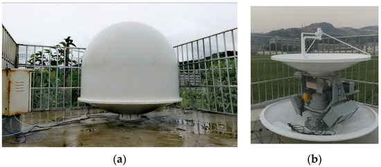
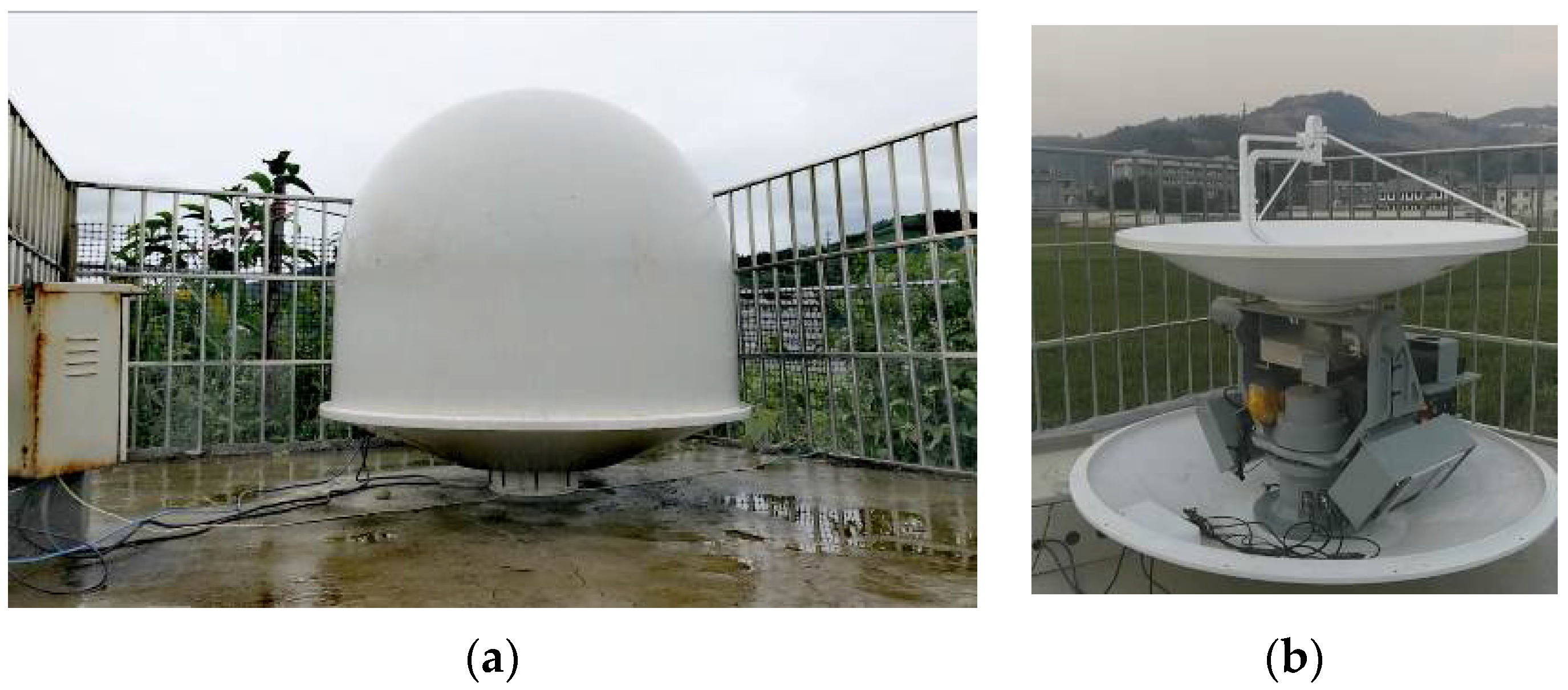
Figure 2.
High-resolution coherent VLR at Lancang, Yunnan Province, China: (a) photo in operation mode; (b) internal structure.
Table 2.
Main parameters of the high-resolution coherent VLR.
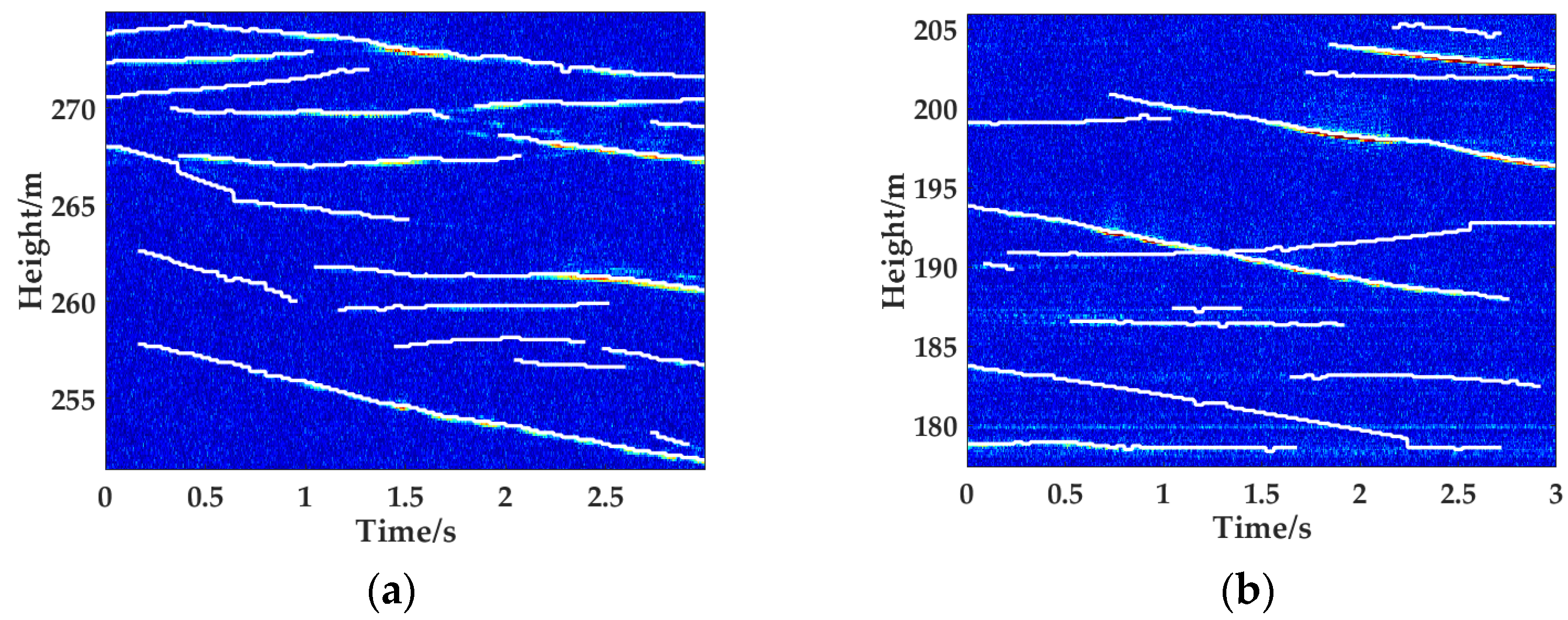
The signal processing flow from the baseband echoes to the insects’ tracks is shown in Figure 3 [24]. First, for the received baseband echoes, the HRRPs are obtained by FD-SFP [29,41,42]. The stepped frequency and subpulse number are set as 20 MHz and 40, and the range resolution is 0.1875 m, which is much higher than current VLRs. To facilitate digital signal processing, the points in the synthesized wideband spectrum are increased to the integer power of 2 by zero-padding, hence reducing the range interval between sampling points to 0.1172 m. Two typical HRRPs within an operation cycle of 3 s are presented in Figure 4a,b, respectively. Second, for the migratory insect detection in the high-resolution coherent VLR, the typical algorithm combinations composed of the pulse-Doppler (PD) integration and constant false alarm rate (CFAR) detector are adopted [43]. PD integration with a coherent integration interval (CPI) of 20 ms is used to improve the detection SNR of tiny insects. The CFAR detector is followed to find the target points (locations) in each HRRP with the false alarm rate of 1 × 10⁻⁶. Finally, the target tracks of the migratory insects are obtained by the nearest neighbor association of the detected insect locations between the adjacent CPIs. The detected tracks of the HRRPs in Figure 4a,b are presented as white lines. Moreover, to improve the operation efficiency of the CFAR detector, the CFAR threshold decision is not applied to all the samples but only to the local power maximums within the adjacent five samples. Therefore, the minimum spacing between the detected insects is 0.5859 m.

Figure 3.
Signal processing of the high-resolution coherent VLR.

Figure 4.
(a,b) Two typical HRRPs and the detected flight tracks by the high-resolution coherent VLR.
Next, based on 254,000 temporally overlapping flight tracks with overlapping in time detected by the high-resolution coherent VLR in Lancang, Yunnan Province, China, the spatial spacings of the migratory insects are analyzed.
2.2. Requirement Analysis of Waveform Design
In order to obtain the spatial spacings of the migratory insects, the flight tracks observed by the high-resolution coherent VLR in the migration season of 2020 are chosen as the samples for analysis. There is a total of 254,000 flight tracks overlapping in time. The spatial spacing of any two insects is defined as the minimum of height absolute difference between the flight tracks, which can be expressed as follow
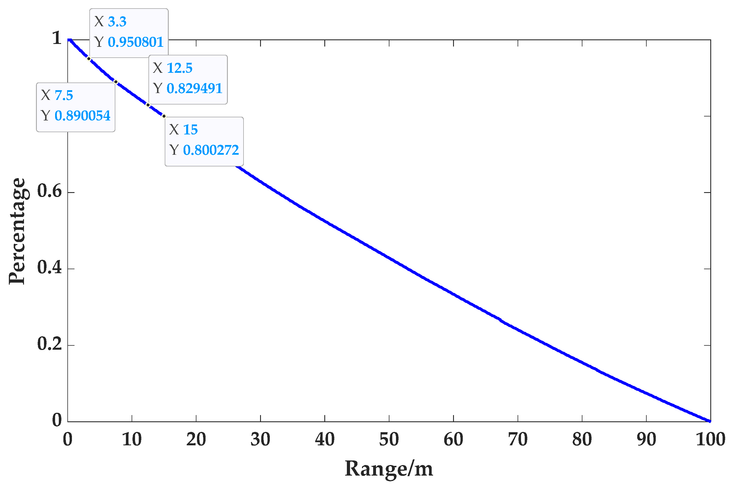
where and are the heights of two temporally overlapping flight tracks, is the overlapped time. Considering multiple insects may be detected by the VLR simultaneously, the number of the calculated track spacings will far exceed that of tracks. For simplicity, only the spacings less than 100 m were analyzed, and 308,605 spatial spacings meet the above conditions.
Finally, the percentage of insect spatial spacing greater than a certain range is shown in Figure 5. It can be seen that the spacing that is greater than 3.3 m accounts for 95%, which means that the range resolution of VLRs should be better than 3.3 m to distinguish more than 95% of close individual insects. Moreover, the percentages of the spacings in the ranges 0~7.5 m, 7.5~12 m, and 12~15 m are 11.0%, 5.5%, and 3.5%, respectively. Because the range resolutions of current VLRs are mainly 7.5, 12, and 15 m, of which the range resolutions of 7.5 and 15 m are the most widely used, about 20% of track spacings in total are lower than the resolution of 15 m. About 11.0% exceed the highest resolution of all current VLRs. Therefore, it can be proved that a range resolution higher than 7.5 m is needed for the effective observation of migratory insects.
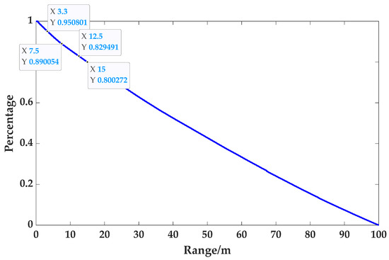
Figure 5.
Percentages of insects’ spacings greater than a certain value.
In summary, the spacing analysis of migratory insects proves that a higher range resolution for VLRs is needed to observe insect behaviors. Moreover, as listed in Table 1, the minimum migratory heights of the several typical insects are below 100 m. At the same time, the taking-off and landing behaviors of the migratory insects usually occur in low-altitude areas; hence, a low blind range waveform is also required.
3. High-Resolution and Low Blind Range Waveform Design Method
As discussed in Section 2, the high-resolution and low blind range waveform is required for the taking-off and landing behavior observation of migratory insects. Considering the implementation cost and complexity, the FJB waveform is the optimal choice. However, the inherent recurrent grating lobes of the FJB waveform cannot be ignored when the pulse width or the time-bandwidth product is small, which may raise the background noise and even submerge the weak target. Hence, it is necessary to suppress the grating lobes of the FJB waveform.
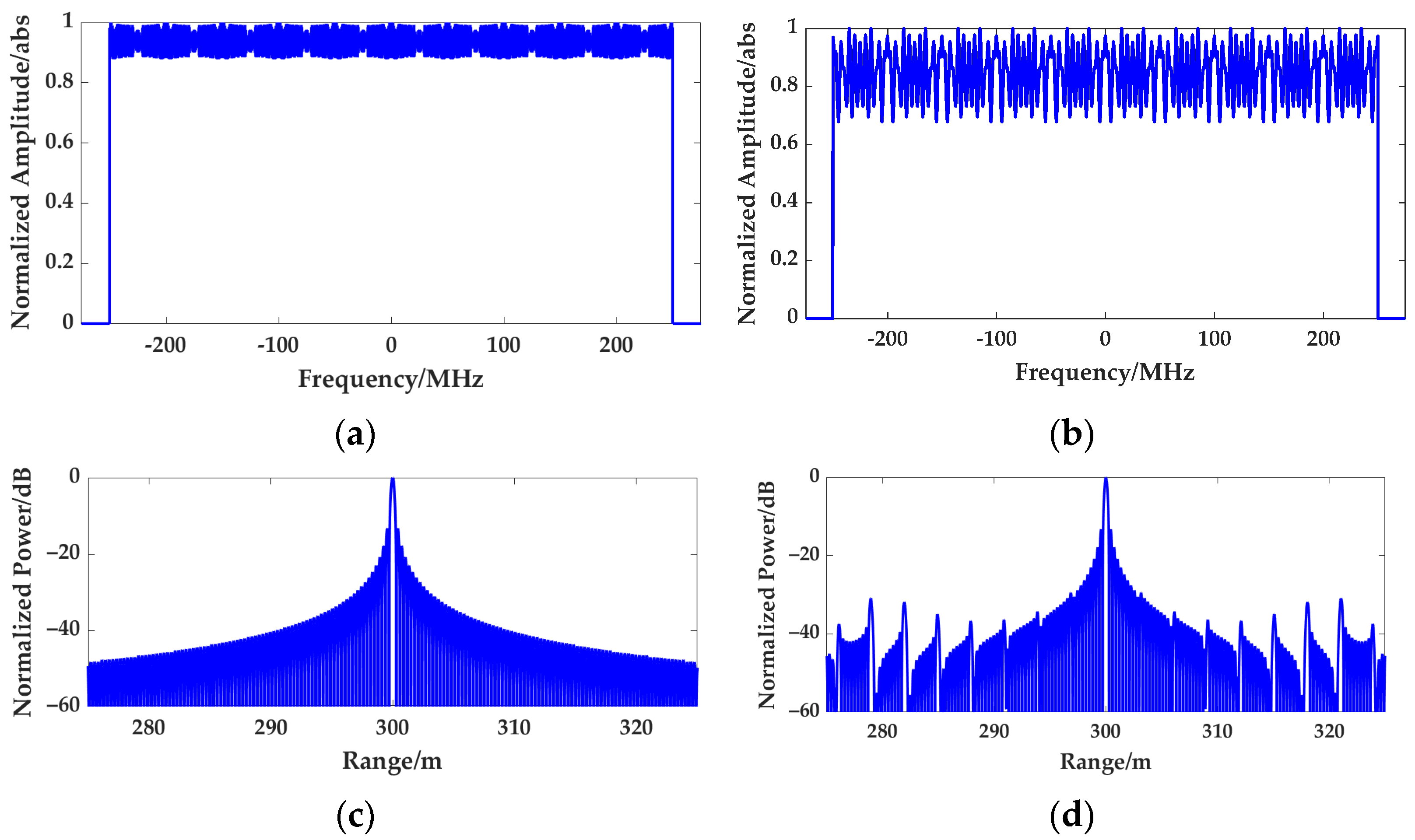
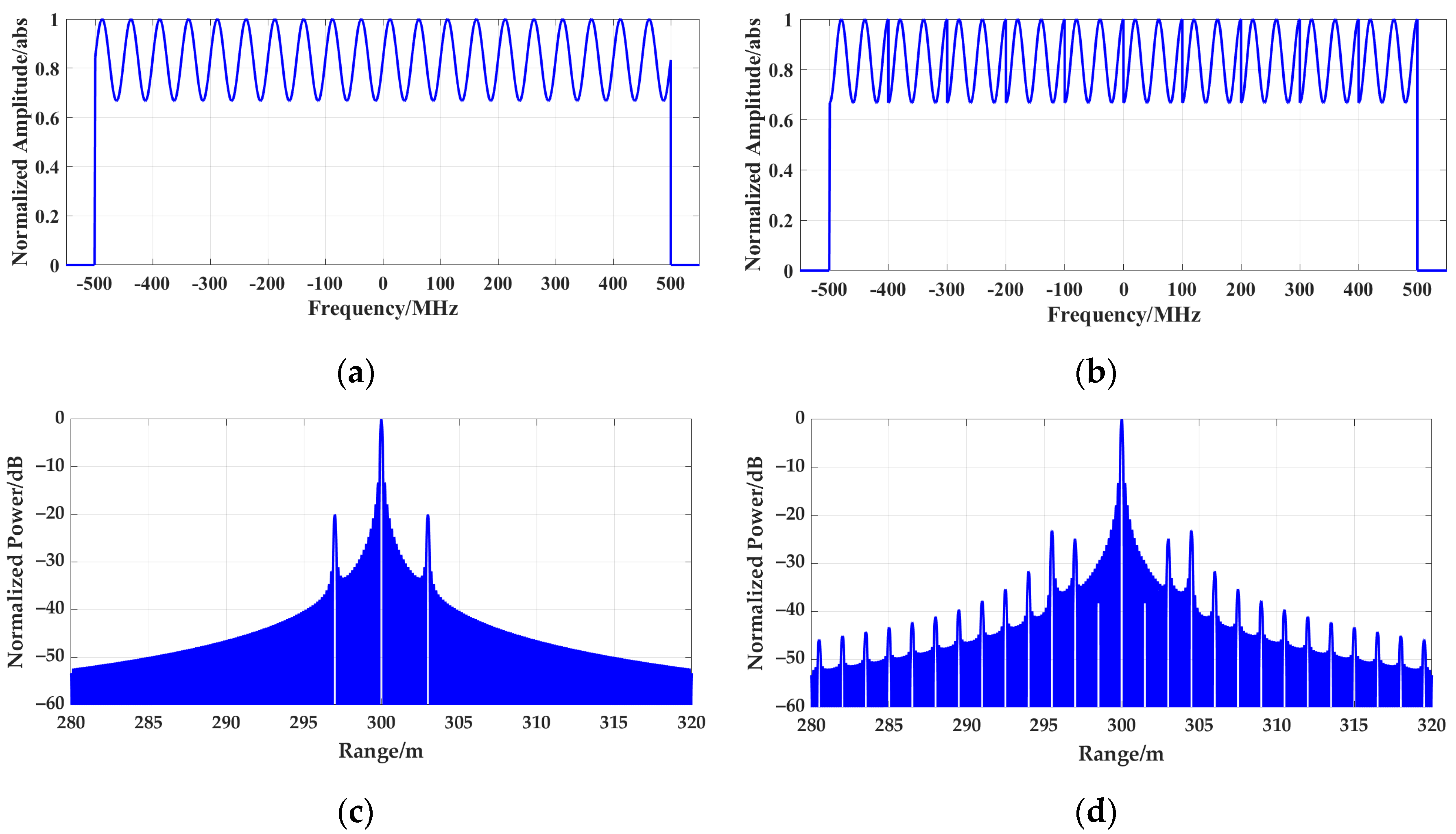
For the FJB waveform with the large time-bandwidth product LFM subpulse, the synthesized wideband spectrum and HRRP are shown in Figure 6a,c. Its spectrum amplitude is flat, and there are no grating lobes in the HRRP. However, the synthesized results under small time-bandwidth product condition are presented in Figure 6b,d, which show the spectrum with greater fluctuation and the HRRP with higher grating lobes. Therefore, it can be concluded that the grating lobes in HRRPs are mainly caused by the strong amplitude fluctuation in the spectrum. Because the synthesized spectrum is the splicing of the narrow-band LFM match-filtered spectrum, the level of grating lobes in HRRP mainly depends on the spectrum of the small time-bandwidth product LFM subpulse. Therefore, it is necessary to study the spectrum amplitude characteristics of the small time-bandwidth product LFM pulse.

Figure 6.
Synthesized results under large and small time-bandwidth product conditions: (a,c) synthesized wideband spectrum and HRRP based on the LFM subpulse with the time-bandwidth product of 500; (b,d) synthesized wideband spectrum and HRRP based on the LFM subpulse with the time-bandwidth product of 50.
To solve the grating-lobe problem in the small time-bandwidth product, in this section, the spectrum model and its approximate expression of the narrow-band LFM subpulse are first derived in detail. On the basis of the spectrum amplitude characteristics, the FJB waveform design methods based on spectrum fluctuation period and Fresnel integral windowing are proposed to realize the high-resolution, low blind range, and low grating-lobe observation.
3.1. Spectrum Modeling of Small Time-Bandwidth Product LFM Subpulse
The expression of baseband LFM pulse with unit energy is
Fourier transform of (2) yields its spectrum as
where , . is Fresnel integral and can be expanded as
where and [44]. Because the frequency , the range of and are and respectively. To facilitate subsequent analysis, and should be transformed to the same intervals. Considering is an odd function, can be modified as , where and we have
Because the amplitude of the match-filtered spectrum is the square of the LFM spectrum amplitude, by substituting described in (9) by (10), can be expressed as follows:
Because and are difficult to simplify further, there is little research based on the spectral characteristics of the LFM pulse. However, several precise approximation formulas of Fresnel integral have been proposed for reference [45]. One precise approximation formula can be written as
where
By substituting and described in (6) by (7), at the same time considering , and the product among , , , are relatively small to negligible, the approximation formula of the match-filtered spectrum can be simplified as
Further simplify and to
Finally, the approximate spectrum model of can be simplified as
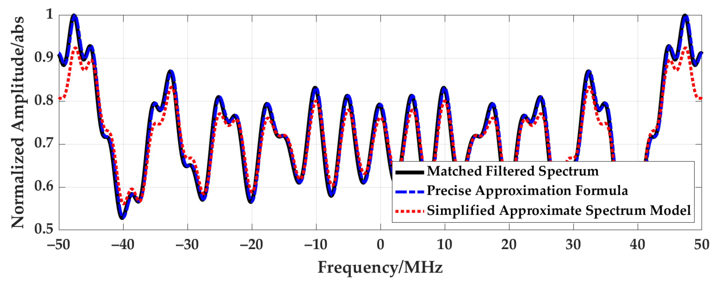
To verify (11), taking the LFM pulse with a pulse width of 0.4 μs and bandwidth of 125 MHz as an example, the match-filtered spectrum, the precise approximation formula in (6), and the simplified approximate spectrum model proposed in this section are simulated, and the results are illustrated in Figure 7. It can be seen that the precise approximation formula is the same as the match-filtered spectrum. The fluctuation characteristic of the simplified approximate spectrum model is basically consistent with that of the former, and only the amplitude at some frequency decreases slightly, which proves that the simplified approximate spectrum model can be used to describe the spectrum fluctuation characteristic of the small time-bandwidth product LFM pulse.

Figure 7.
Simulation result of the match-filtered spectrum and the corresponding numerical results based on precise approximation formula and simplified approximate formula.
Based on the above analysis, the amplitude fluctuation of the synthesized spectrum is the main theoretical reason for the grating-lobe problem. It can be expanded into the sum of several different sinusoidal terms. The amplitude and period of each sinusoidal term respectively correspond to a pair of grating lobes’ levels and positions. In the next section, based on the amplitude and period of the derived spectrum model, the low blind range and low grating-lobe waveform design methods for the small time-bandwidth product FJB waveform are proposed, which are carried out from two aspects: the reductions of the grating-lobe number and levels.
3.2. Grating-Lobe Number Reduction Method Based on Spectrum Fluctuation Period
As shown in Figure 7, the match-filtered spectrum of the small time-bandwidth product LFM subpulse presents a periodic sinusoidal-like fluctuation along both sides of zero frequency. Because the synthesized spectrum is the splicing of the narrow-band LFM match-filtered spectrum, its sinusoidal expansion results are greatly affected by the continuity of the synthesized spectrum. When the amplitude of the synthesized spectrum is a continuous function similar to the sine curve, there are only 1~2 sinusoidal terms with high amplitude in all the sinusoidal expansion results, corresponding to only 1 to 2 pairs of high grating lobes in HRRP as shown in Figure 8a,c. Otherwise, when the amplitude of the synthesized spectrum is discontinuous, its sinusoidal expansion results will contain several sinusoidal terms whose amplitudes are slightly smaller amplitude than those of sinusoidal terms in the continuous synthesized spectrum, as shown in Figure 8b,d. This leads to several grating lobes in HRRP with slightly lower levels but a much larger number. Therefore, to reduce the number of grating lobes, making the synthesized spectrum as continuous as possible is necessary.
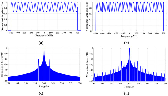
Figure 8.
Amplitude of synthesized wideband spectrum and corresponding HRRPs: (a) synthesized wideband spectrum with the continuous sinusoidal amplitude; (b) synthesized wideband spectrum with the discontinuous sinusoidal amplitude; (c) HRRP with the continuous sinusoidal amplitude spectrum; (d) HRRP with the discontinuous sinusoidal amplitude spectrum.
When the stepped frequency is the integer multiple of the spectrum fluctuation period, the derivative at the splicing point between the subpulse spectrum is 0, making the synthesized spectrum continuous. In order to obtain the spectrum fluctuation period of the small time-bandwidth product LFM subpulse, the derivative of the simplified approximate spectrum model in (11) is solved first, and then find the positions whose derivatives are zero, that is, the positions of the extreme points.
First, the four product terms in (11) are rewritten as
where .
Then, the derivative of can be expressed as
where the derivative of , , , are
Since a ≫ b, when f is small, to make , it requires that
Finally, we have the positions of the extreme points as
This shows that the spectrum fluctuation period is the inverse of the frequency difference between adjacent peak values, i.e., .
Therefore, we conclude that for the FJB waveform with the small time-bandwidth product LFM subpulse, the stepped frequency should be the integer multiple of to maintain the continuity of the synthesized spectrum. Thus, the amplitude of the synthesized spectrum can be approximated as a sinusoidal function with a fluctuation period of and can be expressed as
where A is the normalized fluctuation amplitude of the synthesized wideband spectrum.
By performing the inverse Fourier transform of (17), the corresponding HRRP is obtained as
This means that when the stepped frequency is limited and selected as the integer multiple of , there is only one pair of symmetrical grating lobes with the normalized grating-lobe level of and the delay of in HRRP, thus effectively reducing the grating-lobe number.
3.3. Grating-Lobe Level Suppression Method Based on Fresnel Integral Windowing
In Section 3.2, the number of grating lobes is effectively reduced by setting the stepped frequency as the integer multiple of the spectrum fluctuation period. However, this also leads to an increase in the grating-lobe levels. Based on (18), the grating-lobe level of the FJB waveform depends on the normalized fluctuation amplitude. Therefore, in this section, a time-domain windowing method is proposed to suppress the spectrum fluctuation amplitude without changing the fluctuation characteristic, which reduces the numbers and levels of the grating lobes simultaneously by combining with the method described in Section 3.2.
First, considering the limit case of suppressing the frequency spectrum of the small time-bandwidth product LFM pulse into a rectangular window, the corresponding normalized spectrum can be expressed as
Then, by performing the inverse Fourier transform, the time-domain expression is obtained as
where the expression of and are
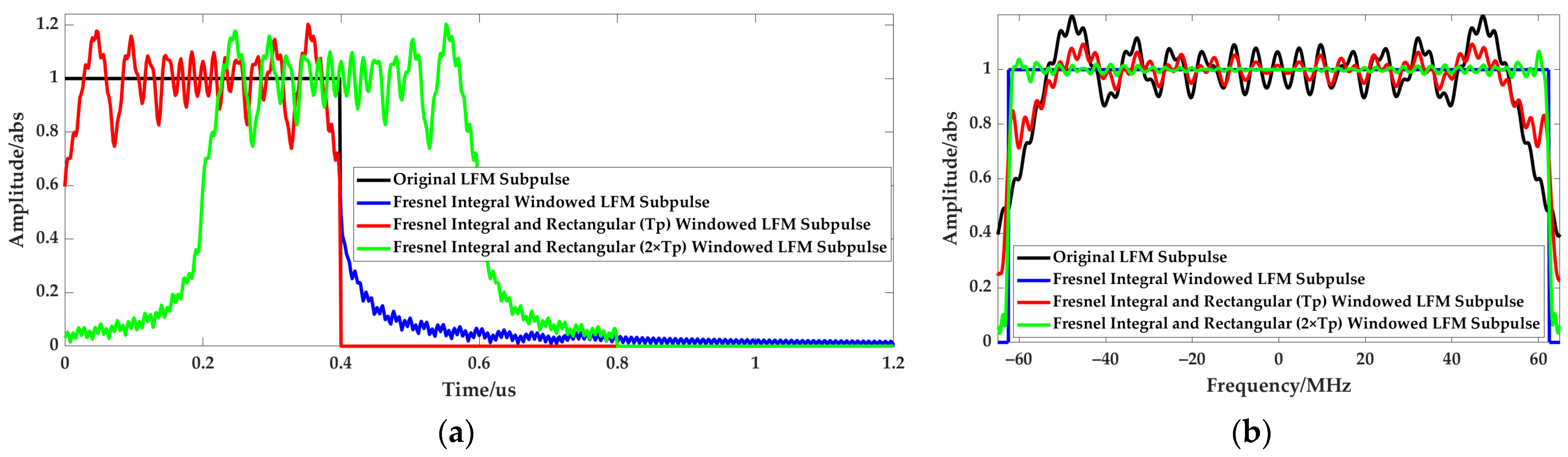
Therefore, the rectangular spectrum can be obtained by Fresnel integral windowing to the original LFM pulse, as shown in the blue line of Figure 9a. However, the Fresnel integral window is not a rectangular pulse in the time domain but slowly decreases along both sides of the original rectangular pulse. This will increase the transmit signal width and makes the VLRs difficult to observe the taking-off and landing behaviors at low altitude. An additional rectangular window is considered to be superposed to limit the width of the Fresnel integral windowed pulse. The obtained spectrum will present the fluctuation similar to that of the original LFM pulse due to the rapid rise and fall in the time domain. This operation partially offsets the effect of Fresnel integral windowing. However, the spectrum fluctuation is still significantly suppressed compared to that of the original LFM pulse, as shown in the red line in Figure 9b. With the increase in the additional rectangular window width, the amplitude of the spectrum fluctuation gradually decreases, and the spectrum can converge to the rectangular shape, as shown in the green line in Figure 9b. Therefore, it is necessary to determine the width of the additional rectangular window.
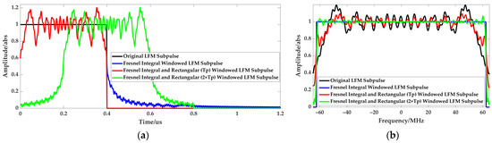
Figure 9.
(a) Time-domain waveform of original LFM subpulse and its Fresnel integral windowed subpulse; (b) corresponding spectrums of the subpulse in (a).
Moreover, as shown in Figure 9b, the spectrum amplitude of the Fresnel integral and rectangular windowed LFM subpulse presents a sinusoidal shape with a period of . Hence, the spectrum in (19) can be rewritten as
where A′ is the normalized fluctuation amplitude of the LFM pulse spectrum.
Based on the inverse Fourier transform of is , we have the time domain expression of as follows:
Because the time range of is limited to by the additional rectangular window, the range of in (23) is . Therefore, to retain all three pulses in (23), the width of the additional rectangular window should be greater than .
In summary, the Fresnel integral windowing method is proposed in this section to reduce the amplitude of spectral fluctuation of the small time-bandwidth product LFM subpulse and thus suppress the grating-lobe levels. The pulse width of the windowed result is further limited to by an additional rectangular window, which achieves the balance between the grating lobe suppression and the blind range reduction.
4. Performance Verification and Analysis
In this section, the performance of the proposed low blind range and low grating-lobe FJB waveform design method is verified by simulation and experimental data.
4.1. Simulation Analysis
First, to verify the spectrum fluctuation period, the spectrum of the LFM pulse is simulated.
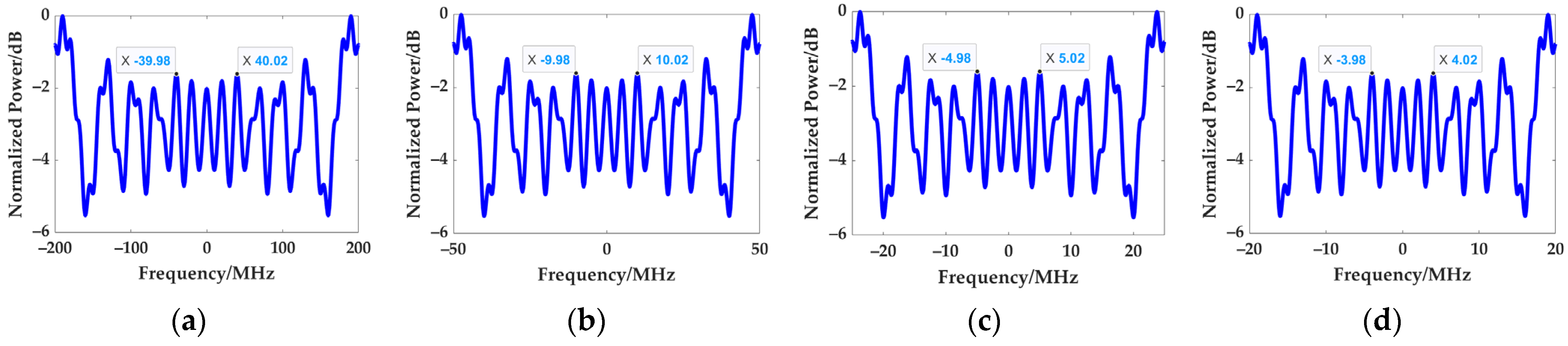
The time-bandwidth product of the LFM pulse is fixed at 50, and the pulse widths are set as 0.1, 0.4, 0.8, and 1 μs. The obtained spectrum amplitudes are illustrated in Figure 10. It can be seen that the amplitude shape around the center of the spectrum is sinusoidal, and the corresponding spectrum fluctuation periods are 20, 5, 2.5, and 2 MHz, respectively, which are consistent with the theoretical derivation. Moreover, as the frequency expands from zero frequency to both sides, the regularity of spectrum fluctuation is reduced gradually. Though the frequencies at the integer multiple of are still the extremal positions of the spectrum, there are several additional peaks with a small amplitude at the non-integer multiple of .
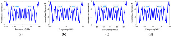
Figure 10.
Spectrum of LFM pulse with the fixed time-bandwidth product of 50 and varying pulse width of: (a) 0.1 μs; (b) 0.4 μs; (c) 0.8 μs; (d) 1 μs.
Second, the effect of stepped frequency on the grating-lobe number in the synthesized HRRP is analyzed.
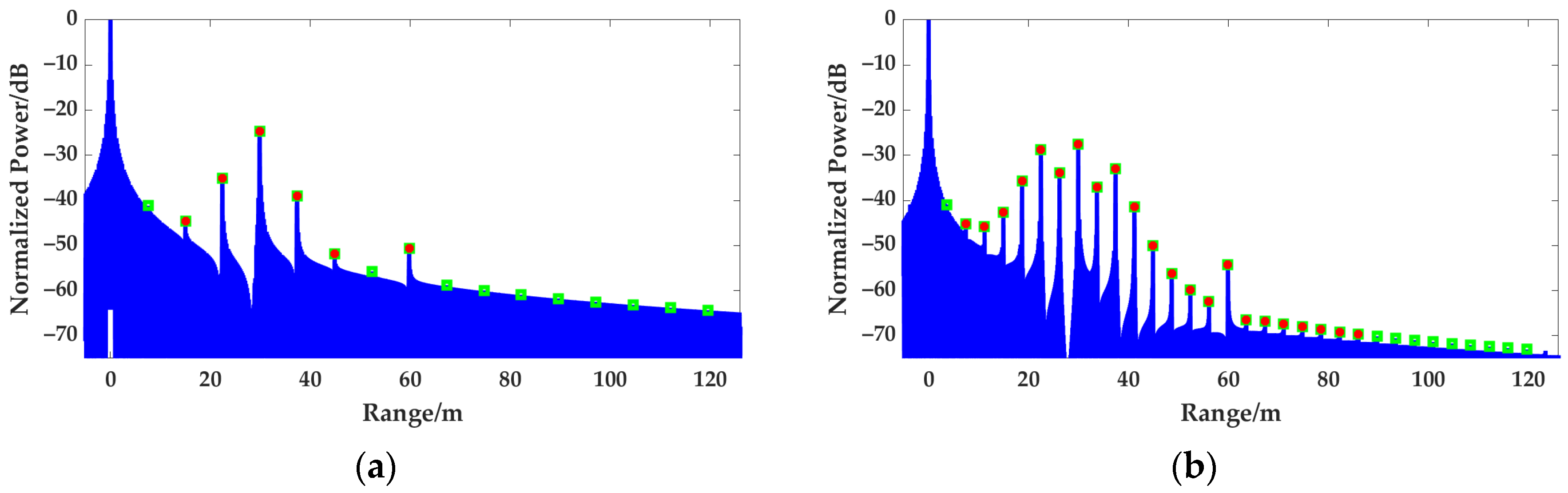
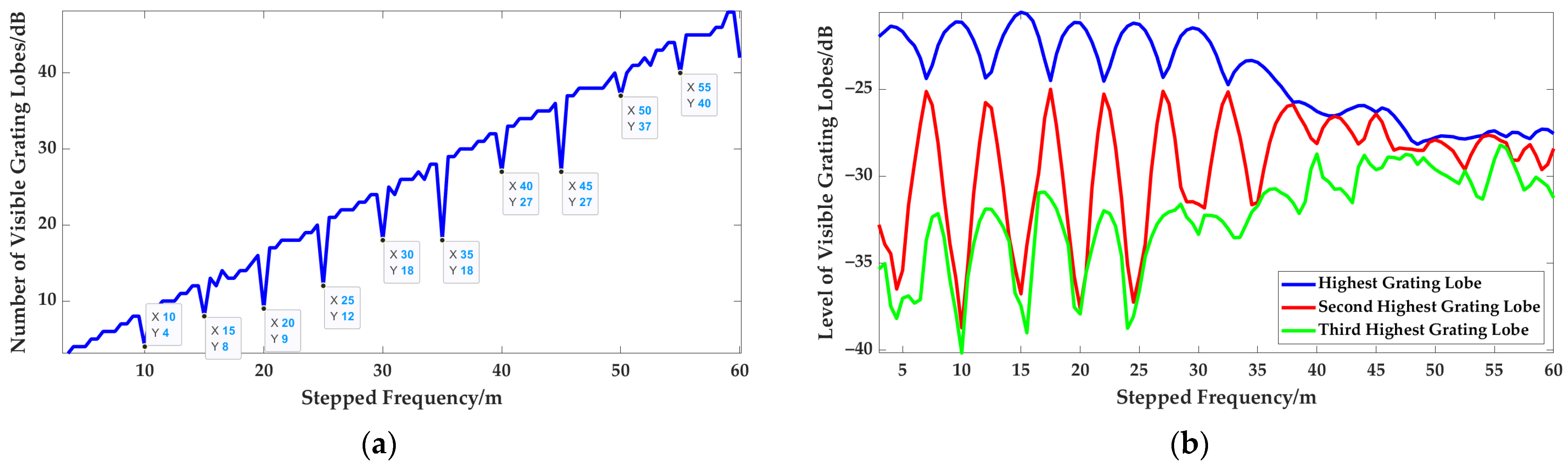
Based on a low blind range FJB waveform with the pulse width of 0.4 μs, the bandwidth of 125 MHz and the subpulse number of 40, the FD-SFP is carried out with the stepped frequencies of 20 and 40 MHz, and the grating-lobe number in the HRRP is counted. Considering a grating lobe will not affect the target detection when its level is lower or close to those of the sidelobes on both sides, the number of the visible grating lobes is introduced as the criteria. Specifically, a grating lobe is set as visible when the level difference is more than 0.5 dB, as shown in the red circle in Figure 11 while all the grating lobes are remarked as the green squares.

Figure 11.
HRRPs with the stepped frequency of: (a) 20 MHz; (b) 40 MHz.
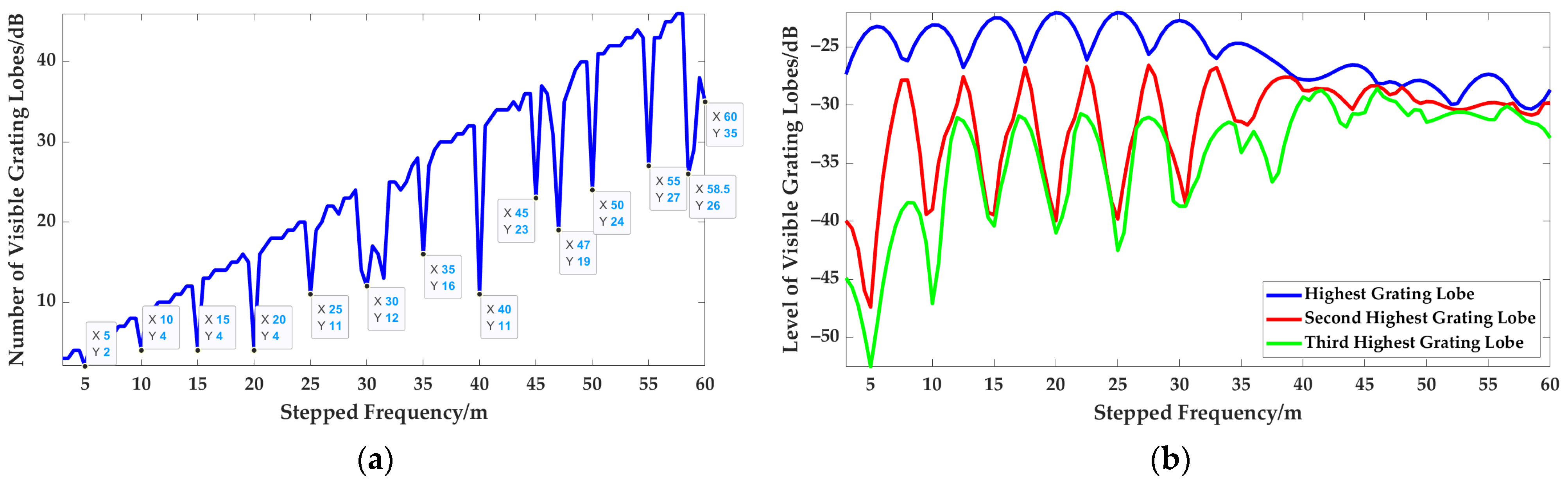
Figure 12a presents the simulated number of visible grating lobes. It shows that the number of visible grating lobes in the HRRP increases gradually with the increase of stepped frequency. However, when the stepped frequency is the integer multiple of the spectrum fluctuation period (5 MHz), the number of visible grating lobes will drop by more than 50%, verifying that the proposed method can reduce the grating-lobe number effectively. In addition, when the stepped frequency is bigger than 30 MHz, the grating-lobe number decreases not only at the integer multiple of 5 MHz but also at some other frequencies such as 47 and 58.5 MHz. This is consistent with the obtained spectrum fluctuation characteristics, in which several additional extremal positions will appear with the increase in the frequency, as shown in Figure 10. Moreover, the level of the peak normalized grating lobe is also simulated, and the result is presented in Figure 12b. When the stepped frequency is the integer multiple of 5 MHz, the highest level of the grating lobe reaches the local maximum. In contrast, the levels of the second and third highest grating lobes are reduced to the local minimum. This finding is identical to the theory analysis, which verifies the proposed method for reducing the grating-lobe number.
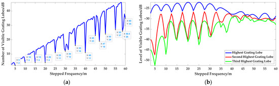
Figure 12.
Simulation results of the effect of step frequency on visible grating lobes: (a) relationship between the number of the visible grating lobes and step frequency; (b) relationship between the levels of the visible grating lobes and step frequency.
Finally, the performance of the grating-lobe level suppression based on Fresnel integral windowing is analyzed.
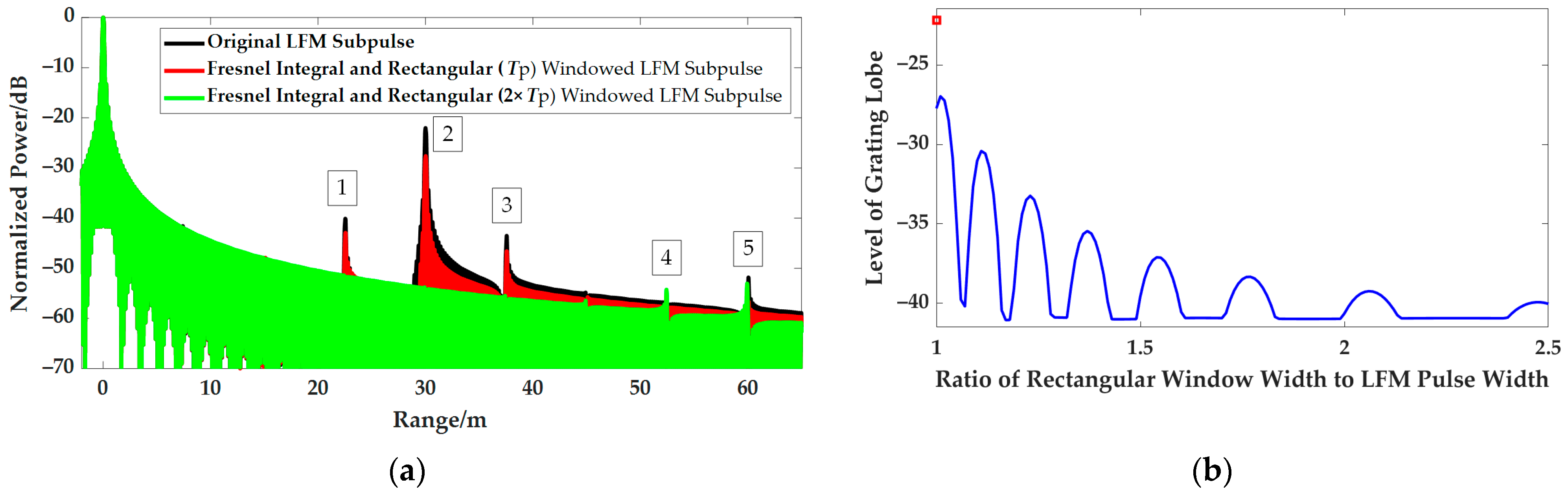
The Fresnel integral window shown in (20) is applied to the FJB waveform mentioned in the previous paragraph, and the rectangular windows with a width of and are superposed respectively to obtain the final transmit signal (Figure 9a). Based on the obtained subpulse, the HRRP with the stepped frequency of 20 MHz is synthesized as shown in Figure 13a, and the corresponding levels of grating lobes are listed in Table 3. It can be seen that based on the Fresnel integral windowed subpulse proposed in this article, the highest grating lobe levels in the HRRP can be reduced by more than 5 dB, which simultaneously realizes the low blind range and low grating-lobe radar detection.
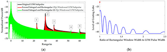
Figure 13.
(a) Synthesized HRRP based on the original and windowed LFM pulses; (b) relationship between the levels of highest grating lobes and the width ratio of the additional rectangular window to LFM pulse with the stepped frequencies.
Table 3.
Grating-lobe levels based on the original LFM subpulse and the proposed windowed LFM subpulse in Figure 13a.
In addition, the width of the additional rectangular window superimposed on the Fresnel integral windowed LFM subpulse is changed to verify its effect on the grating-lobe levels of the HRRP. The relationship between the width of the additional rectangular window and the highest grating-lobe level is presented in Figure 11b, where the red square is the highest grating-lobe level in HRRP synthesized based on the original LFM subpulse. It can be seen that the highest grating-lobe level is significantly reduced by Fresnel integral windowing. Moreover, as the width of the additional rectangular window increases, the highest grating-lobe level first decreases in a fluctuating manner. It then tends to the level of the first grating lobe on either side of the main lobe, i.e., the first grating lobe becomes the highest grating lobe when the width is close to . Furthermore, because the first grating lobe is usually nonvisible, the grating-lobe levels are verified to be effectively suppressed, which is consistent with the theoretical analysis. One final detail remains: when the power amplifier is driven into saturation, the maximum range of amplitude modulation is generally limited. Therefore, the power amplifier performance and the grating-lobe suppression requirement should be balanced when determining the width of the additional rectangular window.
4.2. Experimental Verification
To further verify the effectiveness of the proposed method, based on the high-resolution radar using the FJB waveform with the pulse width of 0.4 μs, the bandwidth of 125 MHz and the stepped number of 40, the metal ball observation experiment was carried out. The corresponding blind range is 60 m, which is lower than the migratory height of insects and meets the taking-off and landing behavior observation requirement. The scenario is shown in Figure 14. A DJI M300 drone was used to hoist the metal ball to 250 m high and 450 m away from the radar. Windless weather was selected specially to ensure a relatively fixed position of the metal ball during the experiment.
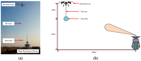
Figure 14.
Metal ball observation experiment scenario: (a) photo; (b) schematic diagram.
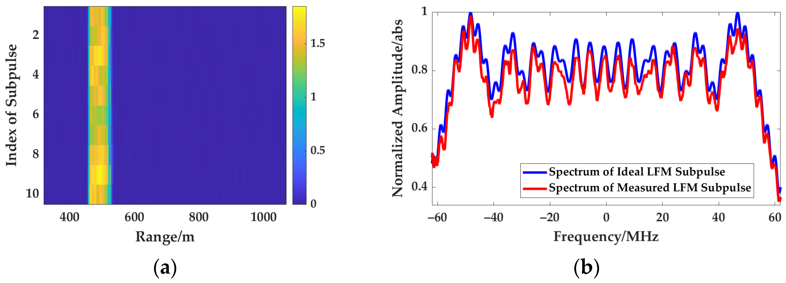
First, the typical LFM subpulse echoes collected by the radar are presented in Figure 15. To verify the grating-lobe number reduction method based on spectrum fluctuation period, since the pulse width of the LFM subpulse is 0.4 μs, based on the conclusion derived in Section 3.2, the spectrum fluctuation period is 5 MHz. The HRRPs are synthesized with varying stepped frequencies, and the number of visible grating lobes and the grating-lobe level are counted, as shown in Figure 16. It can be seen that when the stepped frequency is an integer multiple of 5 MHz, the number of grating lobes in HRRP will decrease significantly. Meanwhile, the highest grating lobe level reaches the local maximum, and those of the second and third grating lobes are in a minimum state, which is consistent with the simulation results. However, the number of visible grating lobes in the experimental verification is greater than that in the simulation. This is mainly affected by the spectrum quality and background noise of the actual waveform.
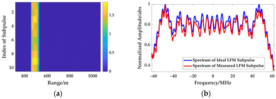
Figure 15.
Subpulse echoes collected by the high-resolution coherent radar: (a) time-domain echoes; (b) spectrum of the ideal and measured LFM subpulse.

Figure 16.
Experimental result of the effect of step frequency on visible grating lobes: (a) relationship between the number of the visible grating lobes and step frequency; (b) relationship between the levels of the visible grating lobes and step frequency.
Next, the grating lobe level reduction based on Fresnel integral windowing is verified.
The transmit LFM subpulse is then modulated by the Fresnel integral window based on (20) and an additional rectangular window with the width of . Based on the above two types of echo, the HRRPs are synthesized with the stepped frequencies of 20 MHz. Moreover, though the magnitude/phase error compensation technologies may change the spectrum characteristics of the insects, it has been widely used in the grating lobe suppression of the FJB waveform; hence the typical error compensation is also considered for the original LFM subpulse in this section. However, the compensation factor is time-varying, leading to a compensation factor extracted from one scene not suitable for another scene. Hence, the error-compensated HRRPs based on the compensation factor from the same and different scenes are also presented. Finally, the obtained HRRPs are shown in Figure 17, and the levels of the grating lobes are listed in Table 4. The results show that most of the grating lobe levels in the HRRP from the Fresnel integral windowed echoes are reduced, and the highest grating lobe level is suppressed by more than 4 dB, which shows the proposed method can achieve the low grating-lobe observation under low blind range. In addition, for the magnitude/phase error compensation method, the error-compensated HRRP based on the compensation factor extracted from the same scene can effectively reduce the grating lobe levels. However, the grating lobes of the error-compensated HRRP based on the different scenes are not suppressed, and most of them are even raised. Therefore, in practice, the frequent extraction of compensation factors in the magnitude/phase error compensation methods is required, which is time consuming and laborious.
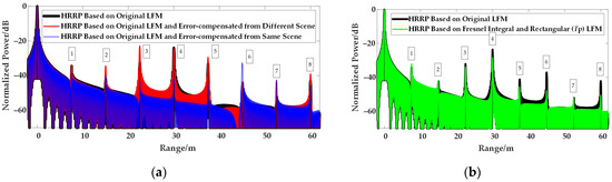
Figure 17.
HRRPs based on the measured LFM subpulse with a stepped frequency of 20 MHz: (a) HRRP based on original LFM subpulse and error-compensated HRRP based on original LFM subpulse from the same/different scene; (b) HRRPs based on original LFM subpulse and Fresnel integral and rectangular windowed LFM subpulse.
Table 4.
Levels of grating lobes of the HRRPs in Figure 17.
5. Application to Insect Taking-Off and Landing Behaviors Observation
In Section 3 and Section 4, the high-resolution and low blind range waveform design methods for insect taking-off and landing behavior observation is discussed in detail. In this section, based on the high-resolution coherent VLR adopting the proposed waveform, the high-resolution flight tracks of the migratory insects are obtained, and their ascent or descent rates are measured by the fitting method similar to [17]. The observation results of insect taking-off and landing behaviors are presented, and the behavior characteristics are analyzed.
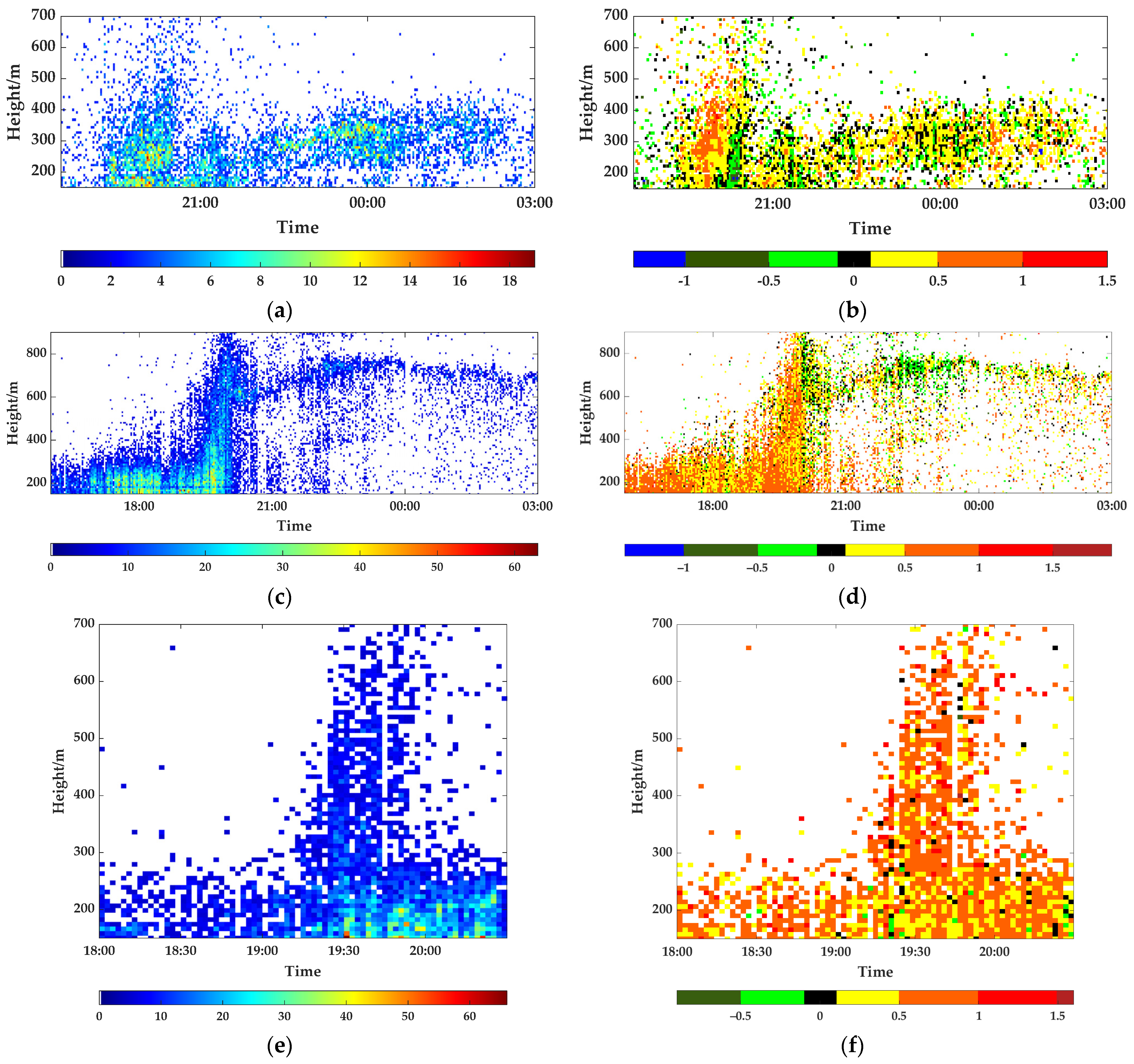
First, three typical taking-off behaviors of the migratory insects were observed on 25–26 July 2020, and 5 March and 24–25 March 2021. The insect information detected by radar was divided into statistical units with a height of 8 m and a time of 2 min. A statistical unit’s ascent or descent rate is calculated as the average of all targets’ rates in the corresponding unit. In addition, the statistical units with less than four insects are eliminated to better demonstrate the statistical pattern of insect flight. The relationships between the insects’ number and the ascent/descent rates with height and time are shown in Figure 18.
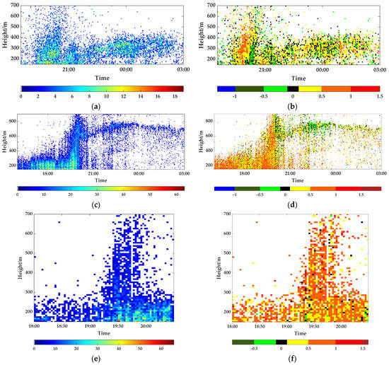
Figure 18.
Relationships between the number and the ascent/descent rates with the height and time for the insects with typical taking-off behavior: (a,b) number and ascent/descent rate distribution with height and time observed on 25–26 July 2020 (sunset occurred at 20:04 h); (c,d) number and ascent/descent rate distribution with height and time observed on 24–25 March 2021 (sunset occurred at 19:25 h); (e,f) number and ascent/descent rate distribution with height and time observed on 5 March 2021 (sunset occurred at 19:17 h).
From the distribution of the insects’ number with height and time in Figure 16a, it can be seen that, between 19:00 and 21:00, the height of dense areas gradually increased with time. Combining the distribution of insects’ ascent or descent rates with height and time in Figure 18b, the ascent rates of migratory insects exceeded +1 m/s between 19:00 and 21:00, indicating that the insects were taking-off at high speed at this time. In addition, the time with the densest insects and highest ascent rates during 19:00~21:00 occurred at around 20:00, which was consistent with the sunset time of 20:04 (China standard time, CST). After 21:00, the height of the migratory insects stabilized between 200 and 400 m. From Figure 18b, the corresponding ascent or descent rates of the swarm were between 0 and 0.5 m/s, indicating that the migratory insects were approaching cruise or turning into a low-speed climbing stage currently.
Similarly, based on the observation results of 24–25 March 2021, shown in Figure 18c,d, many insects took off between 16:00 and 21:00, and the ascent rates were generally greater than 0.5 m/s. The height of the swarm distribution covered almost the whole detection range, and the target numbers in most statistical units are greater than ten from 19:00 to 20:00, which is consistent with the sunset time of 19:25. After 21:00, the insect swarm was observed to concentrate between 600~800 m, and the corresponding ascent/descent rates were between ±0.5 m/s, indicating they were cruising. Moreover, another typical taking-off behavior result observed on 5 March 2021, is presented in Figure 18e,f. It can be seen that the peak period of the insect taking-off was around the sunset time of 19:17, and the ascent rates were between 0.5 and 1 m/s.
Therefore, based on the presented three typical taking-off results, the insect swarms tended to take off around sunset. They were consistent with the insect taking-off behavior pattern that entomologists have analyzed, thus further verifying the proposed waveform design methods in outfield applications.
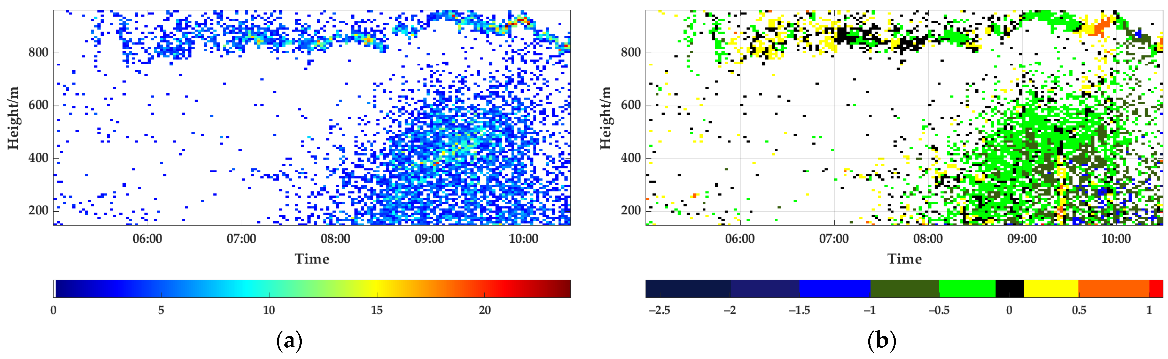
In addition to the taking-off behaviors, the typical insect cruising and landing behaviors were also observed on 9–10 July 2021. Adopting the same analysis method as Figure 18, the relationships between the migratory insects’ number and the ascent/descent rates with height and time were obtained, as shown in Figure 19. It can be seen that there were two insect swarms detected in turn. The first insect swarm was detected between 6:00 and 10:00 by VLR, and its flight height was concentrated at around 850 m. The ascent/descent rates of most corresponding statistical units were measured between −0.5 and 0.5 m/s, thus indicating the insects were cruising. A second insect swarm appeared after 8:00 and was distributed in the airspace below 750 m. Their descent rates were measured mostly between −1.0 and −0.1 m/s, and up to −1.5 m/s at low height. It proves that the insect swarm was in a landing state.
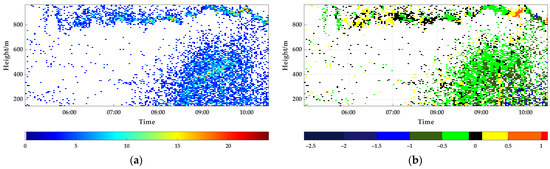
Figure 19.
Relationships between the number and the ascent/descent rates with the height and time for insects with typical landing behavior: (a) distribution of number with height and time; (b) distribution of ascent/descent rate with height and time. The sunrise occurred at 04:54 h.
6. Discussion
The FJB waveform is optimal for realizing the high-resolution and low blind range measurement of migratory insects. However, the high grating lobes in the HRRP may cause the missed detection of the tiny insects, particularly when the blind range is small. To suppress the grating lobes, two main methods, namely waveform design and signal processing methods, have been proposed. The signal processing methods restructure the synthesized wideband spectrum into the desired shape to reduce the grating lobe. These methods will change the scattering characteristics of the targets and further affect the extraction precision of the insect body parameters. In addition, current waveform design methods are mainly based on the ACF, which is not suitable for the widely used FD-SFP.
In this paper, the low blind range and low grating-lobe FJB waveform design methods are proposed, which are not based on the ACF but on the spectrum fluctuation characteristics under the small pulse width. The precise spectrum of the narrow-band LFM subpulse is modeled for the first time based on the Fresnel integral and its approximation. Then, an innovative method is proposed to reduce the grating-lobe number by ensuring the continuity of the synthesized spectrum and to decrease the grating-lobe levels by suppressing the spectrum fluctuation in a time-domain windowing way.
The simulation and experiment results proved that the proposed method can effectively reduce the number and levels of grating lobes under the small pulse width. In addition, by comparing the results of simulation and field experiment, the proposed method in the practical application meets the requirement for the signal quality of the radar emitted waveform. The actual spectrum fluctuation should be similar to the theoretical value to allow the errors to be compensated for. In addition, for the grating-lobe level suppression method based on the Fresnel integral windowing, limited by some power amplifiers used in the radars, an additional rectangular window in the time domain may be needed to reduce the amplitude fluctuation of the power amplifier with saturated output. This will reduce the performance to a certain extent. However, in some other application scenarios where high-power saturation output is not required, such as communications, this additional rectangular window may be avoidable; hence the grating lobes can be further suppressed to a lower level.
7. Conclusions
High-resolution and low blind range measurements of migratory insects are important for their taking-off and landing behavior observation. The range resolutions of current VLRs are between 7.5 and 15 m, and the blind range is higher than 150 m, making it difficult to precisely observe the flight behavior of low-altitude insects. In this paper, the high-resolution, low blind range FJB waveform design methods for migratory insects’ taking-off/landing behavior observation are proposed. First, based on the measured data collected by a high-resolution coherent VLR in the outfield, the spatial spacings of the insect flight tracks are obtained for the first time, and the waveform design requirement is analyzed, thereby validating the need for the high-resolution and low blind range observation. The results also prove that the range resolution of VLRs should be better than 3.3 m to distinguish more than 95% of closely spaced individual insects. Second, the FJB waveform is found to be the optimal choice for the high-resolution and low blind range observation of migratory insects, but its inherently periodic grating-lobe problem becomes an obstacle to further application. Considering the grating lobes of the FJB waveform are mainly caused by the amplitude fluctuation in the spectrum of narrow-band LFM subpulse, the spectrum model is derived based on the Fresnel integral and its approximation for the first time. On this basis, the low blind range and low grating-lobe FJB waveform design methods based on the spectrum fluctuation period and the Fresnel integral windowing are proposed to reduce the number and levels of the grating lobes, respectively. Third, the simulation and experiment are carried out to verify the performance of the proposed waveform. The result shows that the grating-lobe number can be reduced to 50%, and the highest grating-lobe level is suppressed by more than 4 dB. Finally, the proposed method is applied to the taking-off/landing behaviors observation of migratory insects. Typical observation results of the taking-off and landing behaviors are presented. The results prove that the insects usually take off around sunset, consistent with the existing conclusions.
Author Contributions
Conceptualization, R.W. and T.Z.; methodology, T.Z.; software, K.C. and T.Y.; validation, Q.J. and R.Z.; formal analysis, R.W.; investigation, T.Z.; resources, K.C.; data curation, J.L.; writing—original draft preparation, R.W. and T.Z.; writing—review and editing, R.W. and T.Z.; visualization, T.Y. and J.L.; supervision, C.H. and J.L.; project administration, Q.J.; funding acquisition, R.W. and C.H. All authors have read and agreed to the published version of the manuscript.
Funding
This research was funded by the National Natural Science Foundation of China (Grant No. 31727901) and the National Natural Science Foundation of China (Grant No. 62001021).
Data Availability Statement
Not applicable.
Conflicts of Interest
The authors declare no conflict of interest.
References
- Altizer, S.; Bartel, R.; Han, B.A. Animal Migration and Infectious Disease Risk. Science 2011, 331, 296–302. [Google Scholar] [CrossRef] [PubMed] [Green Version]
- Hu, G.; Lim, K.S.; Horvitz, N.; Clark, S.J.; Reynolds, D.R.; Sapir, N.; Chapman, J.W. Mass seasonal bioflows of high-flying insect migrants. Science 2016, 354, 1584–1587. [Google Scholar] [CrossRef] [PubMed] [Green Version]
- Vaughn, C.R. Birds and insects as radar targets: A review. Proc. IEEE 1985, 73, 205–227. [Google Scholar] [CrossRef]
- Riley, J.R. Radar cross section of insects. Proc. IEEE 1985, 73, 228–232. [Google Scholar] [CrossRef]
- Aldhous, A.C. An Investigation of the Polarisation Dependence of Insect Radar Cross Sections at Constant Aspect. Ph.D. Thesis, Cranfield University, Bedford, UK, 1989. [Google Scholar]
- Drake, V.A.; Reynolds, D. Insects as radar targets. In Radar Entomology: Observing Insect Flight and Migration, 1st ed.; CABI: São Paulo, Brazil, 2012. [Google Scholar] [CrossRef]
- Wang, R.; Hu, C.; Liu, C.; Long, T.; Kong, S.; Lang, T.; Gould, P.J.L.; Lim, J.; Wu, K. Migratory Insect Multifrequency Radar Cross Sections for Morphological Parameter Estimation. IEEE Trans. Geosci. Remote Sens. 2019, 57, 3450–3461. [Google Scholar] [CrossRef]
- Drake, V.A.; Chapman, J.W.; Lim, K.S.; Reynolds, D.R.; Riley, J.R.; Smith, A.D. Ventral-aspect radar cross sections and polarization patterns of insects at X band and their relation to size and form. Int. J. Remote Sens. 2017, 38, 5022–5044. [Google Scholar] [CrossRef]
- Riley, J.R. Collective orientation in night-flying insects. Nature 1975, 253, 113–114. [Google Scholar] [CrossRef]
- Chapman, J.W.; Smith, A.D.; Woiwod, I.P.; Reynolds, D.R.; Riley, J.R. Development of vertical-looking radar technology for monitoring insect migration. Comput. Electron. Agric. 2002, 35, 95–110. [Google Scholar] [CrossRef]
- Riley, J.R.; Reynolds, D.R. Orientation at Night by High-Flying Insects. Insect Flight; Springer: New York, NY, USA, 1986; pp. 71–87. [Google Scholar] [CrossRef]
- Wolf, W.W.; Westbrook, J.K.; Raulston, J.; Pair, S.D.; Hobbs, S.E. Recent airborne radar observations of migrant pests in the United States. Philos. Trans. R. Soc. Lond. B Biol. Sci. 1990, 328, 619–630. [Google Scholar] [CrossRef]
- Riley, J.R.; Smith, A.D.; Reynolds, D.R.; Edwards, A.S.; Osborne, J.L.; Williams, I.H.; Carreck, N.L.; Poppy, G.M. Tracking bees with harmonic radar. Nature 1996, 379, 29–30. [Google Scholar] [CrossRef]
- Chapman, J.W.; Reynolds, D.R.; Smith, A.D. Vertical-looking radar: A new tool for monitoring high-altitude insect migration. BioScience 2003, 53, 503–511. [Google Scholar] [CrossRef] [Green Version]
- Smith, A.D.; Riley, J.R.; Gregory, R.D. A Method for Routine Monitoring of the Aerial Migration of Insects by Using a Vertical-Looking Radar. Philos. Trans. R. Soc. Lond. Ser. B Biol. Sci. 1993, 340, 393–404. [Google Scholar] [CrossRef]
- Harman, I.T.; Drake, V.A. Insect monitoring radar: Analytical time-domain algorithm for retrieving trajectory and target parameters. Comput. Electron. Agric. 2004, 43, 23–41. [Google Scholar] [CrossRef]
- Drake, V.A.; Wang, H. Ascent and descent rates of high-flying insect migrants determined with a non-coherent vertical-beam entomological radar. Int. J. Remote Sens. 2018, 40, 883–904. [Google Scholar] [CrossRef]
- Drake, V.A.; Hatty, S.; Symons, C.; Wang, H. Insect Monitoring Radar: Maximizing Performance and Utility. Remote Sens. 2020, 12, 596. [Google Scholar] [CrossRef] [Green Version]
- Zhou, C.; Wang, R.; Hu, C. Equivalent point estimation for small target groups tracking based on maximum group likelihood estimation. Sci. China Inf. Sci. 2020, 63, 1–3. [Google Scholar] [CrossRef]
- Wang, R.; Cai, J.; Hu, C.; Zhou, C.; Zhang, T. A Novel Radar Detection Method for Sensing Tiny and Maneuvering Insect Migrants. Remote Sens. 2020, 12, 3238. [Google Scholar] [CrossRef]
- Wang, R.; Zhang, Y.; Tian, W.; Cai, J.; Hu, C.; Zhang, T. Fast implementation of insect multi-target detection based on multimodal optimization. Remote Sens. 2021, 13, 594. [Google Scholar] [CrossRef]
- Smith, A.D.; Riley, J.R. Signal processing in a novel radar system for monitoring insect migration. Comput. Electron. Agric. 1996, 15, 267–278. [Google Scholar] [CrossRef]
- Drake, V.A. Signal processing for ZLC-configuration insect-monitoring radars: Yields and sample biases. In Proceedings of the 2013 International Conference on Radar, Ottawa, ON, Canada, 29 April–3 May 2013; pp. 298–303. [Google Scholar] [CrossRef]
- Wang, R.; Zhang, T.; Hu, C.; Cai, J.; Li, W. Digital Detection and Tracking of Tiny Migratory Insects Using Vertical-Looking Radar and Ascent and Descent Rate Observation. IEEE Trans. Geosci. Remote Sens. 2021, 60, 1–15. [Google Scholar] [CrossRef]
- Beerwinkle, K.R.; Witz, J.A.; Schleider, P.G. An automated, vertical looking, X-band radar system for continuously monitoring aerial insect activity. Trans. ASAE 1993, 36, 965–970. [Google Scholar] [CrossRef]
- Smith, A.D.; Reynolds, D.R.; Riley, J.R. The use of vertical-looking radar to continuously monitor the insect fauna flying at altitude over southern England. Bull. Entomol. Res. 2000, 90, 265–277. [Google Scholar] [CrossRef] [PubMed]
- Levanon, N.; Mozeson, E. Coherent Train of LFM Pulses. In Radar Signals; John Wiley & Sons, Inc.: Hoboken, NJ, USA, 2004. [Google Scholar] [CrossRef]
- Hai-bin, L.; Yun-hua, Z.; Jie, W. Sidelobes and grating lobes reduction of stepped-frequency chirp signal. In Proceedings of the 2005 IEEE International Symposium on Microwave, Antenna, Propagation and EMC Technologies for Wireless Communications, Beijing, China, 8–12 August 2005; Volume 2, pp. 1210–1213. [Google Scholar] [CrossRef]
- Xu, S.; Tian, W.; Sun, L.; Yao, D.; Zeng, T. Grating lobes suppression technique in stepped chirp radar. In Proceedings of the IET International Radar Conference, Xi’an, China, 14–16 April 2013. [Google Scholar] [CrossRef]
- Ding, Z.; Gao, W.; Liu, J.; Zeng, T.; Long, T. A novel range grating lobe suppression method based on the stepped-frequency SAR image. IEEE Geosci. Remote Sens. Lett. 2014, 12, 606–610. [Google Scholar] [CrossRef]
- Zeng, T.; Mao, C.; Hu, C.; Zhu, M.; Tian, W.; Ren, J. Grating lobes suppression method for stepped frequency GB-SAR system. J. Syst. Eng. Electron. 2014, 25, 987–995. [Google Scholar] [CrossRef]
- Ding, Z.; Guo, Y.; Gao, W.; Kang, Q.; Zeng, T.; Long, T. A range grating lobes suppression method for stepped-frequency SAR imagery. IEEE J. Sel. Top. Appl. Earth Obs. Remote Sens. 2016, 9, 5677–5687. [Google Scholar] [CrossRef]
- Levanon, N.; Mozeson, E. Nullifying ACF grating lobes in stepped-frequency train of LFM pulses. IEEE Trans. Aerosp. Electron. Syst. 2003, 39, 694–703. [Google Scholar] [CrossRef]
- Gladkova, I.; Chebanov, D. Grating lobes suppression in stepped-frequency pulse train. IEEE Trans. Aerosp. Electron. Syst. 2008, 44, 1265–1275. [Google Scholar] [CrossRef]
- Gladkova, I. Analysis of stepped-frequency pulse train design. IEEE Trans. Aerosp. Electron. Syst. 2009, 45, 1251–1261. [Google Scholar] [CrossRef]
- Gladkova, I.; Chebanov, D. Suppression of grating lobes in stepped-frequency train. In Proceedings of the IEEE International Radar Conference, Arlington, VA, USA, 9–12 May 2005; pp. 371–376. [Google Scholar] [CrossRef] [Green Version]
- Gladkova, I. A general class of stepped frequency trains. In Proceedings of the 2006 IEEE Conference on Radar, Shanghai, China, 24–27 April 2006; Volume 6. [Google Scholar] [CrossRef]
- Kumar, V.; Sahoo, A.K. Grating lobe and sidelobe suppression using Multi-Objective Optimization Techniques. In Proceedings of the International Conference on Communications and Signal Processing (ICCSP), Tamilnadu, India, 2–4 April 2015; pp. 247–251. [Google Scholar] [CrossRef]
- Kumar, V.; Sahoo, A.K. Side lobe and grating lobe suppression in stepped frequency pulse train using multi-objective optimization algorithms. In Proceedings of the 2016 International Conference on Advances in Computing, Communication, & Automation (ICACCA) (Spring), Dehradun, India, 30 September–1 October 2016; pp. 1–6. [Google Scholar] [CrossRef]
- Lord, R.T.; Inggs, M.R. High resolution SAR processing using stepped-frequencies. IEEE Int. Geosci. Remote Sens. 1997, 1, 490–492. [Google Scholar] [CrossRef]
- Wilkinson, A.J.; Lord, R.T.; Inggs, M.R. Stepped-frequency processing by reconstruction of target reflectivity spectrum. In Proceedings of the 1998 South African Symposium on Communications and Signal Processing-COMSIG’98 (Cat. No. 98EX214), Rondebosch, South Africa, 7–8 September 1998; pp. 101–104. [Google Scholar] [CrossRef]
- Nel, W.; Tait, J.; Lord, R.; Wilkinson, A. The use of a frequency domain stepped frequency technique to obtain high range resolution on the CSIR X-band SAR system. In Proceedings of the IEEE AFRICON. 6th Africon Conference in Africa, George, South Africa, 2–4 October 2002; pp. 327–332. [Google Scholar] [CrossRef]
- Richards, M.A. Doppler Processing and Constant False Alarm Rate (CFAR) Detection. In Fundamentals of Radar Signal Processing; McGraw-Hill Education: New York, NY, USA, 2014. [Google Scholar]
- Kowatsch, M.; Stocker, H.R. Effect of Fresnel ripples on sidelobe suppression in low time-bandwidth product linear FM pulse compression. IET Digital Library. IEE Proc. F Commun. Radar Signal Process. 1982, 129, 41–44. [Google Scholar] [CrossRef]
- Heald, M.A. Rational approximations for the Fresnel integrals. Math. Comput. 1985, 44, 459–461. [Google Scholar] [CrossRef]


Publisher’s Note: MDPI stays neutral with regard to jurisdictional claims in published maps and institutional affiliations. |
© 2022 by the authors. Licensee MDPI, Basel, Switzerland. This article is an open access article distributed under the terms and conditions of the Creative Commons Attribution (CC BY) license (https://creativecommons.org/licenses/by/4.0/).