Abstract
In this paper, we discuss different approaches to optimal sensor placement and propose that an optimal sensor location can be selected using unsupervised learning methods such as self-organising maps, neural gas or the K-means algorithm. We show how each of the algorithms can be used for this purpose and that additional constraints such as distance from shore, which is presumed to be related to deployment and maintenance costs, can be considered. The study uses wind data over the Mediterranean Sea and uses the reconstruction error to evaluate sensor location selection. The reconstruction error shows that results deteriorate when additional constraints are added to the equation. However, it is also shown that a small fraction of the data is sufficient to reconstruct wind data over a larger geographic area with an error comparable to that of a meteorological model. The results are confirmed by several experiments and are consistent with the results of previous studies.
1. Introduction
When faced with the problem of selecting a site for sensor placement, one usually asks how this can be done in an “optimal” way. Phrasing the question this way, one might tacitly assume that it is an optimisation problem. This assumption could direct our search for a solution to the definition of a criterion that defines “optimal” and enables a search for an optimal solution. In most cases, the optimisation criterion is related to the budget in one way or another. For example, one might try to optimise sensor cost by finding the smallest number of sensors with the greatest coverage. Or one could optimise the total cost of a measuring endeavour by including deployment and maintenance costs. Alternatively, the problem can be formulated as an optimization problem with constraints, where a budget or a certain number of sensors is an additional constraint. In such scenarios, the constraint might be some other scarce resource (e.g., energy) rather than budget, but coverage or even accuracy of measurements is the primary concern. Much previous work falls into this category, and one could say that this describes a traditional approach in which optimal sensor placement is treated as an optimisation problem [1,2,3]. However, we will not only treat the optimal sensor location problem as an optimisation problem, but also discuss an alternative in which we treat the optimal sensor location problem as a feature selection problem. Next, we will propose that classical clustering approaches can be used for sensor location selection.
The optimal sensor placement problem could also be approached differently, asking whether there are certain locations that are better suited for data collection. This problem could be called a selection problem rather than an optimisation problem. In this case, the question is whether a particular site (out of a set of available sites) is more suitable than another. An attentive reader will already notice a similarity between this problem and a feature selection problem. We should also note that the selection problem uses a criterion by which the selection is made. Recently, the quality of reconstruction also emerged as a new criterion for feature selection [4,5,6]. Regardless of whether we observe this problem in terms of sensor (site) selection or optimal sensor placement, we can find a number of proposed solution [7,8,9,10,11,12,13]. This is even more true when we consider the different feature selection algorithms available (e.g., [14,15,16,17]).
The main motivation for this paper comes from our recent work [18,19]. There we have already shown that it is possible to intelligently select locations for sensor placement—and we have shown that it is possible to use a clustering algorithm to achieve this. As mentioned earlier, various criteria can be used to select features. Similarly, feature selection algorithms can be supervised or unsupervised. In a supervised settings, if the true value is available, the most natural approach would be to maximise feature relevance with respect to a true value that can be measured, for example, by the reconstruction error. On the other hand, if the true value is not available and an unsupervised setting is used, the natural criterion for feature selection would be to minimise feature redundancy and maximise feature relevance [20]. If the true value is not available, feature relevance can be measured as coherence between similar features. To minimise feature redundancy, one can also try to reduce the number of similar features. Note that the unsupervised clustering approach does exactly this, as it partitions the datasets into sets such that the distance between sets is maximised and the distance within the set is minimised. Therefore, in this paper, we will compare three different clustering algorithms to show that it is possible to achieve feature selection using different algorithms. We will also evaluate which algorithm provides the best sensor locations in terms of reconstruction error. In addition, we will explore the possibility of selecting the optimal sensor location by introducing other criteria, such as distance to shore, which is likely related to deployment and maintenance costs. Of course, other variants are also possible.
The clustering methods described in the following sections are (a) Self-organising maps (SOM), also known as Kohonen maps or Kohonen neural network [21,22], (b) Neural gas [23], in particular the implementation known as Growing neural gas (GNG) [24] and (c) K-means clustering [20,25]. It is not uncommon to find applications of these algorithms in geosciences. For example, neural gas has been used in marine microbial diversity detection [26] and self-organising maps have been used to detect biogeochemical property dynamics [27], spatiotemporal reproducibility of microbial food web structure [28], find teleconnection patterns between precipitation [29] and toxic phytoplankton species [30], or classify wind patterns [31,32,33,34,35]. Several papers (e.g., [27,28]) have used K-means in addition to SOM.
2. Data
The section describes both the source of the data and the data wrangling necessary for further experiments. By the end of the section we also describe how we divided the data set into a training set and a test set and how the dependent and independent variables were defined.
The data used in this study are from Copernicus Climate Change Service information and include ERA5 wind vector data. ERA5 is the new reanalysis produced by the European Centre for Medium-range Weather Forecasts (ECMWF) as part of the Copernicus Climate Change Service [36]. ERA5 is the fifth generation of reanalysis produced by using 4D-Var data assimilation in combination with atmospheric forecasts. The reanalysis combines atmospheric models with all available observations to produce the best numerical estimate of past climate. The state-of-the-art ERA5 reanalysis provides atmospheric, land surface, and ocean wave variables with a horizontal resolution of 31 km and hourly output. To obtain the wind data for the Mediterranean Sea, the area from N to N latitude and from E to E longitude was extracted. From this area, data were sampled at a resolution of and land-sea masking was applied to the total number of sampled points to obtain only the wet points. The points outside the Mediterranean Sea were manually removed so that the final result covers the Mediterranean Sea area with a total of 1244 points. This area is shown in Figure 1.
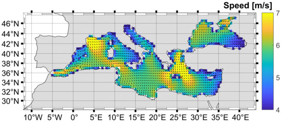
Figure 1.
Mediterranean Sea. The figure shows the average wind over the Mediterranean Sea, with the vector indicating the direction and the color indicating the intensity.
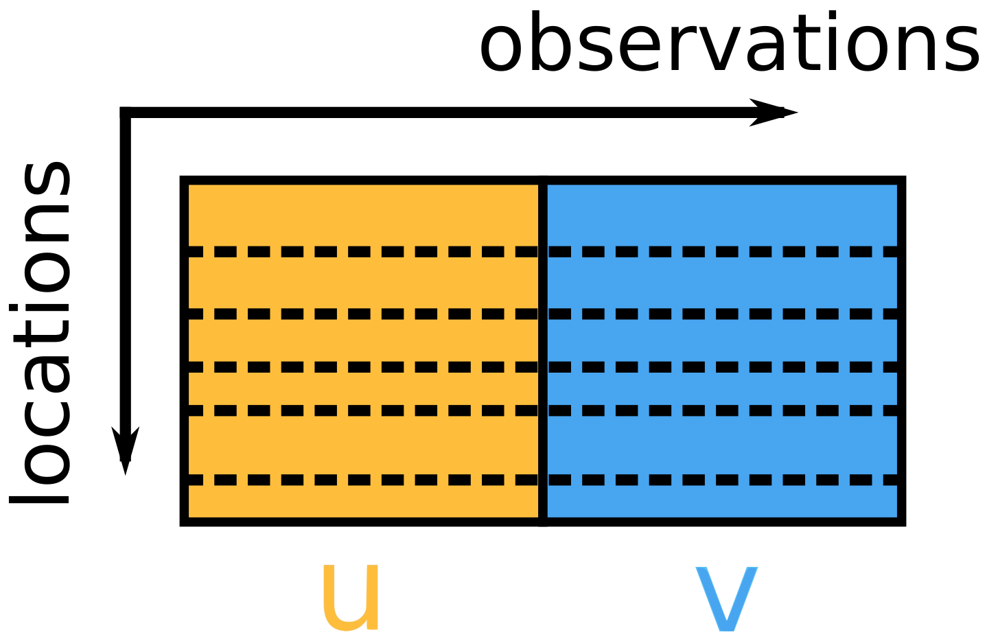
A total of 1244 points were collected in the area shown in Figure 1 and wind data were obtained from these sites and used in our study. The data were collected for the period 1979–2019 at a time interval of 6 h. The data are then organised as a 1244-by-179700 matrix. Each row represents a spatial data vector that contains all spatial information collected at a given time. The data vector contains the concatenated u and v information of the wind vector components. Here, u and v are measured at 10 m above sea level and expressed in metres per second. They denote the west-east and south-north wind components, respectively. After data wrangling the data matrix used for further processing has the form shown in Figure 2.

Figure 2.
Matrix of input data. The dashed lines indicate the rows of the matrix containing the data collected at the optimal sensor location.
In the following section, we will describe three methods for selecting the rows marked with dashed lines in Figure 2. Note that the selected rows uniquely define the locations for sensor placement and that this location selection is based on observations of both channel u and v.
To evaluate the clustering methods used to determine the optimal locations for sensor placement, we measure the reconstruction error for each subset of the sensor locations determined in each experiment. The reconstruction problem is a supervised learning problem. Therefore, we need to divide the data into a training set and a test set and define the dependent and independent variables. The training and test sets are split 80:20 by randomly selecting the available data at different time points. The independent variables (input variables to the model) would be the observations at selected locations and the observations from all other locations would be the dependent variables. Note that the dependent and independent variables would vary across experiments. To measure the error, the evaluation is performed on the test set using the true values of the dependent variables as the gold standard.
3. Methods
In this section, we first describe three learning methods that are typically used for clustering. Later in the paper, these methods are used to identify optimal locations for sensor placement. Following the description of the methods, we briefly describe two data reconstruction models required for evaluating sensor location selection based on reconstruction error. At the very end of the section, we will also describe the error measure used to quantify the reconstruction error. The remainder of the section is therefore divided into six parts, each describing a topic: (a) K-means clustering, (b) Growing neural gas (GNG), (c) Self-organising maps (SOM), (d) K-nearest neighbours, (e) linear regression, and (f) reconstruction error.
The idea of using clustering methods to determine the optimal location for sensor placement is based on the premise that data would naturally agglomerate in space, since proximity coincides with correlation in virtually all natural processes. Clustering methods are suitable for the optimal sensor placement problem because they not only partition the data set into clusters, but also provide cluster centres, also referred to as “winning neurons” or “best-matching units” (BMUs) in GNG and SOM, and represented by their weights or codebook vectors. Note that for each cluster, the cluster centre can be considered as the most representative data point and the sensor that generates the most representative data is the optimal sensor. All three methods have a drawback: they update the cluster centre by averaging the values of the surrounding data. This approach may seem obvious and straightforward, but such a solution is often not an instance from a sample set. However, we would prefer to identify an instance that belongs to a set of available locations for sensor placement. This problem is not uncommon and some algorithms address it by using the median instead of the mean. To address this issue and ensure that the optimal sensor location is selected from the set of predefined locations, we implemented a modification to the existing algorithm that updates the cluster centre to the closest available location for sensor placement.
3.1. K-Means
We begin by describing how the K-means algorithm updates cluster centres. In this and subsequent sections, we will use the notation to denote the cluster centre or neuron/BMU weights. While we are aware that it is not common practise to use the notation when describing the K-means algorithm, we make an exception here to highlight the similarities between the algorithms described here so that important differences between the algorithms are more apparent.
The K-means algorithm requires only one parameter (K), which specifies the number of clusters, and uses an iterative process to update the BMUs such that the variation within a cluster is minimised for each cluster. Using the notation for within-a-cluster variation, and for the BMU of the kth cluster, we can say that the optimisation problem the algorithm is trying to solve is:
To solve the problem, one needs to define , and since denotes the distance of elements within a cluster, the easiest way would be to calculate the Euclidean distance between all elements of a cluster. To ensure that larger clusters do not overweight the smaller ones, one could also normalise the result to the number of elements in the cluster. The complexity of the problem (there are ways to partition a set of n elements into K subsets) motivates us to use the learning algorithm to solve the problem. The adaptation step can be described by a Hebb’s learning procedure that minimises the Euclidean distance via a stochastic gradient descent algorithm:
where is the step size and is the Kronecker delta, where k denotes the cluster to which and belong. The denotes the ith instance of the sensor s, and whether it belongs to the cluster k is defined by the Voronoi polygon, and the Kronecker delta determines how it affects the result.
This online learning approach can be further modified by organising the data into batches where each cluster is a separate batch. Such an algorithm computes the centres of each cluster (let us denote them by ) and updates the BMU towards that centre, which can be faster:
This simple clustering algorithm is known to converge to a local optimum. Nevertheless, it is often used because it generally gives good results. To solve this problem, one can use a soft-max adaptation rule that adjusts not only one BMU, but also other BMUs based on their proximity.
3.2. Growing Neural Gas
Neural gas (NG) can be considered a modification of online K-means clustering because its adaptation step uses a slightly different postsynaptic excitation function:
where denotes adaptation step and is the ranking of vectors in the neighborhood of . The function is typically chosen as follows:
where denotes the so-called “neighbourhood area” that determines the number of neighbouring neurons that adapt together with the BMU. The use of instead of results in the algorithm updating not only one but also its neighbours at each update. This can be interpreted to mean that there is a “loose” connection between the BMU and the neighbouring BMUs that has gas-like dynamics, or as Maritnetz et al. put it in [23]: the dynamics of the BMUs can be described as particle motion in a potential field, where the potential is given as a negative data point density. We refer to the connection between BMUs as a “loose” connection, since the neighbourhood is defined based on the distance between the units (i.e., the rank) and therefore can be changed as the algorithm learns (as the BMUs move in space). Note that this is in contrast to the “strict” definition of neighbours, where the predefined neighbours of each BMU do not change with the iterations of the algorithm—as we will see in a moment, this is the case with the SOM algorithm. Because of these properties, the algorithm has earned the name neural gas. The algorithm has one advantage over the K-means algorithm, namely its ability to capture the manifold structure of the underlying data. This property is shared by NG with the SOM algorithm and will be described in more detail later along with the SOM algorithm. On the other hand, the NG algorithm is similar to the K-means algorithm in that it has fixed k centres that it optimises, and—similar to K-means—the initial selection for k may be suboptimal. This is avoided by a modification of the NG algorithm proposed by Fritzke [24]. The algorithm is called Growing Neural Gas (GNG) because the number of BMUs grows from the initial number of clusters () to the maximum number of clusters ().
As an overall evaluation of the algorithm, it can be said (see [23]) that neural gas (including GNG) exhibits faster convergence with smaller distortion errors, but consumes more computational power, especially for ranking (sorting).
3.3. Self-Organising Map
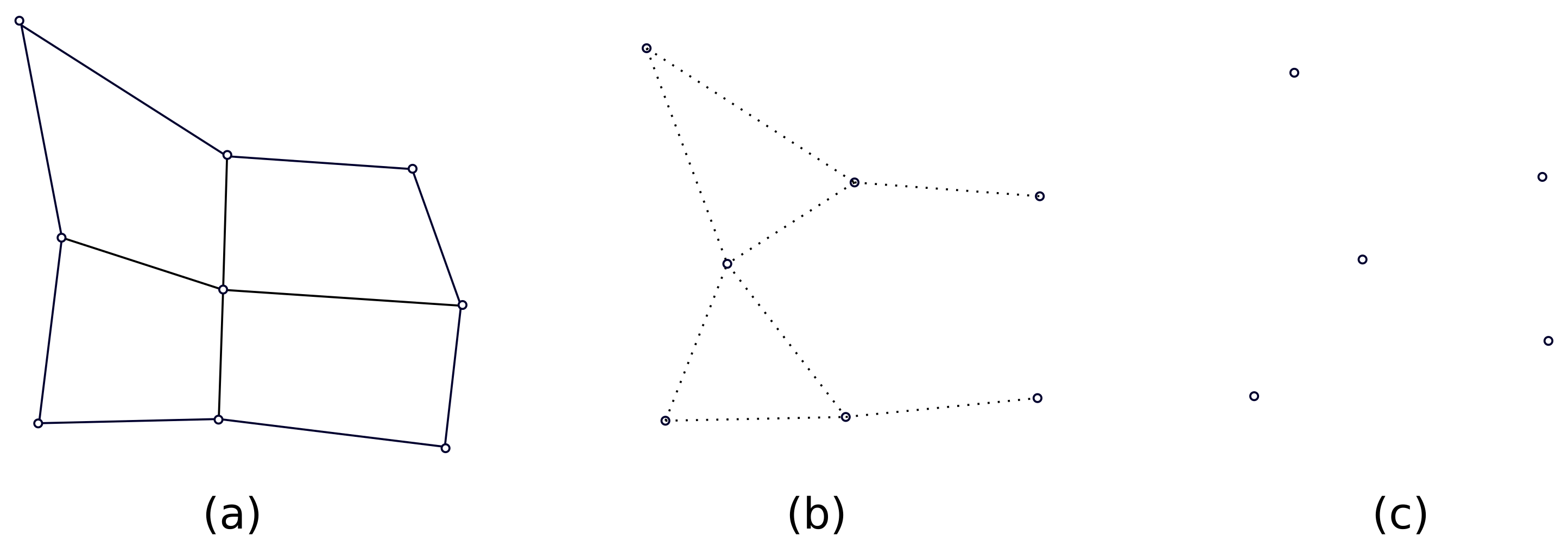
Historically, self-organising maps (SOM) precede both GNG and NG algorithms [21,22]. However, we believe it is appropriate to introduce them in this order when we introduce the notion of lattice. In SOM, the lattice describes the predefined topological structure between BMUs. This structure is usually (but not necessarily) 2D and of rectangular shape, and all BMUs have up to four neighbours (due to the rectangular lattice structure, only BMUs at the lattice edge have less than four neighbours). Compared to (G) NG or K-means, the lattice structure of SOM is regular and strict, while GNG and K-means have irregular lattice structure or no lattice structure at all—as visualised in Figure 3. In Figure 3, SOM has a rectangular lattice structure and the solid line defines that the neighbourhood definition is strict, while the dotted line in the case of (G) NG indicates that the neighbourhood neurons are not strictly defined (and may change in the algorithm). K-means has no notion of neighbourhood and no lattice structure—as visualised in Figure 3.
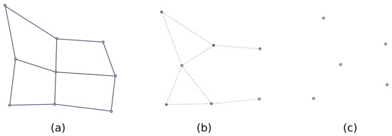
Figure 3.
An example of lattice structure of SOM (a), (G)NG (b) and K-means (c).
The lattice structure of the SOM, also known as the elastic net, adapts to the input data while trying to maintain its predefined topology. Thus, the “elastic net” has limited flexibility. However, given a sufficient number of BMUs or if the underlying manifold is 2D, the SOM can learn the topology of the manifold quite well. Whether the SOM represents the underlying manifold well can be measured by the so-called tophological error. This should not be confused with other measures of fitting quality; however, since it is by definition based on an unsupervised metric.
To put it formally: If M () denotes the manifold, the vectors of the manifold () can be described by a subset that we denote as (). The description of the data manifold via BMUs is considered optimal if the distortion (computed as e.g., ) is minimal. When Euclidean distance is used as a measure of distortion, the best matching units (BMUs) partition the manifold M into subregions corresponding to Voronoi polygons. Since each polygon is now described by a BMU, all vectors v within that polygon are represented by the vector . If the probability distribution of the data on the manifold M is described by the probability distribution , the average distortion (manifold reconstruction error) is determined by
and can be minimised by careful selection of .
When N is the number of data points on the manifold and , the distortion around becomes:
where is chosen w.r.t. . The optimal choice of for a given would be the representing the Voronoi polygon to which belongs. If we denote this Voronoi polygon by (as a class or “cluster”), we can rewrite the distortion (or loss) as follows:
It should now be apparent from this that both the Equations (2) and (4) can be used to minimise the distortion. However, other not-so-crisp update functions or other definitions of the neighbourhood can be used. For example, for a postsynaptic excitation we can choose a radial-basis function—typically a Gaussian—and define it for two neighbouring BMUs (namely i and k):
Here is just a parameter defining proximity. Now we can obtain the self-organising map (SOM) as defined by Kohonen, i.e.,:
This ends the explanation of the clustering methods used for the optimal selection of sensor locations. In the following subsections, the methods used for reconstruction and evaluation are explained.
3.4. K-Nearest Neighbours
The first method we will use to measure reconstruction error and evaluate the sensor location selection is based on proximity. We assume that the measurement at a particular location is best reconstructed based on the values near it, and that the contribution of each value to a final estimate is inversely proportional to distance. This can be simulated by using K-nearest neighbours (KNN) in a regression setting. In a regression setting, KNN can be observed as a variable bandwidth kernel-based estimator. If we use the Gaussian kernel and Euclidean distance, the estimated value is calculated as follows:
where is the distance between and in geographic space, k is the number of neighbours, N is the normalisation factor, and is given by:
Thus, is the average of the distances between the jth point and its k nearest neighbours. Since each value is reconstructed from k nearest neighbours, we have chosen .
3.5. Linear Regression
The second method we will use to measure reconstruction error and evaluate sensor location selection is based on linear regression. Linear regression assumes a relationship between the observed variable (v) and a set of n independent variables ():
where are the coefficients of the model we are trying to estimate to predict the value of the observed variable (v) given the independent variables (). Note that the complexity of the linear regression model increases as the number of available sensors increases. Since this is not the case for the KNN model, we might say that the comparison between them is somewhat unfair. However, we consider the diversity of the models as an advantage.
3.6. Reconstruction Error
To measure the reconstruction error of a vector field, we compared the estimated values with the true values at each location and time, and independently measured the amplitude error and the angular error. The amplitude error was calculated as the amplitude error averaged over the spatial and temporal dimensions:
where S and T denote the spatial and temporal axis, respectively, and and denote their cardinality (total number of elements).
Similarly, the angular error is the average angular error for each two vectors in time and space:
4. Results
4.1. Experimental Setup
The goal of the following experiments is to asses the quality of the reconstruction when different locations are used for data acquisition (sensor placement). Therefore, we investigate 3 different algorithms for location selection: K-means, GNG and SOM. The algorithms were used to sample data points in five cohorts, each with a different number of data points, namely: 10, 20, 50, 100, and 200, allowing us to conduct a total of 15 experiments for evaluation with linear regression and KNN.
The results are evaluated by calculating the reconstruction error as the error between the true and reconstructed values. The error is calculated as the mean and standard deviation for the angle and amplitude. Since we use learning models for reconstruction, it was necessary to split the data set into a training data set and a test data set. The dataset used was the data matrix containing u and v wind components of the data from the entire Mediterranean region. The data are organised as described in the previous section. The split was done in a ratio of 80:20, using the random 80% of realisations to train the models and leaving the rest for validation. After the learning process, the data of selected locations from the test set were used to reconstruct all other data from the test set.
While this approach will provide us the best sensor locations in terms of reconstruction error, in this work we did not aim to tackle solely this problem. In addition to providing a method for optimal sensor location selection in terms of reconstruction error, we are also investigating the possibility of selecting the optimal sensor location by introducing other criteria such as distance to shore, which are assumed to be related to deployment and maintenance costs. If this approach proves viable, it would suggest a more general framework since other variations are also possible. Therefore, we investigate the alternative in which the optimal sensor location is selected considering not only the distance to the cluster centre, but also the distance to the coast. In these experiments, each “optimal” point was updated towards the coast by using an additional term for the optimization criterion. The additional term can be considered as a regularisation term, which is a function of the distance to the shore. In our experiment, we weighted both terms equally.
Finally, to compare the results, random sensor locations were selected and reconstruction was performed based on the information provided by these locations.
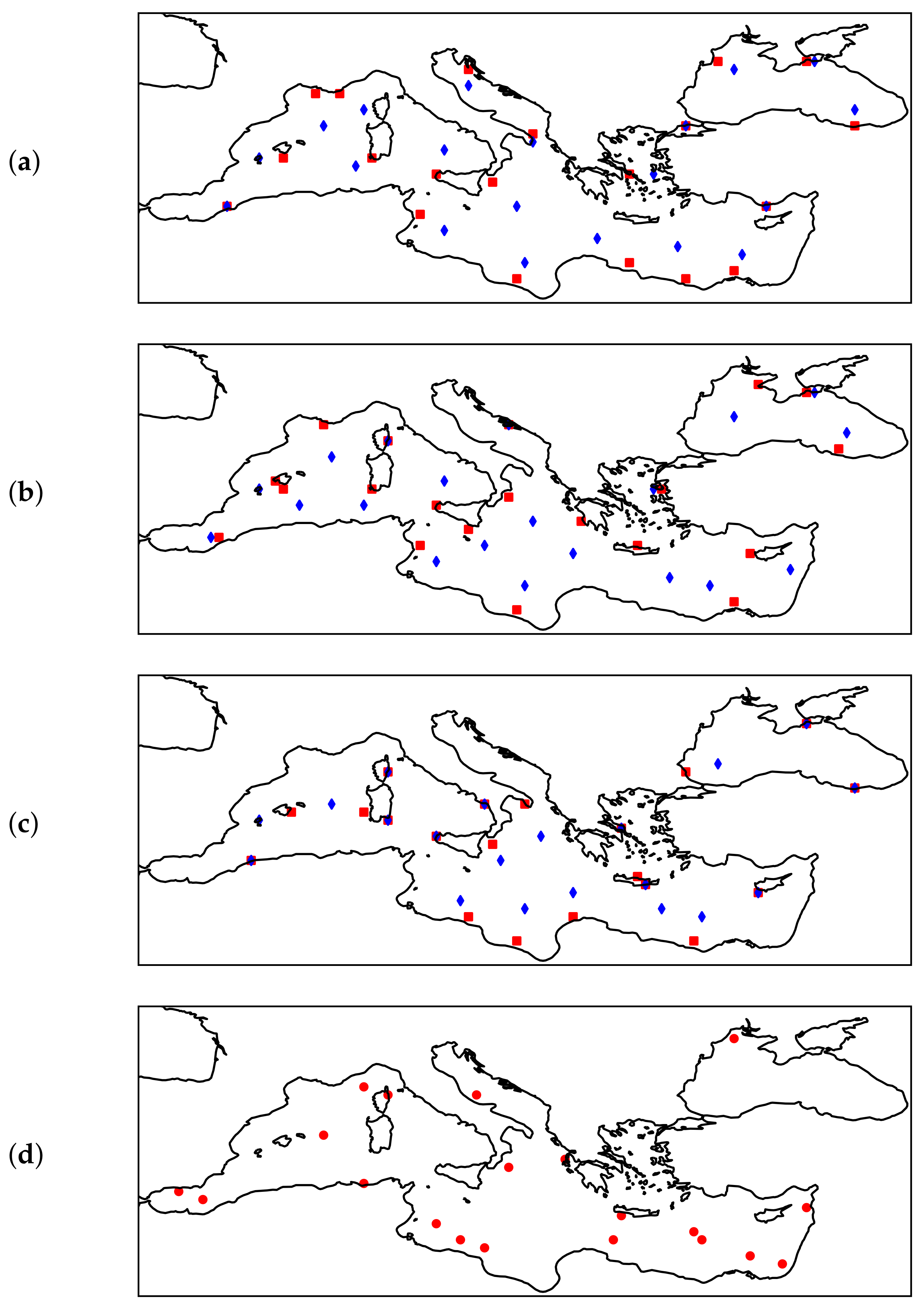
To get a better idea of how each algorithm (K-means, GNG, or SOM) selects the optimal sensor location for the standard and alternative approaches (where we also weighted the distance from shore), we visualised the results of these algorithms along with the results of the dummy algorithm that randomly selects sensor locations. This is shown in Figure 4 for a cohort of 20 sensor locations.
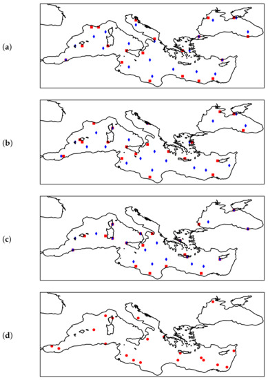
Figure 4.
From (a–d): Optimal sensor locations for 20 sensors determined by different algorithms. (a) K-means algorithm: blue—default, red—alternative implementation. (b) GNG algorithm: blue—default, red—alternative implementation. (c) SOM algorithm: blue—default, red—alternative implementation. (d) Dummy algorithm—random selection.
4.2. Experimenal Results
By default, regardless of which of the algorithms we use (K-means, GNG, or SOM), the optimal sensor location is selected as the data point closest to a cluster centre. These points were used to reconstruct sensor values for a much larger geographic area using linear regression and KNN. To assess the quality of the sensor location selection, we evaluate the quality of the reconstruction by measuring the difference between the true and reconstructed values. Since the measurements are 2D vectors, the error is described in terms of the mean amplitude and mean angle, and the standard deviation is given as a measure of the dispersion of the results. The results are presented in Table 1. The results can be compared with the data presented in Figure 1 which show the distribution of average wind data. The overall average wind amplitude is 5.55 m/s and the standard deviation is 3.05 m/s.

Table 1.
Table showing the reconstruction error measured as the average angular and amplitude error ( and ) and its standard deviation ( and ) for linear regression and KNN for sensor location selection using the k-menas, GNG, and SOM algorithms with default algorithm settings. Amplitude is given in m/s, angle in degrees.
From Table 1, we can see the reconstruction error when the optimal sensor location is selected as the data point closest to a cluster centre provided by one of the algorithms (K-means, GNG, or SOM). While the cluster centre is a sound option to obtain the representative data point in the following experiment, we also wanted to investigate how the reconstruction error behaves when other criteria contribute to the selection of the optimal sensor location. Therefore, in the following experiment, we simulated an alternative in which not only the distance to the cluster centre but also the distance to the shore is considered in the selection of the optimal sensor location. The results of this experiment are shown in Table 2.
Table 2.
Table showing the reconstruction error measured as the average angular and amplitude error ( and ) and its standard deviation ( and ) for linear regression and KNN for sensor location selection using the k-menas, GNG, and SOM algorithms with the additional criteria (alternative algorithm setting). The amplitude is given in m/s, the angle in degrees.
Finally, a random sample of the data is used to benchmark the results. This sample contained the same number of points as defined for each cohort, and reconstruction was performed using these points. The results are presented in Table 3.
Table 3.
Table showing reconstruction error measured as average angular and amplitude error ( and ) and its standard deviation ( and ) for linear regression and KNN with random selection of sensor locations (dummy algorithm). Amplitude is given in m/s, angle in degrees.
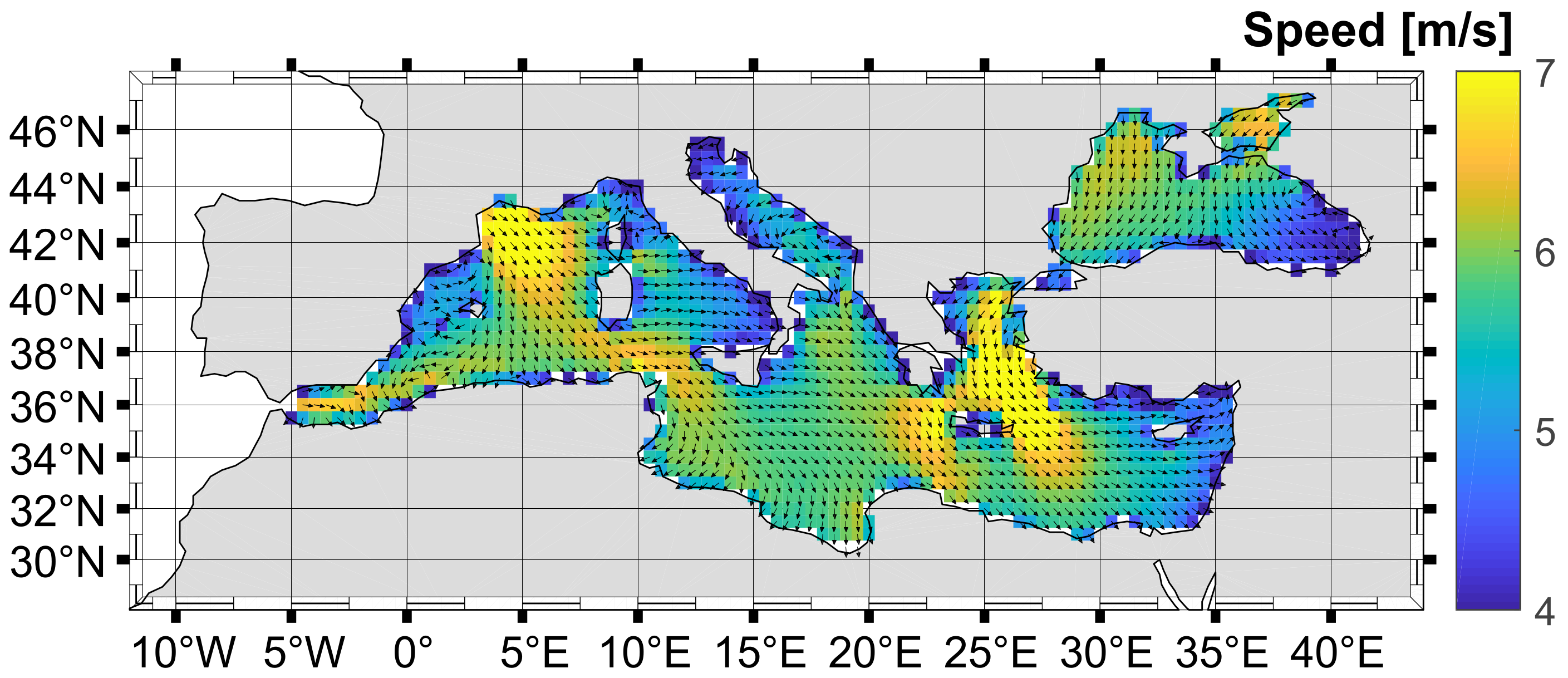
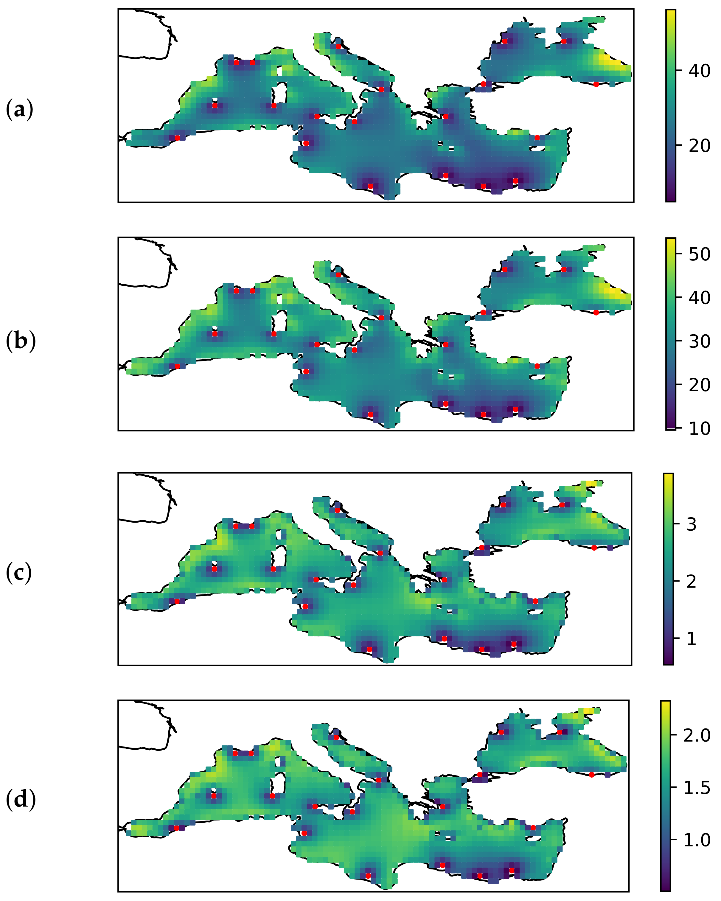
Figure 5 shows the spatial distribution of the error for the selection of 20 sensor locations using the K-means algorithm and distance to shore as an additional criterion. Thus, the sensor locations in this experiment correspond to the red squares in Figure 4a. The average amplitude and angular errors as well as the standard deviation can be found in Table 2.
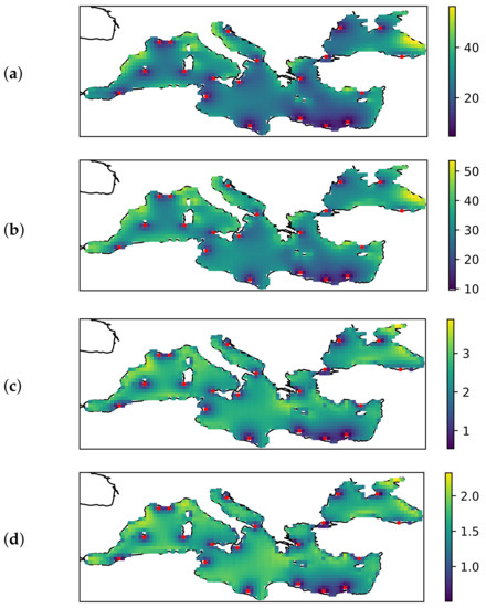
Figure 5.
From (a–d): spatial distribution of the error for the selection of 20 sensor location using the K-means algorithm and distance to shore as an additional criterion. (a) , (b) , (c) , (d) ; (a,b) are in degrees, (c,d) are in m/s. The red dots denote the optimal sensor location selected by this algorithm.
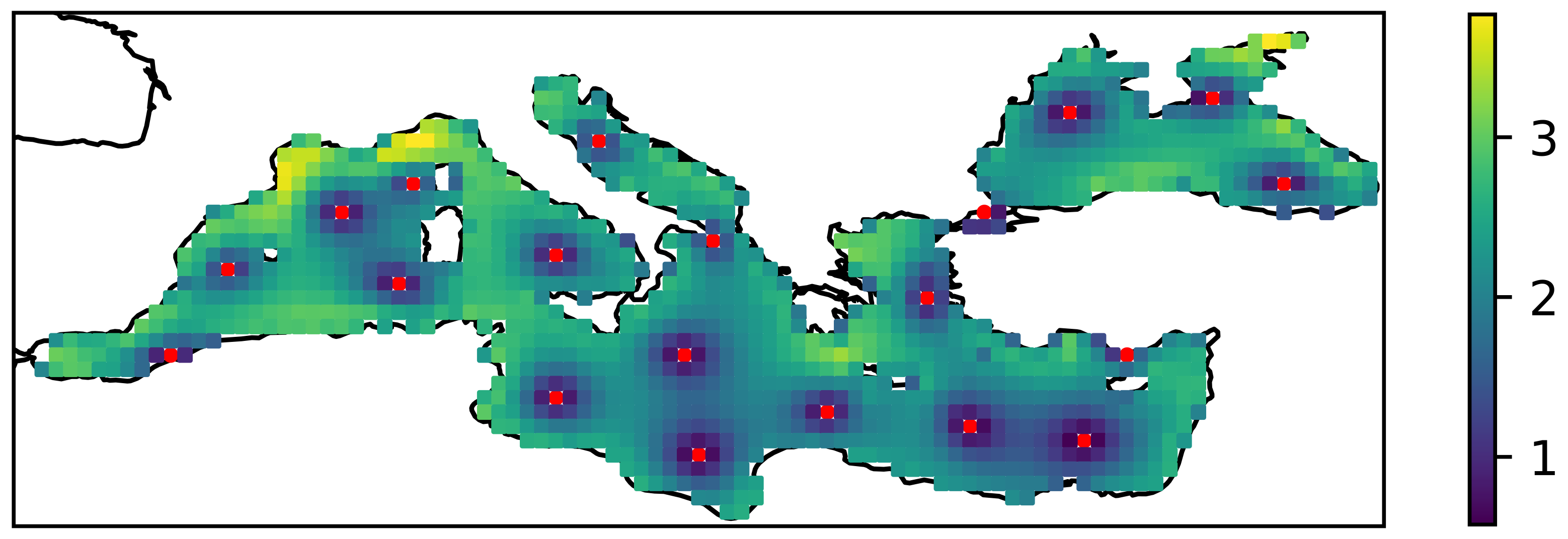
From Figure 5 it can be seen that the amplitude error increases rapidly as one moves away from sensor positions that are close to the coast. A similar effect is observed when the default algorithm is used, i.e., when distance to cost is not considered. Figure 6 shows the spatial distribution of the error for the optimal selection for a case with 20 sensors. It can be seen that the error increases as one moves away from the sensor location, even if the sensor is in the open sea—but perhaps less rapidly.
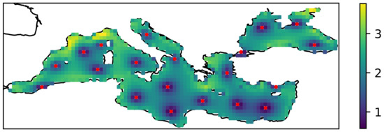
Figure 6.
Spatial distribution of amplitude error () for the selection of 20 sensor location. The red dots denote the optimal sensor location selected by the algorithm that does not take into account the distance to shore.
5. Discussion
In our first experiment, the results of which are shown in Table 1, we have shown that a small number of points is sufficient to reconstruct measurements from a larger geographical area quite accurately. This corroborates the results presented in [18,19]. While previous works have discussed the reconstruction error over the Adriatic, we show here that similar conclusions hold when wind data are used over the Mediterranean. The larger overall error could be due not only to the larger geographical area observed in the study, but also to the larger amplitude variance of the wind, which can reach 50 m/s in the case of the Mediterranean Sea. When we compare the results from Table 1 and Table 3, we conclude that an optimal sensor location can be intelligently selected and that—compared to other proposed algorithms—the K-means algorithm gives the best results. Furthermore, if we want to choose between KNN and linear regression as a method for reconstructing wind data over the Mediterranean Sea, the Table 1, Table 2 and Table 3 suggest that KNN is more suitable than linear regression for this purpose if we are to reconstruct data from a small number of sensors. On the other hand, if a larger number of sensors (>20) is used, linear regression is superior to KNN in terms of reconstruction error. This can be attributed to the fact that the complexity of a linear regression model increases with the number of available sensors, while the KNN model stays with a fixed set of parameters.
However, this work had a more ambitious goal than this. We aimed to show that a more general framework for optimal sensor site selection is possible using this approach. To show that other criteria can be used in selecting the optimal sensor location, we introduced distance to shore, which is presumed to be related to deployment and maintenance costs. This change shows that other variations are possible and that an optimal sensor location can be selected using a different criterion for the optimum if a tradeoff between, e.g., accuracy and cost is an option. When the criterion is weighted with respect to distance from the coast, so that the representative data points are selected not as the data points closest to the cluster centre but as the representative data points near the coast, we obtain the results shown in Table 2.
Comparing the results from Table 1, Table 2 and Table 3, we see that the best results (in terms of reconstruction error) for the standard experimental setup are obtained when the optimal sensor position does not consider the distance to the shore. However, when the distance to the shore is taken into account, the results deteriorate, and this deterioration can reach for a smaller number of sensor locations (10, 20 or 50), which are probably of our main interest. It is also worth noting that the optimal sensor location selection algorithm plays a less significant role when the distance to shore is included in the search for the optimal sensor location. This should correspond to the common sense, since this additional criterion is common to all algorithms and thus practically cancels the differences.
When we compare the results of the first two experiments (Table 1 and Table 2) with the random selection of sensor locations (results from Table 3), we find that the random selection additionally degrades the performance of the reconstruction algorithms. As expected, this degradation is smaller when a larger number of sensor locations are selected. It is worth noting that compared to Table 2, random site selection (Table 3) gives better results for the experiment with a larger number of sensor sites (e.g., 200). This is easily explained by the fact that the results in Table 2 were obtained with the additional constraint that the sites were selected near the shore, which was not the case with random selection. To illustrate the importance of this constraint, note that when we select sensor sites that are less than 1 px (which is about 31 km) from the shore, we select 200 sensor sites out of 372 available sites.
Other specifics that are not obvious from the tables, but still worth mentioning, can be seen in Figure 4 and Figure 5. From Figure 5 we can see how the error (and variability) increases as we move further away from the sensor. However, from the figure, we can also see how the sensors on the North African coast are used to capture variability in the Aegean Sea, and how the Crimean Peninsula is important to capture variability in the Black Sea. From an oceanographic perspective, this is partly due to the strong and dominant winds in these areas. In addition, not one, but two sensor sites were selected for the Gulf of Lion which can be attributed to the strong mistral winds and their variability.
It is also clear from Figure 5 that some parts of the Mediterranean Sea are selected by all three algorithms for optimal sensor placement. These locations include the Black Sea (especially the western part), the Ligurian Sea, and the Aegean Sea. We hypothesise that this is due to the large amount of energy that accumulates in these regions, or the large wind variability in certain spatial and temporal regions. For example, the wind over the Black Sea is independent of the wind in the other areas examined in this study. Similarly, the sensors south of Crete record quasi-permanent W/NW winds over most of the eastern Mediterranean, so they are only weakly correlated with other areas in the Mediterranean. On the other hand, sensors in the Ligurian Sea are associated with an extremely strong wind pattern generated by a mesoscale cyclone.
Perhaps it is also worth noting that when a smaller number of sensors are selected, some effects are neglected by certain algorithms. This is especially true for the Adriatic Sea, for which SOM and GNG do not select a sensor location when only 20 sensors are selected, as shown in Figure 4. With a smaller number of sensors, this difference between the sensors selected by K-means and SOM is also observed in the Black Sea. From a geophysical point of view, it is interesting to note that the K-means algorithm gives the best result and that this is due to the fundamental differences between the algorithms. For certain geophysical problems, topology preservation seems to be more of a nuisance than an advantage. As mentioned earlier, the topology preservation property may have as a side effect that some of the data variability is not accounted for.
6. Conclusions
In this work, we have shown that optimal sensor locations can be intelligently selected using data-oriented unsupervised learning methods such as K-means, NG, and SOM. The case study conducted with wind data from the Mediterranean region showed that the K-means algorithm gave the best results compared to the other proposed algorithms (cf. Table 1, Table 2 and Table 3). Moreover, the tables suggest that KNN is more suitable than linear regression for this purpose when the data are reconstructed from a small number of sensors. On the other hand, when a larger number of sensors (>20) are used, linear regression is superior to KNN in terms of reconstruction error.
Next, we showed that this approach can be used as a general framework for optimal sensor placement and that other criteria can be incorporated into the selection of the optimal sensor location. To do this, we extended our case study to include distance to shore, which is believed to be related to deployment and maintenance costs. This demonstration not only showed that the inclusion of additional criteria significantly affects the results in terms of sensor location (Figure 4) and reconstruction accuracy (Table 2), but also provided a more general framework in which other variations are possible, such that the optimal sensor location can be selected using a different criterion for the optimum if a tradeoff between, for example, e.g., accuracy and cost is an option.
Finally, we conclude that the work corroborates previous results showing that a small number of points is sufficient to reconstruct measurements from a larger geographic area such as the Mediterranean. Only a small fraction of the data (10 points) is sufficient to achieve an error of less than 3 m/s, which is comparable to the error of meteorological models for the same geographical area. Furthermore, we have proposed a broader framework in which clustering algorithms are used for optimal sensor placement and that, if desired, a tradeoff between e.g., accuracy and measurement cost can be implemented in addition to these algorithms. While this tradeoff degrades reconstruction accuracy, it also provides the opportunity to use a more complex model to achieve better reconstruction. In addition to using more advanced machine learning models, one research direction that could further reduce the number of sensors or increase accuracy is assimilation of sensor data coupled with fine physical models. Fine physical models have this potential but tend to be more time-consuming.
Author Contributions
Conceptualization, H.K.; methodology, H.K.; software, H.K., L.Ć.; validation, H.K.; formal analysis, H.K.; writing—original draft preparation, H.K.; writing—review and editing, H.K., F.M.; visualization, H.K., F.M.; supervision, H.K.; project administration, H.K.; funding acquisition, H.K. All authors have read and agreed to the published version of the manuscript.
Funding
This work has been supported in part by Croatian Science Foundation under the project UIP-2019-04-1737.
Data Availability Statement
Data used in this study are available in a publicly accessible repository Copernicus Climate Change Service at https://doi.org/10.24381/cds.adbb2d47.
Conflicts of Interest
The authors declare no conflict of interest. The funders had no role in the design of the study; in the collection, analyses, or interpretation of data; in the writing of the manuscript, or in the decision to publish the results.
Abbreviations
The following abbreviations are used in this manuscript:
| ECMWF | European Center for Medium-range Weather Forecasts |
| SOM | Self-organizing map |
| GNG | Growing neural gas |
| BMU | Best matching unit |
| KNN | K-nearest neighbours |
References
- Jaimes, A.; Tweedie, C.; Magoč, T.; Kreinovich, V.; Ceberio, M. Optimal Sensor Placement in Environmental Research: Designing a Sensor Network under Uncertainty. In Proceedings of the 4th International Workshop on Reliable Engineering Computing REC’2010, Singapore, 3–5 March 2010; pp. 255–267. [Google Scholar]
- Joshi, S.; Boyd, S. Sensor Selection via Convex Optimization. IEEE Trans. Signal Process. 2009, 57, 451–462. [Google Scholar] [CrossRef] [Green Version]
- Chiu, P.; Lin, F. A simulated annealing algorithm to support the sensor placement for target location. In Proceedings of the Canadian Conference on Electrical and Computer Engineering 2004, Niagara Falls, ON, Canada, 2–5 May 2004; Volume 2, pp. 867–870. [Google Scholar] [CrossRef]
- Zhao, Z.; He, X.; Cai, D.; Zhang, L.; Ng, W.; Zhuang, Y. Graph Regularized Feature Selection with Data Reconstruction. IEEE Trans. Knowl. Data Eng. 2016, 28, 689–700. [Google Scholar] [CrossRef]
- Farahat, A.K.; Ghodsi, A.; Kamel, M.S. An Efficient Greedy Method for Unsupervised Feature Selection. In Proceedings of the 2011 IEEE 11th International Conference on Data Mining, Vancouver, BC, Canada, 11–14 December 2011; pp. 161–170. [Google Scholar] [CrossRef]
- Masaeli, M.; Fung, G.; Dy, J.G. Convex principal feature selection. In Proceedings of the 2010 SIAM International Conference on Data Mining, Columbus, OH, USA, 29 April–1 May 2010; pp. 619–628. [Google Scholar]
- Zheng, Z.; Ma, H.; Yan, W.; Liu, H.; Yang, Z. Training Data Selection and Optimal Sensor Placement for Deep-Learning-Based Sparse Inertial Sensor Human Posture Reconstruction. Entropy 2021, 23, 588. [Google Scholar] [CrossRef] [PubMed]
- Aghazadeh, A.; Golbabaee, M.; Lan, A.; Baraniuk, R. Insense: Incoherent sensor selection for sparse signals. Signal Process. 2018, 150, 57–65. [Google Scholar] [CrossRef] [Green Version]
- Rao, S.; Chepuri, S.P.; Leus, G. Greedy Sensor Selection for Non-Linear Models. In Proceedings of the 2015 IEEE 6th International Workshop on Computational Advances in Multi-Sensor Adaptive Processing (CAMSAP), Cancun, Mexico, 13–16 December 2015; pp. 241–244. [Google Scholar]
- Ranieri, J.; Chebira, A.; Vetterli, M. Near-Optimal Sensor Placement for Linear Inverse Problems. IEEE Trans. Signal Process. 2014, 62, 1135–1146. [Google Scholar] [CrossRef] [Green Version]
- Guestrin, C.; Krause, A.; Singh, A.P. Near-optimal sensor placements in gaussian processes. In Proceedings of the 22nd International Conference on Machine Learning, Bonn, Germany, 7–11 August 2005. [Google Scholar]
- Naeem, M.; Xue, S.; Lee, D. Cross-Entropy optimization for sensor selection problems. In Proceedings of the 9th International Symposium on Communications and Information Technology, Icheon, Korea, 28–30 September 2009. [Google Scholar] [CrossRef]
- Wang, H.; Yao, K.; Pottie, G.; Estrin, D. Entropy-Based Sensor Selection Heuristic for Target Localization. In Proceedings of the 3rd International Symposium on Information Processing in Sensor Networks, Berkeley, CA, USA, 26–27 April 2004; pp. 36–45. [Google Scholar] [CrossRef] [Green Version]
- Cai, D.; Zhang, C.; He, X. Unsupervised Feature Selection for Multi-Cluster Data. In Proceedings of the 16th ACM SIGKDD International Conference on Knowledge Discovery and Data Mining, Washington, DC, USA, 24–28 July 2010; pp. 333–342. [Google Scholar] [CrossRef] [Green Version]
- Chandrashekar, G.; Sahin, F. A survey on feature selection methods. Comput. Electr. Eng. 2014, 40, 16–28. [Google Scholar] [CrossRef]
- Gao, S.; Ver Steeg, G.; Galstyan, A. Variational Information Maximization for Feature Selection. In Advances in Neural Information Processing Systems; Lee, D., Sugiyama, M., Luxburg, U., Guyon, I., Garnett, R., Eds.; Curran Associates, Inc.: Red Hook, NY, USA, 2016; Volume 29. [Google Scholar]
- Roy, D.; Murty, K.S.R.; Mohan, C.K. Feature selection using Deep Neural Networks. In Proceedings of the 2015 International Joint Conference on Neural Networks (IJCNN), Killarney, Ireland, 12–17 July 2015; pp. 1–6. [Google Scholar] [CrossRef]
- Kalinić, H.; Bilokapić, Z.; Matić, F. Can Local Geographically Restricted Measurements Be Used to Recover Missing Geo-Spatial Data? Sensors 2021, 21, 3507. [Google Scholar] [CrossRef] [PubMed]
- Kalinić, H.; Bilokapić, Z.; Matić, F. Oceanographic data reconstruction using machine learning techniques. In Proceedings of the EGU General Assembly 2021, Online, 19–30 April 2021. [Google Scholar] [CrossRef]
- Duda, R.O.; Hart, P.E.; Stork, D.G. Pattern Classification, 2nd ed.; John Wiley & Sons, Inc.: New York, NY, USA, 2001. [Google Scholar]
- Kohonen, T. Self-organized formation of topologically correct feature maps. Biol. Cybern. 1982, 43, 59–69. [Google Scholar] [CrossRef]
- Kohonen, T.; Huang, T.; Schroeder, M. Self-Organizing Maps; Physics and Astronomy Online Library, Springer: Berlin/Heidelberg, Germany, 2001. [Google Scholar]
- Martinetz, T.; Berkovich, S.; Schulten, K. “Neural-Gas” Network for Vector Quantization and its Application to Time-Series Prediction. IEEE Trans. Neural Netw. 1993, 4, 558–569. [Google Scholar] [CrossRef] [PubMed]
- Fritzke, B. A Growing Neural Gas Network Learns Topologies. In Advances in Neural Information Processing Systems; Tesauro, G., Touretzky, D., Leen, T., Eds.; MIT Press: Denver, CO, USA, 1994; Volume 7. [Google Scholar]
- Jain, A.K. Data clustering: 50 years beyond K-means. Pattern Recognit. Lett. 2010, 31, 651–666. [Google Scholar] [CrossRef]
- Šantić, D.; Piwosz, K.; Matić, F.; Vrdoljak Tomaš, A.; Arapov, J.; Dean, J.L.; Šolić, M.; Koblížek, M.; Kušpilić, G.; Šestanović, S. Artificial neural network analysis of microbial diversity in the central and southern Adriatic Sea. Sci. Rep. 2021, 11, 11186. [Google Scholar] [CrossRef] [PubMed]
- Solidoro, C.; Bandelj, V.; Barbieri, P.; Cossarini, G.; Fonda Umani, S. Understanding dynamic of biogeochemical properties in the northern Adriatic Sea by using self-organizing maps and k-means clustering. J. Geophys. Res. Ocean. 2007, 112, C07S90. [Google Scholar] [CrossRef] [Green Version]
- Šolić, M.; Grbec, B.; Matić, F.; Šantić, D.; Šestanović, S.; Ninčević Gladan, Ž.; Bojanić, N.; Ordulj, M.; Jozić, S.; Vrdoljak, A. Spatio-temporal reproducibility of the microbial food web structure associated with the change in temperature: Long-term observations in the Adriatic Sea. Prog. Oceanogr. 2018, 161, 87–101. [Google Scholar] [CrossRef]
- Matić, F.; Kalinić, H.; Vilibić, I.; Grbec, B.; Morožin, K. Adriatic-Ionian air temperature and precipitation patterns derived from self-organizing maps: Relation to hemispheric indices. Clim. Res. 2019, 78, 149–163. [Google Scholar] [CrossRef]
- Ninčević Gladan, Ž.; Matić, F.; Arapov, J.; Skejić, S.; Bužančić, M.; Bakrač, A.; Straka, M.; Dekneudt, Q.; Grbec, B.; Garber, R.; et al. The relationship between toxic phytoplankton species occurrence and environmental and meteorological factors along the Eastern Adriatic coast. Harmful Algae 2020, 92, 101745. [Google Scholar] [CrossRef] [PubMed]
- Durán, P.; Basu, S.; Meißner, C.; Adaramola, M.S. Automated classification of simulated wind field patterns from multiphysics ensemble forecasts. Wind Energy 2020, 23, 898–914. [Google Scholar] [CrossRef]
- Ohba, M. The Impact of Global Warming on Wind Energy Resources and Ramp Events in Japan. Atmosphere 2019, 10, 265. [Google Scholar] [CrossRef] [Green Version]
- Berkovic, S. Winter Wind Regimes over Israel Using Self-Organizing Maps. J. Appl. Meteorol. Climatol. 2017, 56, 2671–2691. [Google Scholar] [CrossRef]
- Kalinić, H.; Mihanović, H.; Cosoli, S.; Tudor, M.; Vilibić, I. Predicting ocean surface currents using numerical weather prediction model and Kohonen neural network: A northern Adriatic study. Neural Comput. Appl. 2017, 28, 611–620. [Google Scholar] [CrossRef]
- Vilibić, I.; Šepić, J.; Mihanović, H.; Kalinić, H.; Cosoli, S.; Janeković, I.; Žagar, N.; Jesenko, B.; Tudor, M.; Dadić, V.; et al. Self-Organizing Maps-based ocean currents forecasting system. Sci. Rep. 2016, 6, 22924. [Google Scholar] [CrossRef] [PubMed]
- Hersbach, H.; Bell, B.; Berrisford, P.; Biavati, G.; Horányi, A.; Muñoz Sabater, J.; Nicolas, J.; Peubey, C.; Radu, R.; Rozum, I.; et al. ERA5 Hourly Data on Single Levels from 1959 to Present. Copernicus Climate Change Service (C3S) Climate Data Store (CDS). 2018. Available online: https://cds.climate.copernicus.eu/cdsapp#!/dataset/reanalysis-era5-single-levels?tab=overview (accessed on 16 June 2022).
Publisher’s Note: MDPI stays neutral with regard to jurisdictional claims in published maps and institutional affiliations. |
© 2022 by the authors. Licensee MDPI, Basel, Switzerland. This article is an open access article distributed under the terms and conditions of the Creative Commons Attribution (CC BY) license (https://creativecommons.org/licenses/by/4.0/).