Assessment of Machine Learning Techniques for Oil Rig Classification in C-Band SAR Images

Abstract

This article aims at performing maritime target classification in SAR images using machine learning (ML) and deep learning (DL) techniques. In particular, the targets of interest are oil platforms and ships located in the Campos Basin, Brazil. Two convolutional neural networks (CNNs), VGG-16 and VGG-19, were used for attribute extraction. The logistic regression (LR), random forest (RF), support vector machine (SVM), k-nearest neighbours (kNN), decision tree (DT), naive Bayes (NB), neural networks (NET), and AdaBoost (ADBST) schemes were considered for classification. The target classification methods were evaluated using polarimetric images obtained from the C-band synthetic aperture radar (SAR) system Sentinel-1. Classifiers are assessed by the accuracy indicator. The LR, SVM, NET, and stacking results indicate better performance, with accuracy ranging from 84.1% to 85.5%. The Kruskal–Wallis test shows a significant difference with the tested classifier, indicating that some classifiers present different accuracy results. The optimizations provide results with more significant accuracy gains, making them competitive with those shown in the literature. There is no exact combination of methods for SAR image classification that will always guarantee the best accuracy. The optimizations performed in this article were for the specific data set of the Campos Basin, and results may change depending on the data set format and the number of images.

1. Introduction

The seas and oceans are natural resources of oil, natural gas, fauna, and flora, rich in biodiversity and ecosystems. Because of those attributes, the Brazilian marine area is known as the “Blue Amazon” [1]. The Campos Basin, one of the largest oil and gas producers in Brazil, is located on the northern coast of Rio de Janeiro, between the cities of Vitória (ES) and Cabo Frio (RJ), covering an area of 120,000 km² [2].

The production capacity of oil and natural gas at sea can be evidenced by the results for July 2021 in the Monthly Bulletin number 131 [3], highlighting the Campos and Santos basins. For this period, the offshore oil and natural gas production was at about 97.1% and 82.5% capacity, respectively [3]. In particular, the Campos and Santos Basins were responsible for 23.74% and 69.07% of national oil and natural gas production, respectively. Consequently, the sea is of strategic importance to the Brazilian economy. Its constant surveillance is necessary to avoid illegal exploitation, such as fishing, oil spills, maritime traffic, and piracy [4].

Remote sensing allows the surveillance of large maritime areas [5]. The US Seasat mission provided the first earth-imaging synthetic aperture radar (SAR) from space, launched in 1978. The European Space Agency developed and launched the first microwave SAR systems, ERS-1 (launched on 17 July 1991) and ERS-2 (launched on 20 April 1995) [6]. SAR systems have been applied in earth remote sensing applications for more than 30 years due to their ability to provide high-resolution images, independent of the weather conditions and sunlight illumination [7]. Furthermore, SAR images play an important role in maritime surveillance [8,9], being useful for civil and military applications [10], such as detecting environmental accidents related to oil spills [11,12].

SAR images can be difficult to interpret with human vision. To overcome this limitation, automatic target recognition (ATR) can be applied to extract features that contain unique identifying information about the targets. ATR consists of three stages, known as detection, recognition, and classification [13]. This article will focus on the classification step [14], and more precisely, on the classification of two types of targets, oil rigs and ships.

Recently, artificial intelligence (AI) techniques such as machine learning (ML) [15] and deep learning (DL) [13] have been widely used for target classification in different SAR image applications [16,17,18]. As discussed in [16], a hybrid neural network was employed in Sentinel-1 and RADARSAT-2 SAR images for classification purposes. The hybrid algorithm consisted of a convolutional neural network (CNN) and a multilayer perceptron (MLP). As a result, the classification performance increased. ML is a subset area of AI that enables computer systems to learn from past experiences and improve their behavior for specific tasks. Typical examples of ML schemes are support vector machines (SVM), decision tree (DT), naive Bayes (NB), and k-means clustering [19,20]. Neural networks (NET) are a subset of ML inspired by biological neural networks, being represented by artificial neurons connected in layers [20,21], while DL is an NET technique that organizes neurons into several layers [20,22], for example, deep neural network (DNN) and CNN [20]. DL has become popular in object detection due to its ability to learn how to discriminate features automatically [23]. Furthermore, ML techniques, such as logistic regression (LR) and NET, have shown to be useful for oil slick detection in SAR images from Sentinel-1 orbital systems [11]. For instance, in [24], a CNN was used to increase the training and test data sets in ship detection in Gaofen-3 SAR images. A SAR ATR CNN-based application was performed with the public MSTAR data set in [25] to classify military vehicles in SAR images, displaying competitive results with the literature in terms of accuracy.

This article compares ML techniques, such as random forest (RF), LR, NET, SVM, AdaBoost (ADBST), k-nearest-neighbours (kNN), NB, and DT, for classifying maritime targets in high-resolution SAR images. For attribute extraction, two visual geometry group deep learning techniques (VGG-16 and VGG-19) are considered. In particular, we aim to classify oil rigs and ships in the Campos Basin, on the coast of Rio de Janeiro and Espírito Santo, Brazil, considering vertical-horizontal (VH) and vertical-vertical (VV) polarimetric images. For that, we considered the following methods: (M1) reproduction of results already presented in the literature, specifically the ones discussed in [26], which, to the best of our knowledge, is the only study related to the Campos Basin data set; (M2) evaluation of the sensitivity of the classifiers; (M3) expansion of the training data set concatenation considering the whole of the VH and VV polarization samples; (M4) expansion of the training data set concatenating half of the VH and VV polarization samples; and (M5) combining classifiers to obtain better accuracy results (a technique named stacked generalization).

To achieve this objective, the aims of this article are as follows:

(i)

Evaluate the combination of machine learning methods associated with classification with deep learning for feature extraction;

(ii)

Evaluate ML methods in the classification of SAR images in the C-Band and DL for attribute extraction;

(iii)

Reproduce the results of [26] to validate the methodology;

(iv)

Identify parameter adjustments with more significant gains than those achieved in the literature;

(v)

Combine data sets to increase the variability of training samples;

(vi)

Combine classification techniques;

(vii)

Analyze the performance of VGG-16 and VGG-19 networks as feature generators for classification algorithms;

(viii)

Evaluate the significance of the results through non-parametric statistics.

The remainder of the paper is organized as follows. Section 2.1 presents the Sentinel-1 mission and the employed data set. In Section 2.2, the used classification tools are presented. The classification setup applied in this study is described in Section 2.3. The numerical analyses are included in Section 3. Finally, Section 4 concludes the paper.

2. Materials and Methods

This section presents the characteristics of the Sentinel-1 mission, the classification techniques, and the methodology used in this article.

2.1. Sentinel-1 Mission

The data set employed in this studied was obtained through the Sentinel-1 mission, which is composed of two satellites, namely Sentinel-1A and Sentinel-1B, launched in 3 April 2014 and 25 April 2016, respectively [27]. They are in a sun-synchronized near-polar orbit, operating day and night, with a 12-day repetition cycle and an altitude of 693 km, and they perform C-band SAR imaging [28,29]. This satellite has an SAR sensor capable of generating medium- and high-resolution measurements [28]. In

Table 1. Summary of the Sentinel-1 system parameters and characteristics.

Name	Sentinel-1
Band	C
Bandwidth	0–100 MHz (programmable)
Centre frequency	5.405 GHz
Storage capacity	1410 Gb
Polarization	HH+HV, VV+VH
	VV, HH
Incidence angle range	20–46°
Look direction	right
Antenna type	Slotted wave-guide radiators
Antenna size	12.3 m × 0.821 m
Antenna mass	880 kg
Azimuth beam width	0.23°
PRF (pulse repetition frequency)	1–3 kHz (programmable)
Data quantization	10 bit
Total instrument mass (including antenna)	945 kg

Font: [27].

, some of the Sentinel-1 system characteristics, such as the operating band, bandwidth, antenna size, antenna weight, and pulse repetition frequency, are presented [27]. The Sentinel-1 systems support single- (HH or VV) and dual-polarization (HH + HV or VV + VH) operations, implemented by a transmit chain (switchable between H or V) and two parallel receive chains for H and V polarization. Additionally, the stripmap (SM), interferometric wide swath (IW), and extra-wide swath (EW) products are available with single or dual-polarization. However, the waver product is only available with single polarization [27].

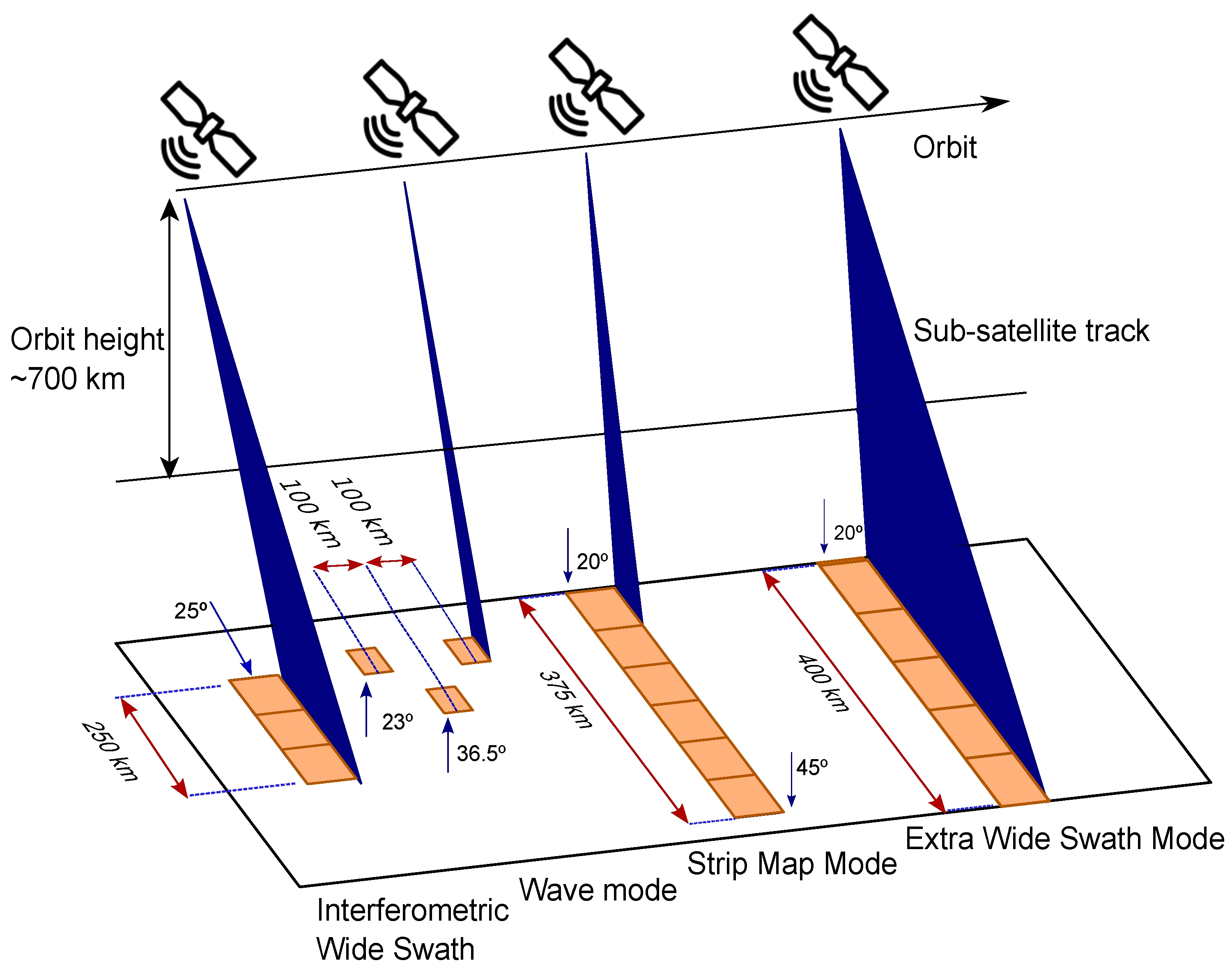
According to [27], Sentinel-1 can acquire data in four modes, which are described in the following and shown in Figure 1. First, SM is a standard SAR stripmap imaging mode. A continuous sequence of pulses with a fixed elevation angle illuminates a strip of ground. Second, in IW mode, the data are acquired in three bands using the terrain observation with progressive scanning SAR (TOPSAR) imaging technique. Third, the data are acquired on five swaths using the TOPSAR imaging technique. The EW mode provides extensive swath coverage at the expense of spatial resolution. Finally, in WV mode, the data are obtained in small stripmap scenes called “vignettes”, located at regular $100\mathrm{km}$ intervals along the swath.

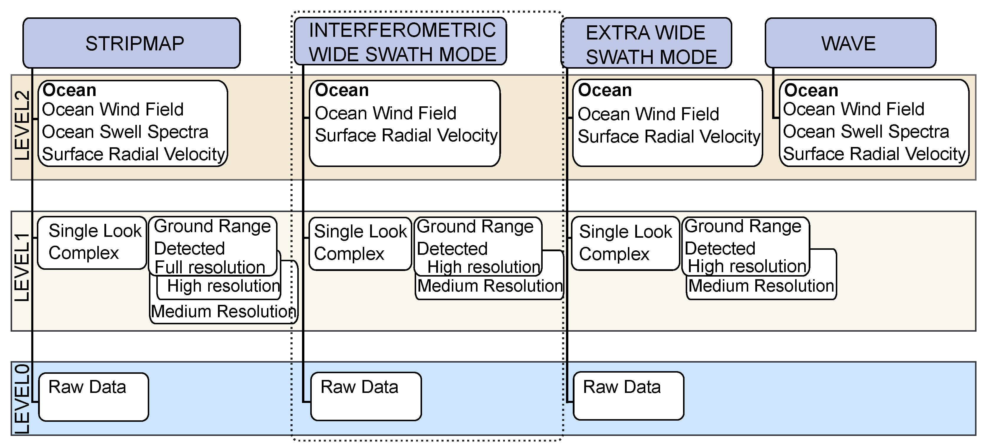
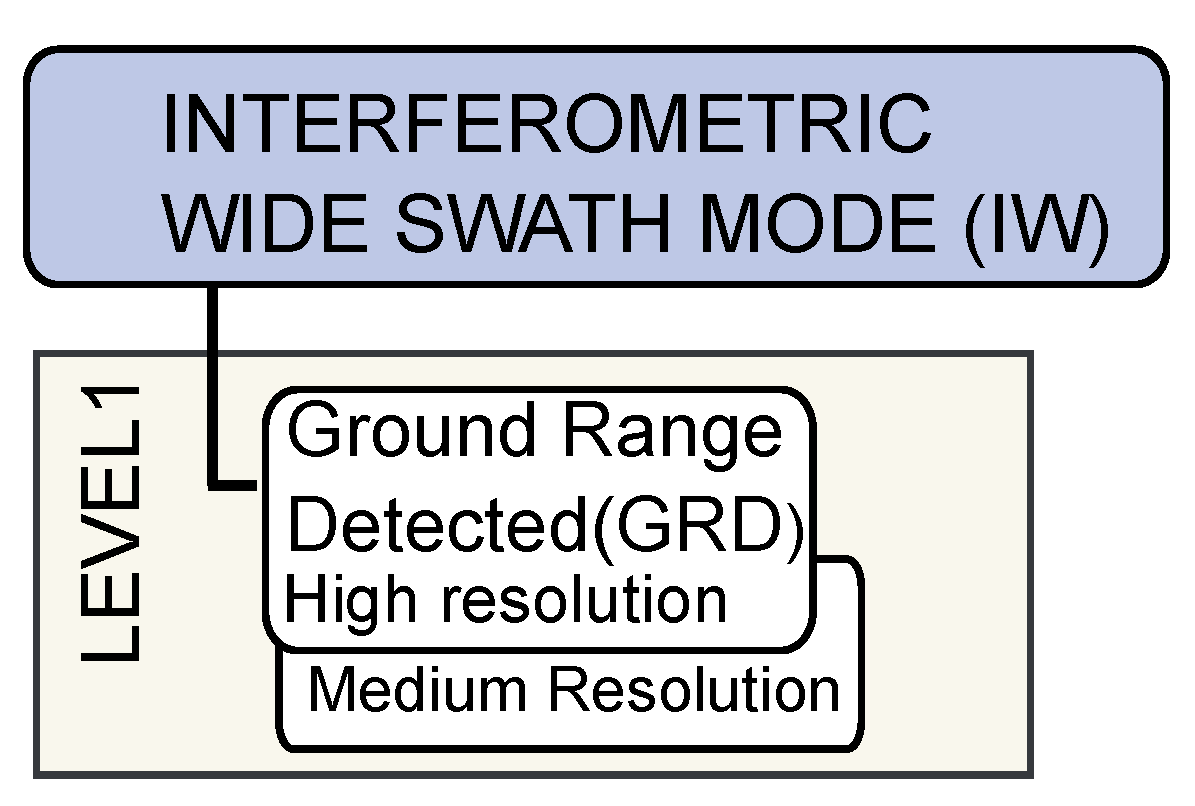
The four acquisition modes (SM, IW, EW, WV) can generate SAR level 0, level 1 SLC, level 1 GRD, and level 2 OCN products [27], as shown in Figure 2. The product used in our research is level 1 GRD with high-resolution SAR images, in IW mode, as shown in Figure 3. It consists of focused SAR data detected, multi-looked, and projected to the ground range using an ellipsoid model.

Table 2. Typical Sentinel-1 applications distributed by modes.

Application	Mode
	SM	IW	EW	WV
Arctic and sea-ice		X	X
Open ocean ship surveillance		X	X
Oil pollution monitoring		X	X
Marine winds		X	X	X
Forestry		X
Agriculture		X
Urban deformation mapping		X
Flood monitoring	X	X
Earthquake analysis	X	X
Landslide and volcano monitoring	X	X

shows some examples of applications separated by operating modes.

Sentinel-1 Image Data Set

For this study, the Sentinel-1 SAR image data set contains 400 images (patches) in VH and VV polarization with maritime targets (platforms and ships), equally distributed (i.e., 200 patches with platforms and 200 patches with ships). Image patches were acquired at different times. There are targets with more than one patch. Despite being from the same target, the patches can be considered distinct because of the SAR image formation process, which is influenced by backscatter and sea currents that cause displacement on the platforms.

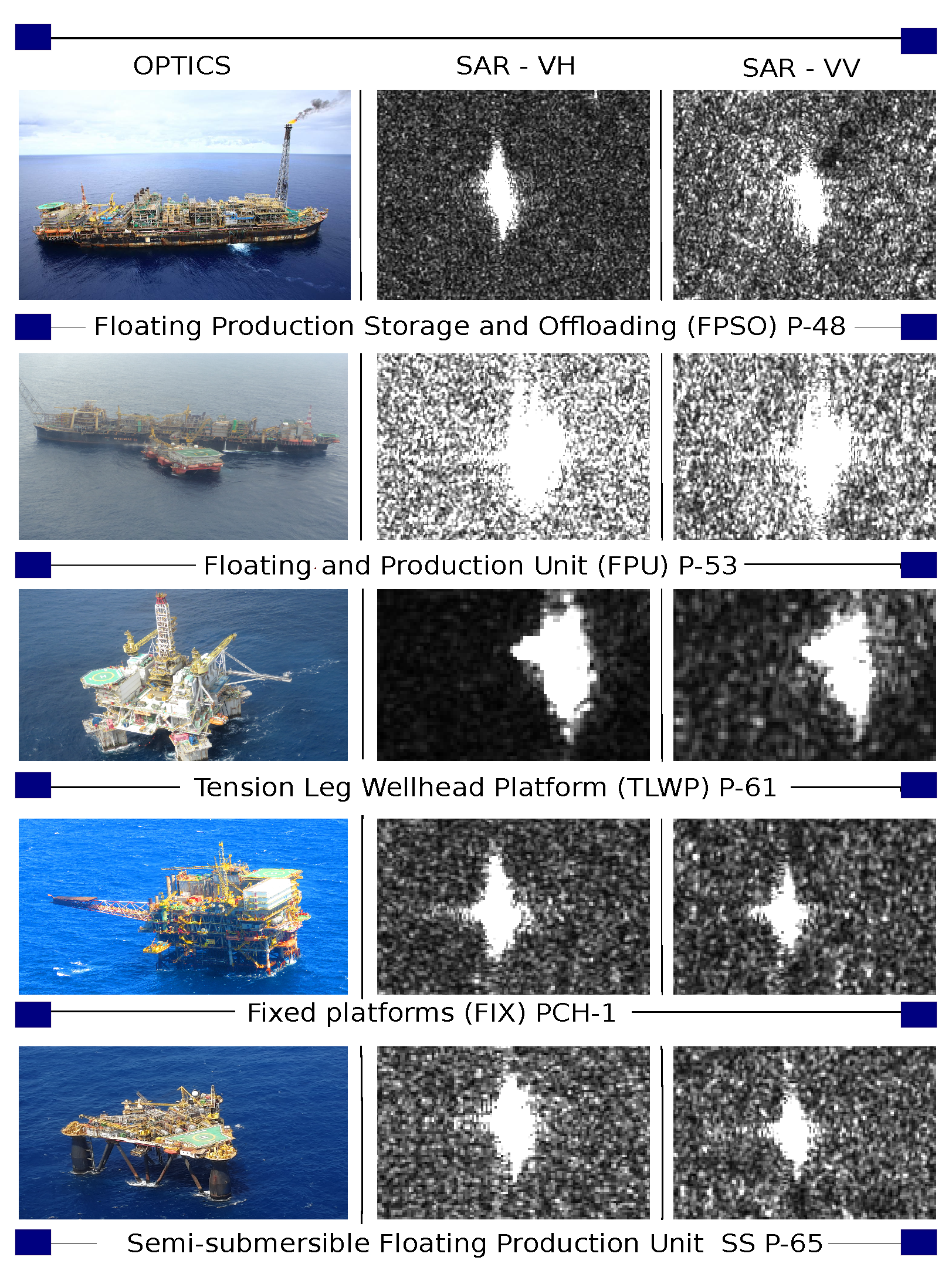
Following the methodology employed in [26], the original amplitude-type images were transformed into sigma-zero (dB) images. Figure 4 presents an optical image and its respective SAR image for the following targets: (i) Floating Production Storage and Offloading (FPSO) platforms P-48; (ii) Floating and Production Unit (FPU) P-53; (iii) Tension Leg Wellhead Platform (TLWP) P-61; (iv) Fixed Platform (FIX) PCH-1; and (v) Semisubmersible (SS) P-65. These images were collected with the ground-range-detected product; interferometric wide swath mode; high spatial resolution ($20\mathrm{m}\times 22\mathrm{m}$—range × azimuth); pixel spacing equal to $10\mathrm{m}\times 10\mathrm{m}$ in range and azimuth, respectively; and $5\times 1$ number of looks (the equivalent number of looks is 4.4 [30]).

The legends (${\upsilon }_1,{\upsilon }_2,{\upsilon }_3,{\upsilon }_4,{\upsilon }_5,{\upsilon }_6,{\upsilon }_7,{\upsilon }_8$) represent the images with VH polarization and the legends (${\iota }_1,{\iota }_2,{\iota }_3,{\iota }_4,{\iota }_5,{\iota }_6,{\iota }_7,{\iota }_8$) represent the images with VV polarization, taken on the dates mentioned in

Table 3. Number of targets extracted in each SAR image.

	Polarization
	VH			VV
SAR Image Date	Legend	Oil Rig	Ship	Legend	Oil Rig	Ship
20180430 at 08:04 a.m.	${\upsilon }_1$	42	50	${\iota }_1$	42	50
20180605 at 08:05 a.m.	${\upsilon }_2$	40	49	${\iota }_2$	40	49
20180512 at 08:05 a.m.	${\upsilon }_3$	40	48	${\iota }_3$	40	48
20171118 at 08:13 a.m.	${\upsilon }_4$	12	29	${\iota }_4$	12	29
20180524 at 08:05 a.m.	${\upsilon }_5$	38	11	${\iota }_5$	38	11
20180617 at 08:04 a.m.	${\upsilon }_6$	8	0	${\iota }_6$	8	0
20180622 at 08:13 a.m.	${\upsilon }_7$	13	0	${\iota }_7$	13	0
20180430 at 08:05 a.m.	${\upsilon }_8$	7	13	${\iota }_8$	7	13

.

2.2. Classification Tools

This section presents the classifier methods employed in this article. In particular, a classifier can be defined as a function f that maps the input vectors of features, $x\in \chi$, into the output class labels, $y\in \left\{1,2,\dots ,C\right\}$, where $\chi$ is the attribute space and C is the number of classes. Usually, it is assumed that $\chi ={\mathbb{R}}^D$ or $\chi ={\left\{0,1\right\}}^D$, that is, that the attribute vector is a vector of D real numbers or binary bits [32]. Classification is one of the most important topics in data mining, especially for large amounts of data (big data) applications. The main task of classification is to predict the labels of the test data based on the training data [33]. In the following, the employed classifiers in this study are presented. The first considered method is the SVM scheme, which is a class of statistical models first developed in the 1960s by Vladimir Vapnik [34] that can be used for classification [35]. SVM has become popular due to its applicability in a variety of contexts, such as extreme learning machines [34], automatic target recognition for CNN-based in SAR images [36], SAR ATR, and independent component analysis [37].

The second scheme applied in our study is the DT, which is a nonparametric supervised learning method used for classification and regression [38].

The main idea of this algorithm is that the trees learn how to approximate a sine curve with a set of decision rules. They are visualized using a graph, which makes them easy to interpret. In addition, they require little previous information and can handle both numerical and categorical data. On the other hand, instability due to small variations in the data can cause changes in the tree [39,40].

Another employed method is the RF, which is a hybrid of the bagging algorithm and random subspace method and uses DT as a basis in the classification process [41]. In other words, RF is a combination of tree predictors, where each tree depends on the values of a random vector sampled independently with the same distribution for all the trees in the forest [42], that is, each tree is built from a sample, which is taken with replacement from the training set. Individual DTs have high variance and tend to overfit. However, the randomness injected into forests produces DTs with reduced prediction errors. Furthermore, increasing the number of trees can produce better accuracy results and limit the generalization error [42].

The NB and kNN methods were investigated in this study. The NB is one of the most efficient algorithms used in ML, classification, pattern recognition, and data mining, and it is based on Bayes’ theorem [43,44,45]. The kNN is a nonparametric classification method that has been used in different real-world applications due to its simplicity and efficiency [33,46]. The main idea of the kNN method is to predict the label of a test data point by the majority rule. In other words, the test data label is predicted with the main class with its k most similar training data points in the attribute space [33]. To avoid inaccurate prediction results, it is necessary to choose an appropriate value of k. A simple way to choose k is to load the algorithm several times with different values of k and select the one with the best result [47].

We also considered the LR scheme, which is a linear model useful for classification tasks. The sigmoid function is the basis for LR. Particularly, the logistic sigmoid function is expressed as

$$\sigma \left(x\right)=\frac{1}{1+exp\{-x\}},$$

(1)

where the input $x\in (-\infty ,\infty )$ produces results in the range of $\left[0,1\right]$. LR adds an exponential function at the linear regression, bounding the output $y_i\in \left[0,1\right]$, and $i=1,2,\dots ,n$, where n is the total number of training samples [48]. The relationship between the input and the predicted output for LR is presented as

$$\begin{array}{c}\hfill {\widehat{y}}_i=\sigma \left(\sum _{j=1}^n{x}_{ij}{w}_j+w_0\right),\end{array}$$

(2)

where $x_{ij}$ is the input given by an n-dimensional vector belonging to reals; $y_i$ is the current output value that is given by a one-dimensional array; ${\widehat{y}}_i$ is the predicted output value that is given by an array; $w_j$ is the weight parameters; and $w_0$ a bias term. Since the output is limited to the interval $\left[0,1\right]$, it can be interpreted as a probabilistic measure, that is, the LR is a variation of the linear regression [48].

This article also considered the AdaBoost (ADBST) classifier. ADBST is an adaptive boosting algorithm proposed by Freund and Schapire in 1999 [49], developed for binary classifications. The purpose of the classifier is to train predictors sequentially, trying to correct previous predictors and focusing on the most difficult cases. The algorithm increases the weight for training samples that have been misclassified, that is, the classifier learns from previous prediction errors [46]. The weight is associated with the degree of difficulty in getting it right. It builds a stronger classifier from a combination of weaker classifiers. If there are correct answers, then the classifier is rewarded. The process is repeated in T rounds, for $t=\left\{0,1,\dots ,T\right\}$, and n training samples. In each iteration of the algorithm, the weights are adjusted, and the samples are trained [50]. The final model is defined by the weighted majority of weak T learners, where their weights are adjusted during the training [46,50]. Initially, all training samples must have the same weight, so $w_i=1/n$, $\forall x_i$, $i=1,2,\dots ,n$. Then, the algorithm considers all possible classifiers and identifies the $f_i\left(x\right)$ that minimizes ${ϵ}_t$, which is the sum of the weights of the misclassified points. The weight ${\alpha }_t$ of the new classifier is expressed as

$$\begin{array}{c}\hfill {\alpha }_t=\frac{1}{2}ln\left(\frac{1-{ϵ}_t}{{ϵ}_t}\right),\end{array}$$

(3)

which depends on the accuracy with respect to the current set of measured points. The weights are then normalized as ${\sum }_{i=1}^n=w_i=1$, and as a result, we have a classifier with an error ${ϵ}_t\le {0.5}^3$. In the next round, incorrect classifications have their weights adjusted to make them more significant. Let ${\widehat{y}}_t$($x_i$) be a class—assuming values of 1 or $-1$—predicted for $x_i$, and $y_i$ be the correct value of the class. For the situation where ${\widehat{y}}_t$ (predicted) value is equal to $y_i$ (observed) value, the ${\widehat{y}}_t\left(x_i\right).y$ signal is a positive value; otherwise, it will assume a negative. The adjusted weights are expressed as $w_{i,t+1}^{\prime }=w_{i,t}exp\{-y_i{\alpha }_t{\widehat{y}}_t\left(x_i\right)\}$, before renormalizing them all, so that they continue to sum to 1, that is, $C={\sum }_{i=1}^n{w}_{i,t+1}^{\prime }$, and $w_{i,t+1}=w_{i,t+1}^{\prime }/C$ [50].

We also employed a neural network as a classification tool. A NET is a very complex technology that requires a large amount of data for the training process, which is based on how human neurons work, receiving a set of inputs that are used to predict one or more outputs [51]. One of the main uses of NETs is in grouping data into two or more classes. Neural networks can be trained in two ways: (i) supervised learning, where each training input vector is paired with a target vector or desired output, and (ii) unsupervised learning, where the net self-organizes to extract patterns from data with no target information. In the n-dimensional space, the input vectors are represented as $\left(x_1,x_2,\dots ,x_n\right)$ or x, and the coefficients or weights are represented as $\left(v_1,v_2,\dots ,v_n\right)$ or v, i.e., $\mathbf{x}.\mathbf{v}=y$ [52].

Finally, the stacking or stacked generalization technique is an ensemble method that combines multiple models to achieve better classification results [53,54], and this was also used in our study. This type of scheme can be more accurate than an individual classifier [55]. For instance, [56] demonstrates the efficiency of the technique by combining three different algorithms, DT, NB, and IB1 (a variation of the lazy algorithm).

2.3. Classification Setup

This section describes the methodology employed in this article, introducing the training and test groups and the steps used in the classification tools. To obtain the training and test groups, we adopted the methodology proposed in [26], where 50 groups were created randomly, resulting in 320 training images (80% of the total samples) and 80 test images (20% of the total samples). 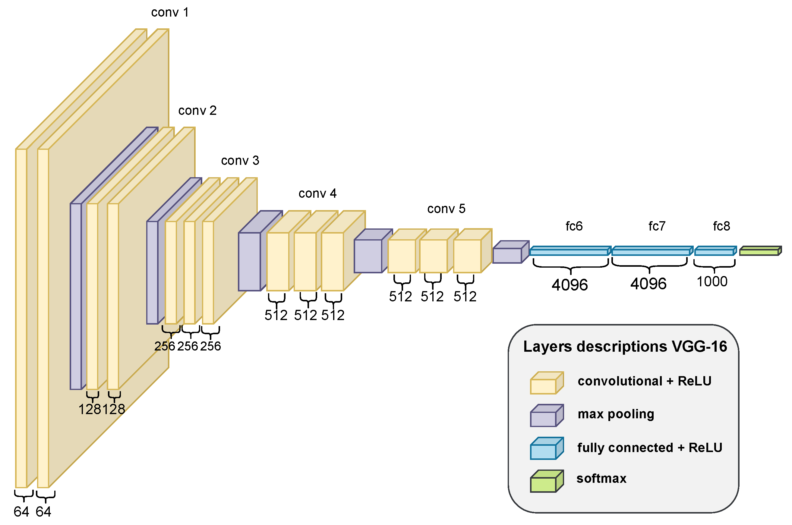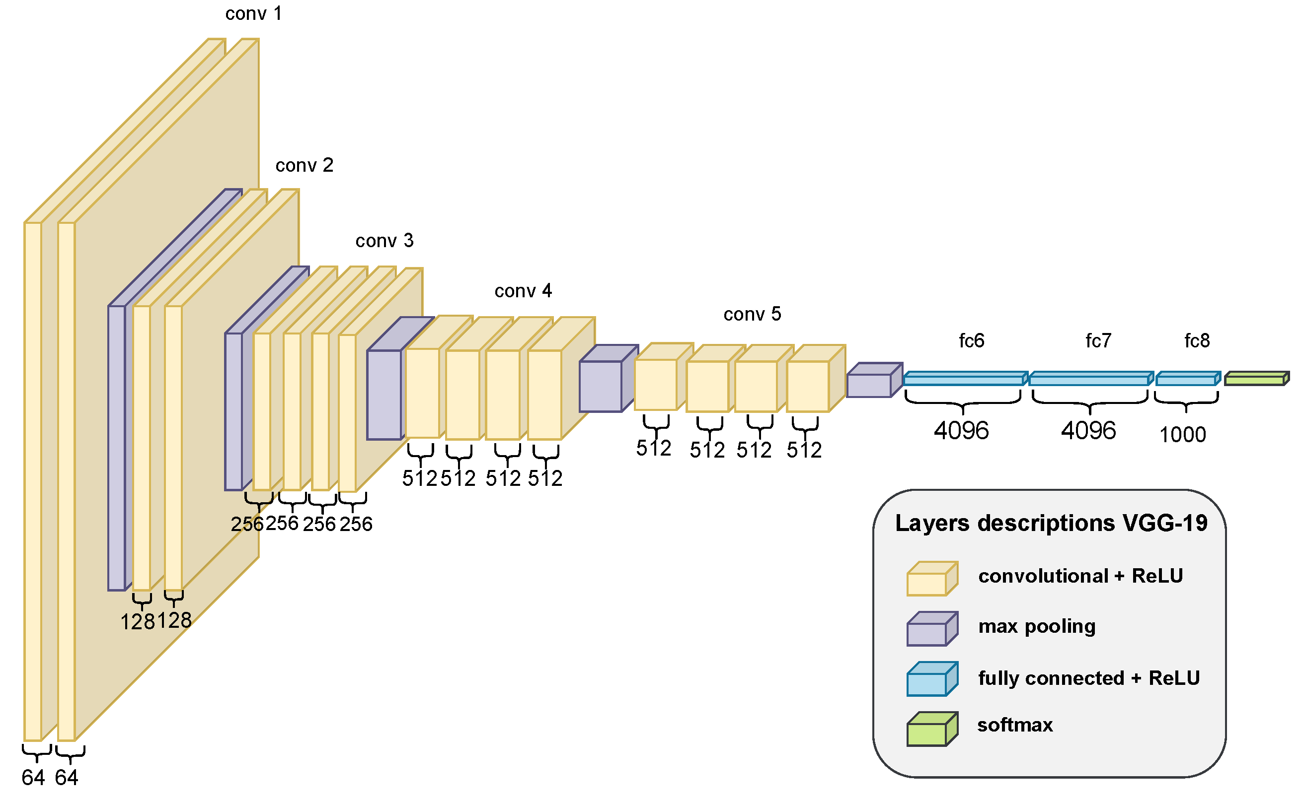Before starting the classification steps, the image attributes are extracted using CNN VGG-16 and VGG-19 [57]. A VGG is a CNN with a convolutional layer stacking with different levels of depth.

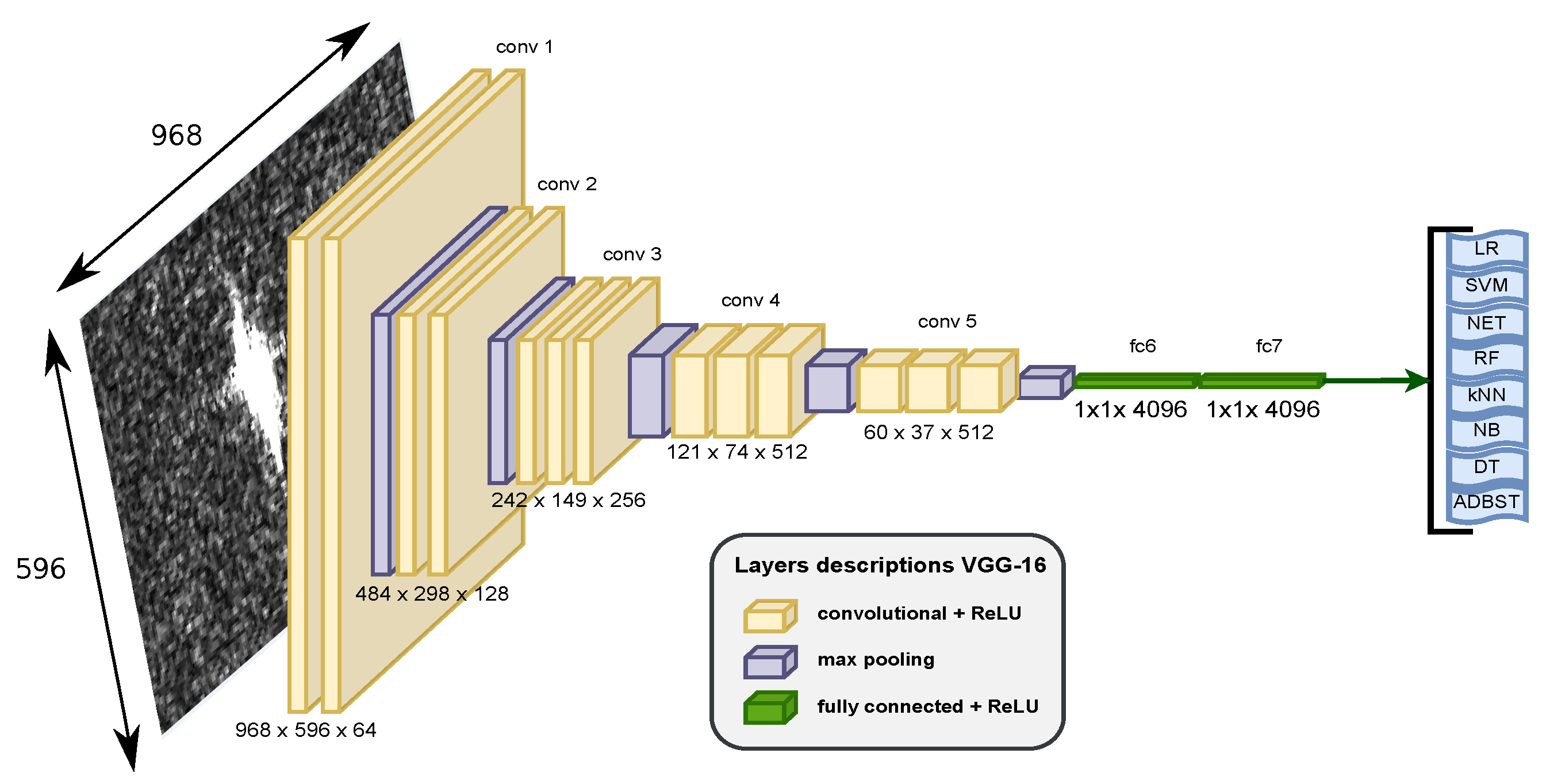
The difference between VGG-16 and VGG-19 is in the number of convolutional layers. More precisely, VGG-16 comprises 13 convolutional layers [58,59], while VGG-19 is made up of 16 convolutional layers [60,61]. This difference can be seen in Figure 5 and Figure 6. The VGG-16 is composed of: (i) conv 1—two convolutional layers with 64 channels; (ii) conv 2—two convolutional layers with 128 channels; (iii) conv 3—three convolutional layers with 256 channels; (iv) conv 4—three convolutional layers with 512 channels; (v) conv 5—three convolutional layers with 512 channels; (vi) fc6—4096 channels; (vii) fc7—4096 channels; and (viii) fc8—1000 channels. On the other hand, VGG-19 is composed of: (i) conv 1—two convolutional layers of 64 channels; (ii) conv 2—two convolutional layers with 128 channels; (iii) conv 3—four convolutional layers with 256 channels; (iv) conv 4—four convolutional layers with 512 channels; (v) conv 5—four convolutional layers with 512 channels; (vi) fc6—4096 channels; (vii) fc7—4096 channels; and (viii) fc8—1000 channels. In short, the difference between the two occurs in conv 3–5. The VGG architecture used in the research ends in the FC7 layer. Therefore, the FC7 layer with the embedding is the input for the classification algorithms, as shown in Figure 7.

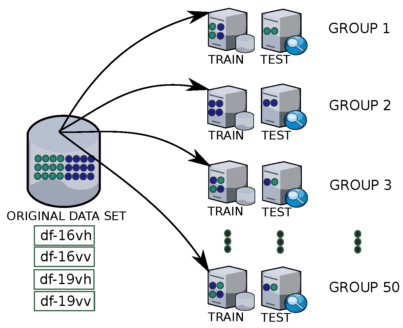
After extracting attributes with the CNNs, four different data sets are created, df-16vh, df–16vv, df-19vh, and df-19vv, which are the results of the combinations of the two CNNs, VGG-16/VGG-19, and the VH/VV polarizations.

The bootstrap technique was used to ensure reproducibility and to make sure that the classifiers are evaluated under the same conditions. Bootstrap is a random resampling technique with replacement from the primary dataset [39,62]. This technique makes it possible to estimate the empirical distribution of statistics [39,63]. In this work, each data set (i.e., df-16vh, df-16vv, df-19vh, df-19vv) is resampled 50 times, as described in Figure 8. Similar to [26], each resampling consists of 320 training samples and 80 test samples.

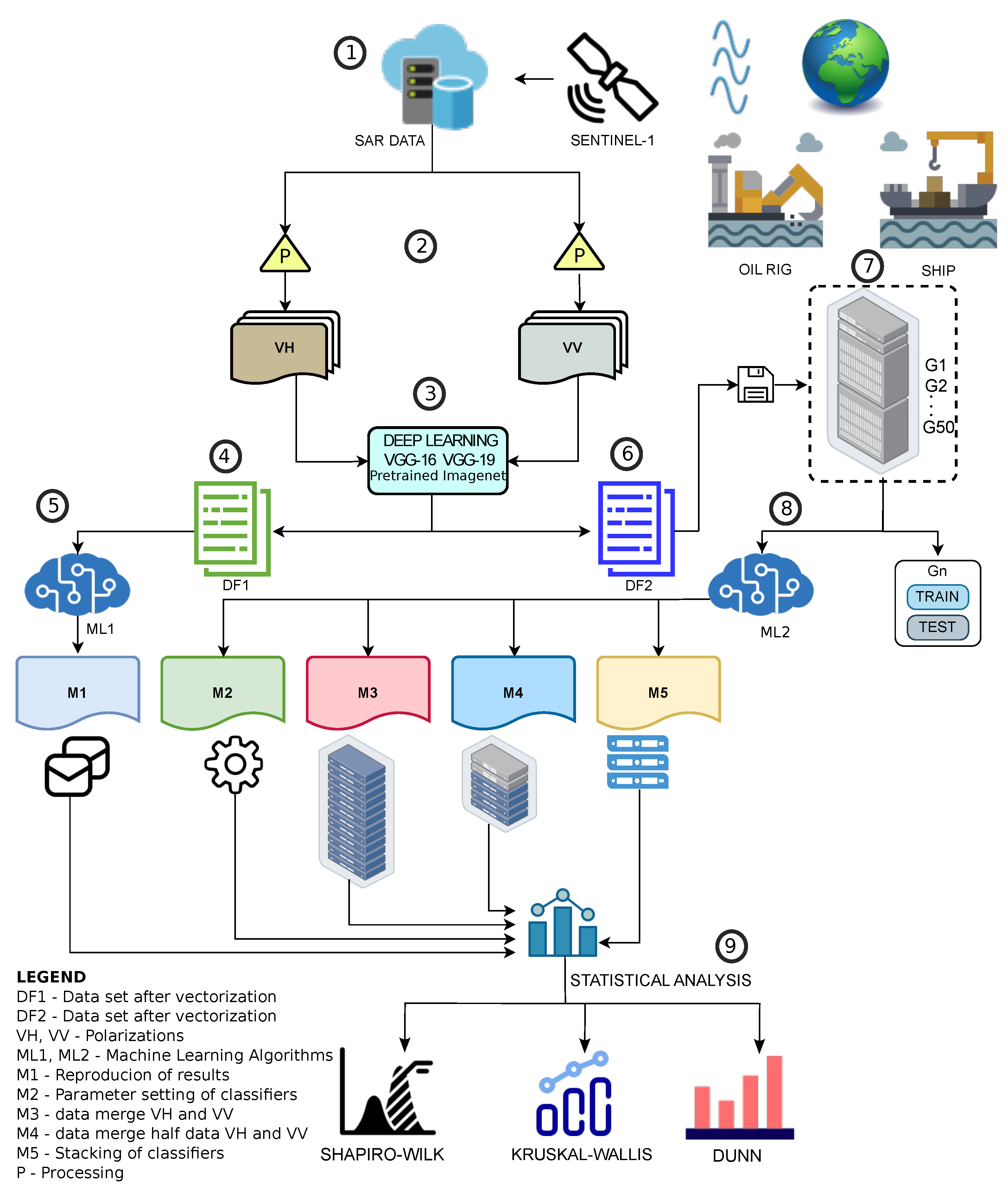
The methodology of this work is described in the items below and shown in Figure 9.

(1)

Data set

The data set consists of eight Sentinel-1 SAR images in VH polarization and eight in VV polarization, GRD product, IW mode, obtained through ESA’s Copernicus project [64] in the periods listed in Table 3.

(2)

Preprocessing

The original data set went through a calibration process using SNAP software (Sentinel Application Platform) to transform the amplitude image into zero-sigma. Then, the cutouts of the targets were made manually through SNAP. The dimensions of the images are displayed in

Table 4. Size of image patches.

Dimension: Range × Azimuth
912 × 596 pixels
968 × 596 pixels
939 × 596 pixels
901 × 596 pixels
930 × 596 pixels
944 × 596 pixels
985 × 596 pixels
1057 × 596 pixels

. The identification of oil platforms is through geolocation (latitude × longitude) provided by the ANP [65]. Targets without geolocation are considered ships. The number of targets extracted in each SAR image is presented in Table 3. Each patch is individually exported as a TIFF image. The types of platforms in the images are listed in

Table 5. Distribution of platform patches between training and testing samples.

		Polarization								Total
		VGG-16VH		VGG-16VV		VGG-19VH		VGG-19VV
Id	Oil Rig	Test	Train	Test	Train	Test	Train	Test	Train
1	FIX PCA1		2		2		2	1	1	8
2	FIX PCA2	1	1		2		2		2	8
3	FIX PCH1	2	3	2	3	2	3	1	4	20
4	FIX PCP1	1	2	1	2		3		3	12
5	FIX PCP2		3		3		3	1	2	12
6	FIX PEREGRINOA		1		1		1		1	4
7	FIX PNA1	1	4	2	3		5	2	3	20
8	FIX PNA2	1	4		5		5	1	4	20
9	FIX POLVOA		1		1		1		1	4
10	FIX PPG1	1	4		5	1	4		5	20
11	FIX PPM1		2	1	1		2		2	8
12	FIX PRA1	1	3		4	2	2	1	3	16
13	FIX PVM1	1	4	1	4		5		5	20
14	FIX PVM2	2	3	1	4		5	1	4	20
15	FIX PVM3	1	4		5	1	4		5	20
16	FPSO CAPX	1	1	2		1	1	1	1	8
17	FPSO CDAN	1	2		3	2	1	1	2	12
18	FPSO DYNAMIC		1		1		1	1		4
19	FPSO ESPST		2		2		2		2	8
20	FPSO FPF	3	2	1	4		5		5	20
21	FPSO FPNIT		3	1	2		3	1	2	12
22	FPSO FPRJ		4	2	2		4	1	3	16
23	FPSO FPRO	2	2	1	3	1	3	2	2	16
24	FPSO FRADE	1	1		2		2	1	1	8
25	FPSO OSX3		1		1		1		1	4
26	FPSO P31		4		4		4		4	16
27	FPSO P33	1	3	1	3	1	3	3	1	16
28	FPSO P35		4	1	3	1	3	1	3	16
29	FPSO P37		4		4		4		4	16
30	FPSO P43	1	3		4		4	2	2	16
31	FPSO P47		3	1	2		3	2	1	12
32	FPSO P48	1	2	1	2		3	1	2	12
33	FPSO P49		1	1			1		1	4
34	FPSO P50		4	1	3	1	3	1	3	16
35	FPSO P54		3		3	1	2		3	12
36	FPSO P57		3		3	1	2		3	12
37	FPSO P58		3		3	1	2	1	2	12
38	FPSO P62		5	3	2	1	4	2	3	20
39	FPSO P63		1		1		1	1		4
40	FPSO P64		1	1			1		1	4
41	FPSO PEREGRINO		1	1		1			1	4
42	FPSO POLVO		1	1			1		1	4
43	FPU P53	1	2		3	2	1		3	12
44	FSO MACAE		4		4		4	1	3	16
45	FSO P32	1	1		2		2		2	8
46	FSO P38		3	1	2		3	1	2	12
47	SS P07	2	3		5	2	3		5	20
48	SS P08	1	4	1	4	3	2	1	4	20
49	SS P15		5	2	3	1	4		5	20
50	SS P18	2	2		4	2	2	2	2	16
51	SS P19	1	3	1	3		4		4	16
52	SS P20	3	2	1	4		5	2	3	20
53	SS P25	1	3	2	2	2	2		4	16
54	SS P26	1	3	1	3	1	3	1	3	16
55	SS P40	1	3	1	3	2	2	1	3	16
56	SS P51	1	3	1	3	1	3		4	16
57	SS P52		2		2	2			2	8
58	SS P55		4		4		4		4	16
59	SS P56	1	3	1	3	1	3		4	16
60	SS P65	1	3	1	3	3	1	1	3	16
61	TWLP P61		1		1		1		1	4
	Total	40	160	40	160	40	160	40	160	800

. TIFF image patches form the VH and VV data sets from platforms and ships.

(3)

Extraction of attributes

The VH and VV image patches are the input of two CNNs, VGG-16 and VGG-19, pre-trained in the ImageNet data set, which extract features and generate four data sets: df-16vh, df-16vv, df-19vh, and df-19vv. Figure 5 presents an example of the application of VGG-16. It is noticed that the VGG-16 of our research uses the FC7 layer to provide the attributes to the classification algorithms. In this article, VGG-19 also uses the FC7 layer to provide the attributes to the classification algorithms.

(4)

Formation of train and test samples

The proportion of 80% (training) and 20% (test) is considered. Training and testing samples are generated randomly. This was the methodology applied by [26].

(5)

Classification with the M1 method

In this method, ML techniques are applied in order to reproduce the results of [26].

(6)

Bootstrap formation

The samples vectored in the four data sets (df-16vh, df-16vv, df-19vh, df-19vv) are randomly distributed with replacement in 50 bootstrap groups and saved to submit the classifiers to the same reproducibility conditions. Table 5 presents the distribution of platforms between training and test samples in a bootstrap group.

(7)

Bootstrap and formation of train and test samples

Each of the 50 bootstrap groups comprises subsets of the original data sets (df-16vh, df-16vv, df-19vh, df-19vv).

(8)

Classification with the M2-M5 method

ML techniques are applied to the M2–M5 methods considering the kNN, SVM, LR, DT, RF, NB, NET, and ADBST algorithms.

(9)

Statistical analysis

Statistical analysis is performed using the Shapiro–Wilk methods (normality analysis); Kruskal–Wallis (significant difference analysis); and Dunn (identifies who owns differs). For brevity purposes, the two best results in each method (M1–M5) were considered.

To perform the classification, we used the following five methods, namely M1, M2, M3, M4, and M5, defined as follows:

(M1)

Aiming at reproducing the results obtained by [26], the LR, SVM, RF, kNN, DT, and NB classifiers were used with parameters in the default setting. To the best of our knowledge, [26] is the only study available in the literature for maritime target classification in Sentinel-1 SAR data based on ML techniques. For comparison purposes, in this method, the samples were randomly generated only at the time of classification and were not saved, and the parameters of the applied classification tool are the ones predefined as default in the Orange Canvas software [66], which are described in

Table 6. Default parameters available of the employed classification methods in Orange Canvas software [66].

Classifier	Parameter	Value
kNN	Number of neighbors	3
	Distance	Euclidean
	Weight	Uniform
DT	Tree type	Binary
	Minimum instances per sheet	2
	Minimum instances for splitting a node	5
	Tree depth limit	100 node levels
	Stop criteria based on majority	95%
RF	Number of trees	10
	Minimum instances for splitting a node	5
SVM	Cost	1
	Regression loss epsilon	0.1
	Kernel	RBF
	Numerical tolerance	0.001
	Number of interactions	100
NB	No parameters	-
LR	Regularization method	Ridge (L2)
	Force	1

.

(M2)

The number of algorithms used in M1 was increased with the addition of the NET and ADBST methods. In this step, an extensive computational search was performed, varying the parameters of the considered classification algorithms, aiming to maximize their performance. The employed parameters are presented in

Table 7. Parameters employed in the classification tools.

Classifier	Parameter	Value
RF	Number of trees	10, 50, 100, 200, 300, 400
		500, 600, 700, 800, 900
		1000, 1100, 1200, 1300
kNN	Number of neighbors	3, 5, 7, 10
	Distance used	Euclidean and Manhattan
ADBST	Number of estimators	10, 50, 100
LR	Strength	0.6, 1, 10, 50, 100, 200
NET	Number of neurons	10, 50, 100, 200
SVM	Cost	1, 2, 3, 4, 5
	Kernel	RBF and SIGM
	Number of interactions	100 and 200
DT	Minimum instances per sheet	2, 5, 7, 10, and 20
NB	No parameters

. The basis for parameter adjustment is empirical and was optimized to improve the results presented by [26]. For example, [67] shows that 500 trees are a good choice for constituting the RF. However, this number can be increased to approximately 3000 to evaluate the results. For SVM and ADBST, [67] shows that the proper adjustment is made by gradually changing the parameter values. Indeed, there is no analytical methodology to reach optimal parameter values because the optimization depends on the data. This was evident when [68] optimized the parameters of SVM, kNN, and DT, demonstrating that the ideal values of the parameters can vary with the size of the training data.

(M3)

In this method, the training data set was expanded with the concatenation of all samples from the VH and VV data sets. The test data set remained unchanged.

(M4)

The training data set was extended with the concatenation of half of the samples of the VH and VV image data set. The test set remained with the same samples.

(M5)

The stacked generalization technique consists of combining several classifiers, aiming to obtain better classification results [53,56,69]. Since supervised classification is performed in all steps, the distribution of the training and test sets is done according to

Table 8. Distribution of the training and test samples.

		Samples
CNN	Pol	Total	Training			Test
			M1, M2,andM5	M3	M4
VGG-16	VH	400	320	640	160 (VH) + 160 (VV)	80
	VV	400	320			80
VGG-19	VH	400	320	640	160 (VH) + 160 (VV)	80
	VV	400	320			80

.

In this section, the numerical results are presented and discussed. To perform the maritime target classification in the Sentinel SAR data based on ML techniques, we extracted 4096 features from the images using CNNs VGG-16 and VGG-19, available in the Orange Canvas software [66]. For this architecture, the number of filters doubles after each max pool layer [20]. Consequently, from the data set generated by feature extraction, 50 distinct groups were defined, separated by networks VGG-16 and VGG-19, and polarizations VH and VV. Additionally, to perform the classification, we employed the tools described in Section 2.2 and the steps presented in Section 2.3.

To evaluate the performance of the employed methods, we considered the following metrics: area under the curve (AUC), accuracy (Acc), F1 score, precision, and recall. The mean for each metric was computed considering the 50 groups of data (randomly created, as mentioned in Section 2.3). Since all the results lead to the same conclusion, we decided only to discuss the Acc results in this section. The remaining results are detailed in Appendix A.

Finally, statistical analyses, such as the Shapiro–Wilk and Kruskal–Wallis tests, are presented to assess the overall performance of the methods. A flowchart with the stages of image acquisition, attribute extraction with DL algorithm, image classification methods, and statistical analysis of classification accuracy is presented in Figure 9.

Table 9. Optimized parameters in step M2.

		Parameter
		Classifier
CNN	Pol	kNN	LR	RF	SVM	DT	NET
VGG-16	VH	7-Manhattan	1	50	4-SIGM-200	7	10
	VV	3-Manhattan	1	200	3-SIGM-200	5	50
VGG-19	VH	5-Manhattan	1	1200	1-SIGM-100	2	50
	VV	5-Euclidean	0.6	100	2-SIGM-200	5	100

presents the setups that optimize the performance of the tested methods. The parameters are the number of CNN layers and the polarization channel. The NB and ADBST methods parameters are not presented since NB has no configuration parameters, and ADBST presented the same results, regardless of the parameter setup.

Considering the parameters displayed in Table 9,

Table 10. Overall summary of accuracy mean results of the employed classification methods for the VGG—16VH, 16VV, 19VH, and 19VV SAR images. The best results are highlighted in bold. The symbol (i) “-” indicates that the classification result is absent, and (ii) “x” indicates which classifiers are combined to obtain the final result with the stacked generalization technique in step M5.

	Classifier	Mref	M1	M2	M3	M4	M5
VGG - 16VH	kNN	0.772	$0.778\pm 0.04$	$0.792\pm 0.04$	$0.768\pm 0.03$	$0.772\pm 0.04$
	LR	0.864	$\mathbf{0.852}\pm 0.03$	$\mathbf{0.855}\pm 0.03$	$0.627\pm 0.08$	$\mathbf{0.846}\pm 0.04$	x
	NB	0.698	$0.711\pm 0.05$	$0.696\pm 0.04$	$0.691\pm 0.04$	$0.687\pm 0.05$
	RF	0.802	$0.792\pm 0.04$	$0.818\pm 0.04$	$\mathbf{0.799}\pm 0.04$	$0.780\pm 0.04$	x
	SVM	0.804	$\mathbf{0.806}\pm 0.04$	$\mathbf{0.838}\pm 0.03$	$0.785\pm 0.04$	$0.792\pm 0.04$	x
	DT	0.750	$0.744\pm 0.04$	$0.738\pm 0.04$	$0.757\pm 0.05$	$0.724\pm 0.05$	x
	ADBST	–	–	$0.732\pm 0.05$	$0.739\pm 0.05$	$0.726\pm 0.04$
	NET	–	–	$0.838\pm 0.03$	$\mathbf{0.840}\pm 0.03$	$\mathbf{0.830}\pm 0.03$
	Stack	–	–	–	–	–	$0.844\pm 0.03$
VGG - 16VV	kNN	0.694	$0.701\pm 0.04$	$0.708\pm 0.04$	$\mathbf{0.748}\pm 0.04$	$0.700\pm 0.05$
	LR	0.781	$\mathbf{0.782}\pm 0.04$	$\mathbf{0.783}\pm 0.03$	$0.608\pm 0.07$	$\mathbf{0.783}\pm 0.04$	x
	NB	0.660	$0.645\pm 0.04$	$0.657\pm 0.04$	$0.656\pm 0.04$	$0.658\pm 0.05$
	RF	0.704	$0.695\pm 0.05$	$0.740\pm 0.04$	$0.728\pm 0.05$	$0.703\pm 0.04$	x
	SVM	0.723	$\mathbf{0.714}\pm 0.04$	$0.760\pm 0.03$	$0.729\pm 0.04$	$0.722\pm 0.04$	x
	DT	0.659	$0.642\pm 0.04$	$0.654\pm 0.04$	$0.676\pm 0.05$	$0.668\pm 0.04$	x
	ADBST	–	–	$0.650\pm 0.05$	$0.688\pm 0.05$	$0.667\pm 0.05$
	NET	–	–	$\mathbf{0.784}\pm 0.03$	$\mathbf{0.776}\pm 0.04$	$\mathbf{0.757}\pm 0.04$
	Stack	–	–	–	–	–	$0.763\pm 0.03$
VGG - 19VH	kNN	0.801	$0.801\pm 0.04$	$0.802\pm 0.04$	$0.793\pm 0.04$	$0.788\pm 0.04$
	LR	0.841	$\mathbf{0.851}\pm 0.03$	$\mathbf{0.842}\pm 0.03$	$0.641\pm 0.09$	$\mathbf{0.845}\pm 0.03$	x
	NB	0.707	$0.699\pm 0.05$	$0.704\pm 0.04$	$0.707\pm 0.04$	$0.698\pm 0.04$
	RF	0.815	$0.806\pm 0.03$	$0.833\pm 0.05$	$\mathbf{0.810}\pm 0.04$	$0.804\pm 0.03$	x
	SVM	0.824	$\mathbf{0.816}\pm 0.04$	$\mathbf{0.849}\pm 0.03$	$0.789\pm 0.04$	$0.799\pm 0.04$	x
	DT	0.776	$0.762\pm 0.04$	$0.765\pm 0.04$	$0.775\pm 0.04$	$0.758\pm 0.04$	x
	ADBST	–	–	$0.768\pm 0.05$	$0.770\pm 0.05$	$0.752\pm 0.04$
	NET	–	–	$0.836\pm 0.04$	$\mathbf{0.844}\pm 0.04$	$\mathbf{0.833}\pm 0.03$
	Stack	–	–	–	–	–	$0.841\pm 0.03$
VGG - 19VV	kNN	0.713	$0.713\pm 0.04$	$0.724\pm 0.04$	$0.763\pm 0.04$	$0.710\pm 0.04$
	LR	0.774	$\mathbf{0.766}\pm 0.04$	$\mathbf{0.768}\pm 0.06$	$0.624\pm 0.07$	$\mathbf{0.773}\pm 0.05$	x
	NB	0.643	$0.653\pm 0.04$	$0.652\pm 0.04$	$0.658\pm 0.04$	$0.657\pm 0.04$
	RF	0.719	$0.717\pm 0.05$	$0.751\pm 0.05$	$0.742\pm 0.05$	$0.727\pm 0.05$	x
	SVM	0.737	$\mathbf{0.731}\pm 0.05$	$0.754\pm 0.06$	$\mathbf{0.766}\pm 0.04$	$0.746\pm 0.05$	x
	DT	0.670	$0.667\pm 0.05$	$0.663\pm 0.05$	$0.706\pm 0.04$	$0.692\pm 0.05$	x
	ADBST	–	–	$0.640\pm 0.05$	$0.698\pm 0.04$	$0.680\pm 0.04$
	NET	–	–	$\mathbf{0.761}\pm 0.06$	$\mathbf{0.777}\pm 0.04$	$\mathbf{0.761}\pm 0.05$
	Stack	–	–	–	–	–	$0.761\pm 0.04$

shows the Acc mean values of 50 classification results; the best results are highlighted in bold. The classifiers that excelled in classification results were LR, NET, SVM, RF, and kNN, presenting a classification gain of 32.5%, 32.5%, 17.5%, 15.5%, and 2.5%, respectively.

Comparing our results with [26], the accuracy of the CNN VGG-16 was increased by 7.7% and 4.2% for the M4-kNN (VV polarization) and M2-SVM (VH polarization), respectively. For the CNN VGG-19, the gains are about 7.0% and 3% for the M4-kNN (VV polarization) and M2-SVM (VH polarization), respectively. In methods M3 and M4, there is an upgrade in the variability of the samples and the accuracy of the classification results. The stacking technique presents accuracy results ranging from 76.1% to 84.1%. Compared with the results shown in [26], the stacking technique does not excel only for the LR scheme.

Therefore, the RF, SVM, and NET classifiers excel in all the evaluated scenarios, and the LR had poor performance in method M4. In summary, considering all the classification techniques, the following ones stand out: LR, SVM, NET, STACK, and RF, with the highest accuracy results ranging between 80.5% and 85.45% for all the tested scenarios.

The VH polarization presents better results in detecting targets, mainly on oil platforms formed by large metallic structures of complex geometry. In general, the brightness of the targets is more intense in the VH polarization, and the background (sea) in the VV polarization. Therefore, feature extraction is best represented in VH polarization in the VGG-16 and VGG-19 networks.

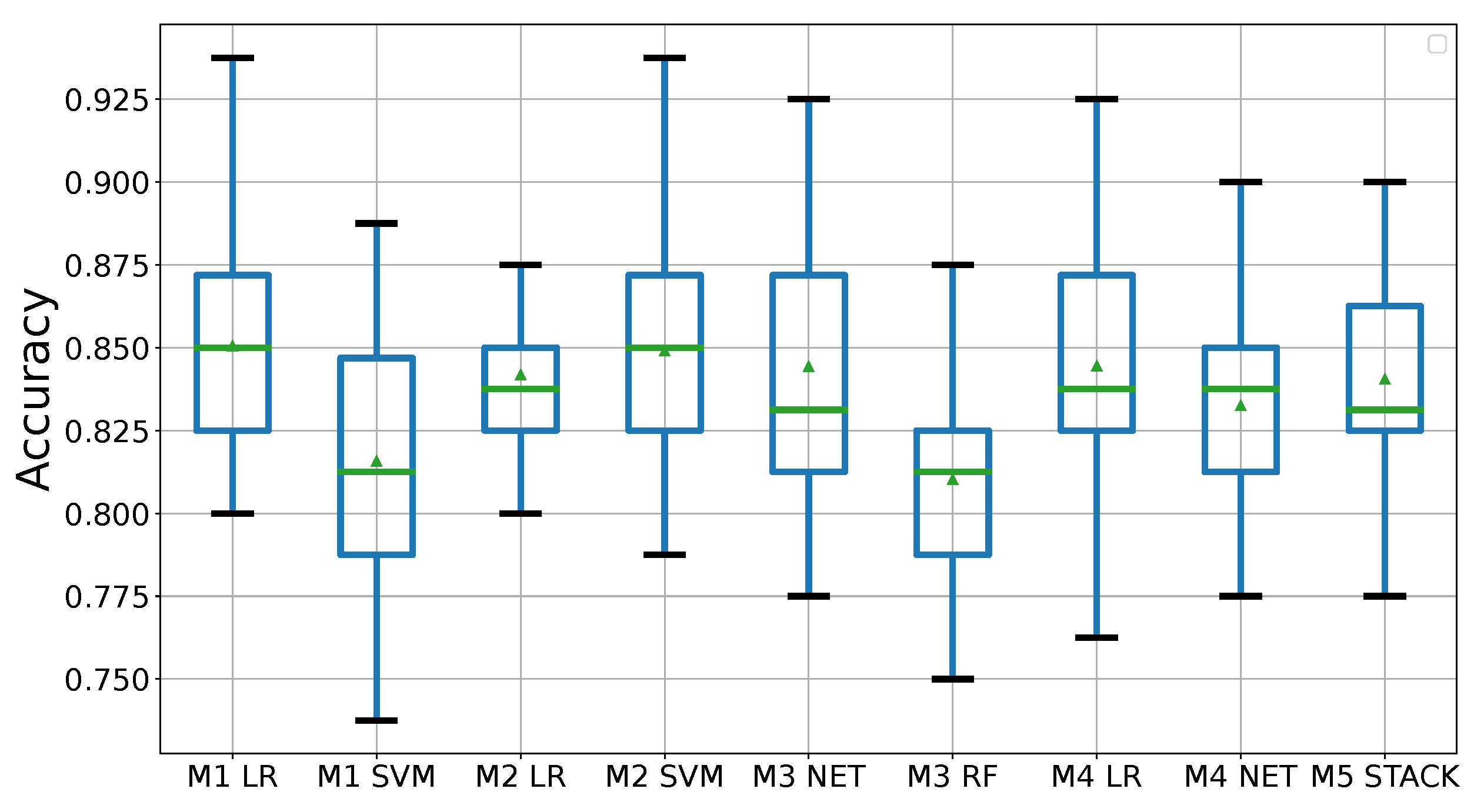
To emphasize the results highlighted in Table 10, Figure 10 demonstrates the top two classification results in each method with VGG-16VH. The other graphical results for VGG-19VH, VGG-16VV, and VGG-19VV are presented in Appendix A.

Complementing the results of Table 10,

Table 11. Overall summary of the average of all metrics employed in the classification method—method M1.

					Classifier
Method	CNN-Pol	Metric	kNN	LR	NB	RF	SVM	DT
M1	VGG-16VH	AUC	0.837	0.928	0.738	0.876	0.897	0.719
		F1	0.776	0.851	0.707	0.791	0.803	0.743
		Precision	0.782	0.855	0.721	0.795	0.826	0.747
		Recall	0.778	0.852	0.711	0.792	0.806	0.744
	VGG-16VV	AUC	0.746	0.873	0.663	0.767	0.802	0.633
		F1	0.700	0.781	0.638	0.694	0.712	0.641
		Precision	0.703	0.785	0.657	0.697	0.722	0.645
		Recall	0.701	0.782	0.645	0.695	0.714	0.642
	VGG-19VH	AUC	0.842	0.923	0.737	0.886	0.911	0.723
		F1	0.800	0.850	0.695	0.805	0.814	0.761
		Precision	0.803	0.852	0.708	0.809	0.825	0.766
		Recall	0.801	0.851	0.699	0.806	0.816	0.762
	VGG-19VV	AUC	0.761	0.850	0.679	0.793	0.809	0.652
		F1	0.711	0.765	0.647	0.716	0.730	0.666
		Precision	0.718	0.769	0.666	0.720	0.734	0.670
		Recall	0.713	0.766	0.653	0.717	0.731	0.667

displays the average of the classification results for the M1 method with the CNN VGG-16/VGG-19 and the classification metrics (AUC, F1 Score, Precision, and Recall). In addition, it reproduces the results of [26], using the same training/testing and classification data generation approach. Each metric is calculated for the six classifiers (kNN, LR, NB, RF, SVM, and DT). As in [26], LR is the classifier with the best performance. Furthermore, it is observed that the results with VH polarization are superior to those with VV polarization. Methods M2 to M5 present result tables with the same structure as M1 for the metrics (AUC, F1 Score, Precision, and Recall). Therefore, tables are included in Appendix A.

3. Results and Discussion

To further evaluate the performance of the tested methods, we considered the Kruskal–Wallis and post hoc Dunn’s tests to identify if the employed methods present significantly different mean behavior in terms of accuracy in comparison with the approaches described in [26]. Both tests are widely explored in several non-Gaussian signal processing applications for comparison purposes of machine learning tools, such as in [70,71,72,73,74]. To verify the normality of the data, we performed the Shapiro–Wilk test, which indicates that 70%, 10%, 30%, and 30% of the VGG-16VH, VGG-16VV, VGG-19VH, and VGG-19VV data cannot be modeled by the normal distribution, respectively. For all the employed tests, we set the significance level equal to 0.05, which is a convenient cutoff level to reject the null hypothesis [75].

Table 12. Kruskal–Wallis and Dunn’s test results, comparing the proposed methods with the approaches presented in [26]. For brevity, only the cases with a significant difference in the mean behavior are displayed.

M	Classifier	M	Classifier	p-Value	M	Classifier	M	Classifier	p-Value
VGG-16VH					VGG-19VH
p-value <0.001					p-value < 0.001
1	SVM	2	LR	<0.001	1	SVM	2	SVM	0.003
1	SVM	2	SVM	0.027	1	LR	3	RF	<0.001
1	SVM	3	NET	0.008	1	NET	3	RF	0.006
1	LR	3	RF	<0.001	1	SVM	4	LR	0.024
1	SVM	4	LR	<0.001
1	LR	4	NET	0.041
VGG-16VV					VGG-19VV
p-value < 0.001					p-value < 0.001
1	SVM	2	LR	<0.001	1	SVM	2	LR	0.009
1	SVM	2	NET	<0.001	1	SVM	3	NET	<0.001
1	LR	3	kNN	0.021	1	SVM	3	SVM	0.047
1	SVM	3	kNN	0.026	1	SVM	4	LR	0.008
1	SVM	3	NET	<0.001
1	SVM	4	NET	<0.001

shows the p-values of the Kruskal–Wallis and Dunn’s tests for the results reproduced from [26] (M1) and the proposed tools; for brevity, just the significant results are displayed. Among them, SVM results in an accuracy gain of 4.17%, 3.94%, and 3.03% for VGG-16VH (M2), VGG-19VV (M4), and VGG -19VH (M2), respectively, in comparison with the results presented in [26].

Another analysis to consider is comparing the methods that present the best performances. For VGG-16VH (M2), the LR classifier presents gains of 0.35%, 1.76%, 0.97%, and 1.24% about M1, M3, M4,and M5, respectively. For VGG-19VH (M1), the LR classifier presents gains of 0.18%, 0.77%, 0.65%, 1.13% over M2, M3, M4, and M5, respectively.

The performed analysis and statistical tests highlight that the applied schemes presented competitive performance when compared with [26], which, to the best of our knowledge, is the only study available in the literature related to detecting maritime targets in Sentinel-1 SAR images from the Campos Basin.

4. Conclusions

This article applied machine learning algorithms to classify maritime targets in Pol-SAR images (VH and VV) obtained with the Sentinel-1 system. The classifiers were evaluated considering five different methods (M1, M2, M3, M4, M5). As a pre-stage, the features were extracted using two CNN algorithms: VGG-16 and VGG-19. The classifiers were assessed in terms of accuracy. The RF, SVM, and NET classifiers excelled in all the evaluated scenarios over the reference methods, and the LR classifier performed poorly in M3. The classification results for all the tested classifiers except LR presented mean accuracy values above 80%, which were 1.44 times better than the baseline results in VGG-16VH and 1.55 better in VGG-19VH. VH polarization stands out in the classification of maritime targets, as oil platforms and ships have higher brightness (i.e., higher backscattering) because of their geometries formed by large metallic structures. With the parameters optimization, the tested classifiers showed more accurate classification results. The stacking technique also showed satisfactory accuracy results.