Distribution and Attribution of Earlier Start of the Growing Season over the Northern Hemisphere from 2001–2018

Abstract

The start of the growing season (SOS) is a vital ecological indicator for climate change and the terrestrial ecosystem. Previous studies have reported that the SOS over the Northern Hemisphere (NH) has experienced remarkable changes in the past few decades. However, because of the different spatial and temporal coverages of existing SOS studies, a coherent and robust account for SOS changes in the NH has been lacking. Using satellite-retrieved vegetation-phenology datasets, ground observations, and several auxiliary datasets, this study evaluated the performance of the latest MODIS vegetation-dynamics dataset (MCD12Q2-C6) and explored the distribution and attribution of the SOS to climate change over the NH for the period 2001–2018. The validation results using the Chinese Ecosystem Research Network (CERN) and Lilac-leafing observations (Lilac) displayed that the MCD12Q2-C6 has a good performance in SOS monitoring over the NH mid-latitudes. Meanwhile, evidence from MCD12Q2-C6 pointed out that the SOS was advanced by 2.08 days on average over the NH during 2001–2018, especially for Europe, China, and Alaska, United States. In addition, detailed-sensitivity analysis showed that the increased surface air temperature (T_s) (−1.21 ± 0.34 days °C⁻¹) and reduced snow-cover fraction (S_c) (0.62 ± 0.29 days%⁻¹) were the key driving factors of the observed SOS changes over the NH during 2001–2018. Compared with T_s and S_c, the role of total precipitation (P_t) was minor in dominating the spring vegetation-phenology changes at the same period. The findings of this study contribute to our understanding of the responses of SOS to the competing changes of T_s, P_t, and S_c over the NH.

1. Introduction

The start of the growing season (SOS), usually defined as the period of the year when plants grow successfully or the vegetation index first crosses 15% of the segment-vegetation-index amplitude by Moderate Resolution Imaging Spectroradiometer (MODIS) observation [1], is a vital indicator of terrestrial ecosystems that is related to productivity gradients [2], surface radiation and evapotranspiration [3], ecosystem atmospheric-carbon exchange and energy-budget estimation [4,5], surface warming [6,7], terrestrial-biosphere models simulation [8], and human activities in vegetation management [9,10], as well as several climate anomalies including fire disturbance [11], dry deposition [12], and heat waves [13]. Moreover, the SOS has become an important tool by which to measure both the impact of climate change on ecosystems and the feedback of ecosystems to the climate system [14,15]. Therefore, accurate information on the SOS is vital for both ecosystem monitoring and climate-change detection against the rapid climate-change background.

Published studies have reported that the SOS over the Northern Hemisphere (NH) has experienced remarkable changes in the past few decades. At continental scales, Schwartz et al. [16] concluded that the SOS advanced across most temperate NH land regions during 1955–2002. Jeong et al. [17] found that the SOS advanced by 5.2 days during the early period of 1982–1999 in the NH, but this magnitude reduced to only 0.2 days in the later period of 2000–2008. Meanwhile, Wang and Fensholt [18] reported that changes in the SOS were biome-specific in the NH (>30°N) during 1982–2013, indicating complex relationships and interactions that are induced by ongoing climate change and increasingly intensive human disturbances. At the regional scale, SOS anomalies in high latitudes, including the Arctic and boreal ecosystems [19,20,21] and Europe [22,23,24], and middle latitudes, including eastern China [25] and the Tibetan Plateau [26,27,28], have been explored separately. However, due to the different temporal and spatial coverages of the above-mentioned studies, existing SOS studies are difficult to compare. Consequently, a coherent and robust account for SOS changes in the NH has been lacking.

Satellite-retrieved vegetation-phenology datasets are an inevitable choice in SOS studies for their advantages in providing spatially explicit and temporally rich information on vegetation dynamics and patterns for landscapes at regional and global scales [29]. Currently, the MODIS vegetation-dynamics Collection 5 (MCD12Q2-C5) [30] and Collection 6 (MCD12Q2-C6) [1], as well as the National Aeronautics and Space Administration Making Earth System Data Records for Use in Research Environments (MEaSUREs) Vegetation Index and Phenology (VIP) [31], are the only available long-term satellite-derived vegetation phenology products. Although the Visible Infrared Imaging Radiometer Suite [32] and harmonized Landsat 8 and Sentinel-2 imagery [33] provide land-surface phenology with finer spatial resolution at 500 m and 10–30 m, their temporal coverage is too short to diagnose SOS changes at a continental scale. In addition to the well-developed vegetation-phenology datasets, the normalized-difference vegetation index (NDVI) from MODIS [27,34,35], the Global Inventory Monitoring and Modeling System 3rd Generation (GIMMS 3g) [28,36,37], and the French ‘Système Probatoire d’Observation de la Terre’—VEGETATION (SPOT-VGT) [2] are also employed in SOS dynamics studies, with the help of vegetation-phenology-retrieval algorithms. Nonetheless, subject to the high spatial heterogeneity of vegetation dynamics and a shortage of ground observations, their performance and consistency in SOS monitoring remains unclear.

Accompanied by SOS monitoring, the attribution of SOS anomalies has also drawn great attention in the past few years. Published studies have reported that global climate change is a primary driver of SOS variations in terrestrial ecosystems [37,38,39,40,41,42,43,44]. Several variables are attributed to SOS anomalies, e.g., land-surface temperature (T_s) [42,44,45,46], total precipitation (P_t) [46], water availability [40], spring snow-cover anomalies [43,44], and photoperiod [46,47,48] and temperature sensitivity [7,49] changes. Among the above-mentioned driving factors, T_s, P_t, and snow cover are basic and representative variables. For example, Krishnaswamy et al. [45] and Ren et al. [42] found that the SOS was strongly associated with T_s increase. Meanwhile, Chen and Yang [43] displayed that an advanced snow end date dominates SOS changes over the NH’s middle-to-high latitudes during 2001–2014. Although attribution analyses have been carried out at different scales, the mechanisms underlying hemispherical-scale SOS attribution remain debated. Whereas, due to the different spatial and temporal coverages of existing SOS studies, a coherent and robust account for SOS changes in the NH has been lacking.

The NH has experienced dramatic climate change over the past few decades, including intensifying Arctic amplification and extreme mid-latitudes weather [50,51], the shrinking of spring snow-cover extent [52,53], and the diminishing tight relationship between T_s and vegetation seasonality [49]. Changes in the climate system will significantly influence the distribution of the SOS. Therefore, it is crucially needed to clarify SOS anomalies and explore their driving factors over the NH in the context of a changing climate. To achieve this objective, we first estimated the performance of the latest MODIS vegetation-dynamics dataset using the Chinese Ecosystem Research Network (CERN) and Lilac-leafing observations (Lilac). Then, we explored the distribution and changes of the SOS over the NH for the period 2001–2018. Finally, we attributed SOS changes from three representative driving factors, T_s, P_t, and snow-cover fraction (S_c), in the corresponding period.

2. Materials and Methods

2.1. Study Area

To focus on SOS changes and eliminate the effect of land-cover changes from vegetated to non-vegetated, we confined the study area to stable regions with natural vegetation types using the International Geosphere Biosphere Program (IGBP) land-cover classification from the MODIS land-cover dataset (MCD12C1) [54], for the period 2001–2018.

Based on the MCD12C1 IGBP classification system, the land surface over the NH was divided into 17 types, including 11 natural-vegetation types, 3 land-use and land-mosaic types, and three vegetation-free land types. The definitions of the MCD12C1 IGBP class are provided in Supplementary Table S1. The distribution of the stable regions with natural vegetation types over the NH for the period 2001–2018 is shown in Figure 1.

2.2. Datasets

For purpose of the present study, the latest satellite-retrieved SOS, ground vegetation phenology observations, and two individual NDVI datasets were used in the analysis. Moreover, to explore the response of the SOS to climate change, the reanalysis of T_s and P_t from the fifth-generation European Center for Medium Range Weather Forecasts Reanalysis Land (ERA5-Land) [55] and of S_c from the MODIS/Terra monthly snow-cover fraction in the Climate Modeling Grid (MOD10CM) [56] were also used in this study.

2.2.1. Vegetation-Phenology Datasets

MCD12Q2-C6 Vegetation-Dynamics Dataset

The MCD12Q2-C6 algorithm identifies phenophase-transition dates based on logistic functions fit to a time series of the 2-band enhanced vegetation index (EVI2) and provides estimates of the SOS and associated quality information, at global scales with 500 m spatial resolution [1]. In the present study, the “green-up” date over the NH for the period 2001–2018, at a spatial resolution of 500 m, were used as SOS values for MCD12Q2-C6, in which the “green-up” date representing the day of year when the EVI2 first crossed 15% of the segment EVI2 amplitude. Compared with the MCD12Q2-C5, there are several improvements in the MCD12Q2-C6, including an increased reliability of the retrieved phenometrics in tropical, arid, and semi-arid ecosystems; more accurately represented phenometrics in systems; and overall quality improvements in the phenometric-specific quality layers provided [1].

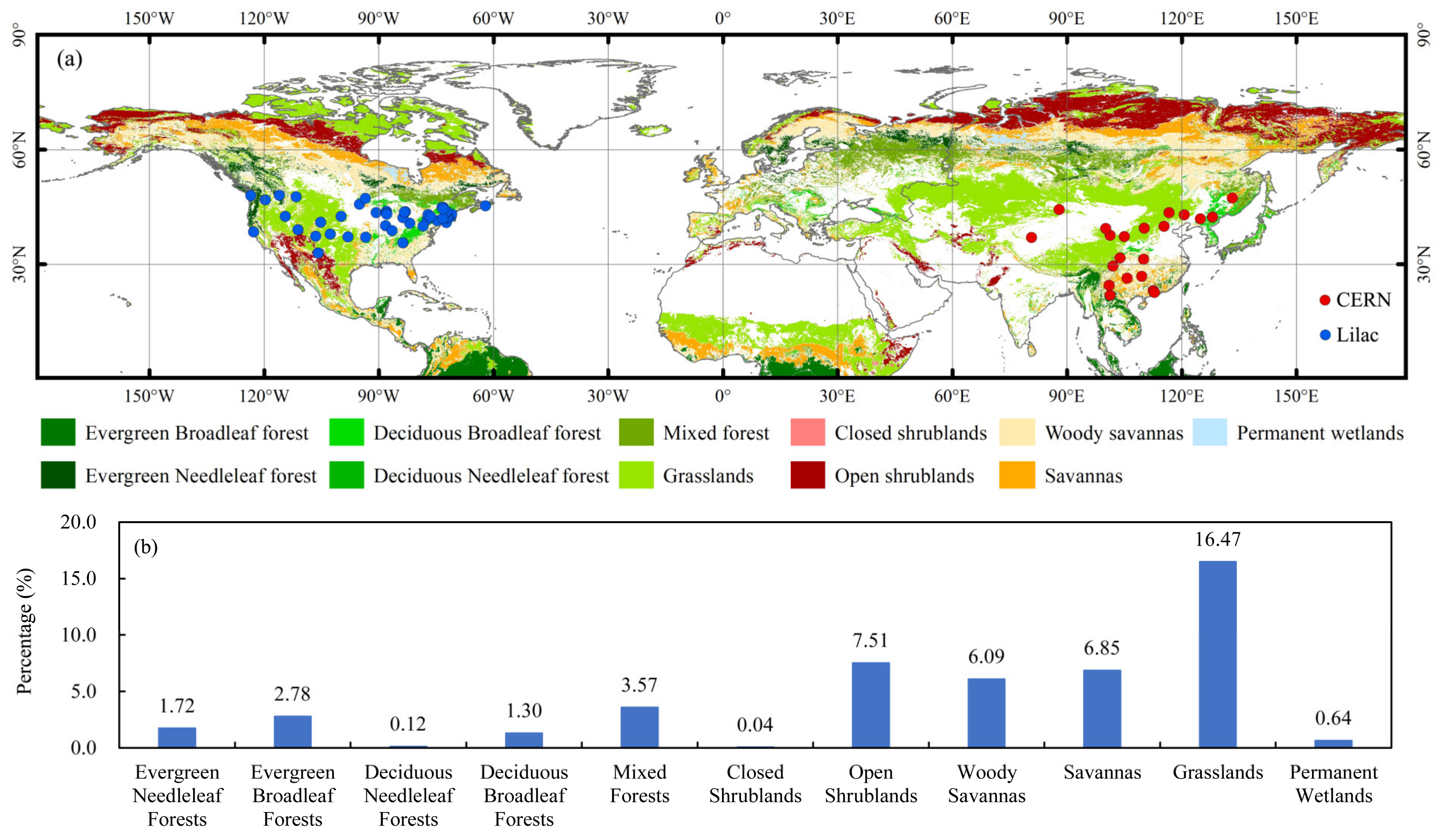
Ground-Vegetation-Phenology Observation Datasets

To verify the performance of MCD12Q2-C6 in capturing the distribution of the “real” SOS distribution over the NH, two ground-vegetation-phenology datasets were selected in this study, including the Chinese Ecosystem Research Network (CERN) and Lilac-leafing observations (Lilac).

The plant phenological-observation dataset of the CERN is the integration of plant phenological-observation data of more than 660 plant species [57]. In this study, 21 CERN stations all over China from 2003 to 2015 were used in the validation purpose.

The Lilac-leafing observations were collected across the continental United States from 1956 to 2014 for purple common lilac, a cloned lilac cultivar, and two cloned honeysuckle cultivars [15]. The Lilac-leafing observation dataset is unique in both its geographic and temporal coverage, with considerable potential to support additional research and applications [15]. Compared with other plants, lilac and honeysuckle respond predictably to air temperature and accumulated heat in a regionally coherent pattern. Large-scale, coordinated phenological monitoring of lilac and honeysuckle was initiated in the United States to supplement the use of weather observations in agricultural forecasts [15,58]. Therefore, in this study, 36 stations ranging from 2001 to 2014 across the United States were employed to validate the performance of the MCD12Q2-C6 SOS maps.

The distribution of the selected 68 ground-vegetation-phenology observations are displayed in Figure 1. Stations with incomplete records and with missing values over 75% of the temporal coverage were excluded in this study. In consideration of the definitional differences between the CERN and Lilac-leafing observations, the beginning of leaf unfolding in CERN and the first leafing date in Lilac were used as ground SOS observations.

2.2.2. Normalized-Difference Vegetation-Index Datasets

The SOS is generally negatively correlated with NDVI in spring. With earlier vegetation growth, the SOS advanced, resulting in a higher NDVI in spring. For cross-comparison with SOS maps derived from the MCD12Q2-C6, both the SPOT-VGT in 10-day temporal resolution from 2001 to 2014, at 950.469 m spatial resolution (http://free.vgt.vito.be/ (accessed on 15 December 2020)), and the GIMMS 3g in a half-month temporal resolution from 2001 to 2015, at 8 km spatial resolution [59], were used in this study. The primary input data for the SPOT-VGT and GIMMS 3g are totally independent of the MCD12Q2-C6, making the cross-comparison between the SOS from the MCD12Q2-C6 and the NDVI series from the GIMMS 3g and SPOT-VGT meaningful and credible.

2.2.3. Climate Variables

To attribute changes in the SOS to climate variability, the monthly averaged T_s and P_t derived from the fifth-generation European Center for Medium Range Weather Forecasts Reanalysis Land (ERA5-Land) datasets [55] were gridded at 0.1° spatial resolutions, and the S_c from the MOD10CM at a 0.05° spatial resolution [56] during 2001–2018, were used in this study.

2.2.4. Data Preparation

A summary of the gridded datasets is listed in

Table 1. Summary of datasets used in this study.

Variables	Datasets	Time Span	Temporal Resolution	Spatial Resolution	References/Sources
Land cover	MCD12C1 C6	2001–2018	Yearly	0.05°	Friedl and Sulla-Menashe [54]
SOS	MCD12Q2-C6	2001–2018	Yearly	500 m	Friedl et al. [1]
NDVI	SPOT-VGT	2001–2014	10-day	950.469 m	http://free.vgt.vito.be/ (accessed on 15 December 2020)
	GIMMS 3g	2001–2015	Half-month	0.083°	Tucker et al. [59]
Ts	ERA5-Land	2001–2018	Monthly	0.10°	Muñoz [55]
Pt
Sc	MCD10CM	2001–2018	Monthly	0.05°	Hall and Riggs [56]

. To match the spatial resolution of the datasets listed in Table 1, analysis was performed at a spatial resolution of 0.05°. For datasets with a spatial resolution finer than 0.05°, for example, the MCD12Q2-C6 and SPOT-VGT, we used “average” in the resampling process, which computed the average of all non-NODATA contributing pixels in the domain of our study. For datasets with a spatial resolution coarser than 0.05°, such as ERA5-Land, we used “cubic-spline” during the resampling process. Moreover, to match the temporal resolution of the MCD12Q2-C6 SOS, the NDVI series from the 10-day SPOT-VGT and the half-month GIMMS 3g, the monthly Ts and Pt from the RA5-Land, and the monthly Sc from MCD10CM, were aggregated to produce a March–April–May averaged spring series in the analysis, which computed the average value of each variable in March, April, and May for each year for the period 2001–2018.

2.3. Methods

2.3.1. Validation of the MCD12Q2-C6 SOS Using Ground Observations

Validating moderate-resolution satellite images by ground observations is a widely used approach in previous studies, such as Chen and Yang [43] and Hall et al. [60]. In this study, the root-mean-square error (RMSE) and bias were used as criteria to evaluate the differences between the MCD12Q2-C6 SOS and ground observations. The RMSE and the bias of the MCD12Q2-C6 to ground observations are expressed as Equations (1) and (2):

$$\mathrm{RMSE}=\sqrt{\frac{1}{\mathrm{n}}{\displaystyle \sum _{i=1}^{\mathrm{n}}{(G_i-M_i)}^2}}$$

(1)

$$\mathrm{Bias}=\frac{1}{\mathrm{n}}{\displaystyle \sum _{i=1}^{\mathrm{n}}(G_i-M_i)}$$

(2)

where M_i and G_i are the SOS value of sample i in the MCD12Q2-C6 and ground observations, respectively.

2.3.2. Changes Detection of the SOS

The temporal coverage of MCD12Q2-C6 was not long enough to produce meaningful changes when using the linear-regression approach for most of the grid cells within the study area. Therefore, we calculated the SOS changes by subtracting the five-year averaged SOS during 2014–2018 from the five-year averaged values in the earlier period 2001–2005, using Equation (3):

$$\Delta \mathrm{SOS}=\overline{{\mathrm{SOS}}_l}-\overline{{\mathrm{SOS}}_e}$$

(3)

where, $\overline{{\mathrm{SOS}}_l}$ is the five-year averaged SOS in the later period 2014–2018, and $\overline{{\mathrm{SOS}}_e}$ is the five-year averaged SOS in the earlier period 2001–2005.

2.3.3. Attribution Analysis

To consistently compare the contributions from T_s, P_t, and S_c to SOS changes, T_s, P_t, and S_c variations over the NH were converted into the standardized anomalies (z-score) series in the contribution analysis, using the mean and the standard deviation of each variable during 2001–2018 using Equation (4):

$$Z_x=\frac{x-{\mu }_x}{{\delta }_x}$$

(4)

where, μ_x is the mean of variable x, and σ_x is the standard deviation of variable x, in 2001–2018.

We hypothesized that the inter-annual variability of the SOS was co-determined by changes in T_s, P_t, and S_c. Therefore, we performed a multiple-linear-regression analysis using the SOS as the dependent variable and T_s, P_t, and S_c as the independent variables, which can be expressed by Equation (5):

$$\mathrm{SOS}=\alpha \times T_{\mathrm{s}}+\beta \times P_{\mathrm{t}}+\gamma \times S_{\mathrm{c}}+\epsilon$$

(5)

where, the regression coefficient α is the sensitivity of the SOS to surface air temperature T_s, which removed the effects of P_t and S_c on the SOS; the regression coefficient β is the sensitivity of the SOS to total precipitation P_t, which removed the effects of T_s and S_c on the SOS; and the regression coefficient γ is the sensitivity of the SOS to the snow-cover fraction S_c, which removed the effects of T_s and P_t on the SOS; and ε is the residual error, representing the contribution of unknown factors to the SOS, such as temperature sensitivity and photoperiod. Then, the contributions of T_s, P_t, and S_c to the SOS were reflected by the terms α × T_s, β × P_t, and γ × S_c, respectively.

Finally, the relative contributions of T_s, P_t, and S_c to SOS anomalies were confirmed using Equations (6)–(8), respectively.

$$C_T=\frac{|\alpha \times T_{\mathrm{s}}|}{|\alpha \times T_{\mathrm{s}}|+|\beta \times P_{\mathrm{t}}|+|\gamma \times S_{\mathrm{c}}|}$$

(6)

$$C_P=\frac{|\beta \times P_{\mathrm{t}}|}{|\alpha \times T_{\mathrm{s}}|+|\beta \times P_{\mathrm{t}}|+|\gamma \times S_{\mathrm{c}}|}$$

(7)

$$C_S=\frac{|\gamma \times S_{\mathrm{c}}|}{|\alpha \times T_{\mathrm{s}}|+|\beta \times P_{\mathrm{t}}|+|\gamma \times S_{\mathrm{c}}|}$$

(8)

where, C_T is the relative contributions of T_s to SOS anomalies, C_P is the relative contributions of P_t to SOS anomalies, and C_S is the relative contributions of S_c to SOS anomalies. This approach was used to quantify the contributions from climate variables to alpine vegetation green-up on the roof of the world [44], snow-cover phenology anomalies over the NH [61], and GPP anomalies in the Three North region of China [62].

3. Results

To explore the distribution and changes of the SOS over the NH, we first evaluated the performance of the MCD12Q2-C6 using the CERN and Lilac observations. Then, we explored the distribution and changes of the SOS over the NH during 2001–2018. Finally, we attributed SOS changes from T_s, P_t, and S_c in the corresponding period.

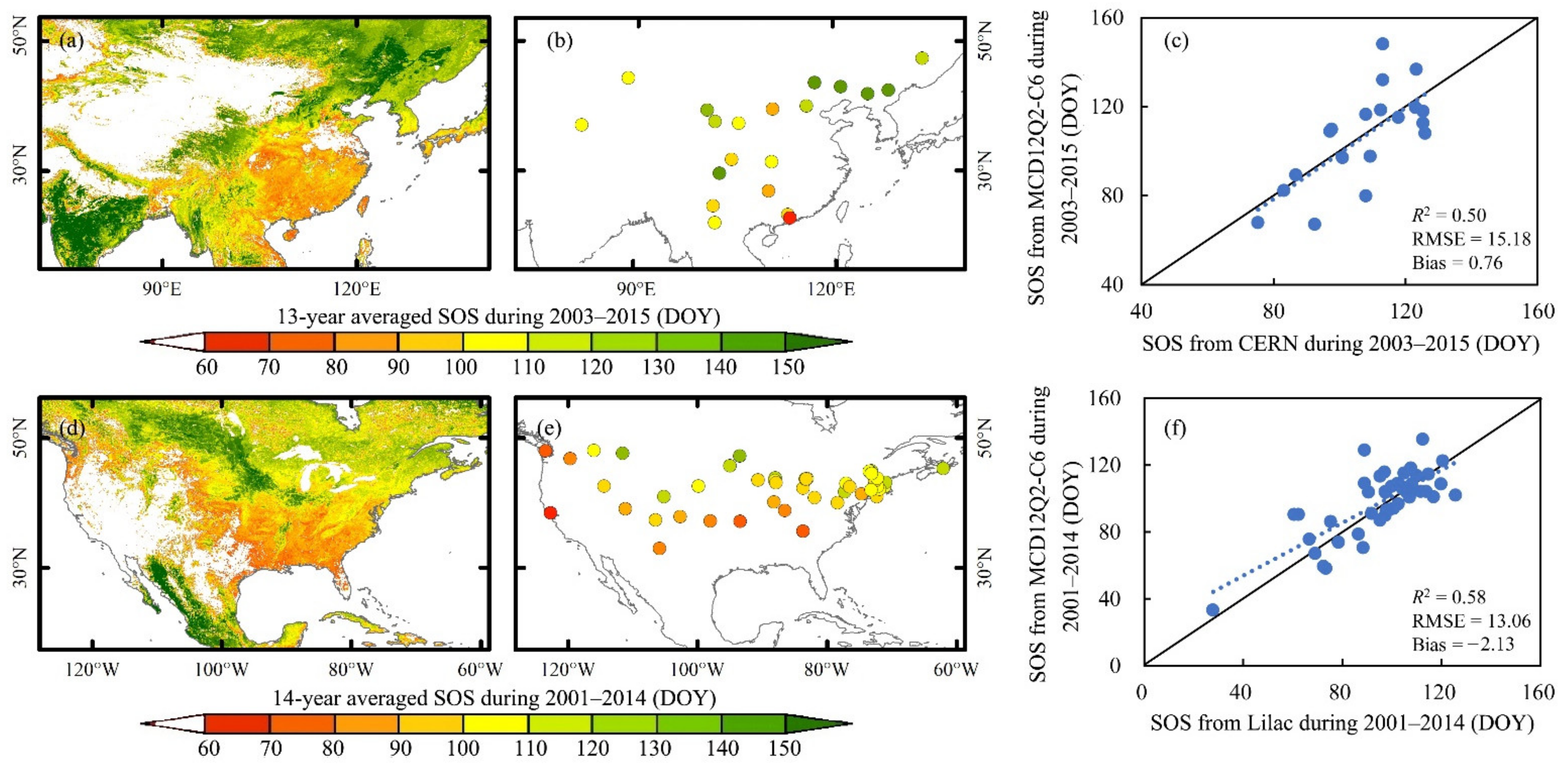
3.1. Performance of the MCD12Q2-C6 in SOS Monitoring over the NH

Subjected to the data availability, the comparisons between SOS maps from the MCD12Q2-C6 as well as CERN and Lilac were carried out during 2003–2015 and 2001–2014, respectively. The comparisons between the SOS from the MCD12Q2-C6 and two ground observations are displayed in Figure 2.

Similar to the SOS from the MCD12Q2-C6 over China (Figure 2a), there are clear latitudinal- and altitudinal-gradient patterns for the CERN SOS observations (Figure 2b), with an earlier SOS distributed in southeast China and a later SOS distributed in northern China. The scatter plots between the SOS from the MCD12Q2-C6 and CERN observations are presented in Figure 2c, in which the CERN SOS observations are consistent with the MCD12Q2-C6 SOS results; R² is 0.50 at the 95% confidence level. Meanwhile, the RMSE and bias between the MCD12Q2-C6 SOS and CERN observations were 15.18 and 0.76 days, respectively, during 2003–2015. The 14-year averaged SOS from the MCD12Q2-C6 over the United States (Figure 2d) and the Lilac observations (Figure 2e) during 2001–2014 also displayed similar spatial distributions. The linear-correlation coefficient, RMSE, and the bias between the MCD12Q2-C6 SOS and the Lilac observations for the period 2001–2014 were 0.58 (p < 0.05), 13.06, and −2.13 days, respectively.

Published study has proved that the raw in situ observations would give results that are highly dependent on the particular locations and reporting periods of the actual weather stations [63]. Therefore, results from ground observations only represent those accidental circumstances rather than yield any meaningful climatology information of the SOS. The large differences between the spatial representativeness of ground observations and satellite observations may lead to overestimation or underestimation issues in the comparison process, even though the MCD12Q2-C6 still captures the ground SOS distributions from the CERN (R² = 0.50, p < 0.05) and Lilac (R² = 0.58, p < 0.05). Thus, in the following context, we will use the MCD12Q2-C6 in the SOS-change analysis.

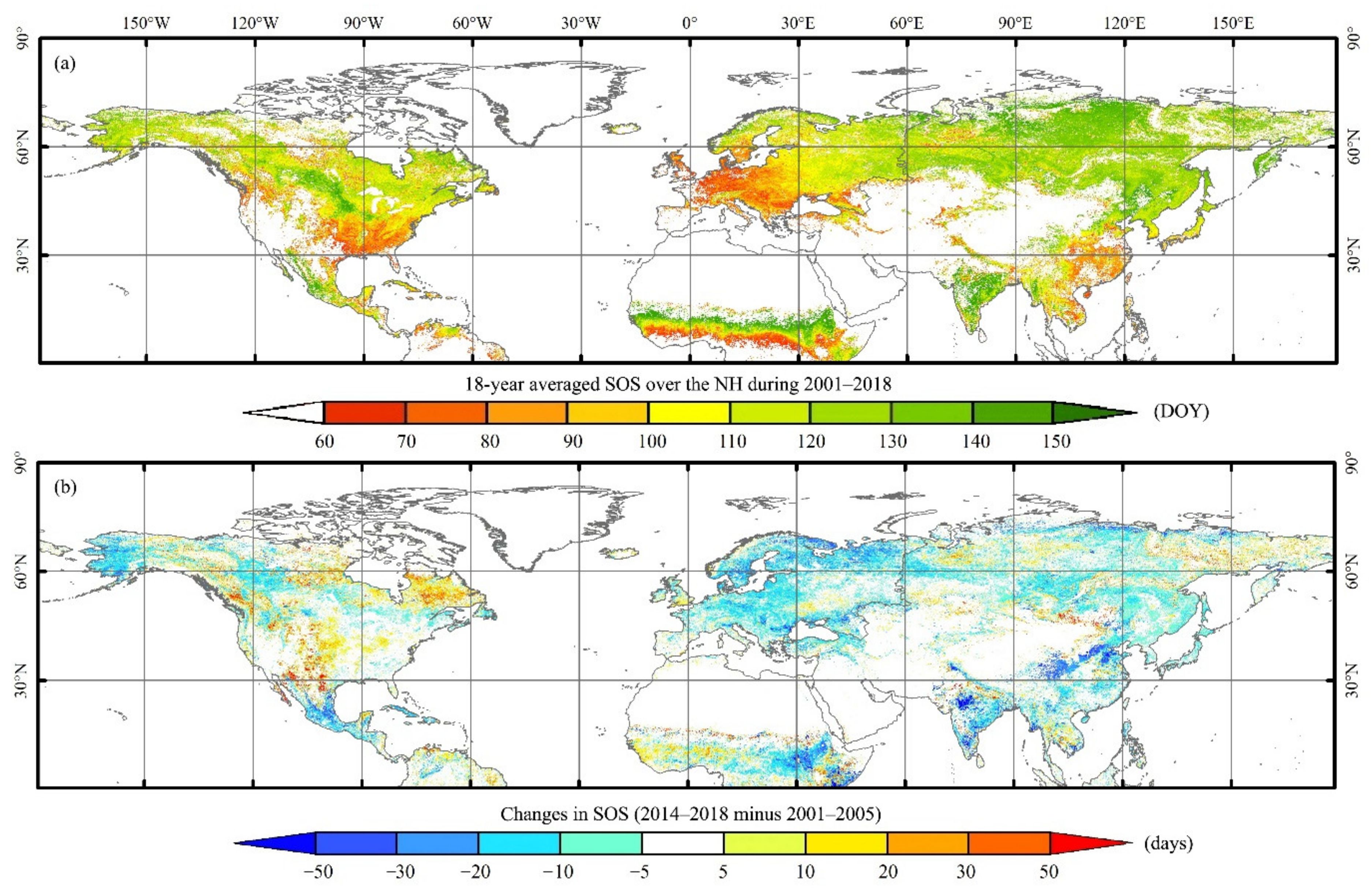
3.2. Distribution and Changes of the SOS over the NH between 2001 and 2018

The distribution of the 18-year averaged SOS over the NH from 2001 to 2018 and its associated changes are shown in Figure 3.

The mean SOS values from the MCD12Q2-C6 for the NH natural-vegetated regions during the 18-year period were 99 (±43) days of the year. As shown in Figure 3a, the vegetation became green earlier in the tropical and southern United States, southern Europe, and southeast China; however, it became green later in high Eurasia and the mountains in the central United States and northeast China. Moreover, the SOS over the NH was advanced by approximately 2.08 days on average, especially for Europe, China, and Alaska, USA, for 2001–2018 (Figure 3b).

The 18-year averaged SOS for 11 natural-vegetation types and the associated changes are displayed in Figure 4. Due to the spatial heterogeneity of T_s, P_t, and S_c distribution and the different responses of vegetation to temperature, precipitation, and snow-cover stress, there are large differences in SOS changes among the 11 natural-vegetation types (Figure 4). During 2001–2018, most of the natural-vegetation types displayed an earlier SOS, ranging from −10.66 days in closed shrublands to 0.58 days in permanent wetlands. Meanwhile, mixed forests presented a delayed SOS during the same period, with changes of 4.99 ± 0.13 days.

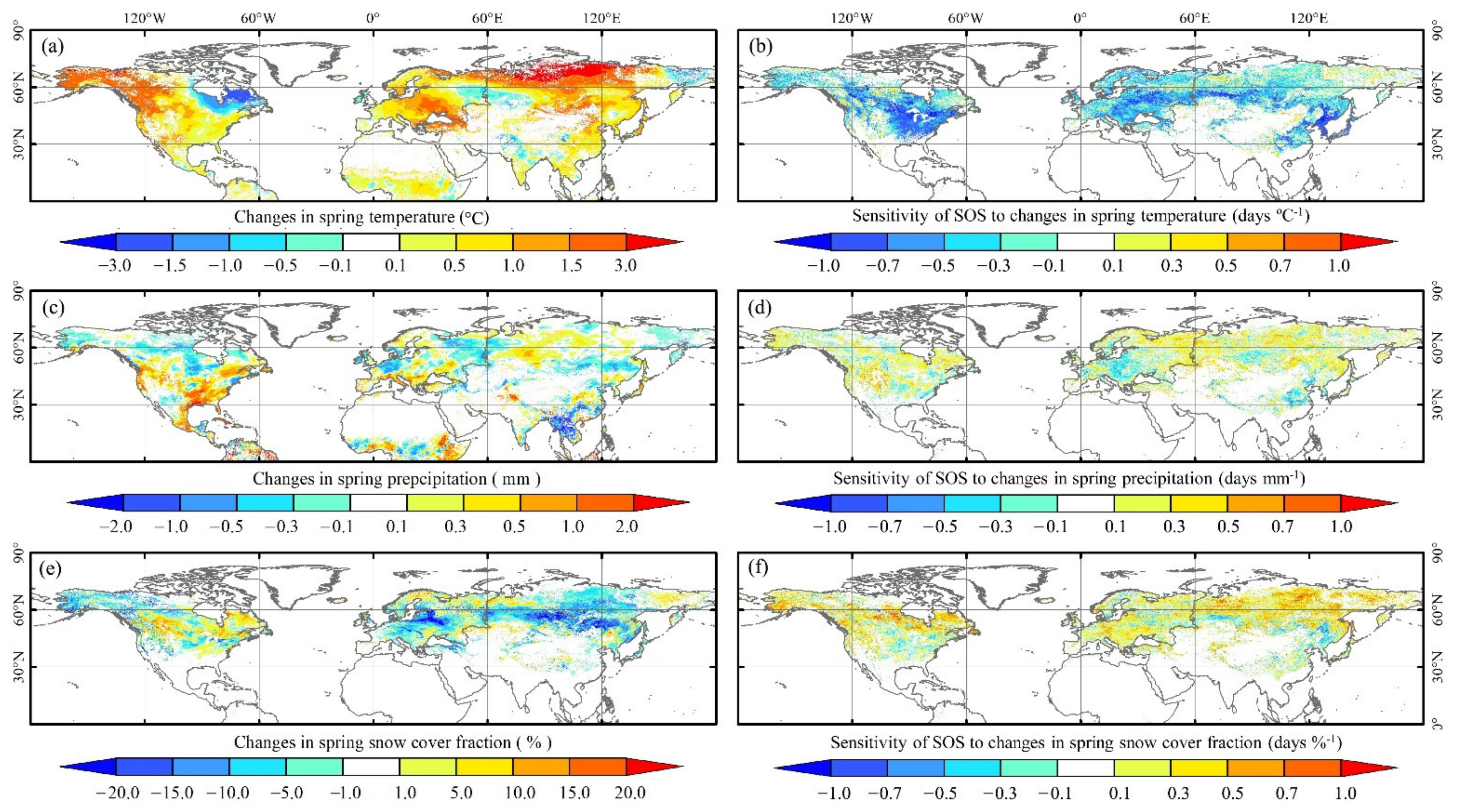
3.3. Attributions of SOS Changes over the NH

To attribute the changes in the SOS and further explore the response of different land-cover types to climate change, the present study calculated the sensitivity of the SOS to changes in spring T_s, P_t, and S_c over the NH for the period 2001–2018.

3.3.1. Sensitivity of the SOS to Changes in Temperature, Precipitation, and Snow Cover

The changes in spring T_s, P_t, and S_c, and the sensitivity of the SOS to T_s, P_t, and S_c variations over the NH from 2001 to 2018 are shown in Figure 5.

Driven by Arctic-amplification effects, where the warming magnitude at high latitudes is approximately two times higher than that at low latitudes [50], the T_s anomalies had a significant latitudinal difference from high to low latitudes over the NH from 2001 to 2018 (Figure 5a). Accompanying the T_s changes, P_t increased in the high latitudes of North America and western Russia as well as in Southeast Asia (Figure 5c) during 2001–2018. Meanwhile, driven by changes in the T_s and P_t, the S_c decreased significantly over the NH for the period 2001–2018, especially in Eurasia (Figure 5d).

The sensitivity analysis results from Equation (5) showed a negative sensitivity of the SOS to the spring T_s, of −1.21 (±0.34) days °C⁻¹ across the NH from 2001 to 2018 (Figure 5a). Therefore, as the T_s increased by 1 °C, the SOS would be advanced by 1.21 (±0.34) days. In addition, areas with the most positive sensitivity of the SOS to T_s were distributed in the eastern United States as well as central and eastern Asia. The sensitivity of the SOS to the S_c was estimated as 0.62 (±0.29) days %⁻¹; therefore, as the S_c increased by 1%, the SOS would be delayed by 0.62 (±0.29) days. Compared with the S_c, the positive sensitivity of the SOS to P_t was smaller at 0.24 (±0.21) days mm⁻¹ over the NH between 2001 and 2018.

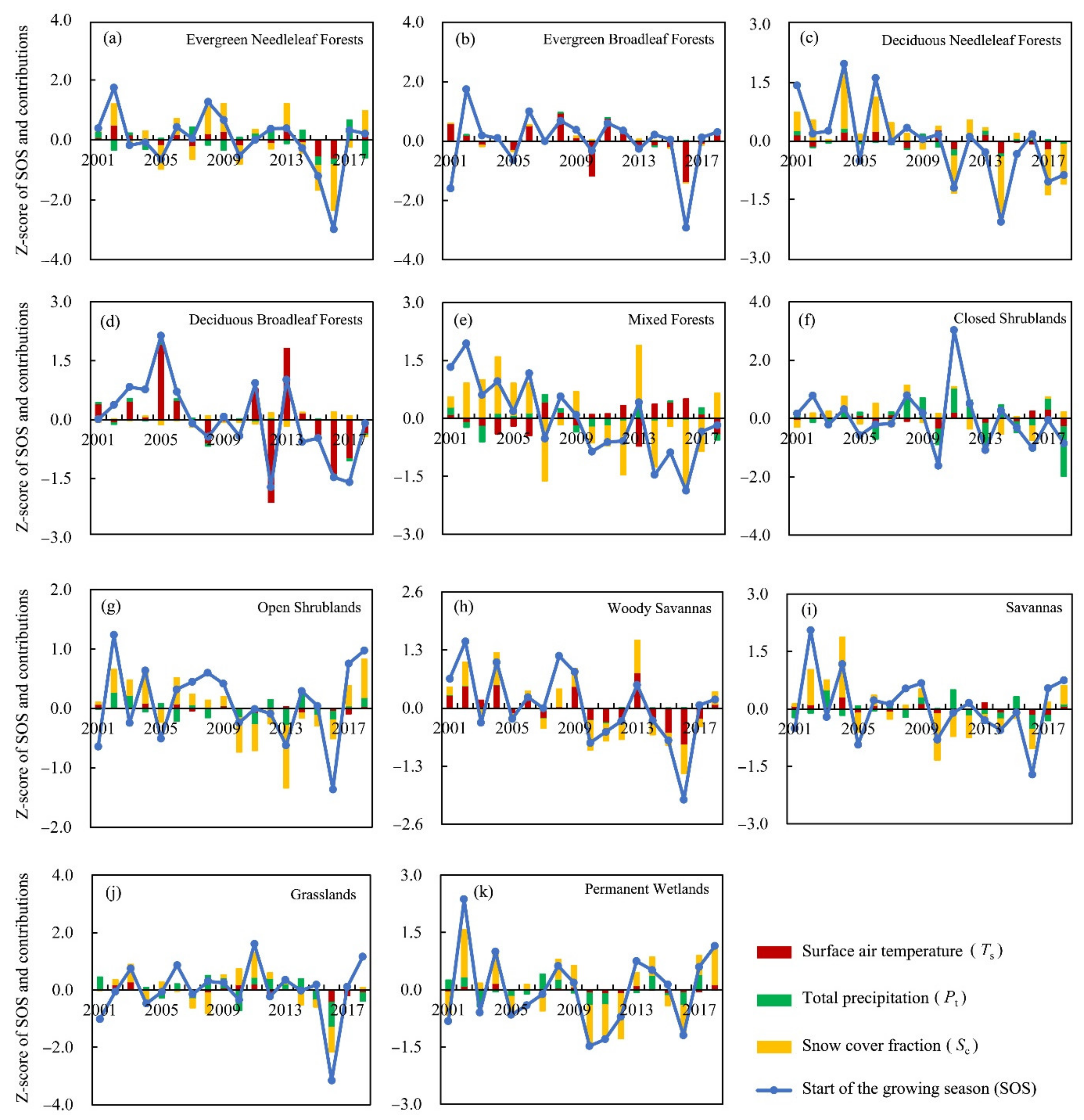
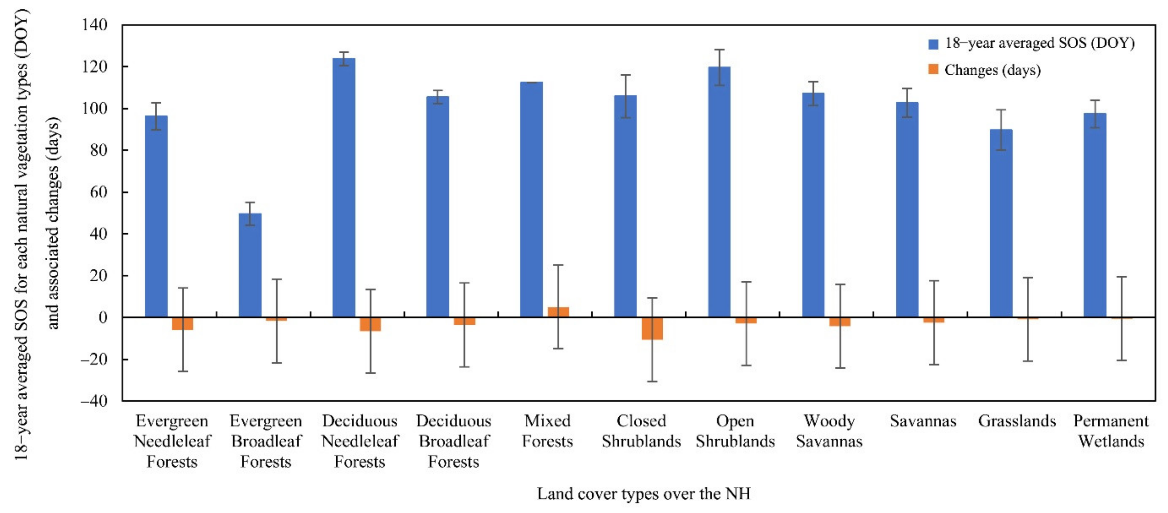
3.3.2. Attribution of SOS Anomalies for Different Land-Cover Types

To explore the large differences in SOS anomalies among the NH between 2001 and 2018 (Figure 4), the present study further calculated the sensitivity of the SOS to T_s, P_t, and S_c for the 11 natural-land-cover types (

Table 2. Sensitivity of spring SOS to changes in T_s, P_t, and S_c.

Land Cover Types	Ts	Pt	Sc
Evergreen needleleaf forests	−0.3025 (**)	0.3188	0.6906 (**)
Evergreen broadleaf forests	−0.5954 (**)	0.0006	0.0242
Deciduous needleleaf forests	−0.1854 (**)	0.0848	0.7476 (**)
Deciduous broadleaf forests	−0.9843 (**)	−0.0369	−0.0837
Mixed forests	0.3528 (**)	0.1867	1.0522 (**)
Closed shrublands	0.1914	−0.6259 (**)	0.3070
Open shrublands	−0.0550	0.1710	0.4324 (**)
Woody savannas	−0.4214 (**)	0.0098	0.4309 (**)
Savannas	−0.1406	−0.2374	0.6098 (**)
Grasslands	−0.1736 (*)	−0.3860	0.4374 (**)
Permanent wetlands	−0.0913 (**)	0.2642 (*)	0.7306 (**)

Notes: one and two asterisks denote significance at the 95% and 99% levels, respectively. Others are not significant at the 95% level.

). The resulting contributions from T_s, P_t, and S_c to SOS anomalies for the 11 natural-vegetation types over the NH during 2001–2018 are shown in Figure 6.

Compared with the P_t and S_c, the T_s was the dominating factor for SOS changes for most land-cover types, except for closed shrublands, open shrublands, and savannas, during 2001–2018. The maximum sensitivity of the SOS to T_s occurred in deciduous broadleaf forests, with −0.98 days °C⁻¹. Except for the negative sensitivity of the SOS to T_s, mixed forests and closed shrublands displayed positive sensitivity in the same period. The S_c was the second driving factor of SOS anomalies over the NH. With the increase in S_c, the SOS was delayed, and vice versa.

As shown in Table 2, the sensitivity of the SOS to S_c was up to 1.05 days %⁻¹, 0.75 days %⁻¹, and 0.73 days %⁻¹ for mixed forests, deciduous needleleaf forests, and permanent wetlands, respectively, between 2001 and 2018. Meanwhile, SOS anomalies in evergreen broadleaf forests, deciduous broadleaf forests, and closed shrublands were not influenced by S_c changes during the same period. Compared with the T_s and S_c, the P_t was less important in SOS anomalies for most land-cover types, except for closed shrublands and permanent wetlands. The competing effects between T_s and P_t are complex in climate change studies, especially during spring. Although changes in the SOS and P_t were statistically significant at the 95% confidence level for closed shrublands and permanent wetlands, they moved in different directions. For closed shrublands, the SOS was negatively correlated with the P_t at −0.62 days mm⁻¹, whereas the value was 0.26 days mm⁻¹ for permanent wetlands.

The resulting contributions from T_s, P_t, and S_c to SOS anomalies were significantly different for different land cover types. However, changes in the SOS can be well-represented by T_s, P_t, and S_c, using the multiple-linear-regression equation with different coefficients. The T_s largely explained the SOS anomalies in evergreen broadleaf forests (Figure 6b), deciduous broadleaf forests (Figure 6d), and woody savannas (Figure 6h). Meanwhile, the S_c dominated the SOS anomalies in evergreen needleleaf forests (Figure 6a), deciduous needleleaf forests (Figure 6c), grasslands (Figure 6j), and permanent wetlands (Figure 6k). However, the SOS anomalies in mixed forests were not well represented by the changes in T_s, P_t, and S_c. Further studies are required done to determine the reasons for the SOS anomalies in mixed forests in the NH.

4. Discussion

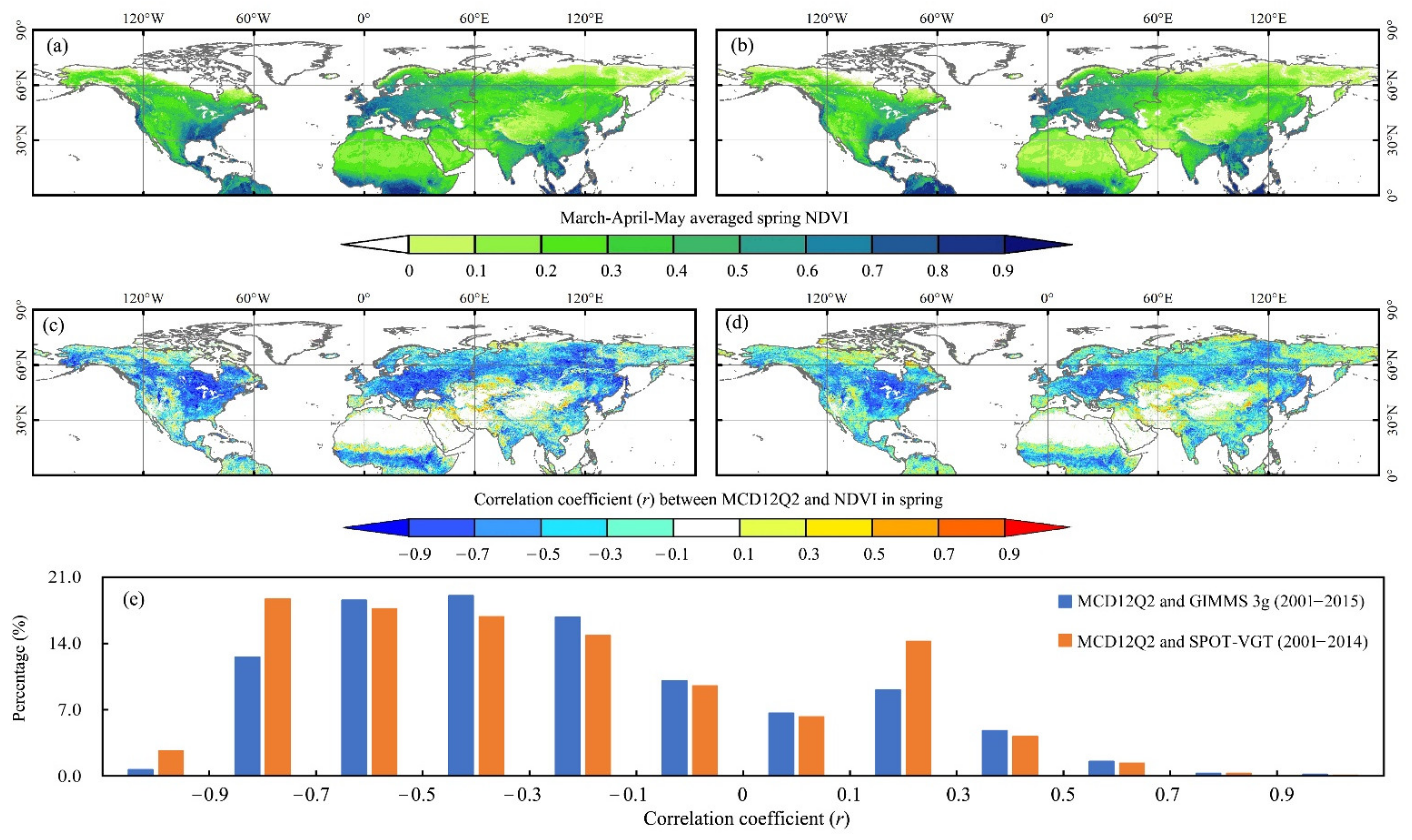
4.1. Consistency between the MCD12Q2-C6 SOS and Individual Spring NDVI Series

Subjected to the temporal coverage of the SPOT-VGT and GIMMS 3g, the cross-comparisons between the MCD12Q2-C6 SOS and individual spring NDVI series from the SPOT-VGT and GIMMS 3g were performed for the overlapping periods 2001–2014 and 2001–2015, respectively. The 14-year averaged spring NDVI from the SPOT-VGT during 2001–2014 and the 15-year averaged spring NDVI from the GIMMS 3g during 2001–2015 are shown in (Figure 7a,b). The linear-correlation coefficients between the spring NDVI from the SPOT-VGT and the SOS during 2001–2014, and the comparable results from the GIMMS 3g for the period 2001–2015, are displayed in Figure 7c,d, respectively.

As shown in (Figure 7a,b), there are clear latitudinal and regional differences in the distribution of the spring NDVI over the NH, with a higher NDVI distributed in tropical regions and a lower NDVI distributed in arid and semi-arid regions as well as the landmasses around the Arctic. A histogram of correlation coefficients between the SOS from the MCD12Q2-C6 and the spring NDVI series from the SPOT-VGT and GIMMS 3g is presented in Figure 7e. Limited by the systematic bias of the different datasets, the SOS changes were negatively correlated with the spring NDVI from the SPOT-VGT from 2001 to 2014 by over 80% of the study area. In comparison, the results were 78% for the spring NDVI from the GIMMS 3g during 2001–2015.

4.2. Uncertainty Analysis

Compared with ground observation, the satellite-retrieved vegetation-phenology datasets are a priority in large-scale SOS studies. Although ground stations provide “real” vegetation-phenology observations, their distribution and spatial representation are limited over the NH.

Except for the spatial distribution of the SOS, this study also explored the contribution of T_s, P_t, and S_c to SOS changes over the NH from 2001 to 2018, which clarifies the driving factors of the SOS at a continental scale. Compared with other factors, T_s, P_t, and S_c are basic and comprehensive variables. However, except for T_s, P_t, and S_c, changes in temperature sensitivity [7,49] and photoperiod [47,48] also contributed to SOS changes. To explore a general sensitivity of the SOS to changes in T_s, P_t, and S_c, the present study produced a MAM-averaged spring T_s in the attribution analysis, which combined the changes in T_s and temperature sensitivity in the attribution analysis. Moreover, due to the lack of a high-quality gridded-photoperiod dataset, this study excluded the photoperiod from the attribution analysis. Since changes in the SOS are acclimation-adjustment processes rather than instantaneous feedback, the individual effects of the temperature sensitivity and photoperiod on the SOS should be taken into consideration in future studies.

5. Conclusions

Understanding the response of spring-vegetation phenology to climatic factors is important for projecting the land-climate interactions of ecosystems under climate change. With accelerated surface warming, snow-cover reduction, and permafrost thawing over the NH in the past decades, it is vital to explore the distribution and attribution of the SOS with the latest observations. Based on satellite-retrieved vegetation-phenology datasets, ground observations, and several auxiliary datasets, this study estimated the performance of the MCD12Q2-C6 in SOS monitoring, quantified the spatial distribution of the SOS over the NH, and explored its attributions for the period 2001–2018.

Compared with other satellite-retrieved dynamic-vegetation dataset, the MCD12Q2-C6 constitutes consistent and objective vegetation phenology metrics derived from satellite data with a higher spatial resolution than that of MEaSUREs VIP and a better methodological approach than that of the MCD12Q2-C5. The validation results using the CERN and Lilac vegetation-phenology observations proved the fitness of the MCD12Q2-C6 in capturing the “real” distribution of the SOS over the NH. The linear-correlation coefficient between the SOS from the MCD12Q2-C6 and CERN was 0.50 (p < 0.05) during 2003–2015. Meanwhile, the comparable result between the SOS from the MCD12Q2-C6 and Lilac observations was 0.58 (p < 0.05) during 2001–2014. In addition, changes in the SOS from the MCD12Q2-C6 were explored and further cross-compared with two independent spring NDVI series. The SOS is generally negatively correlated with the NDVI in spring. With earlier vegetation growth, the SOS advanced, resulting in a higher NDVI in spring. The SOS calculated from the MCD12Q2-C6 was negatively correlated with a spring NDVI from the SPOT-VGT during 2001–2014, for over 80% of the study area. Meanwhile, the result was 78% for a spring NDVI from the GIMMS 3g during 2001–2015.

Using the MCD12Q2-C6 and several ancillary datasets, this study also explored changes in the SOS and its attribution factors. Evidence from the MCD12Q2-C6 pointed out that the SOS was advanced by 2.08 days on average over the NH for the period of 2001–2018, especially for Europe, China, and Alaska, United States. In addition, the detailed-sensitivity analysis showed that the increased T_s (−1.21 ± 0.34 days °C⁻¹) and reduced SCF (0.62 ± 0.29 days%⁻¹) were the key driving factors of the observed SOS changes over the NH during 2001–2018. In addition, attribution of SOS anomalies for different land-cover types pointed that the maximum sensitivity of the SOS to T_s (−0.98 days °C⁻¹) and S_c (1.05 days %⁻¹) occurred in deciduous broadleaf forests and mixed forests, respectively. Compared with the T_s and S_c, the role of the P_t was minor in dominating the spring-vegetation-phenology changes during the same period.

Compared with previous studies, the present study mapped the climatology of the SOS using the latest MCD12Q2-C6 with the best available spatial resolution, detected changes in the SOS, and explored the response of the SOS to climate change among different land-cover types over the NH between 2001 and 2018, which would be helpful for continental, regional, and local spring-vegetation studies. The present study also explored the different mechanisms controlling SOS anomalies among the 11 natural-vegetation types, which is benefit for large-scale climate-change studies. Climate projections suggest that surface temperature increase [64] and snow-cover decrease [65] will continue over the next several decades. Therefore, the investigation of the SOS in climate projections should consider the land-cover types. However, subject to the lack of a continent-scale satellite-retrieved vegetation-phenology dataset with finer spatial resolution and limited distribution of ground-vegetation-phenology observations, the accuracy evaluation of the MCD12Q2-C6 is still insufficient at present. With the development of harmonized Landsat 8 and Sentinel-2 imagery [33] at a 30 m spatial resolution, a comprehensive estimation of the MCD12Q2-C6 is expected in the future.

References

1. Friedl, M.; Gray, J.; Sulla-Menashe, D. MCD12Q2 MODIS/Terra+Aqua Land Cover Dynamics Yearly L3 Global 500m SIN Grid V006. NASA EOSDIS Land Processes Distributed Active Archive Center. 2019. Available online: https://lpdaac.usgs.gov/products/mcd12q2v006/ (accessed on 15 September 2021).
2. Ivits, E.; Cherlet, M.; Mehl, W.; Sommer, S. Ecosystem functional units characterized by satellite observed phenology and productivity gradients: A case study for Europe. Ecol. Indic. 2013, 27, 17–28. [Google Scholar] [CrossRef]
3. Lan, X.; Li, Y.; Shao, R.; Chen, X.; Lin, K.; Cheng, L.; Gao, H.; Liu, Z. Vegetation controls on surface energy partitioning and water budget over China. J. Hydrol. 2020, 600, 125646. [Google Scholar] [CrossRef]
4. Joiner, J.; Yoshida, Y.; Vasilkov, A.P.; Schaefer, K.; Jung, M.; Guanter, L.; Zhang, Y.; Garrity, S.; Middleton, E.M.; Huemmrich, K.F.; et al. The seasonal cycle of satellite chlorophyll fluorescence observations and its relationship to vegetation phenology and ecosystem atmosphere carbon exchange. Remote Sens. Environ. 2014, 152, 375–391. [Google Scholar] [CrossRef] [Green Version]
5. Peñuelas, J.; Rutishauser, T.; Filella, I. Phenology Feedbacks on Climate Change. Science 2009, 324, 887–888. [Google Scholar] [CrossRef] [Green Version]
6. Loranty, M.M.; Berner, L.T.; Goetz, S.J.; Jin, Y.; Randerson, J.T. Vegetation controls on northern high latitude snow-albedo feedback: Observations and CMIP5 model simulations. Glob. Chang. Biol. 2014, 20, 594–606. [Google Scholar] [CrossRef]
7. Wang, C.; Cao, R.; Chen, J.; Rao, Y.; Tang, Y. Temperature sensitivity of spring vegetation phenology correlates to within-spring warming speed over the Northern Hemisphere. Ecol. Indic. 2015, 50, 62–68. [Google Scholar] [CrossRef]
8. Richardson, A.D.; Anderson, R.S.; Arain, M.A.; Barr, A.G.; Bohrer, G.; Chen, G.; Chen, J.M.; Ciais, P.; Davis, K.J.; Desai, A.R.; et al. Terrestrial biosphere models need better representation of vegetation phenology: Results from the North American Carbon Program Site Synthesis. Glob. Chang. Biol. 2012, 18, 566–584. [Google Scholar] [CrossRef] [Green Version]
9. Zhao, D.; Li, N.; Zare, E.; Wang, J.; Triantafilis, J. Mapping cation exchange capacity using a quasi-3d joint inversion of EM38 and EM31 data. Soil Tillage Res. 2020, 200, 104618. [Google Scholar] [CrossRef]
10. Zhao, D.; Zhao, X.; Khongnawang, T.; Arshad, M.; Triantafilis, J. A Vis-NIR Spectral Library to Predict Clay in Australian Cotton Growing Soil. Soil Sci. Soc. Am. J. 2018, 82, 1347–1357. [Google Scholar] [CrossRef]
11. Goetz, S.J.; Bunn, A.G.; Fiske, G.J.; Houghton, R.A. Satellite-observed photosynthetic trends across boreal North America associated with climate and fire disturbance. Proc. Natl. Acad. Sci. USA 2005, 102, 13521–13525. [Google Scholar] [CrossRef] [Green Version]
12. Val Martin, M.; Heald, C.L.; Arnold, S.R. Coupling dry deposition to vegetation phenology in the Community Earth System Model: Implications for the simulation of surface O3. Geophys. Res. Lett. 2014, 41, 2988–2996. [Google Scholar] [CrossRef]
13. Lorenz, R.; Davin, E.L.; Lawrence, D.M.; Stöckli, R.; Seneviratne, S.I. How Important is Vegetation Phenology for European Climate and Heat Waves? J. Clim. 2013, 26, 10077–10100. [Google Scholar] [CrossRef] [Green Version]
14. Donnelly, A.; Yu, R. The rise of phenology with climate change: An evaluation of IJB publications. Int. J. Biometeorol. 2017, 61, 29–50. [Google Scholar] [CrossRef]
15. Rosemartin, A.H.; Denny, E.G.; Weltzin, J.F.; Lee Marsh, R.; Wilson, B.E.; Mehdipoor, H.; Zurita-Milla, R.; Schwartz, M.D. Lilac and honeysuckle phenology data 1956–2014. Sci. Data 2015, 2, 150038. [Google Scholar] [CrossRef] [PubMed] [Green Version]
16. Schwartz, M.D.; Ahas, R.; Aasa, A. Onset of spring starting earlier across the Northern Hemisphere. Glob. Chang. Biol. 2006, 12, 343–351. [Google Scholar] [CrossRef]
17. Jeong, S.-J.; Ho, C.-H.; Gim, H.-J.; Brown, M.E. Phenology shifts at start vs. end of growing season in temperate vegetation over the Northern Hemisphere for the period 1982–2008. Glob. Chang. Biol. 2011, 17, 2385–2399. [Google Scholar] [CrossRef]
18. Wang, L.; Fensholt, R. Temporal Changes in Coupled Vegetation Phenology and Productivity are Biome-Specific in the Northern Hemisphere. Remote Sens. 2017, 9, 1277. [Google Scholar] [CrossRef] [Green Version]
19. Bi, J.; Xu, L.; Samanta, A.; Zhu, Z.; Myneni, R. Divergent Arctic-Boreal Vegetation Changes between North America and Eurasia over the Past 30 Years. Remote Sens. 2013, 5, 2093–2112. [Google Scholar] [CrossRef] [Green Version]
20. Elmendorf, S.C.; Henry, G.H.R.; Hollister, R.D.; Björk, R.G.; Boulanger-Lapointe, N.; Cooper, E.J.; Cornelissen, J.H.C.; Day, T.A.; Dorrepaal, E.; Elumeeva, T.G.; et al. Plot-scale evidence of tundra vegetation change and links to recent summer warming. Nat. Clim. Chang. 2012, 2, 453–457. [Google Scholar] [CrossRef]
21. Høgda, K.; Tømmervik, H.; Karlsen, S. Trends in the Start of the Growing Season in Fennoscandia 1982–2011. Remote Sens. 2013, 5, 4304–4318. [Google Scholar] [CrossRef] [Green Version]
22. Fu, Y.H.; Piao, S.; Op de Beeck, M.; Cong, N.; Zhao, H.; Zhang, Y.; Menzel, A.; Janssens, I.A. Recent spring phenology shifts in western Central Europe based on multiscale observations. Glob. Ecol. Biogeogr. 2014, 23, 1255–1263. [Google Scholar] [CrossRef]
23. Bogaert, J.; Zhou, L.; Tucker, C.J.; Myneni, R.B.; Ceulemans, R. Evidence for a persistent and extensive greening trend in Eurasia inferred from satellite vegetation index data. J. Geophys. Res. Atmos. 2002, 107, ACL 4-1–ACL 4-14. [Google Scholar] [CrossRef]
24. Menzel, A.; Fabian, P. Growing season extended in Europe. Nature 1999, 397, 659. [Google Scholar] [CrossRef]
25. Wang, X.; Gao, Q.; Wang, C.; Yu, M. Spatiotemporal patterns of vegetation phenology change and relationships with climate in the two transects of East China. Glob. Ecol. Conserv. 2017, 10, 206–219. [Google Scholar] [CrossRef]
26. Yang, B.; He, M.; Shishov, V.; Tychkov, I.; Vaganov, E.; Rossi, S.; Ljungqvist, F.C.; Bräuning, A.; Grießinger, J. New perspective on spring vegetation phenology and global climate change based on Tibetan Plateau tree-ring data. Proc. Natl. Acad. Sci. USA 2017, 114, 6966–6971. [Google Scholar] [CrossRef] [PubMed] [Green Version]
27. Wang, C.; Guo, H.; Zhang, L.; Liu, S.; Qiu, Y.; Sun, Z. Assessing phenological change and climatic control of alpine grasslands in the Tibetan Plateau with MODIS time series. Int. J. Biometeorol. 2015, 59, 11–23. [Google Scholar] [CrossRef]
28. Zhang, G.; Zhang, Y.; Dong, J.; Xiao, X. Green-up dates in the Tibetan Plateau have continuously advanced from 1982 to 2011. Proc. Natl. Acad. Sci. USA 2013, 110, 4309–4314. [Google Scholar] [CrossRef] [Green Version]
29. Konrad, W.; Karen, S.; Graham, M.v.; Sally, A. Remotely sensed vegetation phenology for describing and predicting the biomes of South Africa. Appl. Veg. Sci. 2011, 14, 49–66. [Google Scholar]
30. Ganguly, S.; Friedl, M.A.; Tan, B.; Zhang, X.; Verma, M. Land surface phenology from MODIS: Characterization of the Collection 5 global land cover dynamics product. Remote Sens. Environ. 2010, 114, 1805–1816. [Google Scholar] [CrossRef] [Green Version]
31. Didan, K.; Barreto, A. NASA MEaSUREs Vegetation Index and Phenology (VIP) Phenology EVI2 Yearly Global 0.05Deg CMG. NASA EOSDIS Land Processes Distributed Active Archive Center. 2016. Available online: https://lpdaac.usgs.gov/news/nasa-vegetation-index-and-phenology-vip-data-released/ (accessed on 15 September 2020).
32. Zhang, X.; Liu, L.; Liu, Y.; Jayavelu, S.; Wang, J.; Moon, M.; Henebry, G.M.; Friedl, M.A.; Schaaf, C.B. Generation and evaluation of the VIIRS land surface phenology product. Remote Sens. Environ. 2018, 216, 212–229. [Google Scholar] [CrossRef]
33. Bolton, D.K.; Gray, J.M.; Melaas, E.K.; Moon, M.; Eklundh, L.; Friedl, M.A. Continental-scale land surface phenology from harmonized Landsat 8 and Sentinel-2 imagery. Remote Sens. Environ. 2020, 240, 111685. [Google Scholar] [CrossRef]
34. Araya, S.; Lyle, G.; Lewis, M.; Ostendorf, B. Phenologic metrics derived from MODIS NDVI as indicators for Plant Available Water-holding Capacity. Ecol. Indic. 2016, 60, 1263–1272. [Google Scholar] [CrossRef]
35. Zhumanova, M.; Mönnig, C.; Hergarten, C.; Darr, D.; Wrage-Mönnig, N. Assessment of vegetation degradation in mountainous pastures of the Western Tien-Shan, Kyrgyzstan, using eMODIS NDVI. Ecol. Indic. 2018, 95, 527–543. [Google Scholar] [CrossRef]
36. He, Y.; Bo, Y.; de Jong, R.; Li, A.; Zhu, Y.; Cheng, J. Comparison of vegetation phenological metrics extracted from GIMMS NDVIg and MERIS MTCI data sets over China. Int. J. Remote Sens. 2015, 36, 300–317. [Google Scholar] [CrossRef]
37. Julien, Y.; Sobrino, J. A Global land surface phenology trends from GIMMS database. Int. J. Remote Sens. 2009, 30, 3495–3513. [Google Scholar] [CrossRef] [Green Version]
38. Wang, X.; Xiao, J.; Li, X.; Cheng, G.; Ma, M.; Zhu, G.; Altaf Arain, M.; Andrew Black, T.; Jassal, R.S. No trends in spring and autumn phenology during the global warming hiatus. Nat. Commun. 2019, 10, 2389. [Google Scholar] [CrossRef]
39. Fu, Y.H.; Zhao, H.; Piao, S.; Peaucelle, M.; Peng, S.; Zhou, G.; Ciais, P.; Huang, M.; Menzel, A.; Penuelas, J.; et al. Declining global warming effects on the phenology of spring leaf unfolding. Nature 2015, 526, 104–107. [Google Scholar] [CrossRef] [Green Version]
40. Forkel, M.; Migliavacca, M.; Thonicke, K.; Reichstein, M.; Schaphoff, S.; Weber, U.; Carvalhais, N. Codominant water control on global interannual variability and trends in land surface phenology and greenness. Glob. Chang. Biol. 2015, 21, 3414–3435. [Google Scholar] [CrossRef]
41. Ying, H.; Zhang, H.; Zhao, J.; Shan, Y.; Zhang, Z.; Guo, X.; Rihan, W.; Deng, G. Effects of spring and summer extreme climate events on the autumn phenology of different vegetation types of Inner Mongolia, China, from 1982 to 2015. Ecol. Indic. 2020, 111, 105974. [Google Scholar] [CrossRef]
42. Ren, S.; Li, Y.; Peichl, M. Diverse effects of climate at different times on grassland phenology in mid-latitude of the Northern Hemisphere. Ecol. Indic. 2020, 113, 106260. [Google Scholar] [CrossRef]
43. Chen, X.; Yang, Y. Observed earlier start of the growing season from middle to high latitudes across the Northern Hemisphere snow-covered landmass for the period 2001–2014. Environ. Res. Lett. 2020, 15, 034042. [Google Scholar] [CrossRef]
44. Chen, X.; An, S.; Inouye, D.W.; Schwartz, M.D. Temperature and snowfall trigger alpine vegetation green-up on the world’s roof. Glob. Chang. Biol. 2015, 21, 3635–3646. [Google Scholar] [CrossRef] [PubMed]
45. Krishnaswamy, J.; John, R.; Joseph, S. Consistent response of vegetation dynamics to recent climate change in tropical mountain regions. Glob. Chang. Biol. 2014, 20, 203–215. [Google Scholar] [CrossRef]
46. Yin, C.; Yang, Y.; Yang, F.; Chen, X.; Xin, Y.; Luo, P. Diagnose the dominant climate factors and periods of spring phenology in Qinling Mountains, China. Ecol. Indic. 2021, 131, 108211. [Google Scholar] [CrossRef]
47. Adole, T.; Dash, J.; Rodriguez-Galiano, V.; Atkinson, P.M. Photoperiod controls vegetation phenology across Africa. Commun. Biol. 2019, 2, 391. [Google Scholar] [CrossRef] [PubMed] [Green Version]
48. Meng, L.; Zhou, Y.; Gu, L.; Richardson, A.D.; Penuelas, J.; Fu, Y.; Wang, Y.; Asrar, G.R.; De Boeck, H.J.; Mao, J.; et al. Photoperiod decelerates the advance of spring phenology of six deciduous tree species under climate warming. Glob. Chang. Biol. 2021, 27, 2914–2927. [Google Scholar] [CrossRef] [PubMed]
49. Shen, M.; Tang, Y.; Chen, J.; Yang, X.; Wang, C.; Cui, X.; Yang, Y.; Han, L.; Li, L.; Du, J.; et al. Earlier-season vegetation has greater temperature sensitivity of spring phenology in northern hemisphere. PLoS ONE 2014, 9, e88178. [Google Scholar] [CrossRef]
50. Cohen, J.; Screen, J.A.; Furtado, J.C.; Barlow, M.; Whittleston, D.; Coumou, D.; Francis, J.; Dethloff, K.; Entekhabi, D.; Overland, J.; et al. Recent Arctic amplification and extreme mid-latitude weather. Nat. Geosci. 2014, 7, 627–637. [Google Scholar] [CrossRef] [Green Version]
51. Screen, J.A. Arctic amplification decreases temperature variance in northern mid- to high-latitudes. Nat. Clim. Chang. 2014, 4, 577–582. [Google Scholar] [CrossRef] [Green Version]
52. Brown, R.; Derksen, C.; Wang, L. A multi-data set analysis of variability and change in Arctic spring snow cover extent, 1967–2008. J. Geophys. Res. 2010, 115, D16111. [Google Scholar] [CrossRef]
53. Derksen, C.; Brown, R. Spring snow cover extent reductions in the 2008-2012 period exceeding climate model projections. Geophys. Res. Lett. 2012, 39, L19504. [Google Scholar] [CrossRef] [Green Version]
54. Friedl, M.; Sulla-Menashe, D. MCD12C1 MODIS/Terra+Aqua Land Cover Type Yearly L3 Global 0.05Deg CMG V006. NASA EOSDIS Land Processes Distributed Active Archive Center. 2015. Available online: https://lpdaac.usgs.gov/products/mcd12c1v006/ (accessed on 15 January 2021).
55. Muñoz, S.J. ERA5-Land Monthly Averaged Data from 1981 to Present. Copernicus Climate Change Service (C3S) Climate Data Store (CDS). 2019. Available online: https://www.ecmwf.int/en/era5-land (accessed on 8 June 2021).
56. Hall, D.K.G.; Riggs, G.A. MODIS/Terra Snow Cover Monthly L3 Global 0.05Deg CMG, Version 6. Colorado, USA. NASA National Snow and Ice Data Center Distributed Active Archive Center. 2015. Available online: https://nsidc.org/data/MOD10CM/versions/6 (accessed on 8 June 2021).
57. Song, C.; Zhang, L.; Wu, D.; Bai, F.; Feng, J.; Feng, L.; Du, M.; Du, J.; Dai, G.; Li, X.; et al. Plant phenological observation dataset of the Chinese Ecosystem Research Network (2003–2015). China Sci. Data 2017, 2, 27–34. [Google Scholar] [CrossRef]
58. Schwartz, M.D.; Betancourt, J.L.; Weltzin, J.F. From Caprio’s lilacs to the USA National Phenology Network. Front. Ecol. Environ. 2012, 10, 324–327. [Google Scholar] [CrossRef]
59. Tucker, C.J.; Pinzon, J.E.; Brown, M.E.; Slayback, D.A.; Pak, E.W.; Mahoney, R.; Vermote, E.F.; Saleous, N. An extended AVHRR 8-km NDVI dataset compatible with MODIS and SPOT vegetation NDVI data. Int. J. Remote Sens. 2005, 26, 4485–4498. [Google Scholar] [CrossRef]
60. Hall, D.K.; Riggs, G.A.; Salomonson, V.V. Development of methods for mapping global snow cover using moderate resolution imaging spectroradiometer data. Remote Sens. Environ. 1995, 54, 127–140. [Google Scholar] [CrossRef]
61. Chen, X.; Yang, Y.; Ma, Y.; Li, H. Distribution and Attribution of Terrestrial Snow Cover Phenology Changes over the Northern Hemisphere during 2001–2020. Remote Sens. 2021, 13, 1843. [Google Scholar] [CrossRef]
62. Xie, S.; Mo, X.; Hu, S.; Liu, S. Contributions of climate change, elevated atmospheric CO2 and human activities to ET and GPP trends in the Three-North Region of China. Agric. For. Meteorol. 2020, 295, 108183. [Google Scholar] [CrossRef]
63. Hansen, J.; Ruedy, R.; Sato, M.; Lo, K. Global Surface Temperature Change. Rev. Geophys. 2010, 48, RG4004. [Google Scholar] [CrossRef] [Green Version]
64. Papalexiou, S.M.; Rajulapati, C.R.; Clark, M.P.; Lehner, F. Robustness of CMIP6 Historical Global Mean Temperature Simulations: Trends, Long-Term Persistence, Autocorrelation, and Distributional Shape. Earth Future 2020, 8, e2020EF001667. [Google Scholar] [CrossRef]
65. Mudryk, L.; Santolaria-Otín, M.; Krinner, G.; Ménégoz, M.; Derksen, C.; Brutel-Vuilmet, C.; Brady, M.; Essery, R. Historical Northern Hemisphere snow cover trends and projected changes in the CMIP6 multi-model ensemble. Cryosphere 2020, 14, 2495–2514. [Google Scholar] [CrossRef]
Figure 1. (a) The 18-year stable regions with natural-vegetation types from 2001 to 2018 and the distribution of the CERN- and Lilac-phenology observations. (b) Percentages of each natural-vegetation type over the NH.
Remotesensing 14 02964 g001
Figure 2. The 13-year averaged SOS from the (a) MCD12Q2-C6 and (b) CERN during 2003–2015. (c) Linear scatter plots between the SOS from the MCD12Q2-C6 and CERN during 2003–2015. Climatology of the 14-year averaged SOS calculated from the (d) MCD12Q2-C6 and (e) Lilac during 2001–2014. (f) Linear scatter plots between the SOS from the MCD12Q2-C6 and Lilac observations during 2001–2014.
Remotesensing 14 02964 g002
Figure 3. The 18-year (a) averaged SOS over the NH stable vegetated landmass over the NH derived from the MCD12Q2-C6 for 2001–2018 and (b) changes.
Remotesensing 14 02964 g003
Figure 4. The 18-year averaged SOS for 11 natural-vegetation types and associated changes.
Remotesensing 14 02964 g004
Figure 5. The 18-year changes in (a) Ts, (c) Pt, and (e) Sc over the NH for 2001–2018 and sensitivity of the SOS to changes in (b) Ts, (d) Pt, and (f) Sc over the NH for 2001–2018.
Remotesensing 14 02964 g005
Figure 6. Contributions from Ts, Pt, and Sc to SOS anomalies in (a) evergreen needleleaf forests, (b) evergreen broadleaf forests, (c) deciduous needleleaf forests, (d) deciduous broadleaf forests, (e) mixed forests, (f) closed shrublands, (g) open shrublands, (h) qoody savannas, (i) savannas, (j) grasslands, and (k) permanent wetlands for 2001–2018.
Remotesensing 14 02964 g006
Figure 7. (a) The 14-year averaged spring NDVI calculated from the SPOT-VGT during 2001–2014. (b) The 15-year averaged spring NDVI calculated from the GIMMS 3g during 2001–2015. Correlation coefficients between the SOS from the MCD12Q2-C6 and the spring NDVI series from (c) the SPOT-VGT during 2001–2014 and (d) the GIMMS 3g during 2001–2015. (e) Histogram of correlation coefficients between the SOS from the MCD12Q2-C6 and the spring NDVI series from the SPOT-VGT and GIMMS 3g.
Remotesensing 14 02964 g007