Article

Variability in the Spatiotemporal Distribution Patterns of Greater Amberjack in Response to Environmental Factors in the Taiwan Strait Using Remote Sensing Data

1
Department of Environmental Biology and Fisheries Science, National Taiwan Ocean University, No.2, Beining Rd., Zhongzheng Dist., Keelung City 20224, Taiwan
2
Department of Ecology & Aquatic Stocks Management, Artemia & Aquaculture Research Institute, Urmia University, Urmia 57179-44514, Iran
3
Institute of Oceanography, National Taiwan University, Taipei 10617, Taiwan
4
Doctoral Degree Program in Ocean Resource and Environmental Changes, National Taiwan Ocean University, No.2, Beining Rd., Zhongzheng Dist., Keelung City 20224, Taiwan
5
Center of Excellence for Oceans, National Taiwan Ocean University, No.2, Beining Rd., Zhongzheng Dist., Keelung City 20224, Taiwan
*
Author to whom correspondence should be addressed.
Remote Sens. 2022, 14(12), 2932; https://doi.org/10.3390/rs14122932
Submission received: 24 May 2022 / Revised: 15 June 2022 / Accepted: 17 June 2022 / Published: 19 June 2022

Abstract

:
The environmental characteristics of the Taiwan Strait (TS) have been linked to variations in the abundance and distribution of greater amberjack (Seriola dumerili) populations. Greater amberjack is a commercially and ecologically valuable species in ecosystems, and its spatial distribution patterns are pivotal to fisheries management and conservation. However, the relationship between the catch rates of S. dumerili and the environmental changes and their impact on fish communities remains undetermined in the TS. The goal of this study was to determine the spatiotemporal distribution pattern of S. dumerili with environmental characteristics in the TS from south to north (20°N–29°N and 115°E–127°E), applying generalized additive models (GAMs) and spatiotemporal fisheries data from logbooks and voyage data recorders from Taiwanese fishing vessels (2014–2017) as well as satellite-derived remote sensing environmental data. We used the generalized linear model (GLM) and GAM to analyze the effect of environmental factors and catch rates. The predictive performance of the two statistical models was quantitatively assessed by using the root mean square difference. Results reveal that the GAM outperforms the GLM model in terms of the functional relationship of the GAM for generating a reliable predictive tool. The model selection process was based on the significance of model terms, increase in deviance explained, decrease in residual factor, and reduction in Akaike’s information criterion. We then developed a species distribution model based on the best GAMs. The deviance explained indicated that sea surface temperature, linked to high catch rates, was the key factor influencing S. dumerili distributions, whereas mixed layer depth was the least relevant factor. The model predicted a relatively high S. dumerili catch rate in the northwestern region of the TS in summer, with the area extending to the East China Sea. The target species is strongly influenced by biophysical environmental conditions, and potential fishing areas are located throughout the waters of the TS. The findings of this study showed how S. dumerili populations respond to environmental variables and predict species distributions. Data on the habitat preferences and distribution patterns of S. dumerili are essential for understanding the environmental conditions of the TS, which can inform future priorities for conservation planning and management.

Graphical Abstract

1. Introduction

Better knowledge of the spatial and temporal distribution patterns of marine species is essential for analyzing the environmental factors that influence species distribution and habitat preferences, as well as how species may respond to environmental changes. This knowledge can support the management of ecosystems [1], prey abundance and dispersion [2], fish stocks and abundance [3], habitat conservation [4], and fisheries management [5]. Spatial and temporal distribution patterns can be used to identify and predict the fish habitats [6,7] and distribution based on satellite-derived environmental variables [8,9,10,11].
Amberjacks are members of the genus Seriola, which belongs to the family Carangidae. They are characterized by their excellent meat quality, rapid development, high commercial value with a large international market, and worldwide distribution. The greater amberjack (S. dumerili) is mainly distributed in temperate to tropical waters [12,13]. It is one of the most profitable commercial and recreational fish and a key aquaculture species [14,15,16]. Several populations of the species have been identified, two off the coast of the United States and two off the coast of East Asia in the East China Sea (ECS) and South China Sea (SCS) [13]. One of the main spawning grounds of S. dumerili is in the southern part of the Taiwan Strait (TS), near the open water area off Penghu Islands [13], and the transportation of eggs, larvae, and juveniles of fish is influenced by the Kuroshio Current [17,18]. This species prefers to live at the depths of 20–70 m; however, it has been found at the depths of 360 m [19].
The TS is situated in the tropical to subtropical western Pacific Ocean, is a shallow shelf region, and a main fishing area, connecting the SCS in the south and ECS in the north. The waters surrounding the TS are influenced by three main currents: the SCS Current, the Kuroshio Branch Current, and the China Coastal Current. The TS is approximately 180 km wide and 350 km long, with a 60 m average depth but a depth of more than 200 m in the southeast [20,21]. Angling, longline, and gillnet gear are the most common fishing gear used, and the angling gear is predominant in the offshore coastal waters of the TS. The current stock status of S. dumerili in the TS is unknown, and no management or conservation plan has been developed. Therefore, detailed information is required to efficiently manage this valuable fishery.
Environmental factors such as sea surface temperature (SST), sea surface salinity (SSS), sea surface chlorophyll-a concentration (Chl-a), sea surface height (SSH), mixed layer depth (MLD), and eddy kinetic energy (EKE) have been reported to have a considerable impact on the distribution patterns of pelagic species [22,23,24,25,26,27,28,29,30,31], but few studies have focused on these factors with S. dumerili in the TS. In addition, an assessment of the reasons for fish catch reductions and the environmental factors influencing the distribution pattern of S. dumerili with preferred habitats in response to seasonal variations is still lacking. Our study thus aimed to address this knowledge gap and produce reliable and valid data regarding the spatiotemporal distribution patterns of S. dumerili in the TS.
Species distribution modeling is extensively employed in ecology and biodiversity studies to predict species’ potential distribution [32]. To determine the effects of weather and climate variability on marine fisheries resources, species distribution models are frequently used to predict how species react to changes in oceanographic conditions [33]. Mathematical procedures are typically used to identify the associations between the species distributions and the environmental or geographical data in species distribution modeling, and these associations are used to determine suitable habitats for species, identify characteristics linked with the species occurrence, and predict potential species distribution patterns [34]. To predict species distributions, various statistical modeling methodologies, such as generalized linear models (GLMs), can be used [35,36], providing an objective method for predicting species abundance across a comprehensive geographical area based on the known ecology [37]. The effects of oceanographic conditions on S. dumerili catch rates in Taiwanese waters are still unknown. In this study, we analyzed the seasonal fluctuations in S. dumerili catch rates and how they relate to environmental characteristics in the TS. Statistical models such as GLMs and generalized additive models (GAMs) can be the most effective approaches for identifying fish distribution related to environmental conditions [38]. Based on the best predictive performance, the model was used to describe the species distribution of S. dumerili in the TS. In addition, based on the observed catch rates and specified environmental factors in previous years, we predicted the catch rates of S. dumerili in the TS for 2019 and compared these values with the observed values. The objectives of this research were to gain a better knowledge of the variability in the spatiotemporal distribution patterns of S. dumerili catch rates in response to environmental factors, which can help with future spatial management plans in the TS, and to develop a reliable and robust species distribution model to predict the spatial pattern using remotely sensed data. Understanding how a sustainable level of greater amberjack fisheries can be maintained, which is the primary research focus, will aid in determining future conservation strategies and fishery management priorities in the TS.

2. Materials and Methods

2.1. Greater Amberjack Fisheries Data

Voyage data recorders from Taiwanese fishing vessels (5–200 MT) with angling gear operating in the waters of the TS were used to collect data on S. dumerili from 2014 to 2017 and 2019. Figure 1 shows the spatial distribution patterns of S. dumerili in the TS. The information about the fishing data was obtained from the daily fishing locations of 0.1° spatial grids and included in the latitude and longitude, fishing date, operating hours, total catch in terms of weight (kg), and catch species.

2.2. Satellite-Sensed Environmental Data

The monthly oceanographic environmental data (SST, SSS, SSH, MLD, and EKE) were downloaded from the Copernicus Marine Environment Monitoring Service (CMEMS) from 2014 to 2017 and 2019 (Table 1: https://marine.copernicus.eu, accessed on 25 May 2021). The SST had a 1/12° spatial resolution and was derived from CMEMS. SSH can be used to determine the current dynamics, eddies, fronts, and convergences in the ocean [21,39]. Monthly Chl-a data were derived from the National Aeronautics and Space Administration Aqua satellite (Table 1: oceancolor.gsfc.nasa.gov accessed on 25 May 2021), which carries the Moderate Resolution Imaging Spectroradiometer sensor for detecting Chl-a concentrations in the oceans around the world. The monthly temporal resolution of the level 3 standard map image of the Chl-a dataset had a spatial resolution of 4.6 km (at the equator). EKE was calculated using U (eastward velocity) and V (northward velocity) current data (EKE = 0.5 (U2 + V2)). To fit the spatial resolution of the fishery data, these remotely sensed environmental data were resampled and computed as monthly averages on a low-resolution spatial grid of 0.1° using the MATLAB software package.

2.3. Statistical Models for the Spatiotemporal Predictions of Catch Rates

The monthly observed catch rates (kg/h) were calculated by dividing the total weight of S. dumerili captured from all fishing vessels in a month by the total operating hours at all fishing locations in that month. The monthly observed catch rates were calculated with every 0.1° grid’s spatial resolution within the studied area being estimated using the following formula:
O b s e r v e d   c a t c h   rate i j = C a t c h   f o r   a l l   t h e   v e s s e l s   ( kg ) i j O p e r a t i n g   t i m e   f o r   a l l   t h e   v e s s e l s   ( hour ) i j
where i denotes the latitude and j denotes the longitude for each 0.1° spatial grid.
Using the Quantum GIS software version 3.6 [40], we mapped the spatial distribution patterns of the catch percentages of S. dumerili captured in the waters of TS from 2014 to 2017 between 20°N and 29°N and 115°E and 127°E. In addition, we mapped the seasonal average catch rate of S. dumerili from 2014 to 2017 in the TS using MATLAB and investigated and developed maps depicting the relationship between environmental factors and the S. dumerili catch rates in the TS are divided into the four seasons: spring (March, April, May), summer (June, July, August), autumn (September, October, November), and winter (December, January, February). To understand the spatial distribution of the fisheries and their associated environmental conditions, the latitudinal and longitudinal gravitational centers of the observed catch rate (Gij) were calculated according to the monthly longitudinal and latitudinal fishery locations of the fishing vessels (Lij) [36,41]. The monthly average trends in G were calculated based on the monthly average values of the environmental data relating to S. dumerili in the TS from 2014 to 2017.
G i j = L i j × O b s e r v e d   c a t c h   rate i j O b s e r v e d   c a t c h   rate i j
The statistical models were used to predict the distribution patterns of favorable habitats for S. dumerili. The root mean square difference (RMSD) is a metric that evaluates the model performance, with a smaller value suggesting better results. [42]. Therefore, in this research, we used the GAMs fit to predict the distribution patterns of S. dumerili to analyze the influence of environmental variability on the observed catch rates [35]. The GLMs and GAMs were constructed using R software version 4.0.5 [43] and the function of the “mgcv” package. The response variable was the observed catch rate, and the predictor variables were the environmental variables (SST, SSS, SSH, Chl-a, MLD, and EKE). The GLM (Equation (3)) and GAM (Equation (4)) were calculated as follows:
l o g ( C a t c h   R a t e s ) = L a t + L o n + S S T + S S S + S S H + C h l - a + M L D + E K E
l o g ( C a t c h   R a t e s ) = s ( L a t ) + s ( L o n ) + s ( S S T ) + s ( S S S ) + s ( S S H ) + s ( C h l - a ) + s ( M L D ) + s ( E K E )
In Equations (3) and (4), for each model covariate, xn has the spline smoothing function of s(xn). The model selection process was based on the significance of model terms, increase in deviance explained (DE), decrease in residual factor, and reduction in Akaike’s information criterion (AIC). The model with the best conformation was chosen by a stepwise process based on the lowest AIC value, with a p-value of less than 0.05 for the final set of variables. The diagnostic plots (i.e., the residual distribution and quantile–quantile plots) were used to assess the model conformation. The GAM was used to generate a robust predictive model. The best GAM was used to predict S. dumerili relative abundance throughout the TS from 2014 to 2017 with the R function “predict.gam” [43]. To assess the precision of the model prediction, we performed measurements using the coefficient of determination (r2). The association between each oceanographic environmental variable was investigated using Pearson’s correlation coefficient.

2.4. Predictions of Greater Amberjack Catch Rates

The S. dumerili catch rates in the TS from 2014 to 2017 were predicted using the output results from the selected best GAM environmental factors. S. dumerili in the TS was mapped with the average seasonal predicted observed catch rates subsequently overlaid with the highest deviation explained percentages of environmental variables from the GAM. The selected GAMs were created using the data from 2014 to 2017, and the environmental data from 2019 was used to predict the catch rates of S. dumerili. Furthermore, we investigated and compared the predicted and observed catch rates from the 2019 fisheries data throughout the year, and for seasonal fluctuations, the accuracy of prediction of high catch rates (>60 percent of the cumulative frequency) was tested using cumulative frequency. The RMSD was used to determine the difference between the predicted and observed results, and is expressed as follows:
R M S D = 1 n i = 1 n [ log ( o b s e r v e d   c a t c h   r a t e s , i ) l o g ( p r e d i c t e d   c a t c h   r a t e s , i ) ] 2
where n is the number of observations, with observed catch rates, i is the ith of n observations and predicted catch rates, and i is the ith of n predictions.

3. Results

3.1. Spatial and Temporal Distribution Pattern of S. dumerili in the Taiwan Strait

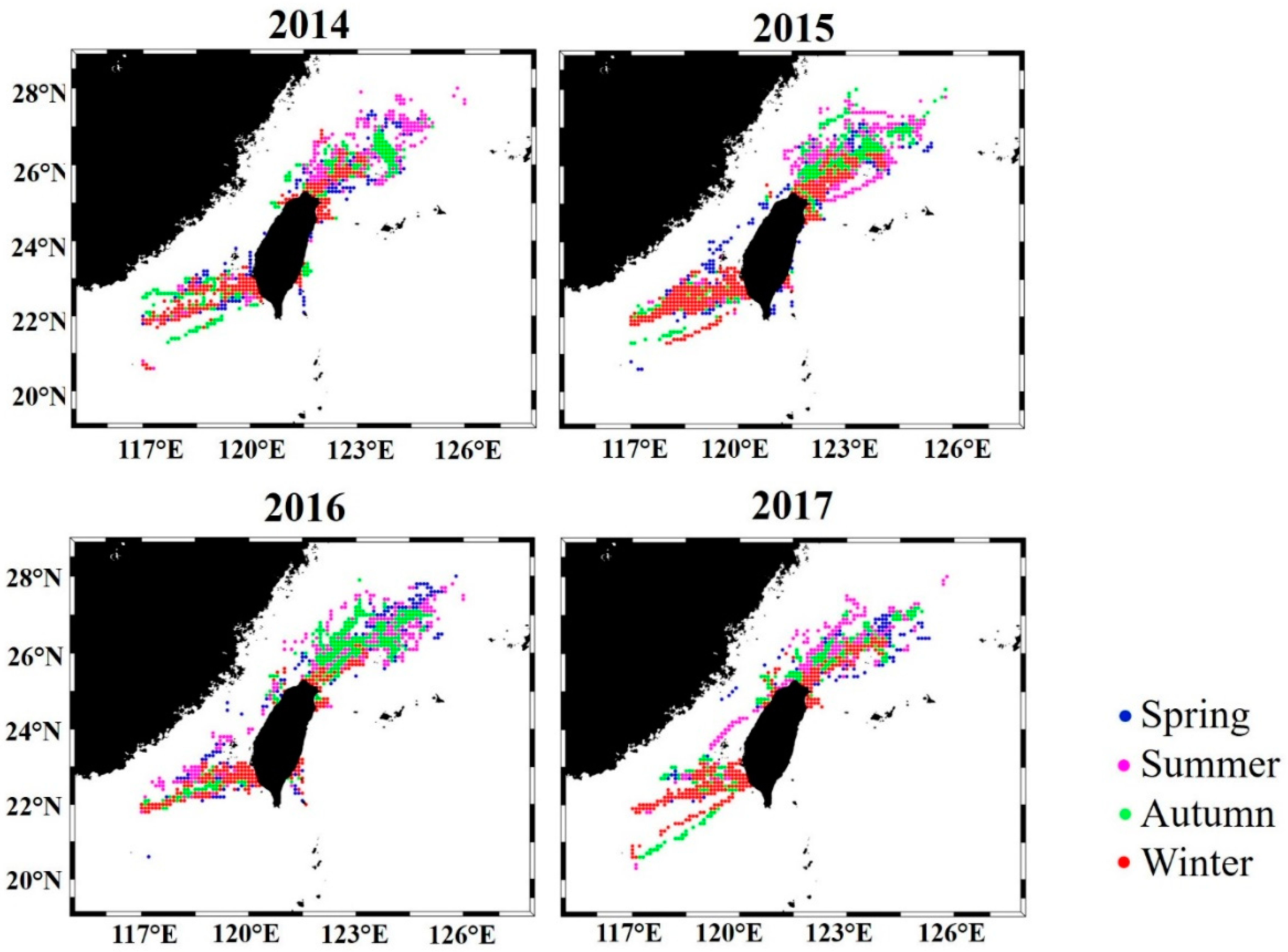
The spatial distribution pattern revealed that S. dumerili was extensively dispersed in the TS from the south to the north (20°N–29°N and 115°E–127°E), and angling gear was the most extensive fishing gear to harvest fish stocks (Figure 1). The seasonal fishing locations were widely distributed, and seasonal and annual fluctuations were identified based on the spatial distribution pattern of the seasonal fishing locations from 2014 to 2017 (Figure 2). The spatial distribution pattern exhibited a considerable seasonal change, as well as a change in fishing locations, probably influenced by S. dumerili capture trends. During spring, fishing locations were closer together, whereas, in summer and autumn, fishing locations were widely distributed northward, shifting southward during the winter.
The time-series trends of the latitudinal and longitudinal gravitational center of the catch rates (Figure 3a,b) and the monthly average environmental factors in the catch locations (Figure 3c–h) for S. dumerili revealed various trends in the TS. A strong association was detected between the environmental variables and S. dumerili catch rates. During the spring and summer, the longitudinal and latitudinal gravitational centers shifted northward (>24°N) and eastward (>122°E) as the SST increased (Figure 3a–c), whereas the SSS, SSH, Chl-a, and MLD decreased (Figure 3d–g). Regarding the latitudinal and longitudinal gravitational centers, the EKE exhibited a positive tendency, in the spring and summer, the current increases, whereas in the autumn and winter, it decreases (Figure 3h).

3.2. Environmental Effect on S. dumerili Catch Rates by Statistical Model

The two statistical models reveal that the predictor variables were chosen to represent the model selection resulting in the lowest residual factor, AIC values, and highest DE, indicating a better model fit. Because GAMs have the highest total DE and lower residual factor and AIC values than GLMs (Table 2 and Table 3), we employed the GAM fit to predict the catch rates of S. dumerili with environmental factors throughout the study area. The total DE using GAMs and adjusted r2 for S. dumerili was 47.3% (DE) and 0.47 (adjusted r2) in the 2014–2017 period (Table 3). When all the predictor variables were incorporated into the model, the stepwise approach used to identify the optimal predictor variables in combinations of the GAMs revealed the lowest AIC values and an increase in DE. All of the variables investigated in GAMs with S. dumerili in the TS were highly significant predictors (p < 0.001). The corrected AIC was employed as a measure of goodness-of-fit, with the optimal model having the lowest AIC value and highest DE. The latitude and longitude explained 15.1%, and 16.8%, respectively, of the DE (Table 3). SST exhibited the highest DE (22.9%), whereas MLD exhibited the lowest (2.46%; Table 3).
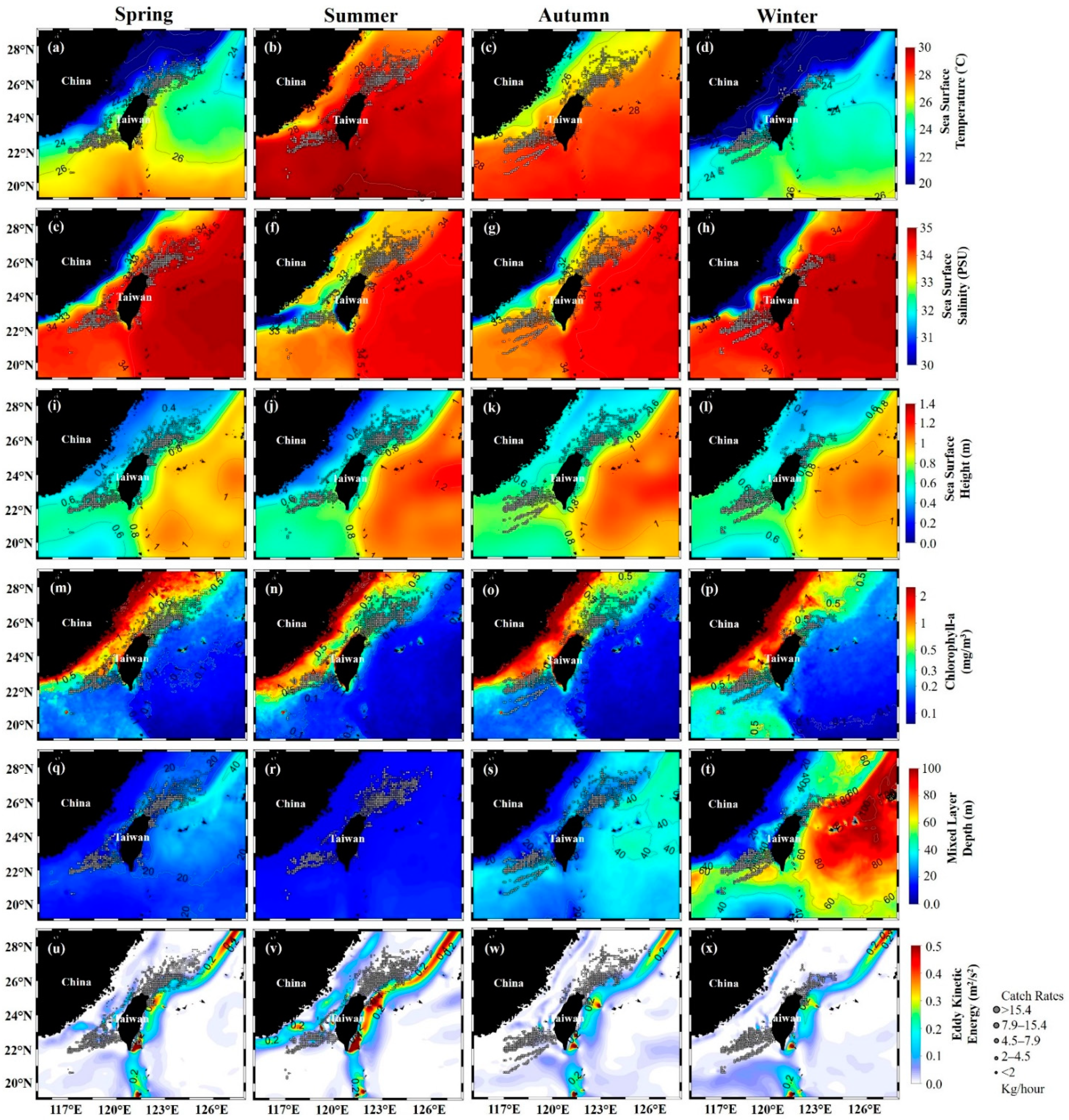
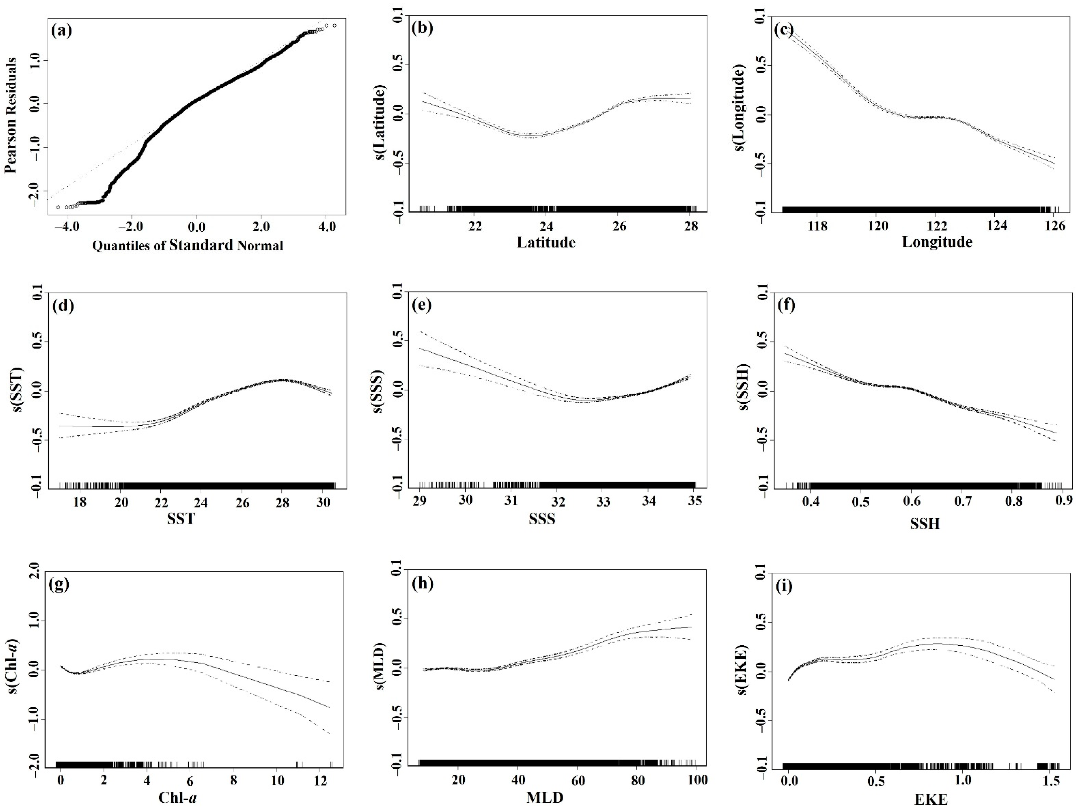
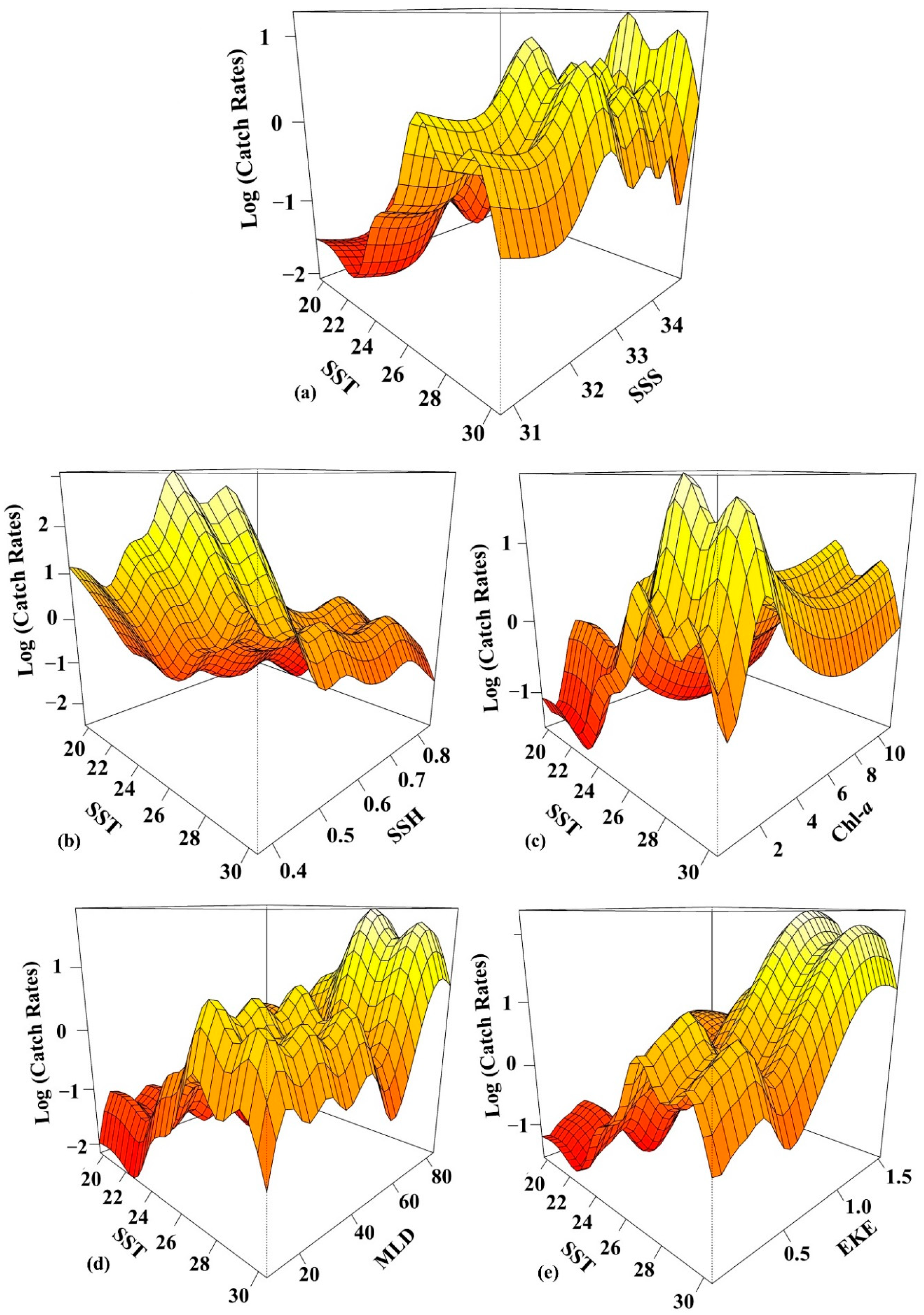
The seasonal spatial distribution pattern of the average observed catch rates subsequently overlaid with the selected environmental variables with the highest model explained the deviance percentages and revealed that the S. dumerili were predominantly abundant in the waters with SSTs of 22–28 °C, SSSs of 33–34.5 PSU, SSHs of 0.4–0.6 m, Chl-a of 0.5–1.5 mg/m3, MLDs of 10–50 m, and EKEs of 0.0–0.12 m2/s2 (Figure 4a–x). The satellite-observed oceanographic environmental variables had correlation coefficients ranging from r = −0.55 to 0.43; hence, all the variables were included in the model (Figure S1) in the Supplementary Material section. The RMSD value of GAM = (0.34 ± 0.01 SD); GLM = (0.39 ± 0.01 SD) (Figure 5). According to the GAM findings, S. dumerili catch rates increased from June to January, with a positive association with latitude > 25°N and longitude > 120°E (Figure 6a–c). In terms of the environmental variables, the S. dumerili catch rates exhibited a positive association with SSTs (26–28 °C), SSSs (33–34.5 PSU), and MLDs (>30 m), but a negative association was observed with SSHs > 0.6 m, Chl-a > 4 mg/m3, and EKEs > 0.4 m2/s2 (Figure 6d–i). The three-dimensional graph represents the interactions between the oceanic environmental factors and demonstrated that the variables were affecting the catch rates of S. dumerili in the TS (Figure 7a–e). The SST and SSS revealed that this interaction was the most significant contributor to S. dumerili catch rates in the model, with the preferred optimal ranges of SST (26–28 °C) and SSS (33–34.5 PSU) having the most influential on the model’s ability in terms of predicting potential fishing grounds (Figure 7a).

3.3. Predicted Spatial Distribution Pattern of the Greater Amberjack

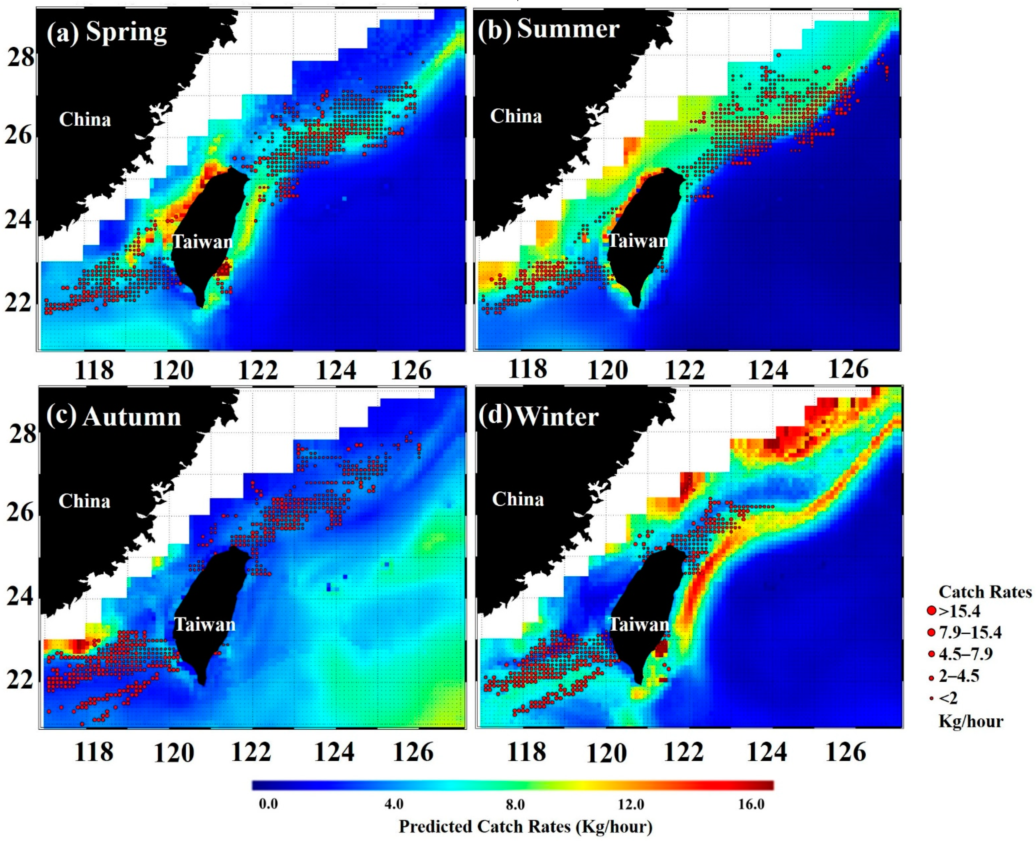
Figure 8 illustrates the seasonal predicted catch rates overlaid with the seasonal average observed catch rates for S. dumerili in the TS. Average seasonal observed catch rates were used to predict the main fishing locations with a high spatial resolution. Throughout the spring, relatively high S. dumerili catch rates were predicted in the northern region of the TS, whereas in summer, higher catch rates were predicted in the southwestern and throughout the northwestern region, including the prediction extending toward the waters of ECS (Figure 8a,b). The maps revealed during the summer, indicating the relatively highest predicted catch rates could explain the spatial distribution patterns of S. dumerili in the study area (Figure 8b). The catch rate for S. dumerili was predicted to be lower in autumn (Figure 8c). However, catch rates were predicted to increase again in winter in the southern region of the TS, and the relatively higher prediction in the northeastern part of Taiwan but did not match the observed catch rates (Figure 8d). As a result, the model is trustworthy, with good agreement with remotely sensed environmental factors and catch rates of S. dumerili fisheries in the waters of TS.
High S. dumerili catch rates were observed in the northern part of the TS, extending to 25°N–28°N and 122°E–126°E during the summer. Thus, the model-predicted catch rates were reliable, and they correlated well with the observed S. dumerili catch rates in the TS. Seasonal fluctuations in the predicted and RMSD values for S. dumerili were observed in 2019. In winter, spring and summer, the predicted values increased, whereas, in autumn, the predicted values decreased. Seasonally, the RMSD value was calculated as 0.35–0.48 (Table 4).

4. Discussion

4.1. Distribution of Greater Amberjack in the Taiwan Strait

Identifying the spatiotemporal distribution patterns of target species in relation to observed catch rates and preferred environmental factors is essential for fishery conservation, management, and spatial planning. The present study demonstrated a comprehensive framework for spatiotemporal distribution patterns of S. dumerili in the TS; we used GAM as a tool for the evaluation the model’s fitting performance, species distribution pattern, predictive capacity, and model stability. Our findings highlighted a significant relationship between observed S. dumerili catch rates and oceanic environments, with the species distributed from the southern part to the northern part across the TS. Hasegawa et al. [13,16] reported that S. dumerili is a common species around the Taiwan Bank and distributed between the southern and northern parts of the TS. This study revealed that the predicted catch rates of S. dumerili distribution were highest in the northern region of TS during spring; the catch rates were high, and the area with high catch rates was widely distributed southward to northward during summer and comparatively, it predicted lower rates in autumn and increased predicted catch rates again in the southern part of TS, and relatively higher prediction in the northeastern part Taiwan but not matching the observed catch rates in the winter. Many marine fish species have distinct spatial distribution patterns, with habitat preferences based on physiological requirements or oceanographic environmental tolerance [32]. In particular, our time-series investigations on the spatiotemporal distribution patterns of the commercially valuable S. dumerili reveal that environmental factors influence the species’ habitat formation. These findings will also be more helpful in defining a common harvest strategy plan, which is critical for future stock utilization and sustainable fishing.
S. dumerili spawn along the continental shelf’s edge in the northern waters of Taiwan in the southern ECS mainly from February to April, according to an investigation of the early larvae distribution [13] and the seasonal gonadal development of adults [44]. Our findings noted that in the spring, the spatiotemporal distribution pattern of S. dumerili is higher in the southern part of the ECS, which has favorable oceanographic characteristics because of the Kuroshio Branch Current and Kuroshio Current [45]. Tone et al. [46] reported that the S. dumerili spawning ground in February and March was located in the ECS. Our model predicted that in spring, catch rates would be high in the northern part of the TS, whereas in summer, these rates would increase further and the area with a high catch rate would extend toward the ECS. Research has identified marine species spawning grounds in the inshore seas of northern Taiwan in the ECS, where the warm Kuroshio transported them to the front feeding areas over the continental shelf [36]. In the autumn, catch rates were predicted to be lower in our investigation, possibly due to the spatial predictions of the GAM models revealing that EKE was the lowest DE. Although, Teng et al. [30] mentioned that the movement of the Kuroshio Branch Current in the coastal waters of TS during autumn might substantially impact the habitats of various marine species. However, the catch rates were predicted to be higher and the majority of fishing locations during this period were in the southern part of TS, and relatively higher predictions were in the northeastern part of Taiwan but did not match the observed catch rates (Figure 8d). Because the spatial prediction follows the upstream flow of strong warm water Kuroshio Current path, which passes through the northeastern part of Taiwan, potentially, SST is the important factor explaining the highest deviance in our model. S. dumerili prefers a low water current (Figure 4) which may be the reason why observed catch rates did not match. Many studies have reported that the Kuroshio Current, which flows close to the coastal area near the northeastern part of Taiwan [47,48,49].
The Kuroshio Current is strongly associated with the transportation and distribution pattern of S. dumerili in the surrounding waters of Taiwan [13]. In addition, Tone et al. [46] reported that in winter, the strong northeasterly wind blows continuously above the continental shelf of the ECS, cooling the water and enabling the S. dumerili to satisfy their energy needs for gamete growth and subsequent spawning activities. In Figure 8, we removed the spatial prediction of coastal waters of the mainland China region, because of the high discharge of nutrient-rich sediments water from the Yangtze River discharge through the Yellow Sea and the East Sea over the ECS, which leads to high plankton bloom [50,51], so the S. dumerili predominantly prefer to live over the SST frontal area. According to studies, they have a key function in the SST frontal region for providing a suitable habitat area with favorable oceanographic conditions for fish species in the northern and southern parts of the TS [52,53,54,55]. The SST frontal areas are an important characteristic region, especially for large pelagic fish species like tunas, to enhance their foraging success and advantages of the physiological process [56].
Fish distributions are influenced by the energy requirements of feeding, but including these types of ecological features in spatiotemporal modeling is challenging. However, SST is one of the important variables directly associated with species and their prey’s physiological requirements [25]. The physiological constraints of species are a key driver of their spatiotemporal distributions, and temperature preferences for tuna [29,31,57,58] and marlin [59] have been established using spatiotemporal distribution models. S. dumerili distribution was widely distributed and high catch rates were predicted in the northern region of TS in summer; however, the high catch rate prediction extended toward the ECS (Figure 2 and Figure 8b). This might be because of the availability of food and the preferred habitat-related oceanographic conditions conducive to development and survival. The mesozooplankton community in the Kuroshio region has comparable standing stock and productivity to those on the ECS shelf, indicating that sufficient food was available for the S. dumerili in this region and the warm water transported by the Kuroshio Current was optimal [46,60]. The distribution, migration, and availability of fish shoals are strongly linked to the oceanic fronts [52,61].
The nutrient-rich cold water of the China Coastal Current intrusion in the northern region of the TS may alter the movement of S. dumerili to migrate to the southwestern part of the TS during the winter (Figure 8d). Therefore, our findings support those of Tzeng et al. [62], who reported that the southward intruding China Coastal Current flows from the northwestern tip of the TS in winter. Consequently, the spatiotemporal pattern results of the current study reflected the general distribution patterns of S. dumerili in Taiwanese waters. Therefore, the oceanographic environmental conditions of the preferred habitat for the S. dumerili in the TS were accurately predicted by the GAM in this study.

4.2. Environmental Factors Affecting the Greater Amberjack

Currently, S. dumerili is considered to be overfished globally because of increased fishing effort and landings [63]. However, in the TS, its status is unclear, and no management or conservation plans exist for the species. Therefore, the species’ response to environmental factors and habitat preferences should be explored to ensure appropriate fisheries management approaches are implemented to maintain fishing at a sustainable level. Our findings demonstrated that the catch rates were linked to relevant environmental characteristics in the TS depending on the season and habitat and in accordance with the S. dumerili temporal and spatial distribution pattern. SST and SSS were the variables with the highest DE in the GAM for S. dumerili in the TS. SST was a highly significant factor for predicting suitable environmental conditions for the species. Although the conditions varied over time and space, they are crucial for understanding the habitat selection of S. dumerili in the eastern waters of Taiwan [46]. SST and SSS both have a substantial impact on the spatial and temporal distributions of marine fish [10,64]. Generally, the warm water SCS Current and Kuroshio Branch Current are dominant in summer, transporting high-saline warm water with fewer nutrients, whereas the China Coastal Current, carried by strong northeasterly winds, transports low-saline nutrient-enriched cold water southward through the western region of the TS [65]. The complex structures in the exchange of the water column mixing and the numerous current systems in the TS influence the variations in the key oceanographic environmental factors, such as the SST and SSS, which affect the temporal and spatial distribution of target species. According to studies, environmental factors such as the SST, EKE, sea-level anomaly, and dissolved oxygen have been found to influence the Seriola species diversity and distribution patterns over time and space [24,25,26].
In the present study, using multiple environmental variables to predict S. dumerili oceanographic habitats at monthly and seasonal time series revealed significant shifts in the temporal and spatial distribution patterns of preferred habitats from south to north of the TS over the study period. The spatial and temporal fluctuation of fish assemblages is significantly linked to the oceanic environment; thus, satellite remote sensing can be employed to provide clear data and accurately predict the abundance and distribution of potential fishing grounds for pelagic species [10,25]. SSH is another major environmental factor that significantly influences the distribution pattern as well as the catch rates and habitat of S. dumerili in the TS, and our findings revealed that the preferred SSH range is 0.4–0.6 m (Figure 4). Similarly, SSH is linked to foraging and can be used to identify the ecological zones in the ocean with similar physical and biological forces that affect sea productivity and pelagic species occurrence [11,39,66,67]. Throughout the year, the subsurface water upwelling in the Kuroshio region at the Taiwanese continental shelf supplies enriching nutrients to the water [36].
The Chl-a concentration is a key environmental factor for upwelling and primary productivity in the ocean, which is a phytoplankton-related parameter that can be used to predict S. dumerili spatial and temporal distribution. We observed high S. dumerili catch rates at Chl-a concentrations of 0.5–1.5 mg/m3 in the TS (Figure 4). S. dumerili is not a direct phytoplankton consumer, but phytoplankton distribution has a considerable impact on the trophic interactions involving prey–predator connections in the food chain [68]. Lee et al. [31] reported that the spatiotemporal distribution pattern and abundance variability of albacore tuna is strongly linked with the Chl-a distribution in the North Pacific Ocean, despite the fact that there is no direct connection in the food web between albacore tuna and phytoplankton. In general, grazers such as zooplankton play an important role in the food chain and are strongly associated with phytoplankton distribution [68]. Zooplankton populations are a primary food source for both young and adult S. dumerili, as well as small pelagic fish. These indirect relationships between S. dumerili and phytoplankton populations are used to estimate the abundance and availability of the target species based on various oceanographic features, such as Chl-a concentration.
Bathymetric surveys conducted in the coastal waters of Taiwan have revealed that the average water depth in the western coastal areas (<50 m) is lower than that in the eastern coastal areas (>2000 m) [69]. Water depth is a key oceanographic feature that influences the shape and structure of marine species communities. While the model revealed that the SST and SSS had the highest DE, other environmental factors play a role in determining the varying amounts of DE in the model contribution, most likely due to changes in the oceanographic features related to S. dumerili habitats. We observed the highest catch rates for S. dumerili at an MLD of between 10 and 50 m (Figure 4). Similarly, in March, S. dumerili was found in the Gulf of Mexico’s central-western and northern shores at shallower depths ranging from 11 to 50 m [70], when the water in nutrient sediment traps was well mixed throughout the seasonal flux [71]. By combining these findings, we propose that the topographic features related to foraging are those that attract planktonic assemblages and that oceanographic characteristics such as the Kuroshio Warm Current have influenced the spatial and temporal distribution pattern of S. dumerili in the TS.
Several currents, such as the SCS Surface Current, Kuroshio Current, Kuroshio Branch Current, and China Coastal Current have a substantial influence on the marine organisms in the waters surrounding Taiwan [72,73]. Furthermore, the varying topography has a large influence on the fluctuation of these currents; consequently, the currents alter the oceanographic environmental conditions in the waters around Taiwan throughout the year [74,75]. These variable conditions are responsible for the diverse spatiotemporal distribution pattern for S. dumerili in the TS. Research has demonstrated that low EKE values are associated with kingfish (S. lalandi) habitat characteristics, abundant in Australian waters, with EKE values of 0.11 [26] and 0.16 m2/s2 [25]. Despite our findings, we noted that S. dumerili was predominantly abundant in the waters of the TS with EKE values of 0.0–0.12 m2/s2 (Figure 4). Although our research only focused on the S. dumerili catch rates in the seasonal distribution patterns with environmental changes, we believe that climate-related changes may have an impact on S. dumerili catch rates, which should be investigated further. However, the current study had important limitations, such as the SST frontal area, which is associated with the habitat of large pelagic species, and we only use the GLM and GAM models to analyze the spatiotemporal distribution pattern of S. dumerili. Therefore, future research should consider the SST frontal data, and also include other habitat models such as the Geometric Mean Model [7], Arithmetic Mean Model [10], and Maximum Entropy Model [30,76], which one can apply and compare which is better for S. dumerili habitats.

5. Conclusions

In this study, we used satellite-derived remote sensing oceanographic environmental factors and daily high-resolution fisheries data to estimate the spatiotemporal distribution patterns of S. dumerili in the TS. SST and SSS were the key environmental factors influencing the spatial pattern and might be linked to seasonal variations in the TS; these two factors were associated with higher catch rates. Other environmental variables also played a key role in the distribution of the targeted species. Positive associations were identified between SSTs (26–28 °C) and SSSs (33–34.5 PSU) that had high S. dumerili catch rates. The model predicted that high catch rates would be observed primarily in the northwestern region of the TS in summer. Our reliable and valid data for predicting potential fishing locations can help fishers employ precision fishing through the targeted exploitation of identified species. Fishers will be able to increase their catch in less time at a sustainable level, reducing their carbon footprint and bycatch, which has both economic and environmental benefits. The results of the best GAMs prediction performance of the distribution patterns of S. dumerili habitats are in good agreement with the predicted map and observation data. Furthermore, when habitat suitability models are used to predict fishing grounds and habitat preferences, fishing can be conducted more efficiently. This primary research goal may facilitate a better understanding of S. dumerili catch rates with environmental variation in the TS, as well as future conservation strategies and fisheries management priorities.

Supplementary Materials

The following supporting information can be downloaded at: https://www.mdpi.com/article/10.3390/rs14122932/s1, Figure S1: Multiple correlation coefficients for the relationship between greater amberjack oceanographic habitat preferences on the basis of satellite-observed environmental variables; all the environmental factors with correlation coefficients ranging from r = −0.55 to 0.43.

Author Contributions

Conceptualization, M.M. and M.-A.L.; methodology, M.M. and M.N.; software, M.M., M.N. and J.-H.W.; validation, A.H.V., J.H., Y.-C.W. and M.-A.L.; formal analysis, K.-W.L., A.H.V., J.H. and M.-A.L.; investigation, Y.-C.W., K.-W.L. and M.-A.L.; resources, Y.-C.W. and M.-A.L.; data curation, M.M. and M.-A.L.; writing—original draft preparation, M.M.; writing—review and editing, M.M., M.N., A.H.V., J.H., K.-W.L. and M.-A.L.; visualization, Y.-C.W.; supervision, M.-A.L. All authors have read and agreed to the published version of the manuscript.

Funding

This research received no external funding.

Acknowledgments

This research was supported in part by the Ministry of Science and Technology (MOST 108-2611-M-019-008, MOST 109-2611-M-019-006, and MOST 110-2611-M-019-010), Taiwan. We also thank the Fishery Agency of the Council of Agriculture, Executive Yuan, R.O.C. for providing information and assistance for this research.

Conflicts of Interest

The authors declare no conflict of interest.

References

  1. Saraux, C.; Fromentin, J.M.; Bigot, J.L.; Bourdeix, J.H.; Morfin, M.; Roos, D.; Van Beveren, E.; Bez, N. Spatial structure and distribution of small pelagic fish in the northwestern Mediterranean Sea. PLoS ONE 2014, 9, 111211. [Google Scholar]
  2. Garrison, L.P.; Michaels, W.; Link, J.S.; Fogarty, M.J. Spatial distribution and overlap between ichthyoplankton and pelagic fish and squids on the southern flank of Georges Bank. Fish. Oceanogr. 2002, 11, 267–285. [Google Scholar] [CrossRef]
  3. Azevedo, M.; Silva, C. A framework to investigate fishery dynamics and species size and age spatio-temporal distribution patterns based on daily resolution data: A case study using Northeast Atlantic horse mackerel. ICES J. Mar. Sci. 2020, 77, 2933–2944. [Google Scholar] [CrossRef]
  4. Ward, E.J.; Jannot, J.E.; Lee, Y.W.; Ono, K.; Shelton, A.O.; Thorson, J.T. Using spatiotemporal species distribution models to identify temporally evolving hotspots of species co-occurrence. Ecol. Appl. 2015, 25, 2198–2209. [Google Scholar] [CrossRef]
  5. Kai, M.; Thorson, J.T.; Piner, K.R.; Maunder, M.N. Predicting the spatio-temporal distributions of pelagic sharks in the western and central North Pacific. Fish. Oceanogr. 2017, 26, 569–582. [Google Scholar] [CrossRef]
  6. Lee, M.A.; Vayghan, A.H.; Liu, D.C.; Yang, W.C. Potential and prospective seasonal distribution of hotspot habitat of albacore tuna (Thunnus alalunga) in the South Indian Ocean using the satellite data. In Proceedings of the 2017 IEEE International Geoscience and Remote Sensing Symposium (IGARSS), Fort Worth, TX, USA, 23–28 July 2017; pp. 5747–5750. [Google Scholar]
  7. Vayghan, A.H.; Lee, M.A.; Weng, J.S.; Mondal, S.; Lin, C.T.; Wang, Y.C. Multisatellite-based feeding habitat suitability modeling of albacore tuna in the Southern Atlantic Ocean. Remote Sens. 2020, 12, 2515. [Google Scholar] [CrossRef]
  8. Mansor, S.; Tan, C.K.; Ibrahim, H.M.; Shariff, A.R.M. Satellite fish forecasting in south China sea. In Proceedings of the 22nd Asian Conference on Remote Sensing, Singapore, 5–9 November 2001; Volume 5. No. 9. [Google Scholar]
  9. Zhang, X.; Saitoh, S.I.; Hirawake, T. Predicting potential fishing zones of japanese common squid (Todarodes Pacificus) using remotely sensed images in coastal waters of south-western Hokkaido, Japan. Int. J. Remote Sens. 2017, 38, 6129–6146. [Google Scholar] [CrossRef]
  10. Lee, D.; Son, S.; Kim, W.; Park, J.M.; Joo, H.; Lee, S.H. Spatio-temporal variability of the habitat suitability index for Chub Mackerel (Scomber japonicus) in the East/Japan sea and the South sea of South Korea. Remote Sens. 2018, 10, 938. [Google Scholar] [CrossRef] [Green Version]
  11. Abdul Azeez, P.; Raman, M.; Rohit, P.; Shenoy, L.; Jaiswar, A.K.; Mohammed Koya, K.; Damodaran, D. Predicting potential fishing grounds of ribbonfish (Trichiurus lepturus) in the north-eastern Arabian Sea, using remote sensing data. Int. J. Remote Sens. 2021, 42, 322–342. [Google Scholar] [CrossRef]
  12. Taki, Y.; Kohno, H.; Sakamaot, K.; Hosoya, K. Illustrated Fishes in Colour Revised Edition; Hokuryukan Co., Ltd.: Tokyo, Japan, 2005. (In Japanese) [Google Scholar]
  13. Hasegawa, T.; Lu, C.P.; Hsiao, S.T.; Uchino, T.; Yeh, H.M.; Chiang, W.C.; Chen, J.R.; Sassa, C.; Komeyama, K.; Kawabe, R.; et al. Distribution and genetic variability of young-of-the-year greater amberjack (Seriola dumerili) in the East China Sea. Environ. Biol. Fishes 2020, 103, 833–846. [Google Scholar] [CrossRef]
  14. Thompson, B.A.; Beasley, M.; Wilson, C.A. Age distribution and growth of greater amberjack, Seriola dumerili, from the north-central Gulf of Mexico. Fish. Bull. 1999, 97, 362–371. [Google Scholar]
  15. Wells, R.J.; Rooker, J.R. Distribution, age, and growth of young-of-the year greater amberjack (Seriola dumerili) associated with pelagic Sargassum. Fish. Bull. 2004, 102, 545–554. [Google Scholar]
  16. Hasegawa, T.; Yeh, H.M.; Chen, J.R.; Kuo, C.L.; Kawabe, R.; Sakakura, Y. Collection and aging of greater amberjack Seriola dumerili larvae and juveniles around the Penghu Islands, Taiwan. Ichthyol. Res. 2017, 64, 145–150. [Google Scholar] [CrossRef] [Green Version]
  17. Sassa, C.; Tsukamoto, Y.; Nishiuchi, K.; Konishi, Y. Spawning ground and larval transport processes of jack mackerel Trachurus japonicus in the shelf-break region of the southern East China Sea. Cont. Shelf Res. 2008, 28, 2574–2583. [Google Scholar] [CrossRef]
  18. Sassa, C.; Tsukamoto, Y. Distribution and growth of Scomber japonicus and S. australasicus larvae in the southern East China Sea in response to oceanographic conditions. Mar. Ecol. Prog. Ser. 2010, 419, 185–199. [Google Scholar] [CrossRef] [Green Version]
  19. Fisher, W.; Bianchi, G.; Scott, W.B. FAO Species Identification Guides for Fishery Purposes; Volume 3, Eastern Central Atlantic, Fishing Area 34 and Part of 47; Food and Agriculture Organization: Ottawa, ON, Canada, 1981. [Google Scholar]
  20. Huh, C.A.; Chen, W.; Hsu, F.H.; Su, C.C.; Chiu, J.K.; Lin, S.; Liu, C.S.; Huang, B.J. Modern (<100 years) sedimentation in the Taiwan Strait: Rates and source-to-sink pathways elucidated from radionuclides and particle size distribution. Cont. Shelf Res. 2011, 31, 47–63. [Google Scholar] [CrossRef]
  21. Naimullah, M.; Lan, K.W.; Liao, C.H.; Hsiao, P.Y.; Liang, Y.R.; Chiu, T.C. Association of environmental factors in the Taiwan strait with distributions and habitat characteristics of three swimming crabs. Remote Sens. 2020, 12, 2231. [Google Scholar] [CrossRef]
  22. Zainuddin, M.; Saitoh, S.I.; Saitoh, K. Detection of potential fishing ground for albacore tuna using synoptic measurements of ocean color and thermal remote sensing in the northwestern North Pacific. Geophys. Res. Lett. 2004, 31. [Google Scholar] [CrossRef]
  23. Chen, I.C.; Lee, P.F.; Tzeng, W.N. Distribution of albacore (Thunnus alalunga) in the Indian Ocean and its relation to environmental factors. Fish. Oceanogr. 2005, 14, 71–80. [Google Scholar] [CrossRef]
  24. Tian, Y.; Kidokoro, H.; Watanabe, T.; Igeta, Y.; Sakaji, H.; Ino, S. Response of yellowtail, Seriola quinqueradiata, a key large predatory fish in the Japan Sea, to sea water temperature over the last century and potential effects of global warming. J. Mar. Syst. 2012, 91, 1–10. [Google Scholar] [CrossRef]
  25. Brodie, S.; Hobday, A.J.; Smith, J.A.; Everett, J.D.; Taylor, M.D.; Gray, C.A.; Suthers, I.M. Modelling the oceanic habitats of two pelagic species using recreational fisheries data. Fish. Oceanogr. 2015, 24, 463–477. [Google Scholar] [CrossRef]
  26. Champion, C.; Hobday, A.J.; Zhang, X.; Pecl, G.T.; Tracey, S.R. Changing windows of opportunity: Past and future climate-driven shifts in temporal persistence of kingfish (Seriola lalandi) oceanographic habitat within south-eastern Australian bioregions. Mar. Freshw. Res. 2018, 70, 33–42. [Google Scholar] [CrossRef]
  27. Furukawa, S.; Kozuka, A.; Tsuji, T.; Kubota, H. Horizontal and vertical movement of yellowtails Seriola quinqueradiata during summer to early winter recorded by archival tags in the northeastern Japan Sea. Mar. Ecol. Prog. Ser. 2020, 636, 139–156. [Google Scholar] [CrossRef]
  28. Sassa, C.; Takahashi, M.; Konishi, Y.; Yoshimasa, A.; Tsukamoto, Y. The rapid expansion of yellowtail (Seriola quinqueradiata) spawning ground in the East China Sea is linked to increasing recruitment and spawning stock biomass. ICES J. Mar. Sci. 2020, 77, 581–592. [Google Scholar] [CrossRef]
  29. Mondal, S.; Vayghan, A.H.; Lee, M.A.; Wang, Y.C.; Semedi, B. Habitat suitability modeling for the feeding ground of immature albacore in the Southern Indian Ocean using satellite-derived sea surface temperature and chlorophyll data. Remote Sens. 2021, 13, 2669. [Google Scholar] [CrossRef]
  30. Teng, S.Y.; Su, N.J.; Lee, M.A.; Lan, K.W.; Chang, Y.; Weng, J.S.; Wang, Y.C.; Sihombing, R.I.; Vayghan, A.H. Modeling the habitat distribution of Acanthopagrus schlegelii in the coastal waters of the Eastern Taiwan strait using MAXENT with fishery and remote sensing data. J. Mar. Sci. Eng. 2021, 9, 1442. [Google Scholar] [CrossRef]
  31. Lee, M.A.; Weng, J.S.; Lan, K.W.; Vayghan, A.H.; Wang, Y.C.; Chan, J.W. Empirical habitat suitability model for immature albacore tuna in the North Pacific Ocean obtained using multisatellite remote sensing data. Int. J. Remote Sens. 2020, 41, 5819–5837. [Google Scholar] [CrossRef]
  32. Guisan, A.; Zimmermann, N.E. Predictive habitat distribution models in ecology. Ecol. Modell. 2000, 135, 147–186. [Google Scholar] [CrossRef]
  33. Wang, L.; Kerr, L.A.; Record, N.R.; Bridger, E.; Tupper, B.; Mills, K.E.; Armstrong, E.M.; Pershing, A.J. Modeling marine pelagic fish species spatiotemporal distributions utilizing a maximum entropy approach. Fish. Oceanogr. 2018, 27, 571–586. [Google Scholar] [CrossRef]
  34. Elith, J.; Leathwick, J.R. Species distribution models: Ecological explanation and prediction across space and time. Annu. Rev. Ecol. Evol. Syst. 2009, 40, 677–697. [Google Scholar] [CrossRef]
  35. Solanki, H.U.; Bhatpuria, D.; Chauhan, P. Applications of generalized additive model (GAM) to satellite-derived variables and fishery data for prediction of fishery resources distributions in the Arabian Sea. Geocarto Int. 2017, 32, 30–43. [Google Scholar] [CrossRef]
  36. Liao, C.H.; Lan, K.W.; Ho, H.Y.; Wang, K.Y.; Wu, Y.L. Variation in the catch rate and distribution of swordtip squid Uroteuthis edulis associated with factors of the oceanic environment in the Southern East China Sea. Mar. Coast. Fish. 2018, 10, 452–464. [Google Scholar] [CrossRef] [Green Version]
  37. Hastie, T.; Tibshirani, R. Generalized additive models. Stat. Sci. 1986, 1, 297–310. [Google Scholar] [CrossRef]
  38. Zainuddin, M.; Saitoh, K.; Saitoh, S.I. Albacore (Thunnus alalunga) fishing ground in relation to oceanographic conditions in the western North Pacific Ocean using remotely sensed satellite data. Fish. Oceanogr. 2008, 17, 61–73. [Google Scholar] [CrossRef] [Green Version]
  39. Lan, K.W.; Shimada, T.; Lee, M.A.; Su, N.J.; Chang, Y. Using remote-sensing environmental and fishery data to map potential yellowfin tuna habitats in the tropical Pacific Ocean. Remote Sens. 2017, 9, 444. [Google Scholar] [CrossRef] [Green Version]
  40. QGIS Development Team. QGIS 3.6 Noosa. Available online: https://qgis.org/en/site (accessed on 30 September 2019).
  41. Lan, K.W.; Evans, K.; Lee, M.A. Effects of climate variability on the distribution and fishing conditions of yellowfin tuna (Thunnus albacares) in the western Indian Ocean. Clim. Chang. 2013, 119, 63–77. [Google Scholar] [CrossRef] [Green Version]
  42. Chai, T.; Draxler, R.R. Root mean square error (RMSE) or mean absolute error (MAE)?—Arguments against avoiding RMSE in the literature. Geosci. Model Dev. 2014, 7, 1247–1250. [Google Scholar] [CrossRef] [Green Version]
  43. R Core Team. R: A Language and Environment for Statistical Computing; R Foundation for Statistical Computing: Vienna, Austria, 2021. [Google Scholar]
  44. Hsiao, S.T.; Li, C.H.; Yeh, H.M. Seasonal changes in the gonadosomatic index of the greater amberjack in Taiwanese waters. 2016; Unpublished raw data. [Google Scholar]
  45. Yue, J.; Noman, M.A.; Sun, J. Kuroshio intrusion drives the Trichodesmium assemblage and shapes the phytoplankton community during spring in the East China Sea. J. Oceanol. Limnol. 2021, 39, 536–549. [Google Scholar] [CrossRef]
  46. Tone, K.; Nakamura, Y.; Chiang, W.C.; Yeh, H.M.; Hsiao, S.T.; Li, C.H.; Komeyama, K.; Tomisaki, M.; Hasegawa, T.; Sakamoto, T.; et al. Migration and spawning behavior of the greater amberjack Seriola dumerili in eastern Taiwan. Fish. Oceanogr. 2022, 31, 1–18. [Google Scholar] [CrossRef]
  47. Yin, W.; Huang, D. Short-term variations in the surface upwelling off northeastern Taiwan observed via satellite data. J. Geophys. Res. Oceans 2019, 124, 939–954. [Google Scholar] [CrossRef]
  48. Zhuang, Z.; Zheng, Q.; Zhang, X.; Yang, G.; Zhao, X.; Cao, L.; Zhang, T.; Yuan, Y. Variability of Kuroshio surface axis northeast of Taiwan island derived from satellite altimeter data. Remote Sens. 2020, 12, 1059. [Google Scholar] [CrossRef] [Green Version]
  49. Kang, J.; Na, H. Long-term variability of the Kuroshio shelf intrusion and its relationship to upper-ocean current and temperature variability in the East China Sea. Front. Mar. Sci. 2022, 9, 812911. [Google Scholar] [CrossRef]
  50. Chen, L.; Dong, C.; Wang, G. GOCI-observed chlorophyll belts associated with sea-surface fronts in the East China Sea. IEEE Geosci. Remote. Sens. Lett. 2019, 17, 1299–1302. [Google Scholar] [CrossRef]
  51. Park, M.S.; Lee, S.; Ahn, J.H.; Lee, S.J.; Choi, J.K.; Ryu, J.H. Decadal measurements of the first Geostationary Ocean Color Satellite (GOCI) compared with MODIS and VIIRS data. Remote Sens. 2021, 14, 72. [Google Scholar] [CrossRef]
  52. Lan, K.W.; Kawamura, H.; Lee, M.A.; Chang, Y.; Chan, J.W.; Liao, C.H. Summertime sea surface temperature fronts associated with upwelling around the Taiwan Bank. Cont. Shelf Res. 2009, 29, 903–910. [Google Scholar] [CrossRef]
  53. Chang, Y.; Shimada, T.; Lee, M.A.; Lu, H.J.; Sakaida, F.; Kawamura, H. Wintertime sea surface temperature fronts in the Taiwan Strait. Geophys. Res. Lett. 2006, 33. [Google Scholar] [CrossRef]
  54. Chang, Y.; Lee, M.A.; Shimada, T.; Sakaida, F.; Kawamura, H.; Chan, J.W.; Lu, H.J. Wintertime high-resolution features of sea surface temperature and chlorophyll-a fields associated with oceanic fronts in the southern East China Sea. Int. J. Remote Sens. 2008, 29, 6249–6261. [Google Scholar] [CrossRef]
  55. Lee, M.A.; Chang, Y.; Shimada, T. Seasonal evolution of fine-scale sea surface temperature fronts in the East China Sea. Deep Sea Res. Part II Top. Stud. Oceanogr. 2015, 119, 20–29. [Google Scholar] [CrossRef]
  56. Snyder, S.; Franks, P.J.; Talley, L.D.; Xu, Y.; Kohin, S. Crossing the line: Tunas actively exploit submesoscale fronts to enhance foraging success. Limnol. Oceanogr. Lett. 2017, 2, 187–194. [Google Scholar] [CrossRef]
  57. Vayghan, A.H.; Lee, M.A. Hotspot habitat modeling of skipjack tuna (Katsuwonus pelamis) in the Indian Ocean by using multisatellite remote sensing. Turk. J. Fish. Aquat. Sci. 2022, 22, TRJFAS19107. [Google Scholar] [CrossRef]
  58. Arrizabalaga, H.; Dufour, F.; Kell, L.; Merino, G.; Ibaibarriaga, L.; Chust, G.; Irigoien, X.; Santiago, J.; Murua, H.; Fraile, I.; et al. Global habitat preferences of commercially valuable tuna. Deep-Sea Res. II Top. Stud. Oceanogr. 2015, 113, 102–112. [Google Scholar] [CrossRef] [Green Version]
  59. Lien, Y.H.; Su, N.J.; Sun, C.L.; Punt, A.; Yeh, S.Z.; DiNardo, G. Spatial and environmental determinants of the distribution of Striped Marlin (Kajikia audax) in the western and central North Pacific Ocean. Environ. Biol. Fishes 2014, 97, 267–276. [Google Scholar] [CrossRef]
  60. Hirata, Y.; Hamasaki, K.; Imai, A.; Teruya, K.; Iwasaki, T.; Hamada, K.; Mushiake, K. Effects of different photoperiods and water temperatures on survival, growth, feeding and initial swim bladder inflation of greater amberjack Seriola dumerili larvae. Nippon Suisan Gakkaishi 2009, 75, 995–1003, (In Japanese with English abstract). [Google Scholar] [CrossRef] [Green Version]
  61. Zainuddin, M.; Kiyofuji, H.; Saitoh, K.; Saitoh, S.I. Using multi-sensor satellite remote sensing and catch data to detect ocean hot spots for albacore (Thunnus alalunga) in the northwestern North Pacific. Deesp-Sea Res. II Top. Stud. Oceanogr. 2006, 53, 419–431. [Google Scholar] [CrossRef]
  62. Tzeng, M.T.; Lan, K.W.; Chan, J.W. Interannual variability of wintertime sea surface temperatures in the eastern Taiwan Strait. J. Mar. Sci. Tech-Taiw. 2012, 20, 14. [Google Scholar]
  63. Turner, S.C.; Cummings, N.J.; Porch, C.P. Stock assessments of Gulf of Mexico greater amberjack using data through 1998. In Southeast Data, Assessment and Review; S9RD06; SEDAR: North Charleston, SC, USA, 2000. [Google Scholar]
  64. Castillo, J.; Barbieri, M.A.; Gonzalez, A. Relationships between sea surface temperature, salinity, and pelagic fish distribution off northern Chile. ICES J. Mar. Sci. 1996, 53, 139–146. [Google Scholar] [CrossRef]
  65. Jan, S.; Tseng, Y.H.; Dietrich, D.E. Sources of water in the Taiwan Strait. J. Oceanogr. 2010, 66, 211–221. [Google Scholar] [CrossRef]
  66. Chen, X.; Li, G.; Feng, B.; Tian, S. Habitat suitability index of chub mackerel (Scomber japonicus) from July to September in the East China Sea. J. Oceanogr. 2009, 65, 93–102. [Google Scholar] [CrossRef]
  67. Lan, K.W.; Kawamura, H.; Lee, M.A.; Lu, H.J.; Shimada, T.; Hosoda, K.; Sakaida, F. Relationship between Albacore (Thunnus alalunga) fishing grounds in the Indian Ocean and the thermal environment revealed by cloud-free microwave sea surface temperature. Fish. Res. 2012, 113, 1–7. [Google Scholar] [CrossRef]
  68. Smith, R.C.; Dustan, P.; Au, D.; Baker, K.S.; Dunlap, E.A. Distribution of cetaceans and sea-surface chlorophyll concentrations in the California Current. Mar. Biol. 1986, 91, 385–402. [Google Scholar] [CrossRef]
  69. Chen, L.C.; Weng, J.S.; Naimullah, M.; Hsiao, P.Y.; Tseng, C.T.; Lan, K.W.; Chuang, C.C. Distribution and catch rate characteristics of narrow-barred Spanish mackerel (Scomberomorus commerson) in relation to oceanographic factors in the waters around Taiwan. Front. Mar. Sci. 2021, 8, 770722. [Google Scholar] [CrossRef]
  70. Murie, D.; Parkyn, D.; Austin, J. Seasonal movement and mixing rates of greater amberjack in the Gulf of Mexico and assessment of exchange with the South Atlantic spawning stock. In Southeast Data, Assessment and Review; 33-DW12; SEDAR: North Charleston, SC, USA, 2011. [Google Scholar]
  71. Poore, R.Z.; Tedesco, K.A.; Spear, J.W. Seasonal flux and assemblage composition of planktonic foraminifers from a sediment-trap study in the northern Gulf of Mexico. J. Coast. Res. 2013, 63, 6–19. [Google Scholar] [CrossRef]
  72. Jan, S.; Wang, J.; Chern, C.S.; Chao, S.Y. Seasonal variation of the circulation in the Taiwan Strait. J. Mar. Syst. 2002, 35, 249–268. [Google Scholar] [CrossRef]
  73. Naimullah, M.; Wu, Y.L.; Lee, M.A.; Lan, K.W. Effect of the El Nino-Southern Oscillation (ENSO) cycle on the catches and habitat patterns of three swimming crabs in the Taiwan Strait. Front. Mar. Sci. 2021, 8, 763543. [Google Scholar] [CrossRef]
  74. Lan, K.W.; Lian, L.J.; Li, C.H.; Hsiao, P.Y.; Cheng, S.Y. Validation of a primary production algorithm of vertically generalized production model derived from multi-satellite data around the waters of Taiwan. Remote Sens. 2020, 12, 1627. [Google Scholar] [CrossRef]
  75. Tseng, H.C.; You, W.L.; Huang, W.; Chung, C.C.; Tsai, A.Y.; Chen, T.Y.; Lan, K.W.; Gong, G.C. Seasonal variations of marine environment and primary production in the Taiwan Strait. Front. Mar. Sci. 2020, 7, 38. [Google Scholar] [CrossRef]
  76. Alabia, I.D.; Saitoh, S.I.; Mugo, R.; Igarashi, H.; Ishikawa, Y.; Usui, N.; Kamachi, M.; Awaji, T.; Seito, M. Seasonal potential fishing ground prediction of neon flying squid (Ommastrephes bartramii) in the western and central North Pacific. Fish. Oceanogr. 2015, 24, 190–203. [Google Scholar] [CrossRef]
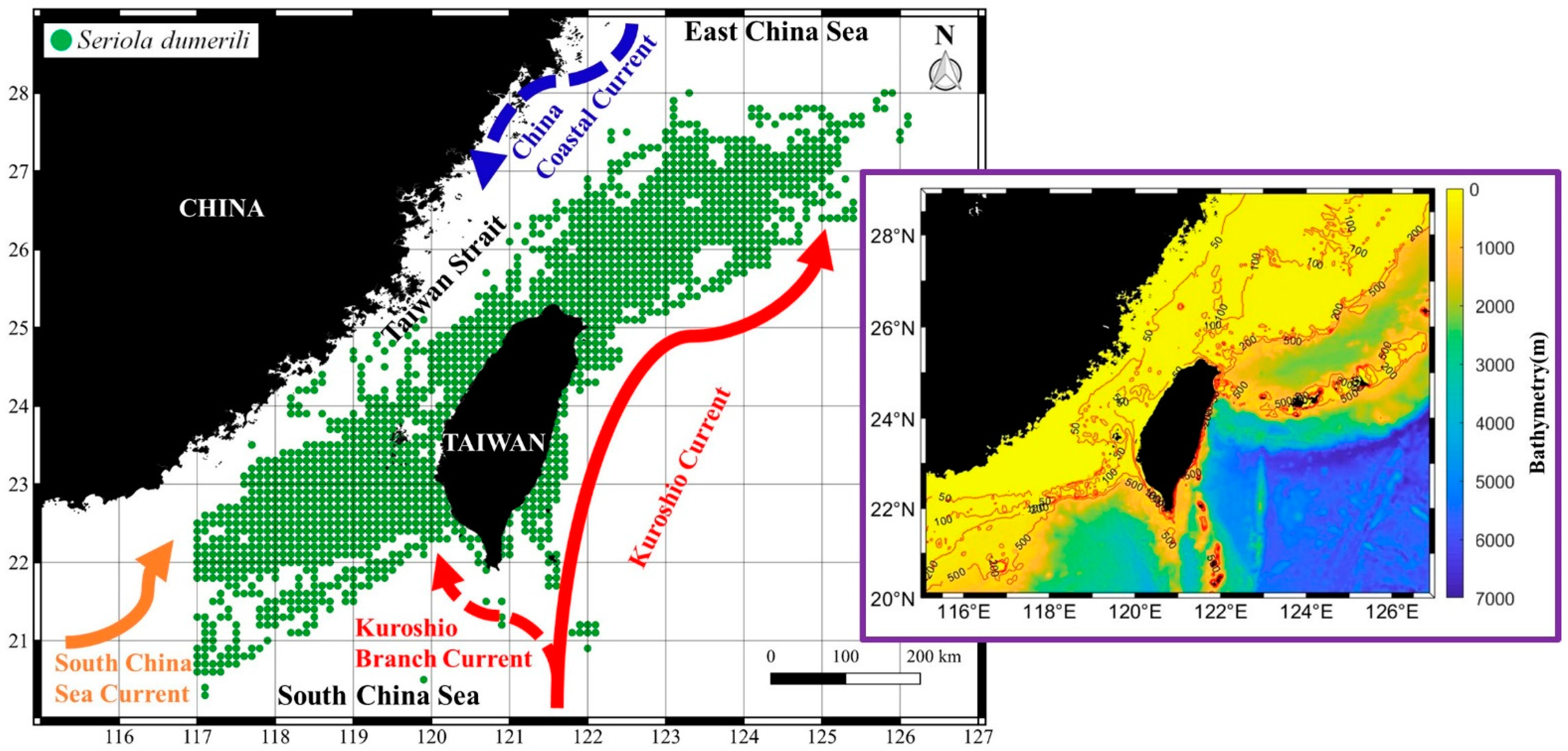
Figure 1. Spatial distribution pattern of S. dumerili caught using angling gear from 2014 to 2017 in the Taiwan Strait (TS). On the right side is a highlighted map of topographic features of bathymetry representing the isobaths, as shown by the orange line.
Remotesensing 14 02932 g001
Figure 2. Seasonal variations and distribution patterns of the fishing locations (in 0.1 spatial grids) of greater amberjack from 2014 to 2017 in the TS.
Remotesensing 14 02932 g002
Figure 3. Monthly average trends in the time series of (a) latitudinal (Lat.) and (b) longitudinal (Lon.) gravitational centers of observed catch rates (G) compared with the monthly average values of (c) sea surface temperature (SST), (d) sea surface salinity (SSS), (e) sea surface height (SSH), (f) chlorophyll-a (Chl-a), (g) mixed layer depth (MLD), and (h) eddy kinetic energy (EKE) in the TS. On the right side is the correlation between latitude and longitude in relation to all the environmental factors.
Remotesensing 14 02932 g003
Figure 4. Seasonal average observed catch rates of S. dumerili overlaid with environmental factors: SST (ad), SSS (eh), SSH (il), Chl-a (mp), MLD (qt), and EKE (ux).
Remotesensing 14 02932 g004
Figure 5. The boxplot graph depicts the GAM and GLM prediction performance based on the root mean square difference (RMSD) value; the model improves if the RMSD value is close to zero.
Remotesensing 14 02932 g005
Figure 6. Estimated environmental variable effects derived from the optimal generalized additive model (GAM) analysis of the catch rates of S. dumerili in the TS: (a) normal quantile–quantile plots, (b) latitude, (c) longitude, (d) SST, (e) SSS, (f) SSH, (g) Chl-a, (h) MLD, and (i) EKE. The solid and black dotted lines indicate the fitted GAM function and 95 percent confidence intervals in (ai). On the x-axis, the rug plot depicts the relative density of data points, while the y-axis depicts the results of smoothing the fitted values. Moreover, s(xn) denotes each model covariate’s spline smoothing function xn.
Remotesensing 14 02932 g006
Figure 7. Three-dimensional partial dependence plots representing the environmental variables with Log (Catch Rates) in the interaction between the (a) SST and SSS; (b) SST and SSH; (c) SST and Chl-a; (d) SST and MLD; (e) SST and EKE in the model.
Remotesensing 14 02932 g007
Figure 8. Seasonal average spatiotemporal distribution pattern of observed catch rates for S. dumerili overlaid with predicted catch rates from selected GAMs in the 2014–2017 period in the TS: (a) spring, (b) summer, (c) autumn, and (d) winter.
Remotesensing 14 02932 g008
Table 1. Satellite-derived remotely sensed oceanographic environmental variables for the data sources and descriptions applied in the model.
Environmental VariablesUnitsData SourceResolution
Sea Surface Temperature (SST)°Chttps://marine.copernicus.eu1/12°
Sea Surface Salinity (SSS)PSUhttps://marine.copernicus.eu1/12°
Sea Surface Height (SSH)mhttps://marine.copernicus.eu1/12°
Sea Surface Chlorophyll-a Concentration (Chl-a)mg/m3oceancolor.gsfc.nasa.gov4.6 km × 4.6 km
Mixed Layer Depth (MLD)mhttps://marine.copernicus.eu1/12°
Eddy Kinetic Energy (EKE)m2/s2https://marine.copernicus.eu1/12°
Table 2. Summary statistics for the building of the GLMs of each variable added and determined using the residual factor. Deviance explained (DE) by the model represented the goodness-of-fit of the model; approximate Akaike information criterion (AIC) was employed to identify the optimal model; are examined to find significant predictors.
VariablesDeviance Explained (%)AICResidual Factorp-Value
Latitude1.726178.84992.59<0.001
Longitude1.476192.58995.14<0.001
SST13.785476.31870.79<0.001
SSS2.946112.02980.31<0.001
SSH2.546133.77984.29<0.001
Chl-a0.116266.091008.9<0.05
MLD0.116266.361008.9<0.05
EKE2.036161.71989.43<0.001
Total Deviance Explained (%)19
Table 3. The contribution of observed catch rates and environmental variables added progressively (first to last) that were retained in the fitted GAMs and determined using the residual factor. DE by the model represented the goodness-of-fit of the model; an approximate AIC value was employed to identify the optimal model. The model’s prediction ability was measured by the determination coefficient (r2) for S. dumerili catch rates in the TS (all p < 0.001).
VariablesDeviance Explained (%)AICResidual Factorp-Value
+s (Latitude)15.15408.49876.34<0.001
+s (Longitude)16.85302.51877.45<0.001
+s (SST)22.94891.28809.42<0.001
+s (SSS)11.55633.03947.86<0.001
+s (SSH)9.755736.73945.99<0.001
+s (Chl-a)5.915959.21957.43<0.001
+s (MLD)2.466154.00995.34<0.001
+s (EKE)2.646134.40982.02<0.001
Total Deviance Explained (%)47.3
r20.47
Table 4. The RMSD reflects the cumulative frequency data test error metric for the observed and predicted high catch rates (>60 percent) of greater amberjack in the TS in 2019.
SeasonObserved Catch RatesPredicted Catch RatesRMSD
Spring3721890.46
Summer3785920.39
Autumn2012390.35
Winter110890.48
Year106111090.42
Publisher’s Note: MDPI stays neutral with regard to jurisdictional claims in published maps and institutional affiliations.