Article

Encoder-Decoder Structure with Multiscale Receptive Field Block for Unsupervised Depth Estimation from Monocular Video

1
School of Mathematics and Computer Science, Wuhan Polytechnic University, No. 36 Huanhu Middle Road, Dongxihu District, Wuhan 430048, China
2
School of Technology, Beijing Forestry University, No. 35 Qinghua East Road, Haidian District, Beijing 100083, China
*
Author to whom correspondence should be addressed.
Remote Sens. 2022, 14(12), 2906; https://doi.org/10.3390/rs14122906
Submission received: 23 April 2022 / Revised: 8 June 2022 / Accepted: 14 June 2022 / Published: 17 June 2022
(This article belongs to the Topic Artificial Intelligence in Sensors)

Abstract

:
Monocular depth estimation is a fundamental yet challenging task in computer vision as depth information will be lost when 3D scenes are mapped to 2D images. Although deep learning-based methods have led to considerable improvements for this task in a single image, most existing approaches still fail to overcome this limitation. Supervised learning methods model depth estimation as a regression problem and, as a result, require large amounts of ground truth depth data for training in actual scenarios. Unsupervised learning methods treat depth estimation as the synthesis of a new disparity map, which means that rectified stereo image pairs need to be used as the training dataset. Aiming to solve such problem, we present an encoder-decoder based framework, which infers depth maps from monocular video snippets in an unsupervised manner. First, we design an unsupervised learning scheme for the monocular depth estimation task based on the basic principles of structure from motion (SfM) and it only uses adjacent video clips rather than paired training data as supervision. Second, our method predicts two confidence masks to improve the robustness of the depth estimation model to avoid the occlusion problem. Finally, we leverage the largest scale and minimum depth loss instead of the multiscale and average loss to improve the accuracy of depth estimation. The experimental results on the benchmark KITTI dataset for depth estimation show that our method outperforms competing unsupervised methods.

Graphical Abstract

1. Introduction

Depth information plays a critical role in the area of robot and computer vision tasks. Low-precision depth may affect the performance of many vision systems, such as 3D reconstruction [1,2], 3D object detection [3,4], autonomous driving [5] and semantic segmentation [6,7]. In this paper, we focus primarily on the depth estimation of monocular images that do not rely on different sensors. However, this is an ill-posed and inherently ambiguous problem because the same 3D scene can be projected to infinitely many 2D images. Obviously, this projection is irreversible.
To address this issue, depth sensors and related algorithms gradually become very popular. However, current methods for depth estimation have the following disadvantages. Depth sensors based on structured light, such as the Microsoft Kinect, are easily disturbed by various conditions of illumination. Additionally, their effect in outdoor environments significantly degrades, and the depth measurement distance is limited [8,9]. Light detection and ranging (LiDAR) can provide accurate 3D information, so it is a reliable scheme for depth perception in outdoor environments. However, sensors based on this technology are cost-prohibitive, and due to the inherent limitation of LiDAR signals, 64 or 128 sparse rotating laser beams can only provide sparse depth maps [4,9]. We plan to infer the depth information of indoor and outdoor scenes using inexpensive, lightweight and conventional cameras based on standard imaging technology. Traditional related algorithms usually start with feature extraction and matching, followed by geometric verification. These methods include box models [10,11,12,13], additional information [14,15,16], nonparametric approaches [17,18,19,20], stereo matching [21,22,23,24,25,26], and SfM methods [27,28,29]. However, these traditional algorithms rely heavily on accurate feature matching, and are hard to guarantee the performance in a real-time manner.
Recent research results utilized deep learning to solve these problems. The main advantage comes from big data, which can help the convolutional neural network (CNN) learn the prior knowledge between objects and their depths. Supervised learning-based methods have been successfully applied to monocular depth estimation [9,30,31,32]. However, to improve the generalization performance of the model, a large corpus of ground truth depth data is usually needed for supervised learning-based methods. In most circumstances, the cost of acquiring ground truth data in real-world scenarios is expensive, limiting the massive growth of datasets. Training on a synthetic dataset [33,34], collecting relative depth annotations [35] or obtaining pseudo ground truth depth maps [36,37] can alleviate the above limitations. Unsupervised learning is another method that has received much attention. These methods only use synchronous stereo pairs [38,39,40,41,42], monocular video [36,43,44,45,46,47,48,49,50], fusion structure from motion (SfM) [51] or optical flow or camera pose [48,52,53] to train the depth estimation model without any depth data. However, stereo vision requires offline calibration, monocular video is affected by illumination and occlusion, and the optical flow approach requires additional networks.
To this end, we recover the dense depth of monocular images under three challenging conditions. The first condition is that no 2D or 3D ground truth information is available. The second condition is that no input image from other perspectives enables triangulation. The third condition is that the photometric loss is highly influenced by illumination and occlusion. To address these challenges, we design a novel pose CNN to assist the training of a depth map inference network with encoding and introduce the largest scale loss to enhance the inference accuracy. Overall contribution of our research summarizes as below:
(1) According to the SfM theory, we propose a novel depth CNN model for depth map inference by a given video sequence, no other depth maps or rectified stereo pairs are needed and our pose CNN also outputs two confidence masks to reduce the effect of occlusion.
(2) We propose a new efficient upsample block with a channel-wise attention mechanism that supports our network to achieve better performance without multiscale supervision and employ a novel optimizer [54,55] to improve the convergence speed.
(3) Our method is evaluated on the KITTI dataset [56] and achieves the best depth estimation performance. Furthermore, our method is generalized to unknown environments to demonstrate its superiority.
The rest of the paper is arranged as follows. In Section 2, the proposed unsupervised learning method and detailed implementation process is given. Experimental comparison and analysis are given in Section 3, and finally, the discussion and conclusion of our work are given in Section 4.

2. Method

Our method combines training a single view depth and pose estimation network from unlabeled monocular video sequences and uses the largest scale loss to constrain them to predict depth. We assume that most of the scenes we are interested in are rigid. First, borrowing the camera coordinate transformation and traditional SfM method, we describe the key ideas behind our depth prediction framework. Second, we analyze the role of each component of our method. Finally, we present how the CNN parameters are learned in a self-supervised way.

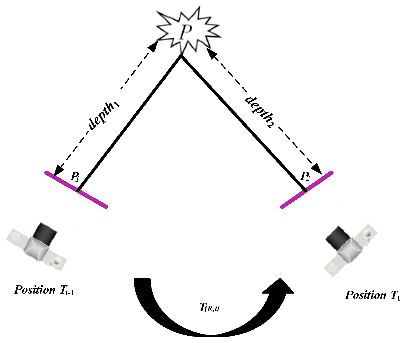
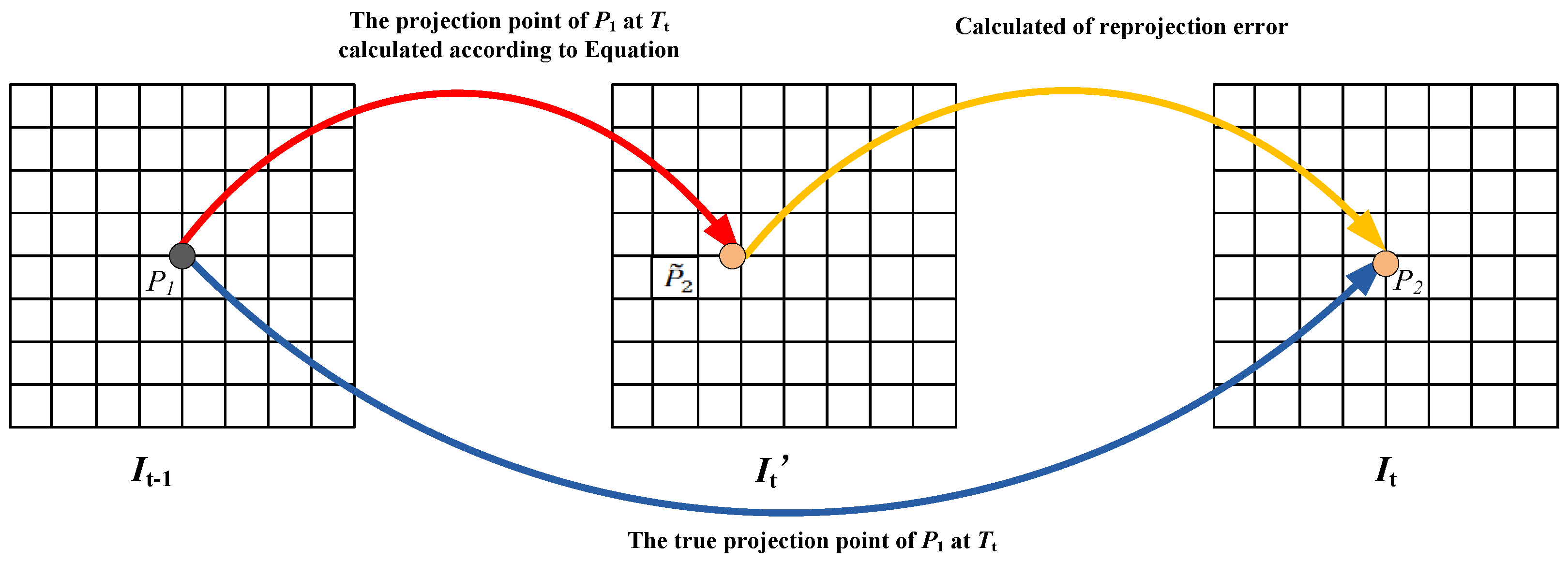
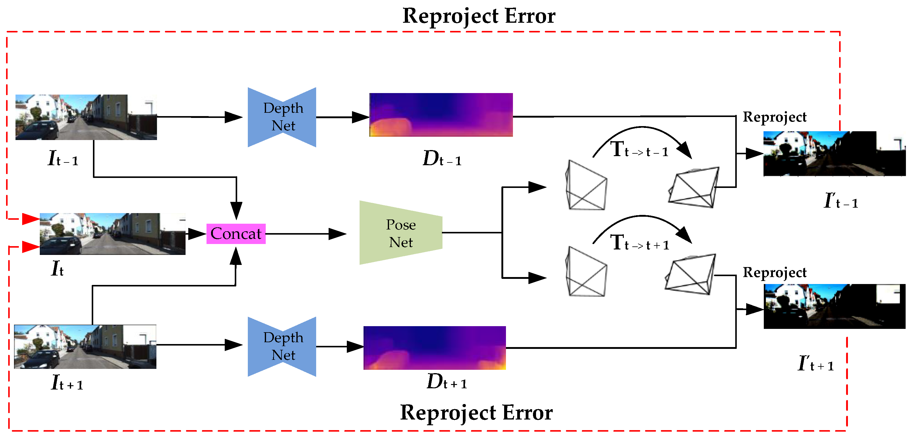
2.1. Reprojection Error

The ideal projection imaging model reflects the projection relationship from the object to the image plane in 3D space. For any point P(xw,yw,zw) in the real world, after passing through the pinhole camera, the pixel coordinates projected to the imaging plane are P(u,v); then, according to the pinhole imaging model [57], we have,
Z P ( u , v ) = Z ( u v 1 ) = K [ R P ( x w , y w , z w ) + t ] = K T ( R , t ) P ( x w , y w z w )
where Z is the distance from P(xw,yw,zw) to the camera, K is the camera internal parameters, R is a rotation matrix, t is a translation vector, and T(R,t) is the conversion matrix composed of R and t, called camera extrinsic parameters. Equation (1) describes the projection relationship from the world coordinates to the pixel coordinates.
As illustrated in Figure 1, for a monocular camera, we assume that the projection points of P(xw,yw,zw) on the imaging plane (purple line) are P1 and P2 at Tt−1 and Tt, respectively. From Equation (1), we can obtain,
{ d e p t h 1 P 1 ( u , v ) = K T 1 P ( x w , y w , z w ) d e p t h 2 P 2 ( u , v ) = K T 2 P ( x w , y w , z w )
If the conversion matrix of the camera moving from the position at time Tt−1 to the position at Tt is T(R,t) and the world coordinate system coincides with the camera coordinate system at Tt−1, then we can obtain,
d e p t h 2 P 2 ( u , v ) = K T ( R , t ) d e p t h 1 K 1 P 1 ( u , v )
Since the homogeneous coordinates are multiplied by nonzero constants to express the same meaning, after normalizing the pixel coordinates, we obtain,
P ˜ 2 ( u , v ) = K T ( R , t ) d e p t h 1 K 1 P 1 ( u , v )
Equation (4) describes the mapping relationship between the pixel coordinates of adjacent frames. As illustrated in Figure 2, we can calculate the pixel coordinate P ˜ 2 of P1 at Tt, which means that given two adjacent frames of images It−1 and It, we can obtain the image It from It−1 and further construct the reprojection error of the two adjacent frames,
r e p r o j _ e r r o r = | | I t I t | |
Therefore, we can design neural networks to output depth and camera pose information to optimize the reprojection error.

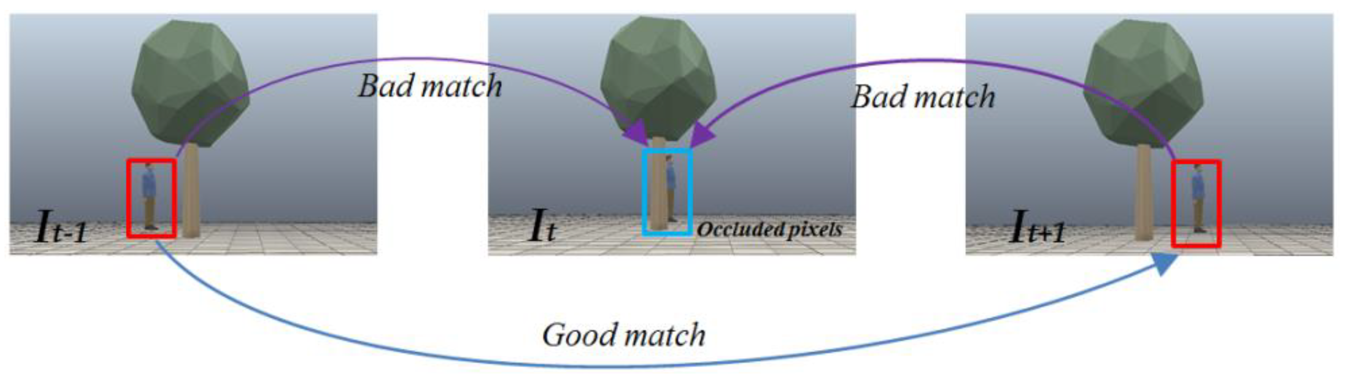
2.2. Occlusion Error

For monocular video sequences, occlusion between adjacent frames is common. A typical occlusion error is shown in Figure 3, where It−1, It and It+1 are three frames of an image at adjacent moments. In these images, a pedestrian is obscured by a tree at time t and not obscured by a tree at time t − 1 and t + 1. From Equations (4) and (5), we know that the pixel matching between the red and blue areas is poor, and the matching between the red areas is good. Therefore, we can design neural networks to output confidence masks to mask out occluded pixels when optimizing the reprojection error.

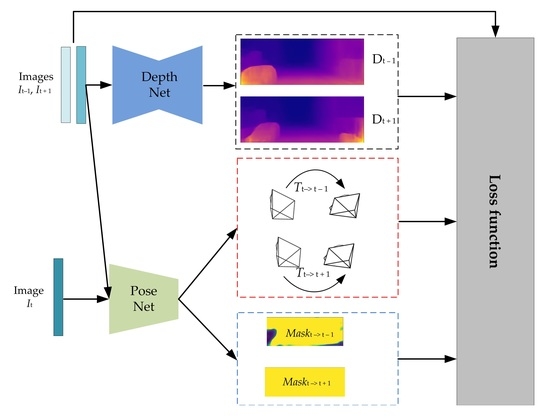
2.3. Neural Network Model

Our method is designed to train depth, ego-motion and mask networks using unsupervised learning from monocular video, where the supervision signal comes from the unlabeled video sequence itself and does not depend on any depth information. The full framework of this method is shown in Figure 4. Although the depth prediction and the pose estimation network need to be jointly trained, these models can be used independently during test inference. The input to our networks is three adjacent RGB images It−1, It and It+1. We first use the depth estimation mode to output the corresponding depth maps Dt−1 and Dt+1 and then predict the relative 6D camera poses Ttt−1 and Ttt+1 using the pose estimation mode. From Equations (4) and (5), we can jointly train the depth and pose estimation networks.

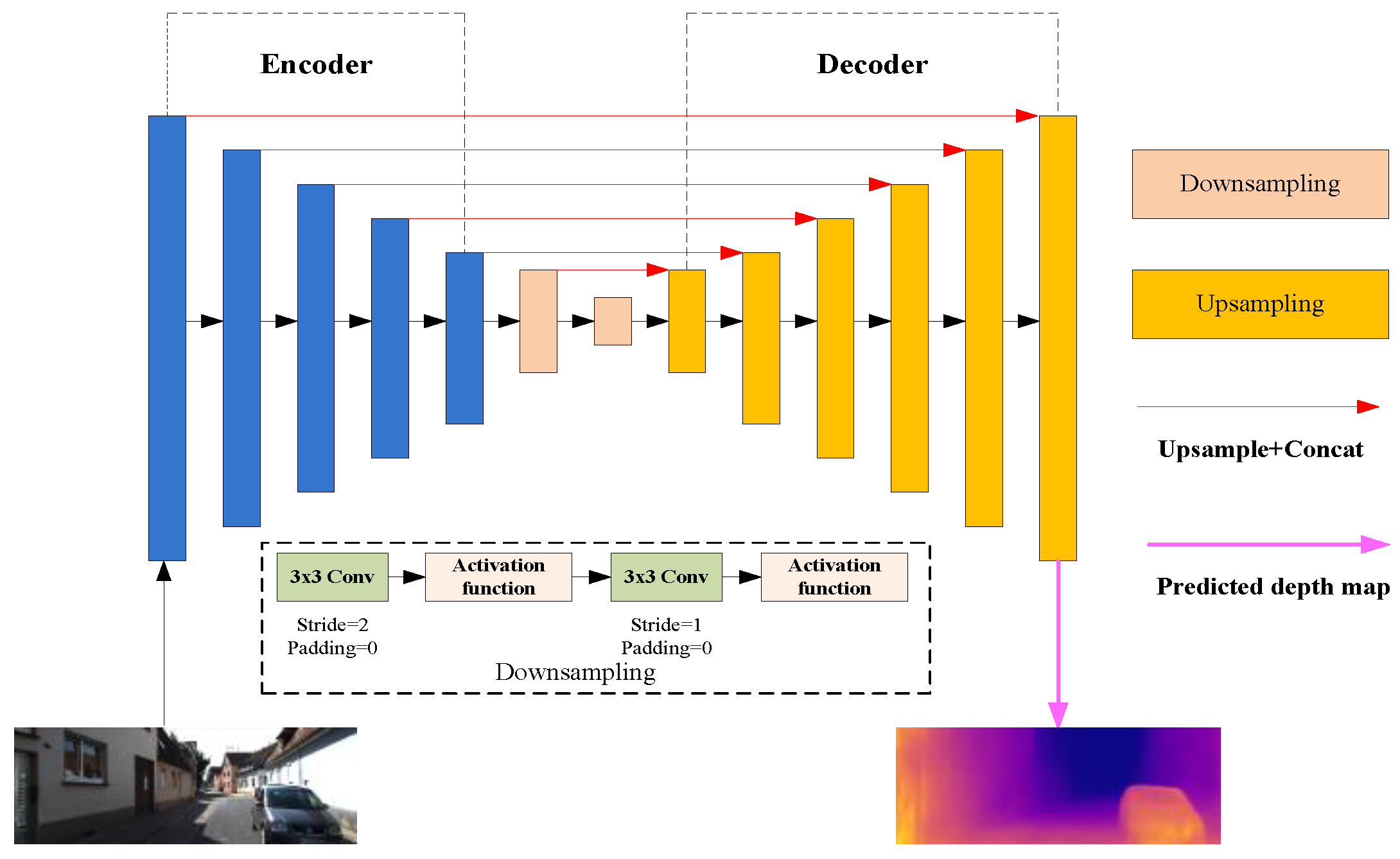
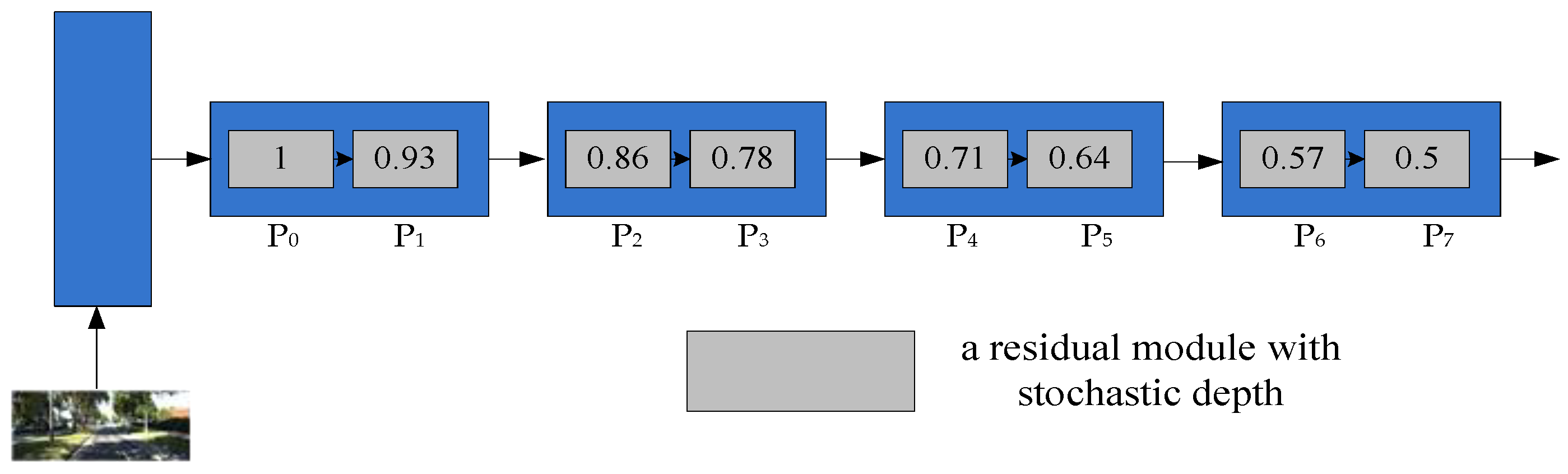
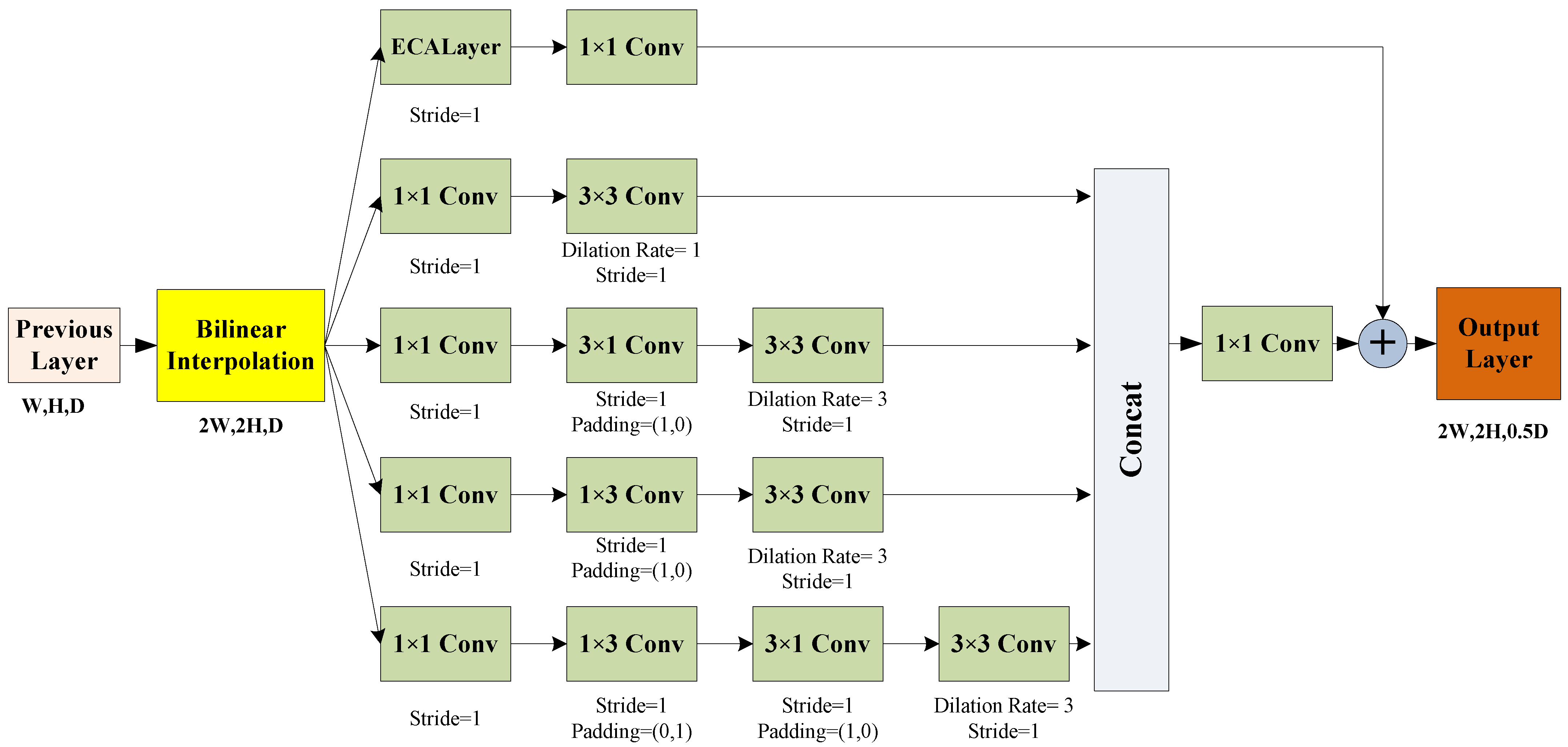
2.3.1. Depth Estimation Network

We propose to solve the depth prediction for monocular images as a disparity map regression learning problem. The difference from previous related work [39,43,44,45,47,52,57] is that the output of the network only contains a single-scale depth map, not a multiscale depth map. Our depth estimation network is visualized in Figure 5. For the encoder, the most representative features are automatically extracted through our backbone network model, which is based on deep networks with stochastic depth [58] because it can reduce the training time to improve performance. For the decoder, a series of upsampling with attention structures and asymmetric convolution kernels are used to gradually restore the resolution of the output feature map. Two downsampling layers build a bridge between the encoder and decoder modules, including two 3 × 3 convolution layers with activation function, which focus on reducing the size of the feature map and keeping the channel constant. Some short-cut connections (red arrows) are also added between corresponding layers in the encoder and decoder to enhance the information flow. Finally, the output of the network goes through a 3 × 3 convolutional layer and a sigmoid layer to predict the disparity map.
ResNet [59] is the first choice for previous unsupervised depth estimation tasks [34,39,40,42,43,45,49,52,53]. In the process of training ResNet, stochastic dropping of hidden nodes or connection layers (the most common is the dropout method [60]) does not affect the convergence of the algorithm, which shows that ResNet has good redundancy. For fairness of comparison, we improved ResNet while keeping the number of convolution layers unchanged, which can not only reduce the parameters, but also improve the accuracy of depth estimation. Inspired by [58] and [59], we design an 18-layer stochastic residual structure (StoResNet-18) as the backbone network. A typical residual module is shown in Figure 6a, which can be defined as,
Y = F(X) + X
when considering multiplying each hidden activation by an independent Bernoulli random variable b ∈ {0,1}, we can extend the typical residual module to a residual module with stochastic depth (see Figure 6b), which can be defined as,
Y = b × F(X) + X,
In our research, StoResNet-18 is similar to ResNet-18 except for the residual module and discards the fully connected layer. Therefore, we also divide StoResNet-18 into 5 layers according to the output size, and each layer contains two residual blocks with stochastic depth except for the first layer. The probability of stochastic dropping of hidden nodes at each layer is shown in Figure 7, where Pl is the probability value when b = 1 in the l-th residual module with stochastic depth (see gray square), which can be defined as,
P l + 1 = P ( b = 1 ) = { P l P 0 P 7 M a x ( l )   0 < l < 7 , 0.5   l = 7 , 1   l = 0 .
It should be emphasized that b = 1 remains unchanged during testing to reduce the network depth during training while maintaining the full depth at testing time.
Our decoding module is almost symmetrical to the encoding and mainly composed of six new upsampling structures, mainly to linearly increase the resolution of the output. Inspired by the idea of the inception module with dimension reductions [61], asymmetric convolution kernel can be reducing the number of network parameters and improve the speed of network convergence compared with symmetric convolution kernel. According to this discovery, we design an upsampling structure with channel attention and asymmetric convolution kernels. By fusing both the feature from the previous phase and the corresponding phase in the encoder module as the output of each phase, and using the new upsampling structure to improve the resolution of the output. This can be observed in Figure 8. First, we use bilinear interpolation to double the size of the output feature map of the previous layer while maintaining the same channels. Next, we use a multiscale receptive field structure to help extract detailed feature information. To keep the size of the receptive field constant while reducing the inference time, we use a 3 × 3 dilated convolution kernel instead of a 5 × 5 convolution kernel and an asymmetric convolution kernel (such as 1 × 3 and 3 × 1). Finally, we introduce the channel attention mechanism-ECALayer [62] to overcome the paradox of performance and complexity trade-off. Detailed parameters and structure are shown in Figure 8.

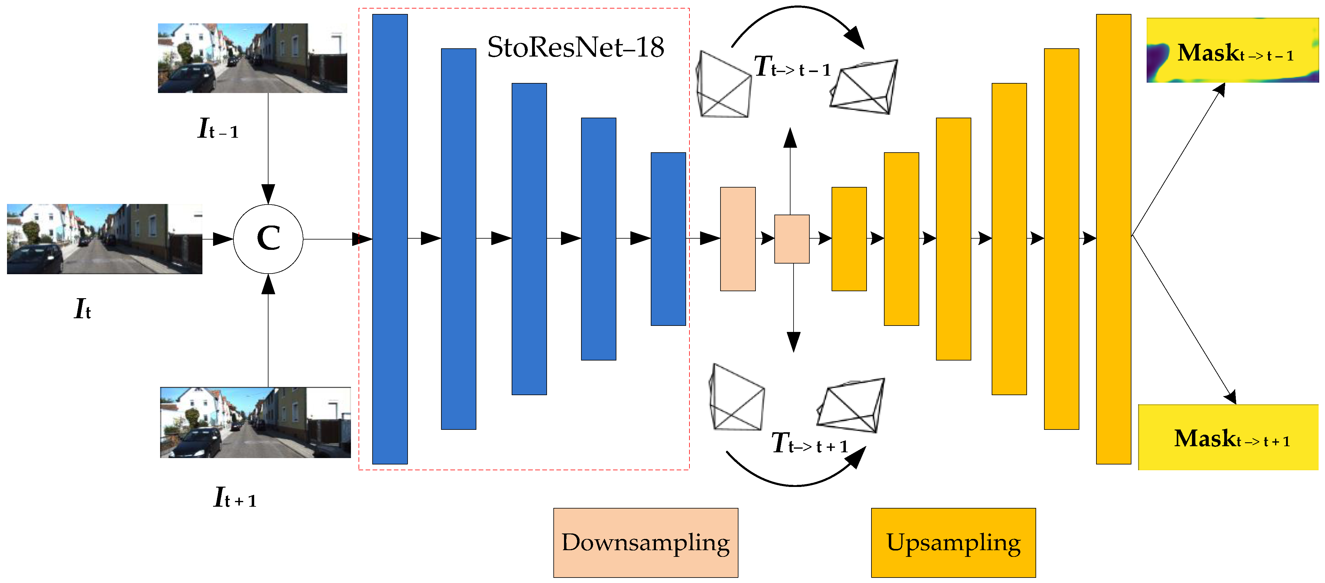
2.3.2. Pose and Mask Estimation Network

Figure 9 shows a schematic layout of the pose and mask estimation networks with concatenated three adjacent frames (It−1, It, It+1) as input and the predicted mask map and relative poses as output. Three input images first pass through the StoResNet-18 feature extractor, which computes feature maps at five output resolutions (scale of 1/2, 1/4, 1/8, 1/16 and 1/32) and then continues to reduce (scale of approximately 1/64 and 1/128) through two downsampling layers. In the first stage, we output two 6-DoF relative poses (Ttt−1 and Ttt+1). Similar to the depth estimation network, in the second stage, we first use six upsampling structures to restore the resolution of the output feature map from the first stage and then use a sigmoid layer to output our predicted mask.

2.4. Data Preprocessing and Augmentation

Since a moving object violates the assumption of a static scene in error reconstruction, we follow Zhou et al.’s [43] and Bian et al.’s [45] preprocessing method to remove all static frames from the test scenes. A large quantity of training data is a prerequisite for achieving an accurate model. To improve the generalizability and robustness of our unsupervised learning model, we transform the training data by random operations performed spontaneously. It is worth noting that the camera internal parameters also need to be changed when the sequence of images is transformed. The augmentation methods are described as follows:
Flip: Input sequences of video are horizontally flipped with a 0.5 probability.
Translation: Input sequences of images are scaled by a random number t ∈ [1, 1.15] and cropped to keep the same initial size.

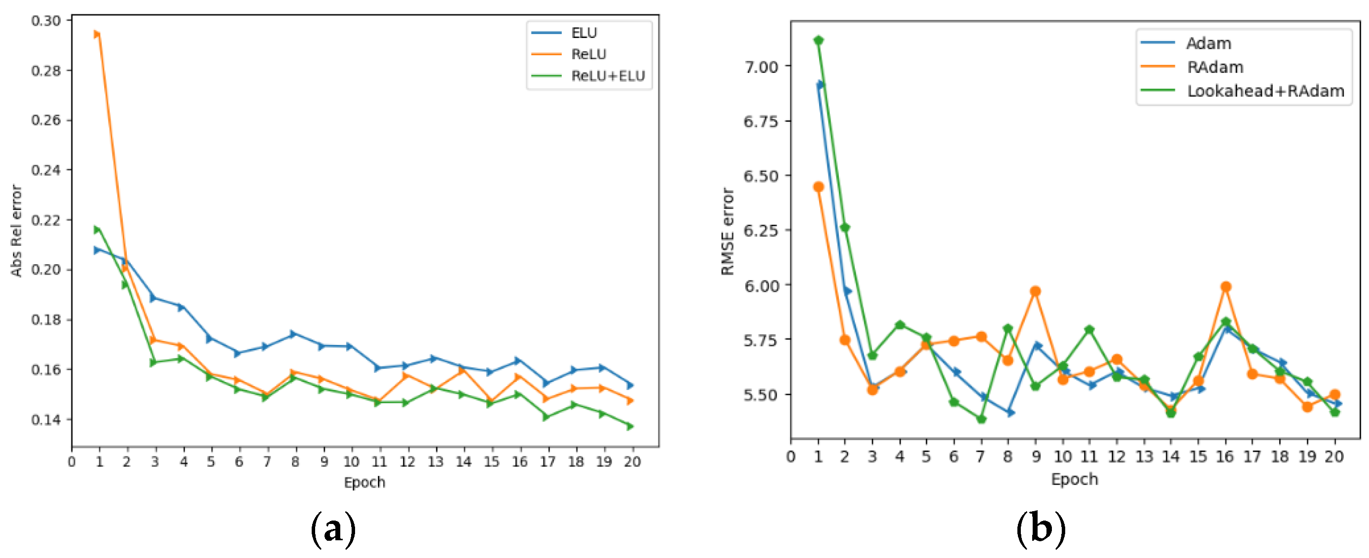
2.5. Optimizer and Activation Function
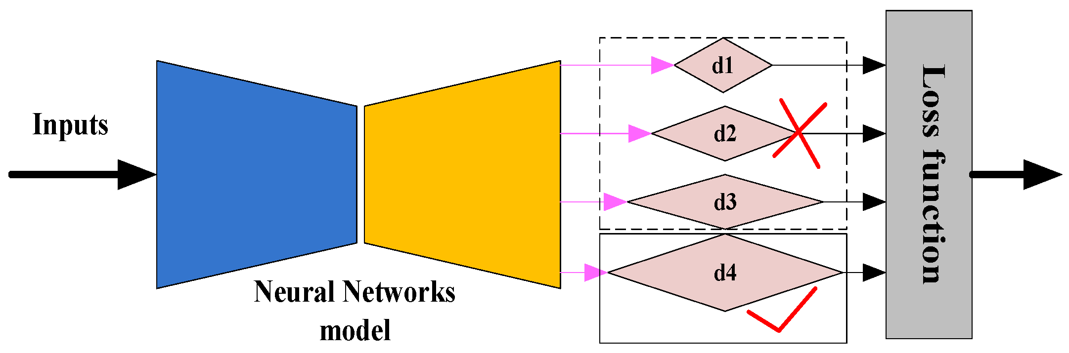
Fast and stable optimization algorithms are the goal that researchers have been pursuing. Previous related work [39,40,42,43,44,47,49,52,53] mainly used the adaptive optimization algorithm (Adam) [63], which is the first choice for training depth estimation models. Adam is a stochastic objective function algorithm based on a first-order gradient, which works well with sparse gradients and in online and nonstationary settings. Although the Adam method shows a quick convergence rate, it easily falls into a local optimal solution. We introduce a novel variant of Adam called RAdam [54]. Compared with the Adam method, RAdam can improve the robustness of model training and adapt to different learning rates over a broader range. We further introduce a new optimization algorithm called Lookahead [55], which uses any standard optimizer in its internal loop to update the “fast weights” k times and then updates the “slow weights” once in the direction of the final fast weights. By using Lookahead with RAdam optimizers, we can achieve faster convergence of the model with less overhead.
For the nonlinear activation function in our network, we use exponential linear units (ELUs) [64] to replace the rectified linear units (ReLUs) [65] excluding StoResNet-18. Although ELU and ReLU have been widely used in other similar works [40,42,43,45,52], we found that only using ELU will prematurely make the network fall to a local minimum value, making subsequent improvement difficult. When ReLU is used instead of ELU in StoResNet-18, the depth prediction accuracy is further improved. Training lasts for approximately 20 epochs in total on the KITTI dataset [56] (see Section 3.1) to verify the convergence of the combination of different optimization and activation functions.
We use the activation function as a single variable for experimentation, and the results are shown in Figure 10a. We find that the combination of ReLU and ELU can reduce the absolute average relative (Abs Rel) error. Meanwhile, we also use optimization functions as a single variable to conduct experiments for experimentation, and the results are shown in Figure 10b. Obviously, the combination of Lookahead and RAdam achieve the best results in terms of the root mean squared error (RMSE).

2.6. Loss Function

Our goal is to combine ego-motion networks to train depth estimation networks using monocular video sequences. Similar to [38,39,40,43,45], we formulate the depth prediction problem as the minimization of synthesizing new viewpoint errors at the training time. In addition, we choose the largest scale supervision instead of the multiscale supervision [39,43,44,45,47,52,57], see Figure 11.
First, It−1, It and It are three adjacent RGB images used as the input of the pose estimation network, Mφ denotes the confidence masks to mask out the invalid pixels when It−1 is reprojected to It and It+1 is reprojected to It, A is a tensor with elements of 1, and the scale is the same as Mφ. In our task, the element value in Mφ can only be 0 or 1, so we can use binary cross entropy to construct the first loss function,
L o s s M a = 1 N φ { t > t 1 , t > t + 1 } [ A log ( M φ ) + ( 1 A ) log ( 1 M φ ) ]
where φ ∈ {t−>t−1, t−>t+1} and N is the number of validity pixels. From Equation (5), we know that our goal is to minimize the reprojection error. The structural similarity index metric (SSIM) [66] and Manhattan distance are better choices to judge the similarity of images, which are used together to solve the gradient locality problem in pose estimation and to eliminate the discontinuity of learning depth in low texture regions. If re_error(t−>t−1) and re_error(t−>t+1) are the reprojection errors of It−1 and It+1 reprojected to It, respectively, in our research, we use the minimum error min(re_error(t−>t−1), re_error(t−>t+1)) instead of the average error mean(re_error(t−>t−1) + re_error(t−>t+1)). Therefore, we have,
L o s s P e = 1 N φ { t > t 1 , t > t + 1 } m i n ( M φ [ α 1 S S I M ( I t , I ˜ φ ) 2 + ( 1 α ) | I t I ˜ φ | ] )
The simplified formula of SSIM is,
S S I M ( I t , I ˜ φ ) = [ 2 μ ( I t ) μ ( I ˜ φ ) + C 1 ] [ 2 σ ( I t , I ˜ φ ) + C 2 ] [ μ ( I t ) 2 μ ( I ˜ φ ) 2 + C 1 ] [ σ ( I t ) 2 σ ( I ˜ φ ) 2 + C 2 ]
where I ˜ φ represent It−1 and It+1 reprojected to It, respectively, φ ∈ {t−>t−1, t−>t+1}, μ(.) and σ ( . ) calculate the average value and standard deviations of corresponding images, respectively, C1 and C2 are small constants to prevent the denominator from being zero in Equation (11), and α is a weighted value. We empirically set α = 0.85 in our task.
Due to the photometric loss, it is not possible to provide sufficient information in low-texture or homogeneous areas [45], and depth discontinuity usually occurs on the image gradient. Therefore, we use the image-aware smoothness formulation to weight the gradient of the image depth,
L o s s S m = 1 N φ { t > t 1 , t > t + 1 } ( | D t | e 1 N | I t | + | D φ | e 1 N | I φ | + | D φ | e 1 N | I φ | )
where ∇ denotes the 2D differential operator along spatial directions and Dt and Dφ are depth maps.
Our final objective function can be expressed as,
L o s s = α L o s s M a + β L o s s P e + γ L o s s S m
We set α = 0.2, β = 1.0 and γ = 0.1. Table 1 reports the results of the multiscale and largest scale supervision on the KITTI dataset. We find that the largest scale supervision method is better.

3. Experimental Result

In this section, we evaluate our method based on common metrics and protocols adopted by prior methods and compare them with existing depth estimation approaches. We use the public dataset KITTI [56] as a benchmark to verify the validity of our model. The method is implemented using the PyTorch framework [67], which is a machine learning toolkit released by Facebook that can run on graphics processing units (GPUs) to achieve acceleration. It is worth noting that our model trains short depth networks but uses full deep networks during testing.

3.1. Training Datasets and Details

KITTI: The KITTI dataset is mainly captured by cameras and laser sensors on a standard station wagon. A total of 42,382 stereo pairs with a size of 375 × 1242 from 61 scenes in the “residential”, “road” and “campus” categories constitute our original dataset. In our research, we follow the data preprocessing method of Zhou [43] and Bian et al. [45] and exclude all static sequence frames whose average optical flow size is less than 1 pixel in the original dataset and downsample the image to 128 × 416. As a result, we finally obtain 38,758 images for training and 5464 images for validation. To make a fair comparison with related work [38,39,40,43,45,52,57], we use an Eigen split [30] to evaluate the depth estimation performance of 697 images in two different depth ranges: 0−80 m and 0−50 m. Note that our model is trained on a network with stochastic depth, but we use full depth during testing.
According to [43], we use segments of three adjacent consecutive video frames as the input of networks, in which the middle image is set as the reference frame to calculate the loss together with the adjacent two images. During training, we perform data augmentation online and use ELU activation except for StoResNet-18 with a batch of size 4 and initialize the StoResNet-18 parameters via the pretrained classification model on ILSVRC 2012 [68]. In addition, we use the combination of RAdam with β1 = 0.9, β2 = 0.999, Lookahead with k = 5, α = 0.5 as the optimizer, and the learning rate r = 1 × 10⁻⁴, which remains unchanged because we find that the experimental results do not improve significantly when fine-tuning the parameter r. Our depth estimation model is trained on GeForce 2080Ti GPUs for approximately 20 epochs.
Figure 12 shows the detailed visual results of the KITTI datasets. Compared with other unsupervised methods [43,45], our method shows better results on small objects and boundaries.

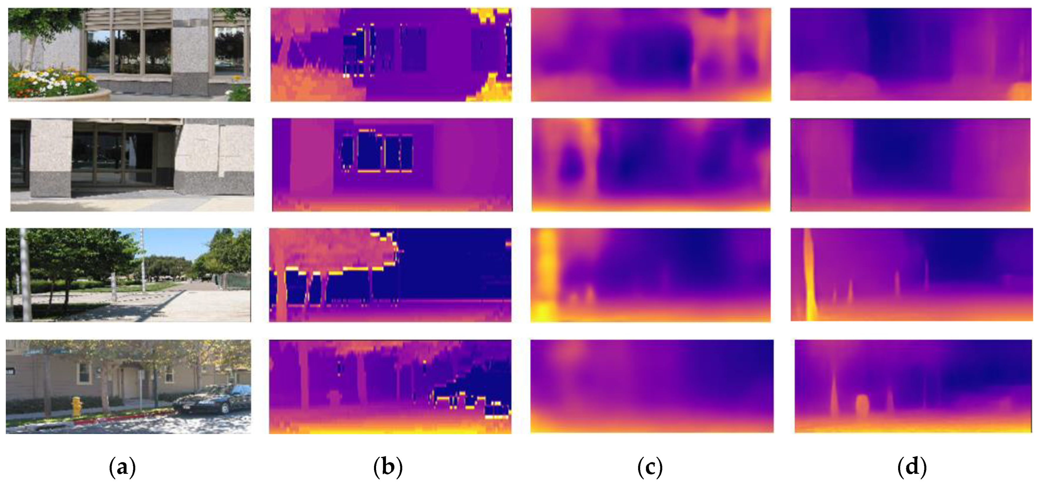
3.2. Generalization on Make3D Dataset

Make3D: The Make3D dataset of campus scenes is collected and contains 400 training and 134 testing images. Since there is no video sequence image, our method cannot train on the dataset. However, to evaluate the generalization ability of our method in unknown environments, we apply the depth estimation model trained on the KITTI dataset to the Make3D dataset for testing. Figure 13 visualizes some generalized depth images. Our method performs quite well, such as restoring detailed information about tree trunks, utility poles and fire hydrants.

3.3. Evaluation Criteria

For the depth estimation task, we adopt the following standard evaluation metrics, which are similar to [30,38,39,40,43,44,45,52,57], to quantitatively assess the performance of our method. There are several categories:
  • Mean absolute relative error (Abs Rel): 1 | N | p i N | D ( p i ) D ^ ( p i ) | D ( p i )
  • Mean square relative error (Sq Rel): 1 | N | p i N ( D ( p i ) D ^ ( p i ) ) 2 D ( p i )
  • Root mean squared error (RMSE): 1 | N | p i N ( D ( p i ) D ^ ( p i ) ) 2
  • Root mean squared error log scale (RMSElog): 1 | N | p i N ( log D ( p i ) log D ^ ( p i ) ) 2
  • Threshold accuracy: 1 | N | p i N | { D ^ ( p i ) : max ( D ( p i ) D ^ ( p i ) , D ^ ( p i ) D ( p i ) ) } = δ < t h r e s h o l d |
Here, D(pi) and D ^ (pi) denote the ground truth and estimated depth values, respectively, corresponding to pixel pi, N is the set of validated pixels, and the threshold is a constant of 1.25, 1.252 or 1.253.
We report the experimental results on the KITTI dataset in Table 2, where our method is superior to other state-of-the-art methods when compared with networks trained on monocular video sequences. Recently, some related works jointly learned multiple tasks (i.e., optical flow) [52,53] or calibrated stereo pair images (i.e., pose supervision) [38,39,40], while our method does not need to do so. This effectively reduces the training and reasoning overhead. Table 2 shows the results on the KITTI dataset.
Furthermore, we quantitatively compare the generalization ability of the model on the Make3D dataset. Since the sizes of images are different from KITTI, we perform center cropping on these images and resize them to 128 × 416, following the evaluation strategy used by Godard [39]. Table 3 summarizes the results on the Make3D dataset. Our method shows better generalization ability than previous methods.

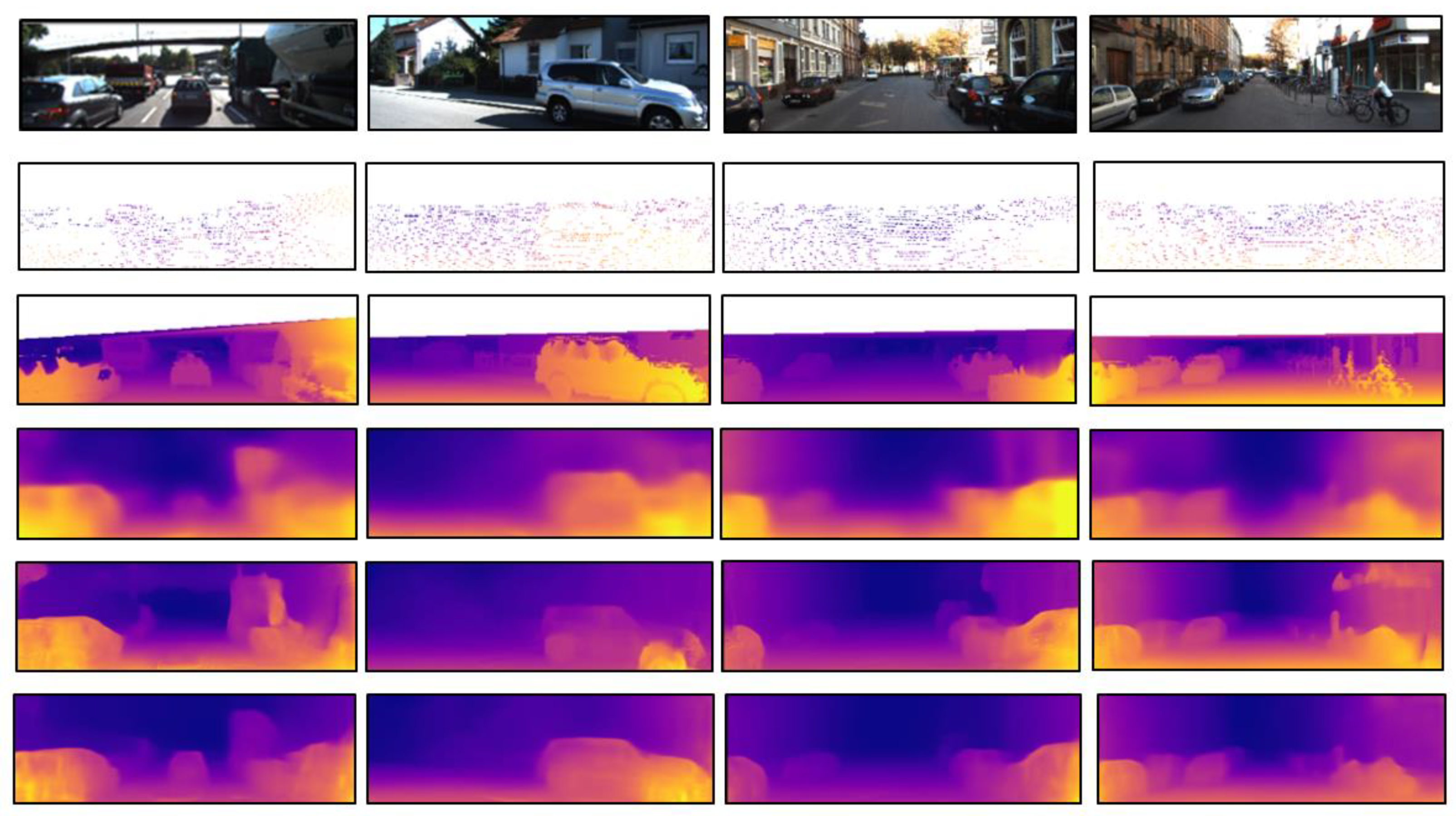
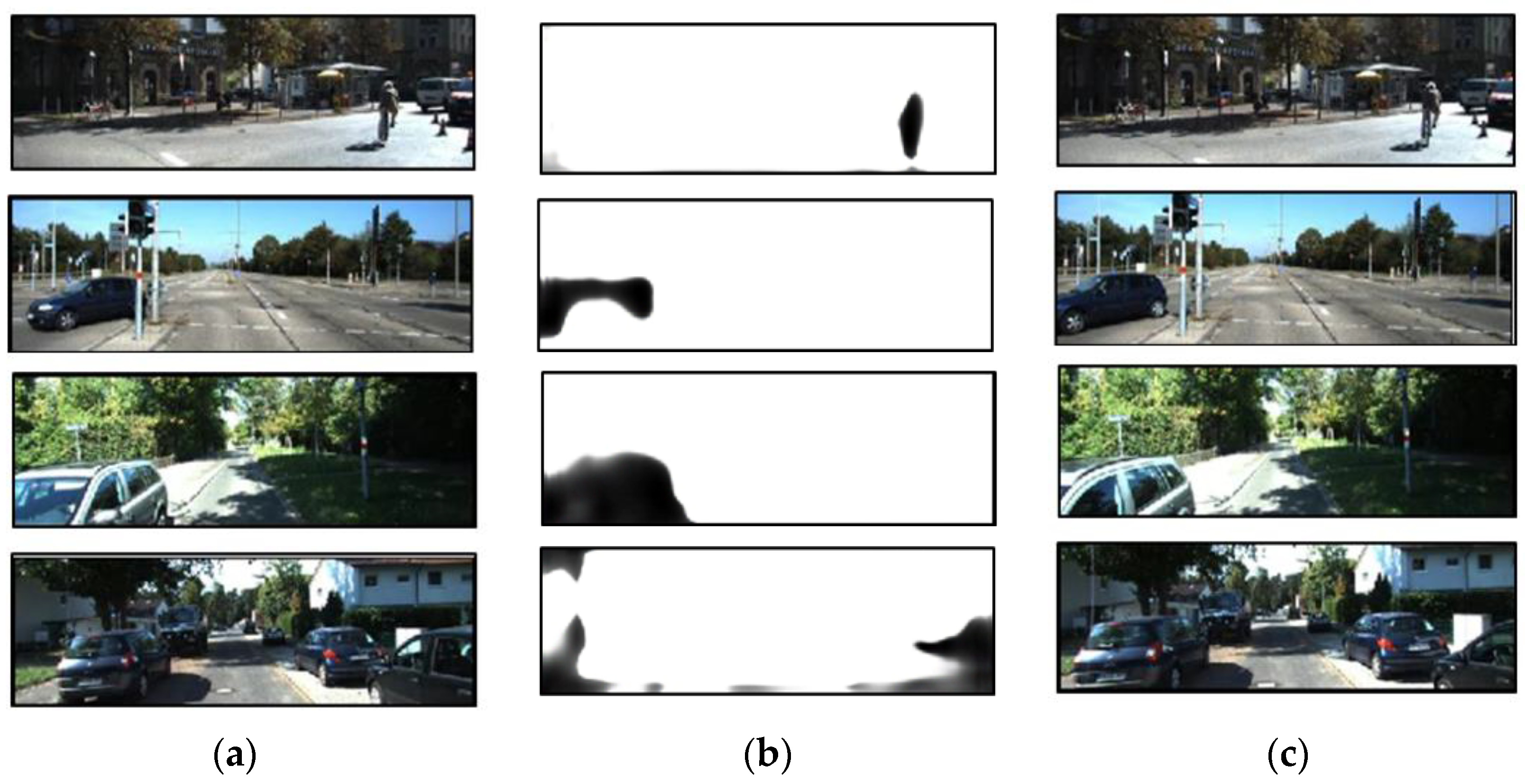
3.4. Confidence Mask Visualization

Figure 14 shows the visualization result of the confidence mask. It−1 and It are two frames of the image at adjacent moments. From Equation (4) and Section 2.2, we know that the calculated reprojection error will be invalid when there are occluded or moving objects in the scene. Therefore, we need to mask out the occluded or moving objects to optimize the reprojection error in the process of training the depth estimation network. In contrast with previous related work [37,50], our method does not require pre-segmentation of moving objects to obtain the confidence mask. Figure 14b denotes the confidence mask output by our method, where the black area is the region where two adjacent frames have occlusion or motion during reprojection. The result also shows that the visual results of the confidence mask output by our method are generally consistent with our expected results.

4. Conclusions

We recover the depth information of monocular images under three challenging conditions. The first is that there is no real depth information for reference; the second is that no input images from other angles can be triangulated; and the third is that the photometric reconstruction loss is greatly affected by illumination and occlusion. To solve these challenges, we design a new camera pose network to assist the training of the depth estimation network and introduce the largest scale loss to improve the prediction accuracy. First, according to SfM theory, we treat depth prediction as a disparity map regression problem and propose a new deep CNN structure to train our depth estimation model without other depth maps or rectified stereo image pairs. Furthermore, we output two confidence masks to reduce the impact of occlusion. Finally, we present a new upsampling structure with a multiscale receptive field to support the training of our network using the maximum scale loss function. Experimental results show that our method is more accurate than competing methods on KITTI datasets.
Our method produces accurate and detailed depth map from monocular video. However, even though our method predicts two confidence masks to address occlusion error, the accuracy of depth estimation will decrease in dynamic scenes, especially when there are a large number of moving objects. Our method also highly depends on the photometric consistency between adjacent frames, which also means that illumination has a great impact on our results. Our method must be performed under the condition that the camera intrinsic parameters are obtained in advance, but it is not easy to obtain the camera intrinsic of datasets in real scenes.
In future work, we will focus on unsupervised monocular depth learning method in dynamic scenes with unknown camera intrinsic and improve the robustness of our method. We will also apply the method to other useful applications, such as 3D SLAM, 3D reconstruction, 3D object recognition and semantic segmentation.

Author Contributions

S.C.: writing—original draft, methodology, visualization, investigation, validation, formal analysis. J.H.: conceptualization, methodology, writing—review and editing, M.T.: conceptualization, supervision, funding acquisition. R.D. and J.K.: supervision, methodology, writing—review and editing. All authors have read and agreed to the published version of the manuscript.

Funding

This work was funded by the National Natural Science Foundation of China (Grant number 32071680); Science and Technology Department of Henan Province (Grant number 182102110160); Young Teachers Found of Xinyang Agriculture and Forestry University (Grant number 201701013); Key-Area research and development program of Guangdong province (Grant No. 2019B020223003); Fundamental Research Funds for the Central Universities (Grant No. 2021ZY72).

Data Availability Statement

Not applicable.

Conflicts of Interest

The authors declare that they have no known competing financial interests or personal relationships that could have appeared to influence the work reported in this paper.

References

  1. Tulsiani, S.; Gupta, S.; Fouhey, D.; Efros, A.A.; Malik, J. Factoring Shape, Pose, and Layout from the 2D image of a 3D scene. In Proceedings of the IEEE Conference on Computer Vision and Pattern Recognition (CVPR), Salt Lake City, UT, USA, 18–23 June 2018; pp. 302–310. [Google Scholar]
  2. Gupta, S.; Arbelaez, P.; Girshick, R.; Malik, J. Aligning 3D models to RGB-D images of cluttered scenes. In Proceedings of the 2015 IEEE Conference on Computer Vision and Pattern Recognition (CVPR), Boston, MA, USA, 7–12 June 2015; pp. 4731–4740. [Google Scholar]
  3. Xu, B.; Chen, Z. Multi-level Fusion Based 3D Object Detection from Monocular Images. In Proceedings of the 2018 IEEE/CVF Conference on Computer Vision and Pattern Recognition (CVPR), Salt Lake City, UT, USA, 18–23 June 2018; pp. 2345–2353. [Google Scholar]
  4. Wang, Y.; Chao, W.; Garg, D.; Hariharan, B.; Campbell, M.; Weinberger, K.Q. Pseudo-LiDAR From Visual Depth Estimation: Bridging the Gap in 3D Object Detection for Autonomous Driving. In Proceedings of the IEEE Conference on Computer Vision and Pattern Recognition (CVPR), Long Beach, CA, USA, 15–20 June 2019; pp. 8445–8453. [Google Scholar]
  5. Sun, L.; Yang, K.; Hu, X.; Wang, K. Real-time Fusion Network for RGB-D Semantic Segmentation Incorporating Unexpected Obstacle Detection for Road-driving Images. IEEE Robot. Autom. Lett. 2020, 5, 5558–5565. [Google Scholar] [CrossRef]
  6. Hu, X.; Yang, K.; Fei, L.; Wang, K. ACNet: Attention Based Network to Exploit Complementary Features for RGBD Semantic Segmentation. In Proceedings of the 2019 IEEE International Conference on Image Processing (ICIP), Taipei, China, 22–25 September 2019; pp. 1440–1444. [Google Scholar]
  7. Deng, L.Y.; Yang, M.; Li, T.Y.; He, Y.S.; Wang, C.X. RFBNet: Deep Multimodal Networks with Residual Fusion Blocks for RGB-D Semantic Segmentation. arXiv 2019, arXiv:1907.00135. [Google Scholar]
  8. Ma, F.C.; Karaman, S. Sparse-to-Dense: Depth Prediction from Sparse Depth Samples and a Single Image. In Proceedings of the 2018 IEEE International Conference on Robotics and Automation (ICRA), Brisbane, Australia, 21–25 May 2018; pp. 4796–4803. [Google Scholar]
  9. Liu, F.Y.; Shen, C.H.; Lin, G.S.; Reid, I. Learning Depth from Single Monocular Images Using Deep Convolutional Neural Fields. IEEE Trans. Pattern Anal. Mach. Intell. 2016, 38, 2024–2039. [Google Scholar] [CrossRef] [PubMed] [Green Version]
  10. Gupta, A.; Efros, A.A.; Hebert, M. Blocks World Revisited: Image Understanding Using Qualitative Geometry and Mechanics. In Proceedings of the European Conference on Computer Vision (ECCV), Hersonissos, Greece, 5–11 September 2010; pp. 482–496. [Google Scholar]
  11. Hedau, V.; Hoiem, D.; Forsyth, D. Thinking Inside the Box: Using Appearance Models and Context Based on Room Geometry. In Proceedings of the European Conference on Computer Vision (ECCV), Hersonissos, Greece, 5–11 September 2010; pp. 224–237. [Google Scholar]
  12. Lee, D.C.; Gupta, A.; Hebert, M.; Kanade, T. Estimating Spatial Layout of Rooms using Volumetric Reasoning about Objects and Surfaces. In Proceedings of the International Conference on Neural Information Processing Systems (NIPS), Vancouver, BC, Canada, 4–7 December 2010; pp. 1288–1296. [Google Scholar]
  13. Schwing, A.G.; Urtasun, R. Efficient Exact Inference for 3D Indoor Scene Understanding. In Proceedings of the European Conference on Computer Vision (ECCV), Florence, Italy, 7–13 October 2012; pp. 299–313. [Google Scholar]
  14. Liu, B.; Gould, S.; Koller, D. Single image depth estimation from predicted semantic labels. In Proceedings of the 2010 IEEE Computer Society Conference on Computer Vision and Pattern Recognition (CVPR), San Francisco, CA, USA, 13–18 June 2010; pp. 1253–1260. [Google Scholar]
  15. Russell, B.C.; Torralba, A. Building a database of 3D scenes from user annotations. In Proceedings of the 2009 IEEE Conference on Computer Vision and Pattern Recognition (CVPR), Miami, FL, USA, 20–25 June 2009; pp. 2711–2718. [Google Scholar]
  16. Wu, C.; Frahm, J.; Pollefeys, M. Repetition-based Dense Single-View Reconstruction. In Proceedings of the 24th IEEE Conference on Computer Vision and Pattern Recognition (CVPR), Colorado Springs, CO, USA, 20–25 June 2011; pp. 3113–3120. [Google Scholar]
  17. Karsch, K.; Liu, C.; Kang, S.B. Depth Transfer: Depth Extraction from Video Using Non-parametric Sampling. IEEE Trans. Pattern Anal. Mach. Intell. 2014, 36, 2144–2158. [Google Scholar] [CrossRef] [PubMed] [Green Version]
  18. Konrad, J.; Brown, G.; Wang, M.; Ishwar, P.; Mukherjee, D. Automatic 2D-to-3D image conversion using 3D examples from the internet. Proc. SPIE Int. Soc. Opt. Eng. 2012, 8288, 12. [Google Scholar]
  19. Konrad, J.; Wang, M.; Ishwar, P. 2D-to-3D image conversion by learning depth from examples. In Proceedings of the 2012 IEEE Computer Society Conference on Computer Vision and Pattern Recognition Workshops, Providence, RI, USA, 16–21 June 2012; pp. 16–22. [Google Scholar]
  20. Liu, M.; Salzmann, M.; He, X. Discrete-Continuous Depth Estimation from a Single Image. In Proceedings of the IEEE Conference on Computer Vision and Pattern Recognition (CVPR), Columbus, OH, USA, 23–28 June 2014; pp. 716–723. [Google Scholar]
  21. Yamaguchi, K.; Mcallester, D.; Urtasun, R. Efficient Joint Segmentation, Occlusion Labeling, Stereo and Flow Estimation. In Proceedings of the European Conference on Computer Vision (ECCV), Zurich, Switzerland, 4–13 September 2014; pp. 756–771. [Google Scholar]
  22. Bleyer, M.; Rhemann, C.; Rother, C. PatchMatch Stereo—Stereo Matching with Slanted Support Windows. In Proceedings of the British Machine Vision Conference (BMVC), Dundee, UK, 29 August–2 September 2011; pp. 14.1–14.11. [Google Scholar]
  23. Scharstein, D.; Szeliski, R.; Zabih, R. A Taxonomy and Evaluation of Dense Two-Frame Stereo Correspondence Algorithms. Int. J. Comput. Vis. 2002, 47, 7–42. [Google Scholar] [CrossRef]
  24. Zhang, K.; Fang, Y.Q.; Min, D.B.; Sun, L.F.; Yang, S.Q.; Yan, S.C.; Tian, Q. Cross-Scale Cost Aggregation for Stereo Matching. IEEE Trans. Circuits Syst. Video Technol. 2017, 27, 965–976. [Google Scholar] [CrossRef] [Green Version]
  25. Yang, Q.X. A non-local cost aggregation method for stereo matching. In Proceedings of the 2012 IEEE Conference on Computer Vision and Pattern Recognition (CVPR), Providence, RI, USA, 16–21 June 2012; pp. 1402–1409. [Google Scholar]
  26. Heise, P.; Klose, S.; Jensen, B.; Knoll, A. PM-Huber: PatchMatch with Huber Regularization for Stereo Matching. In Proceedings of the 2013 IEEE International Conference on Computer Vision (ICCV), Sydney, Australia, 1–8 December 2013; pp. 2360–2367. [Google Scholar]
  27. Snavely, N.; Seitz, S.M.; Szeliski, R. Modeling the world from internet photo collections. Int. J. Comput. Vis. 2008, 80, 189–210. [Google Scholar] [CrossRef] [Green Version]
  28. Newcombe, R.A.; Lovegrove, S.J.; Davison, A.J. DTAM: Dense tracking and mapping in real-time. In Proceedings of the IEEE International Conference on Computer Vision (ICCV), Barcelona, Spain, 6–13 November 2011; pp. 2320–2327. [Google Scholar]
  29. Schonberger, J.L.; Frahm, J.M. Structure-from-Motion Revisited. In Proceedings of the IEEE Conference on Computer Vision and Pattern Recognition (CVPR), Las Vegas, NV, USA, 27–30 June 2016; pp. 4104–4113. [Google Scholar]
  30. Eigen, D.; Puhrsch, C.; Fergus, R. Depth map prediction from a single image using a multi-scale deep network. In Proceedings of the 27th International Conference on Neural Information Processing Systems (NIPS), Montreal, QC, Canada, 7–14 December 2014; pp. 2366–2374. [Google Scholar]
  31. Xu, D.; Wang, W.; Tang, H.; Liu, H.; Sebe., N.; Ricci, E. Structured Attention Guided Convolutional Neural Fields for Monocular Depth Estimation. In Proceedings of the IEEE Conference on Computer Vision and Pattern Recognition (CVPR), Salt Lake City, UT, USA, 18–23 June 2018; pp. 3917–3925. [Google Scholar]
  32. Chen, X.T.; Chen, X.J.; Zha, Z.J. Structure-Aware Residual Pyramid Network for Monocular Depth Estimation. In Proceedings of the International Joint Conference on Artificial Intelligence (IJCAI), Macao, China, 10–16 August 2019; pp. 694–700. [Google Scholar]
  33. Mayer, N.; Ilg, E.; Husser, P.; Fischer, P.; Cremers, D.; Dosovitskiy, A.; Brox, T. A Large Dataset to Train Convolutional Networks for Disparity, Optical Flow, and Scene Flow Estimation. In Proceedings of the 2016 IEEE Conference on Computer Vision and Pattern Recognition (CVPR), Las Vegas, NV, USA, 27–30 June 2016; pp. 4040–4048. [Google Scholar]
  34. Kundu, J.N.; Uppala, P.K.; Pahuja, A.; Babu, R.V. AdaDepth: Unsupervised content congruent adaptation for depth estimation. In Proceedings of the 2018 IEEE/CVF Conference on Computer Vision and Pattern Recognition (CVPR), Salt Lake City, UT, USA, 18–23 June 2018; pp. 2656–2665. [Google Scholar]
  35. Chen, W.; Fu, Z.; Yang, D.; Deng, J. Single-Image Depth Perception in the Wild. In Proceedings of the 30th International Conference on Neural Information Processing Systems (NIPS), Barcelona, Spain, 5–10 December 2016; pp. 730–738. [Google Scholar]
  36. Li, Z.; Snavely, N. MegaDepth: Learning Single-View Depth Prediction from Internet Photos. In Proceedings of the 2018 IEEE/CVF Conference on Computer Vision and Pattern Recognition (CVPR), Salt Lake City, UT, USA, 18–23 June 2018; pp. 2041–2050. [Google Scholar]
  37. Li, Z.; Dekel, T.; Cole, F.; Tucker, R.; Snavely, N.; Liu, C.; Freeman, W.T. Learning the Depths of Moving People by Watching Frozen People. In Proceedings of the 2019 IEEE/CVF Conference on Computer Vision and Pattern Recognition (CVPR), Long Beach, CA, USA, 15–20 June 2019; pp. 4516–4525. [Google Scholar]
  38. Garg, R.; BGV, K.; Reid, I. Unsupervised CNN for Single View Depth Estimation: Geometry to the Rescue. In Proceedings of the European Conference on Computer Vision (ECCV), Amsterdam, The Netherlands, 8–16 October 2016; pp. 740–756. [Google Scholar]
  39. Godard, C.; Mac Aodha, O.; Brostow, G.J. Unsupervised Monocular Depth Estimation with Left-Right Consistency. In Proceedings of the 2017 IEEE Conference on Computer Vision and Pattern Recognition (CVPR), Honolulu, HI, USA, 21–26 July 2017; pp. 6602–6611. [Google Scholar]
  40. Pilzer, A.; Xu, D.; Puscas, M.; Ricci, E.; Sebe, N. Unsupervised Adversarial Depth Estimation using Cycled Generative Networks. In Proceedings of the 2018 International Conference on 3D Vision (3DV), Verona, Italy, 5–8 September 2018; pp. 587–595. [Google Scholar]
  41. Barnes, C.; Shechtman, E.; Finkelstein, A.; Goldman, D. Patchmatch: A randomized correspondence algorithm for structural image editing. ACM Trans. Graph. (SIGGRAPH) 2009, 28, 24. [Google Scholar] [CrossRef]
  42. Zhan, H.; Garg, R.; Weerasekera, C.S.; Li, K.; Agarwal, H.; Reid, I. Unsupervised learning of monocular depth estimation and visual odometry with deep feature reconstruction. In Proceedings of the 2018 IEEE/CVF Conference on Computer Vision and Pattern Recognition (CVPR), Salt Lake City, UT, USA, 18–23 June 2018; pp. 340–349. [Google Scholar]
  43. Zhou, T.H.; Brown, M.; Snavely, N.; Lowe, D.G. Unsupervised Learning of Depth and Ego-Motion from Video. In Proceedings of the 2017 IEEE Conference on Computer Vision and Pattern Recognition (CVPR), Honolulu, HI, USA, 21–26 July 2017; pp. 6612–6619. [Google Scholar]
  44. Wang, C.; Buenaposada, J.M.; Zhu, R.; Lucey, S. Learning Depth from Monocular Videos using Direct Methods. In Proceedings of the 2018 IEEE/CVF Conference on Computer Vision and Pattern Recognition (CVPR), Salt Lake City, UT, USA, 18–23 June 2018; pp. 2022–2030. [Google Scholar]
  45. Bian, J.W.; Li, Z.; Wang, N.; Zhan, H.; Shen, C.; Cheng, M.M.; Reid, I. Unsupervised Scale-consistent Depth and Ego-motion Learning from Monocular Video. In Proceedings of the International Conference on Neural Information Processing Systems (NIPS), Vancouver, BC, Canada, 8–14 December 2019; pp. 4724–4730. [Google Scholar]
  46. Yang, Z.; Wang, P.; Xu, W.; Zhao, L.; Nevatia, R. Unsupervised learning of geometry with edge-aware depth-normal consistency. arXiv 2017, arXiv:1711.03665. [Google Scholar]
  47. Mahjourian, R.; Wicke, M.; Angelova, A. Unsupervised Learning of Depth and Ego-Motion from Monocular Video Using 3D Geometric Constraints. In Proceedings of the 2018 IEEE/CVF Conference on Computer Vision and Pattern Recognition (CVPR), Salt Lake City, UT, USA, 18–23 June 2018; pp. 5667–5675. [Google Scholar]
  48. Zou, Y.; Luo, Z.; Huang, J. DF-Net: Unsupervised joint learning of depth and flow using cross-task consistency. In Proceedings of the European Conference on Computer Vision(ECCV), Munich, Germany, 8–14 September 2018; pp. 38–55. [Google Scholar]
  49. Shen, T.; Luo, Z.; Lei, Z.; Deng, H.; Long, Q. Beyond Photometric Loss for Self-Supervised Ego-Motion Estimation. In Proceedings of the 2019 International Conference on Robotics and Automation (ICRA), Montreal, QC, Canada, 20–24 May 2019; pp. 6359–6365. [Google Scholar]
  50. Casser, V.; Pirk, S.; Mahjourian, R.; Angelova, A. Unsupervised monocular depth and egomotion learning with structure and semantics. In Proceedings of the Conference on Computer Vision and Pattern Recognition Workshops, Long Beach, CA, USA, 15–20 June 2019; pp. 381–388. [Google Scholar]
  51. Klodt, M.; Vedaldi, A. Supervising the new with the old: Learning SFM from SFM. In Proceedings of the European Conference on Computer Vision (ECCV), Munich, Germany, 8–14 September 2018; pp. 713–728. [Google Scholar]
  52. Yin, Z.; Shi, J. GeoNet: Unsupervised Learning of Dense Depth, Optical Flow and Camera Pose. In Proceedings of the 2018 IEEE/CVF Conference on Computer Vision and Pattern Recognition (CVPR), Salt Lake City, UT, USA, 18–23 June 2018; pp. 1983–1992. [Google Scholar]
  53. Ranjan, A.; Jampani, V.; Balles, L.; Kim, K.; Sun, D.; Wulff, J.; Black, M.J. Competitive Collaboration: Joint unsupervised learning of depth, camera motion, optical flow and motion segmentation. In Proceedings of the IEEE Conference on Computer Vision and Pattern Recognition (CVPR), Long Beach, CA, USA, 15–20 June 2019; pp. 12232–12241. [Google Scholar]
  54. Liu, L.Y.; Jiang, H.M.; He, P.C.; Chen, W.Z.; Liu, X.D.; Gao, J.F.; Han, J.W. On the variance of the adaptive learning rate and beyond. arxiv 2019, arXiv:1908.03265. [Google Scholar]
  55. Zhang, M.R.; Lucas, J.; Hinton, G.; Ba, J. Lookahead Optimizer: K steps forward, 1 step back. In Proceedings of the International Conference on Neural Information Processing Systems (NIPS), Vancouver, BC, Cananda, 8–14 December 2019; pp. 9593–9604. [Google Scholar]
  56. Geiger, A.; Lenz, P.; Urtasun, R. Are we ready for autonomous driving? In the kitti vision benchmark suite. In Proceedings of the IEEE Conference on Computer Vision and Pattern Recognition (CVPR), Providence, RI, USA, 16–21 June 2012; pp. 3354–3361. [Google Scholar]
  57. Chen, S.N.; Tang, M.X.; Kan, J.M. Monocular Image Depth Prediction without Depth Sensors: An Unsupervised Learning Method. Appl. Soft Comput. 2020, 97, 106804. [Google Scholar] [CrossRef]
  58. Gao, H.; Yu, S.; Zhuang, L.; Sedra, D.; Weinberger, K. Deep Networks with Stochastic Depth; Springer International Publishing: Berlin/Heidelberg, Germany, 2016; pp. 646–661. [Google Scholar]
  59. He, K.; Zhang, X.; Ren, S.; Sun, J. Deep Residual Learning for Image Recognition. In Proceedings of the IEEE Conference on Computer Vision and Pattern Recognition (CVPR), Las Vegas, NV, USA, 27–30 June 2016; pp. 770–778. [Google Scholar]
  60. Srivastava, N.; Hinton, G.; Krizhevsky, A.; Sutskever, I.; Salakhutdinov, R. Dropout: A simple way to prevent neural networks from overfitting. J. Mach. Learn. Res. 2014, 15, 1929–1958. [Google Scholar]
  61. Szegedy, C.; Liu, W.; Jia, Y.; Sermanet, P.; Rabinovich, A. Going Deeper with Convolutions. In Proceedings of the 2015 IEEE Conference on Computer Vision and Pattern Recognition (CVPR), Boston, MA, USA, 7–12 June 2015; pp. 1–9. [Google Scholar]
  62. Wang, Q.; Wu, B.; Zhu, P.; Li, P.; Hu, Q. ECA-Net: Efficient Channel Attention for Deep Convolutional Neural Networks. In Proceedings of the 2020 IEEE Conference on Computer Vision and Pattern Recognition (CVPR), Seattle, WA, USA, 13–19 June 2020; pp. 11531–11539. [Google Scholar]
  63. Kingma, D.; Ba, J. Adam: A method for stochastic optimization. arXiv 2014, arXiv:1412.6980. [Google Scholar]
  64. Djork-Arné, C.; Unterthiner, T.; Hochreiter, S. Fast and accurate deep network learning by exponential linear units (elus). arxiv 2015, arXiv:1511.07289. [Google Scholar]
  65. Nair, V.; Hinton, G.E. Rectified Linear Units improve Restricted Boltzmann Machines vinod Nair. In Proceedings of the International Conference on Machine Learning (ICML), Haifa, Israel, 21–24 June 2010; pp. 807–814. [Google Scholar]
  66. Zhou, W.; Bovik, A.C.; Sheikh, H.R.; Simoncelli, E.P. Image quality assessment: From error visibility to structural similarity. IEEE Trans. Image Process. 2004, 13, 600–612. [Google Scholar]
  67. Paszke, A.; Gross, S.; Massa, F.; Lerer, A.; Chintala, S. PyTorch: An imperative style, high-performance deep learning library. In Proceedings of the International Conference on Neural Information Processing Systems (NIPS), Vancouver, BC, Canada, 8–14 December 2019; pp. 8024–8035. [Google Scholar]
  68. Jia, D.; Wei, D.; Socher, R.; Li, L.J.; Kai, L.; Li, F.F. ImageNet: A Large-Scale Hierarchical Image Database. In Proceedings of the IEEE Computer Vision and Pattern Recognition (CVPR), Miami, FL, USA, 20–25 June 2009; pp. 248–255. [Google Scholar]
Figure 1. The mapping relationship of pixel coordinates of adjacent frames.
Remotesensing 14 02906 g001
Figure 2. The reprojection error of two adjacent frames. P2 is the true projection point of P1 at Tt, P ˜ 2 is the projection point of P1 at Tt calculated according to Equation (4). The reprojection error of P1 at Tt can be expressed as: | | P 2 P ˜ 2 | | .
Remotesensing 14 02906 g002
Figure 3. Occlusion error during reprojection.
Remotesensing 14 02906 g003
Figure 4. Illustration of our proposed learning framework for depth and pose estimation. Given a set of unlabeled video sequences, our method can estimate the depth map. Images It−1 and It+1 are fed to two weight–sharing frameworks consisting of a depth network for depth map calculation.
Remotesensing 14 02906 g004
Figure 5. An overview of the proposed depth estimation network.
Remotesensing 14 02906 g005
Figure 6. Two different residual blocks. (a) A typical residual module. (b) A residual module with stochastic depth.
Remotesensing 14 02906 g006
Figure 7. The probability of dropping hidden nodes.
Remotesensing 14 02906 g007
Figure 8. Upsampling structure with channel attention and asymmetric convolution kernel.
Remotesensing 14 02906 g008
Figure 9. Pose and mask estimation network. The proposed method takes several adjacent frames as input and outputs the relative pose and mask, and the downsampling and upsampling structures are the same as those in Figure 5.
Remotesensing 14 02906 g009
Figure 10. The effect of activation and optimization functions in our method. (a) A comparison of the Abs Rel test error and (b) a comparison of the RMSE test error.
Remotesensing 14 02906 g010
Figure 11. Comparison of largest scale loss and multiscale loss. Previous related work [39,43,44,45,47,52,57] mainly used four scale disparity maps (d1, d2, d3 and d4) to calculate the loss, but we find that it is better to choose the largest scale disparity map (d4).
Remotesensing 14 02906 g011
Figure 12. Qualitative results of our approach on the KITTI dataset by an Eigen split [30]. From top to bottom: input images, ground truth velodyne depth, ground truth depth by interpolation, result in [43], result in [45] and our approach.
Remotesensing 14 02906 g012
Figure 13. Qualitative results of our approach on the Make3D dataset. Note that our proposed method and the method proposed by Zhou et al. [43] are only trained on the KITTI dataset. (a) input images; (b) ground truth depth images; (c) result in [43]; (d) our approach.
Remotesensing 14 02906 g013
Figure 14. Visualization of confidence masks. The black area in (b) denotes occlusion, motion or missing pixels in the reprojection process of two adjacent frames. (a) It−1 (b) confidence mask (c) It.
Remotesensing 14 02906 g014
Table 1. Baseline comparisons between multiscale and largest scale supervision, where Cap represents the range of valid depths. The best results in each category are in bold. Refer to Section 3.3 for the meaning of evaluation metrics. αi = δ < 1.25i.
ScaleCapLower Is BetterHigher Is Better
Abs RelSq RelRMSERMSElogα1α2α3
Multiscale0–80 m0.1541.1965.6370.2330.7960.9290.971
Largest scale (ours)0–80 m0.1371.0185.3550.2160.8140.9430.978
Table 2. Comparison of the proposed method with other monocular methods on the KITTI dataset, where “K” denotes our network trained on the KITTI dataset, “D” denotes methods trained with depth supervision, “D*” denotes methods trained with auxiliary depth supervision, “S” denotes methods trained using stereo pairs, and M denotes methods trained on monocular video clips, and “Cap” represents the range of valid depths. The best results in each category are in bold, and the second-best results are underlined. αi = δ < 1.25i.
MethodCapDatasetLower Is BetterHigher Is Better
Abs RelSq RelRMSERMSElogα1α2α3
Eigen [30]0–80 mK(D)0.2031.5486.3070.2820.7020.8900.958
Liu [9]0–80 mK(D)0.2021.6146.5230.2750.6780.8950.965
AdaDepth [34]0–80 mK(D*)0.1671.2575.5780.2370.7710.9220.971
Godard [39]0–80 mK(S)0.1481.3445.9270.2570.8030.9220.964
Garg [38]0–80 mK(S)0.1521.2265.8490.2460.7840.9210.967
Zhan [42]0–80 mK(S)0.1441.3915.8690.2410.8030.9280.969
Zhou [43]0–80 mK(M)0.2081.7686.8560.2830.6780.8850.957
Klodt [51]0–80 mK(M)0.1661.4905.998-0.7780.9190.966
Yang [46]0–80 mK(M)0.1821.4816.5010.2670.7250.9060.963
Mahjourian [47]0–80 mK(M)0.1631.2406.2200.2500.7620.9160.968
Wang [44]0–80 mK(M)0.1511.2575.5830.2280.8100.9360.974
GeoNet [52]0–80 mK(M)0.1551.2965.8570.2330.7930.9310.973
Bian [45]0–80 mK(M)0.1491.1375.7710.2300.7990.9320.973
Zou [48]0–80 mK(M)0.1501.1245.5070.2230.8060.9330.973
Shen [49]0–80 mK(M)0.1561.3095.730.2360.7970.9290.969
Ours0–80 mK(M)0.1371.0185.3550.2160.8140.9430.978
Garg [38]0–50 mK(S)0.1691.0805.1040.2730.7400.9040.962
Godard [39]0–50 mK(S)0.1400.9764.4710.2320.8180.9310.969
Zhan [42]0–50 mK(S)0.1350.9054.3660.2250.8180.9370.973
Zhou [43]0–50 mK(M)0.2011.3915.1810.2640.6960.9000.966
Mahjourian [47]0–50 mK(M)0.1550.9274.5490.2310.7810.9310.975
GeoNet [52]0–50 mK(M)0.1470.9364.3480.2180.8100.9410.977
Zou [48]0–50 mK(M)0.1491.0104.3600.2220.8120.9370.973
Ours0–50 mK(M)0.1320.8014.0760.2040.8370.9510.981
Table 3. Results (Abs Rel) on the Make3D dataset, where “Ma” denotes the model trained on the Make3D dataset, “K*” denotes the model that needs to be pretrained on other datasets, and “D”, ”D*”, ”K” and “M” are the same as in Table 2.
MethodDatasetAbs Rel
Karsch [17]Ma(D)0.428
Liu [20]Ma(D)0.475
AdaDepth [34]K(D*)0.452
AdaDepth [34]K(M)0.647
Godard [39]K*(M)0.544
Wang [44]K(M)0.387
Zhou [43]K*(M)0.383
Zou [48]K*(M)0.331
OursK(M)0.323
Publisher’s Note: MDPI stays neutral with regard to jurisdictional claims in published maps and institutional affiliations.

