Article

A Novel Method for Long Time Series Passive Microwave Soil Moisture Downscaling over Central Tibet Plateau

1
College of Resources and Environment, Zhongkai University of Agriculture and Engineering, Guangzhou 510230, China
2
Academy of Intelligent Agricultural Engineering Innovations, Zhongkai University of Agriculture and Engineering, Guangzhou 510230, China
3
College of Horticulture and Landscape Architecture, Zhongkai University of Agriculture and Engineering, Guangzhou 510230, China
4
School of Resources and Environmental Sciences, Wuhan University, Wuhan 430070, China
5
School of Geospatial Engineering and Science, Sun Yat-sen University, Zhuhai 519082, China
*
Author to whom correspondence should be addressed.
Remote Sens. 2022, 14(12), 2902; https://doi.org/10.3390/rs14122902
Submission received: 8 March 2022 / Revised: 25 May 2022 / Accepted: 13 June 2022 / Published: 17 June 2022
(This article belongs to the Special Issue Microwave Remote Sensing of Soil Moisture)

Abstract

:
The coarse scale of passive microwave surface soil moisture (SSM) is not suitable for regional agricultural and hydrological applications such as drought monitoring and irrigation management. The optical/thermal infrared (OTI) data-based passive microwave SSM downscaling method can effectively improve its spatial resolution to fine scale for regional applications. However, the estimation capability of SSM with long time series is limited by OTI data, which are heavily polluted by clouds. To reduce the dependence of the method on OTI data, an SSM retrieval and spatio-temporal fusion model (SMRFM) is proposed in the study. Specifically, a model coupling in situ data, MODerate-resolution Imaging Spectro-radiometer (MODIS) OTI data, and topographic information is developed to retrieve MODIS SSM (1 km) using the least squares method. Then the retrieved MODIS SSM and the spatio-temporal fusion model are employed to downscale the passive microwave SSM from coarse scale to 1 km. The proposed SMRFM is implemented in a grassland dominated area over Naqu, central Tibet Plateau, for Advanced Microwave Scanning Radiometer—Earth Observing System sensor (AMSR-E) SSM downscaling in unfrozen period. The in situ SSM and Noah land surface model 0.01° SSM are used to validate the estimated MODIS SSM with long time series. The evaluations show that the estimated MODIS SSM has the same temporal resolution with AMSR-E and obtains significantly improved detailed spatial information. Moreover, the temporal accuracy of estimated MODIS SSM against in situ data (r = 0.673, μbRMSE = 0.070 m3/m3) is better than the AMSR-E (r = 0.661, μbRMSE = 0.111 m3/m3). In addition, the temporal r of estimated MODIS SSM is obviously higher than that of Noah data. Therefore, this suggests that the SMRFM can be used to estimate MODIS SSM with long time series by AMSR-E SSM downscaling in the study. Overall, the study can provide help for the development and application of microwave SSM-related scientific research at the regional scale.

1. Introduction

Surface soil moisture (SSM) of a depth less than 5 cm is an important part of the Earth’s water resources and is a key factor controlling the energy and water exchange between the surface and the atmosphere [1,2]. It plays a vital role in the processes of precipitation, runoff, infiltration, evapotranspiration, and agricultural application [3,4,5]. How to accurately monitor SSM dynamic change on the Earth’s surface is a hot topic in geoscience. Due to its characteristics of large coverage of surface changes, long duration, relatively low cost, and real-time dynamic monitoring [6,7], satellite remote sensing has become one of the effective technology approaches for SSM monitoring.
Microwave remote sensing has the advantages of wide range of Earth observation and all-weather monitoring of the real surface situation. Moreover, it is not disturbed by clouds and can penetrate the depth of surface soil to about 5 cm (e.g., C band) [8]. Since the 1970s, a series of active and passive microwave sensors have been utilized to monitor global SSM [3,8]. Based on the observed data of microwave remote sensing, microwave SSM products with varied spatial coverage, varied time coverage, and varied accuracy have been retrieved and released. The widely used global products are as follows: the Soil Moisture Active Passive (SMAP, 3 km, 9 km and 36 km) [9,10] and the Advanced Microwave Scanning Radiometer—Earth Observing System sensor (AMSR-E) datasets (25 km) released by the National Aeronautics and Space Administration (NASA) [11,12], the Soil Moisture and Ocean Salinity (SMOS, 25 km) [13,14] and the Climate Change Initiative (CCI, 0.25°) datasets released by the European Space Agency [3,15], the Advanced Microwave Scanning Radiometer 2 (AMSR2, 0.25°) dataset released by the Japan Aerospace Exploration Agency (JAXA) [16], and the FengYun-3 dataset (25 km) released by the China Meteorological Administration [17,18]. The revisit interval of the above satellites/sensors is 1–3 days. For the radar failure of SMAP, the C band Sentinel-1 data was to substitute the SMAP radar for global scale 3 km and 1 km SSM estimation. However, the temporal resolution degrades from 3 days to 12 days [10]. In addition, the coarse spatial resolution (tens of kilometers in pixel size) of passive microwave SSM products makes it difficult to meet the applications (e.g., drought monitoring and irrigation management) at the regional scale. Therefore, it is urgent to carry out research on passive microwave SSM downscaling, improve its spatial resolution, and upgrade the applications of passive microwave SSM from global scale to regional scale.
At present, passive microwave SSM downscaling mainly relies on high spatial resolution auxiliary data including optical/thermal infrared (OTI), radar, terrain, and other data [19,20,21,22,23,24]. The empirical and physical models between passive microwave SSM and auxiliary data are built for downscaling and for spatial resolution improvement. OTI data are seriously polluted by clouds [25], which means that the traditional downscaling methods often lack OTI data for spatial resolution improvement in long time series. In other words, the traditional downscaling method only realizes the downscaling of microwave soil moisture on some dates and does not make effective use of the long time series characteristics of microwave data. Therefore, the traditional microwave SSM downscaling methods struggle to estimate OTI-scale SSM with long time series effectively. In general, there is a compromise between temporal and spatial in remote-sensing data. To alleviate the temporal and spatial compromise contradiction faced by remote-sensing data, Gao et al. [26] proposed a spatio-temporal fusion model (STFM) in 2006. It assumes that the temporal change is the same at the varied scales. Once proposed and optimized, the model has been widely used in phenological analysis [27], vegetation monitoring [28], urban heat island monitoring [29,30], and other research fields, because it can estimate the OTI-scale data with long time series of many surface parameters, such as vegetation index [31], surface temperature [32], reflectance [33,34], and evapotranspiration [35,36]. However, STFM for OTI-scale SSM estimation is rarely reported due to the lack of OTI-scale (no more than 1 km in pixel size) SSM.
In the study, a SSM retrieval and fusion model (SMRFM) is proposed to estimate the OTI-scale SSM with long time series by passive microwave SSM downscaling. The proposed SMRFM will reduce the limitations of traditional microwave SSM downscaling method caused by the availability of OTI data. The SMRFM is implemented in two steps: the first step is to build an empirical equation to retrieve the MODerate-resolution Imaging Spectro-radiometer (MODIS) scale SSM using MODIS OTI data; the second step is to construct the SSM STFM using paired AMSR-E and MODIS SSM for the estimation of MODIS SSM (1 km) with long time series. The proposed SMRFM is implemented over the Naqu, central Tibet Plateau. The estimated MODIS SSM by SMRFM is validated by the in situ data and Noah land surface model 0.01-degree SSM. Moreover, the estimated MODIS SSM not only can be used to understand the coupling process of land water, energy, and carbon cycles on a more precise scale [9], but also can be helpful for the practical application of regional moisture monitoring, crop production status monitoring, and yield estimation. Therefore, it can be considered that the study will provide convenience for the long time series and MODIS SSM estimation at the regional scale and will have important theoretical and practical significance.

2. Materials and Methods

2.1. Materials

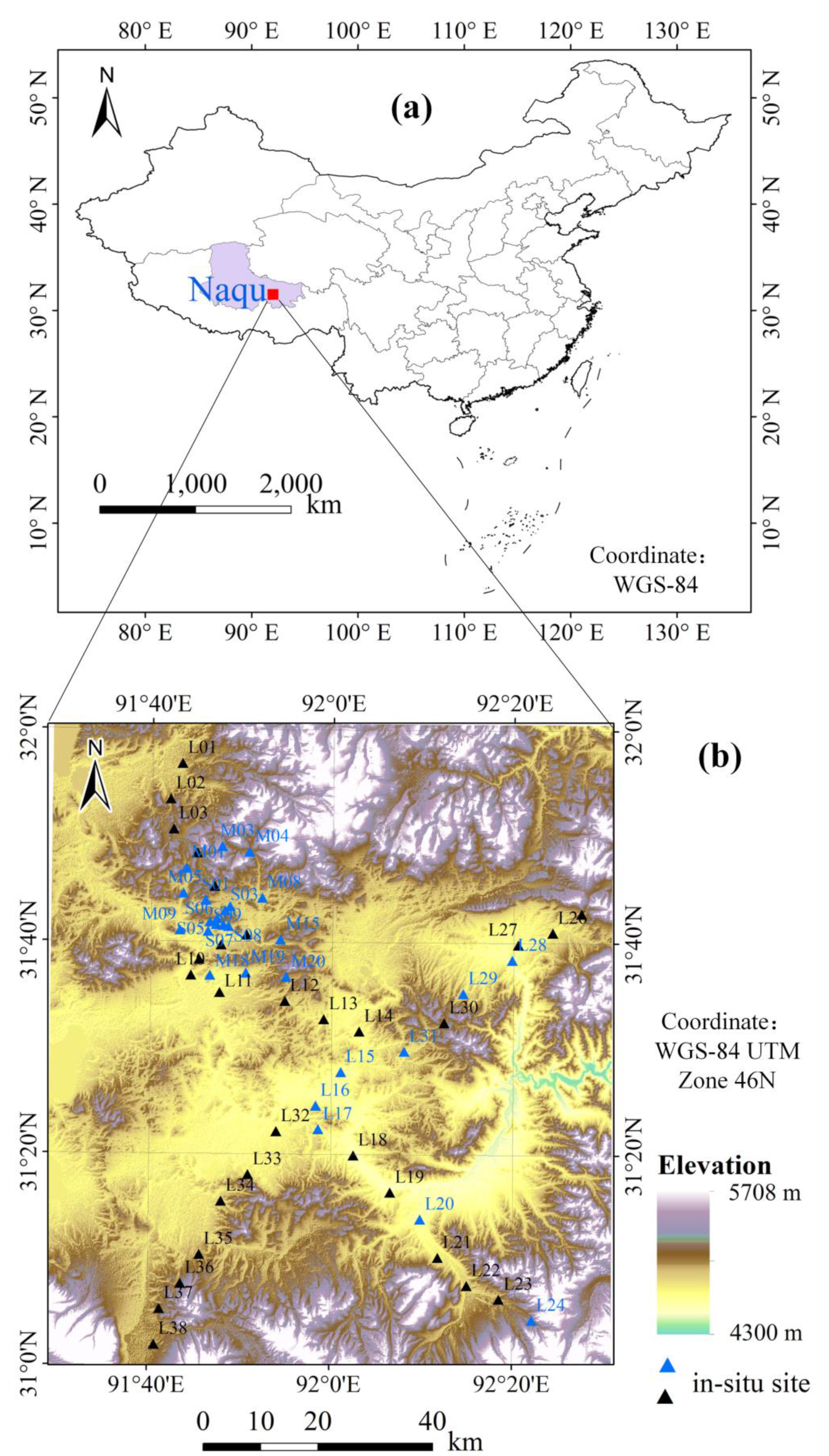
2.1.1. Study Area and In Situ Surface Soil Moisture Data

The study area is located in Naqu, central Tibet Plateau (Figure 1a). The in situ SSM data used are from the Soil Moisture and Temperature Monitoring Network (SMTMN) in Naqu, which is deployed by Yang et al. [37]. The SMTMN covers 1° × 1° geographical space (91.5° E–92.5° E, 31° N–32° N), which contains 57 in situ sites. The real time SSM of 0–5, 10, 20, and 40 cm is measured in volumetric water content using the EC-TM and 5TM monitoring equipment, which is manufactured by Decagon. The sensors measure SSM according to the sensitivity of soil dielectric permittivity to liquid soil water with an accuracy of 0.001 m3/m3. The SSM data is recorded every 30 min, and each record reflects the average of SSM over the past half-hour. A total of 48 SSM records are collected per day. The in situ data of SMTMN has been shared to the International Soil Moisture Network (https://ismn.geo.tuwien.ac.at/en/networks/?id=CTP_SMTMN, accessed on 15 September 2021), and the time range is from 2008 to 2016. The first layer (0–5 cm) of in situ data was selected in this study. Regarding soil texture of SMTMN, silt and sand are dominant components with a comparable magnitude, while clay content consistently maintains at a low level (less than 10%). The range of altitudes of in situ sites is 4450–5000 m and is grassland-dominated. The relatively homogeneous area is convenient for MODIS SSM retrieval. This area belongs to the sub-frigid climate zone. According to a previous study [38], the period from October to May is defined as the frozen period, as the land surface temperature (LST) is below 0 °C most of the time. Meanwhile, the other period of the year (June to September) is the unfrozen period. Soil freezing in frozen period has an adverse impact on SSM monitoring. To improve the reliability of the study, the proposed SMRFM is only implemented in unfrozen period.

2.1.2. Aqua AMSR-E Soil Moisture

The multi-frequency dual polarization AMSR-E sensor mounted on the Aqua satellite is developed by JAXA and can be used to monitor the changes of SSM [39,40]. The ascending and descending time of AMSR-E are 01:30 PM and 01:30 AM local time, respectively. The spatial resolution of SSM released by AMSR-E is ~25 km. The expected accuracy of AMSR-E is 0.06 m3/m3 in low-to-medium vegetation coverage areas [11]. A variety of products have been retrieved and released based on AMSR-E observations [41], the most notable of which are released by NASA and JAXA. The root mean square error (RMSE) of JAXA AMSR-E SSM (<0.12 m3/m3) is lower than NASA data (>0.16 m3/m3) in the study area shown in previous study [12]. Therefore, JAXA AMSR-E SSM is used for SSM downscaling in the study. For the sensor failure, AMSR-E could not continuously observe the Earth and release the SSM product after October 2011 [16]. It was officially retired after nearly ten years of in-orbit operation. The time range of SSM products released by AMSR-E data is from May 2002 to October 2011. The Shizuku satellite equipped with AMSR2 sensor was launched by JAXA for the replacement of AMSR-E in May 2012. It continues to carry out Earth observation and release global ~25 km SSM products [16]. To match the pixel size of MODIS data, AMSR-E data were resampled to 1 km using the cubic convolution interpolation method in ArcGIS software.

2.1.3. Aqua MODIS Optical and Thermal Infrared Data

MODIS sensors are carried on Terra and Aqua satellites. Aqua MODIS data is selected to reduce the adverse impact of AMSR-E and MODIS on observation time mismatch. The MYD11A1 daily 1 km LST data and the MYD13A1 8-day 500 m composited Normalized Difference Vegetation Index (NDVI) data are used to fit the empirical equation for MODIS SSM retrieval. Because of the composited product of MODIS NDVI, it assumes that the NDVI is constant in the 8-day composited date [42]. The LST gradients are normally reduced at nighttime, which is more beneficial to SSM retrieval [3]. Therefore, the Aqua MODIS LST at nighttime is used to eliminate the observation time difference between the two datasets for improved MODIS SSM retrieval. As the visible light cannot be used at nighttime, the Aqua MODIS NDVI data (visible light data) is used at daytime.

2.1.4. SRTM DEM Data

The SRTM digital elevation model (DEM) data, produced by NASA originally, are a major breakthrough in the digital mapping of the world. The 90 m SRTM DEM (version 4) used was downloaded from https://srtm.csi.cgiar.org/srtmdata/ (accessed on 12 October 2021) in this study. For more information about the used SRTM DEM, refer to [43]. After data mosaicking and clipping, the 90 m STRM DEM were resampled to 1 km pixel size using the cubic convolution interpolation method in ArcGIS software. As altitude (m) and slope (°) extracted from STRM DEM data play an important role in the redistribution of SSM, they were selected for MODIS SSM retrieval in the study.

2.1.5. Noah Land Surface Model L4 Central Asia Daily Soil Moisture

As OTI data are seriously polluted by clouds, it is difficult for traditional microwave SSM downscaling methods to effectively estimate MODIS SSM with long time series. Therefore, it is inappropriate to compare the SMRFM method proposed in the study with the traditional microwave SSM downscaling methods. Alternatively, the SSM data simulated by the land surface model were used as comparative data to verify the MODIS SSM with long time series estimated by SMRFM. The comparative data were acquired from the FLDAS Noah Land Surface Model L4 Central Asia Daily dataset (version 001) [44], which is simulated from the Noah 3.6.1 model in the Famine Early Warning Systems Network Land Data Assimilation System, adapted from Land Information System. This dataset contains a series of land surface parameters in a 0.01-degree spatial resolution over the Central Asia region (30–100° E, 21–56° N) from October 2000 to present. The four layers SSM data were comprised by the daily dataset and the top layer (0–10 cm) SSM in volumetric water content was used as the comparative dataset in the study. The 0.01-degree simulated SSM is resampled and then clipped to 1-km size for matching the pixel of fused MODIS SSM. In November 2020, all FLDAS Noah data were post-processed with the MOD44 MODIS land mask, so the simulated SSM data were missing over inland water in the study.
All data used in this study are shown in Table 1. As the temporal coverage of different data is different, the temporal intersection of AMSR-E and MODIS data in unfrozen period (1 August–31 September 2010 and 1 June–31 September 2011, six months in total) was used as the study period.

2.2. Methods

The MODIS SSM with long time series is estimated by downscaling AMSR-E SSM from coarse scale using proposed SMRFM. A reference MODIS SSM is retrieved from the coupling of in situ data, MODIS OTI data and topographic information. Then, the long time series AMSR-E SSM is downscaled to MODIS scale using the reference MODIS SSM and STFM. Therefore, SMRFM solves the difficulty of MODIS SSM acquisition in STFM and can be taken as an improvement for STFM in SSM.

2.2.1. Data Pre-Processing

The average daily in situ SSM is used for further analysis. As the in situ SSM is 0–0.6 m3/m3 in SMTMN [37,39], AMSR-E data higher than 0.6 m3/m3 is excluded in the study. In addition, the pre-processing manners of in situ data are different for different application scenarios in the study. For reference MODIS SSM retrieval and daily evaluation, the daily 57 in situ data (the triangle shown in Figure 1b) is used. For temporal evaluation, the in situ data is selected according to the following four conditions: (1) the data quality of in situ data should be marked “G” (Good); (2) the monitored surface soil depth should be less than 5 cm at first layer; (3) the temporal correlation between in situ SSM and the corresponding AMSR-E SSM should be positive and pass the hypothesis test (p-value is less than 0.05). After the selection, 29 in situ sites (the black triangle shown in Figure 1b) are used for temporal evaluation in the study.

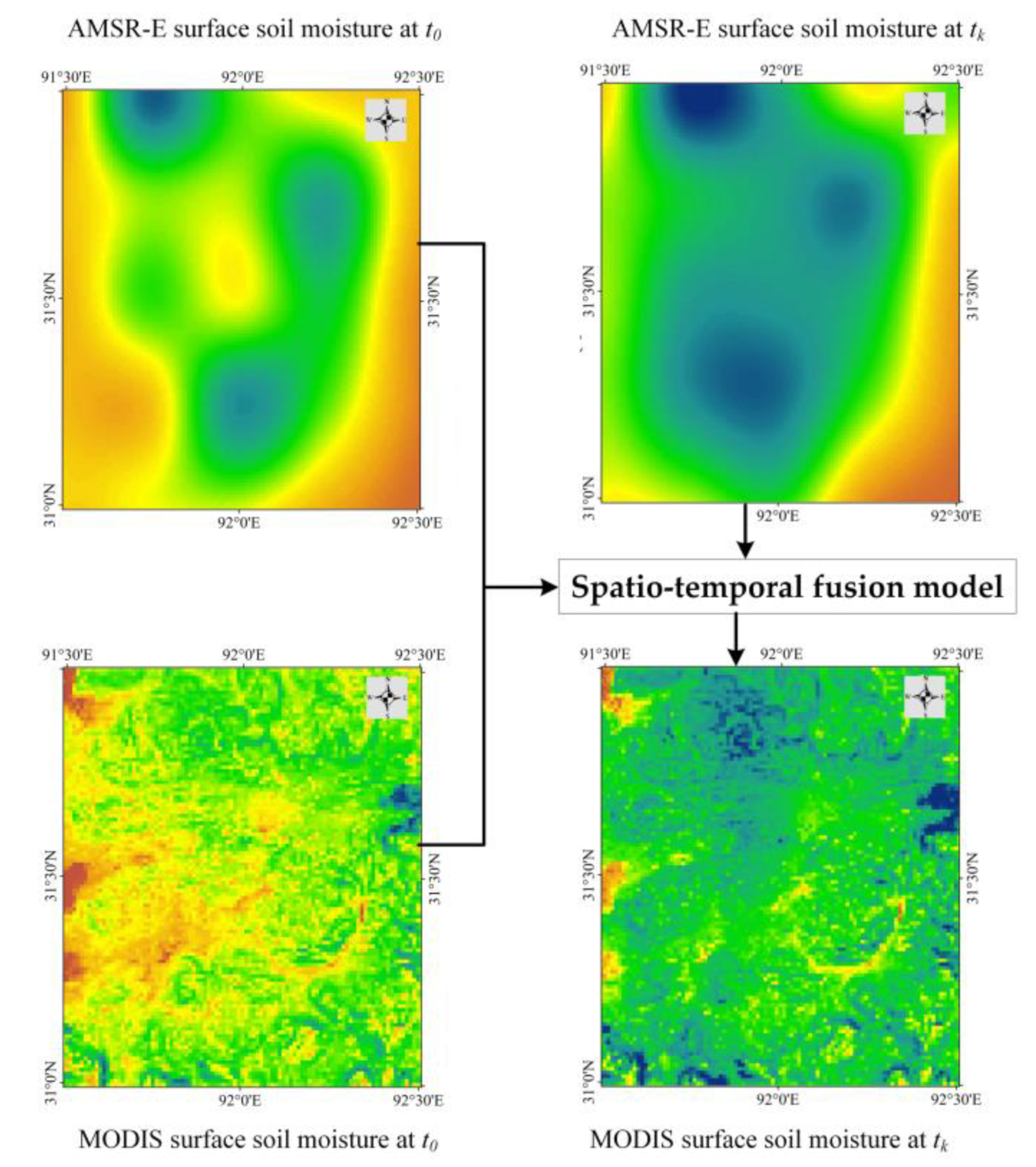
2.2.2. Spatio-Temporal Fusion Model

The SSM STFM (Figure 2) takes the known MODIS SSM and the corresponding AMSR-E SSM as the paired reference data at t 0 date and then again to fuse t k date AMSR-E SSM for the unknown MODIS SSM estimation at the date. Notably, the date of reference data is taken as the reference date. The estimation needs to excavate the spatio-temporal correlation characteristics between AMSR-E and MODIS SSM without the help of other additional remote sensing auxiliary data. In practice, one or more paired reference datasets can be used to estimate MODIS SSM at t k date. The more paired reference data that is used, the more restrictive the conditions of the model. As the main aim of the study is to verify the feasibility of the proposed SMRFM, only one paired reference dataset is used in the STFM.
From the reference date t 0 to the prediction date t k , temporal variation of SSM can be fitted by a linear equation. For AMSR-E SSM ( S S M M ), the linear equation is as follows:
S S M M t k = a x , y , Δ t × S S M M t 0 + b x , y , Δ t
where Δ t = t k t 0 ,  a and b are the regression coefficients of the linear equation that are calculated by the least-squares method. As the model assumes that SSM has the same temporal change at different scales [45], the regression coefficients estimated at AMSR-E scale can be applied to MODIS scale. Thus, the MODIS SSM at date t k can be estimated using Equation (2).
S S M F t k = a x , y , Δ t × S S M F t 0 + b x , y , Δ t
The change of SSM in each pixel may be different with the change of time. The fixed regression coefficients for the remotely sensed image may have a negative impact on prediction. To make the prediction result more accurate, the information of similar pixels in the neighborhood moving sliding window (e.g., 5 × 5) is used in the model. The prediction expression is as follows,
S S M F x w / 2 , y w / 2 , t k = i = 1 l W x i , y i , t 0 × a x , y , Δ t × S S M F t 0 + b x , y , Δ t
where w and w / 2 are the size and center of moving window, respectively, x i , y i indicates similar pixels, and l is the number of similar pixels. Thus, the regression coefficients of each pixel may be different for MODIS SSM estimation. For the selection of similar pixels and the calculation of linear regression coefficients in the fusion model, please refer to [33] for details.
From the above equations, it can be seen that the paired AMSR-E and MODIS SSM at reference date t 0 and the AMSR-E SSM at t k are used to predict the MODIS SSM at t k . In this process, there is no need to rely on other remote-sensing auxiliary data. However, the MODIS SSM at reference date t 0 is also unknown in most cases. Therefore, the Aqua MODIS LST and NDVI data are used for SSM retrieval in the study and then again to estimate the MODIS SSM at reference date t 0 .

2.2.3. Aqua MODIS Surface Soil Moisture Retrieval

OTI data cannot penetrate clouds, vegetation, and soil surface layers, and do not meet the conditions of the remote-sensing radiation transfer equation for SSM retrieval. Therefore, the SSM retrieval from OTI data lacks physical basis. In many cases, the use of OTI data to monitor SSM is mainly based on the correlation between SSM and remote-sensing surface parameters such as vegetation index, surface temperature [46], thermal inertia [47], surface reflectance [48], drought index [49,50]. Then, empirical equations between SSM and the remotely sensed surface parameters are established to retrieve regional SSM. The study develops a MODIS SSM retrieval model using in situ data, OTI data (LST and NDVI), altitude, and surface slope data which are calculated by the DEM data (Equation (4)).
S S M F = a 1 × L S T + a 2 × N D V I + a 3 × a l t i t u d e + a 4 × S l o p e + a 5
where a i   ( i = 1 , 2 , 3 , 4 , 5 ) are regression coefficients fitted by the least-squares method. To weaken the uncertainty caused by the spatial matching between the in situ SSM data and the remotely sensed pixel data, a 3 × 3 neighborhood average of the pixel corresponding to the in situ site location is taken as the matching value. Moreover, neighborhood average can weaken the information distortion that may exist in the single pixel value corresponding to the in situ site location. This can improve the robustness of MODIS SSM retrieval model (Equation (4)).
To estimate MODIS SSM using Equation (4), MODIS LST should meet the following two conditions: cloud-free and temperature higher than 0 °C (unfrozen soil). In general, the more training samples, the higher probability of the accuracy and stability of the fitting formula. To achieve this goal, the percentage of uncontaminated pixels in daily MODIS LST during the study period was calculated (Figure 3). This showed that the number of days for which the percentage of uncontaminated pixels is greater than 80% does not exceed 21 days. This suggests that number of days is relatively small for SSM estimation using Equation (4) in the study period. After careful screening, it was found that only 5 days of MODIS LST data were 100% uncontaminated. At the same time, the number of in situ sites for the days was counted. It was found that the number of effective in situ sites was the largest on 24 July 2011 among the 5 days, reaching as many as 48. Therefore, the MODIS SSM on 24 July 2011 is retrieved by Equation (4).
To avoid over-fitting of SSM retrieval equation (Equation (4)) using least-squares method, the 48-sample dataset (in situ data and its corresponding remote sensing data) on 24 July 2011 is sorted by in situ SSM in ascending order. Then, the dataset is divided into five subsets at an interval of five, and the second subset with a sample size of ten is taken as the validation dataset, and the remaining 38 samples are taken as the training dataset.
Theoretically, the average value of regional SSM should not change with the varied scale. AMSR-E SSM has a stronger theoretical basis than that of SSM retrieved from OTI data. Therefore, the regional SSM retrieved by microwave data should be better than that of OTI data in theory. To ensure the same regional average SSM between AMSR-E and MODIS SSM, the AMSR-E SSM is taken as the benchmark and is used to correct retrieved MODIS SSM using Equation (5).
S S M F C = S S M F a v e r a g e ( S S M F ) × a v e r a g e ( S S M M )
where SSMFC is the corrected MODIS SSM, average () is the average of SSM. The corrected MODIS SSM is taken as the reference SSM in the STFM.

2.2.4. Evaluation Methods

The correlation coefficient (r), RMSE, bias, and the unbiased RMSE (μbRMSE) are used as the indicators for accuracy evaluation.
r = i = 1 n ( S S M p i x e l , i S S M p i x e l ¯ ) × ( S S M r e f , i S S M r e f ¯ ) i = 1 n ( S S M p i x e l , i S S M p i x e l ¯ ) 2 × i = 1 n ( S S M r e f , i S S M r e f ¯ ) 2
R M S E = i = 1 n ( S S M p i x e l , i S S M r e f , i ) 2 n
b i a s = S S M p i x e l S S M r e f
μ b R M S E = R M S E 2 b i a s 2
where S S M p i x e l , i and S S M p i x e l ¯ are the pixel SSM and the average pixel SSM, and S S M r e f , i and S S M r e f ¯ are the reference SSM and the average reference SSM. The direct and indirect evaluations are implemented to evaluate the accuracy of pixel SSM and to investigate the feasibility of the proposed SMRFM for MODIS SSM estimation.
The in situ data are taken as the reference SSM and then again to directly compare the difference between the in situ SSM and the pixel SSM neglecting the spatial matching difference. This method is often used for accuracy evaluation of the satellite based SSM in previous studies [23,51,52]. The in situ sites for temporal evaluation (the black triangle shown in Figure 1b) are evenly distributed throughout the study area, and their average value can be considered as the SSM at SMTMN scale. Therefore, the fused MODIS SSM, AMSR-E SSM, and Noah SSM are evaluated against in situ SSM at SMTMN scale. It can be used to evaluate the overall temporal accuracy of pixel SSM. To demonstrate the individual difference of pixel SSM at each in situ site, the temporal accuracy of pixel SSM against in situ data is calculated at MODIS scale. Like the evaluation at SMTMN scale, the temporal variation of pixel SSM is used to directly compare in situ data. Instead of using overall average of all selected in situ data, the observed temporal SSM is used at each site. In addition, the daily evaluation of pixel SSM against in situ data is also explored at MODIS scale in the study, so as to display all daily accuracies in pixel SSM. In general, the focus of temporal variation accuracy evaluation and daily accuracy evaluation are different. The former focuses on depicting temporal variation of SSM, and the temporal characteristics are emphasized. Therefore, the evaluation index pays more attention to temporal r and μbRMSE. Meanwhile, the latter focuses on describing spatial variation of SSM, and the characteristics of absolute value change are emphasized. The evaluation index pays more attention to RMSE and bias. Therefore, it is more convincing to carry out the evaluations in view of temporal variation and absolute value of pixel SSM at SMTMN scale and MODIS scale.
In fact, there is a spatial matching error between in situ data and pixel SSM, although evaluations based on in situ data are widely used. To eliminate the uncertainty of spatial matching, the triple collocation (TC) method is used for further evaluation. The TC method was proposed by Stoffelen [53] and was used to evaluate wind and wave height observations in oceanography. It was later introduced into remote-sensing SSM observation error estimation. For example, TC method is used to evaluate the global errors for ASCAT, AMSR-E, and ERA reanalysis SSM [54], which has shown that TC method is robust and can generate objective error estimates. There are four assumptions of TC method for temporal r estimation in the case of unknown truth values [55]: (1) there is a linear correlation between the three kinds of SSM and the unknown truth SSM; (2) the error is stable and does not change with temporal variation; (3) the errors of the three kinds of SSM are independent of each other; (4) the errors of the three kinds of SSM are independent of unknown truth values. As fused MODIS SSM and AMSR-E SSM are related to each other, a triplet pattern of in situ, Noah, and remote sensing SSM is built for the TC evaluation in the study. Two kinds of TC triplets are constructed: in situ Noah-fused MODIS SSM (TC1) and in situ Noah-AMSR-E SSM (TC2), so as to compare the temporal accuracy difference of the three kinds of pixel SSM at MODIS scale.

3. Results

3.1. Accuracy Analysis of MODIS Surface Soil Moisture Retrieval

The training and validation accuracy of the equation fitting for the retrieval of MODIS SSM is shown in Table 2.
Table 2 shows that the fitted equation (Equation (4)) has a good robustness for the comparable accuracy of training and validation datasets. The RMSE is less than 0.09 m3/m3 and the r is higher than 0.65. This indicates that the fitted equation can estimate MODIS SSM well. Then, the fitted equation is applied to retrieve MODIS SSM on 24 July 2011 (Figure 4) in the study.
The spatial distribution of the AMSR-E and MODIS SSM is consistent as a whole, but there are still certain spatial and numerical differences between them (Figure 4). The range of AMSR-E is 0.132–0.548 m3/m3, with an average of 0.323 m3/m3. The range of retrieved MODIS SSM is 0.036–0.690 m3/m3, with an average of 0.365 m3/m3. The coefficient of variation for AMSR-E is 0.259, and for retrieved MODIS SSM is 0.189. This suggests that the AMSR-E is more discrete than the retrieved MODIS SSM.
The average values of the AMSR-E and MODIS SSM are different, which is consistent with our expectation. Thus, the corrected SSM is calculated using Equation (5). The spatial distribution of the corrected MODIS SSM (Figure 4c) has not changed obviously when compared to Figure 4b in visual representation. However, the spatial fitness between AMSR-E and MODIS SSM is slightly improved. RMSE between them has decreased from 0.112 m3/m3 to 0.099 m3/m3 after correction. Therefore, the corrected MODIS SSM (Figure 4c) and AMSR-E SSM (Figure 4a) are used to construct the paired reference datasets of STFM in the study.

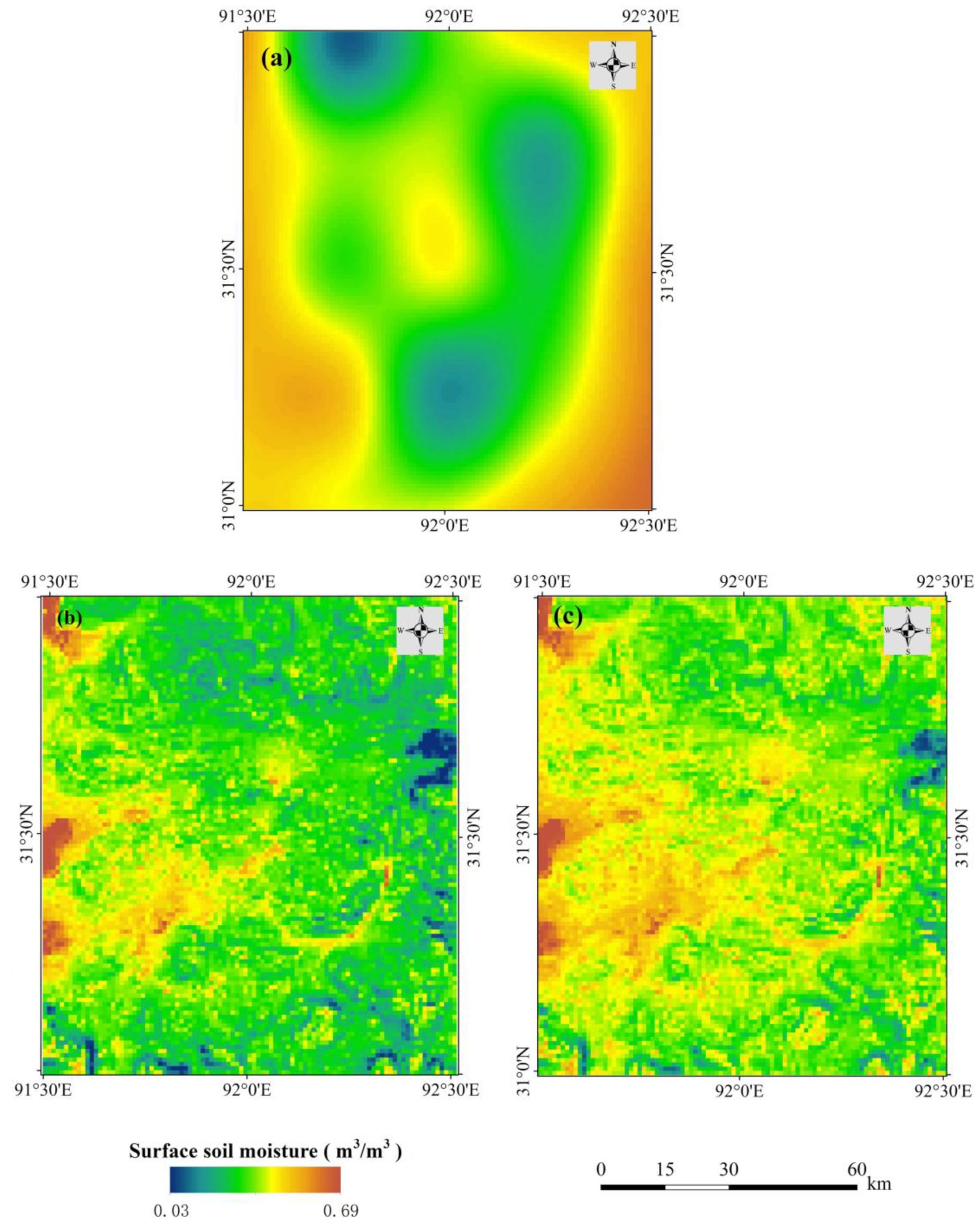
3.2. Fused MODIS Surface Soil Moisture

The long time series MODIS SSM is fused by SMRFM using one fixed paired reference dataset and the corresponding AMSR-E SSM at the unfrozen period. To validate the spatial downscaling ability of SMRFM, the spatial distribution of fused MODIS SSM at different dates is shown in Figure 5.
More detailed spatial information is presented in the fused MODIS SSM. It suggests that the SMRFM can improve the spatial resolution of AMSR-E SSM from microwave scale to MODIS scale well. The enhanced spatial information of fused MODIS SSM will be beneficial for applications at the regional scale. Meanwhile, the AMSR-E and fused MODIS SSM have relatively good consistency in the spatial distribution, indicating that the STFM can downscale AMSR-E SSM to fine scale from coarse scale well under large spatial resolution differences. For the large difference in spatial resolution of the two kinds of SSM (the paired reference data), there may be some inconsistencies in the fused results. It is mainly that the spatial variation of MODIS SSM in special areas cannot be well represented in AMSR-E SSM.
There are many spatial void data for Noah SSM, as they are masked by the land surface data, and the other two kinds of SSM are not masked. However, this does not affect the presentation of the results. In addition, the spatial distributions of AMSR-E and fused MODIS SSM are quite different when compared to Noah SSM. Nevertheless, the variation characteristics in temporal are still captured by the three kinds of SSM, but each SSM has some deviation in its depiction. This suggests the three kinds of SSM all have certain uncertainty, consistent with previous studies on satellite-based SSM [10,15,16].

3.3. Evaluations against In Situ Data at SMTMN Scale

The fused MODIS SSM, AMSR-E SSM, Noah SSM, and in situ SSM are aggregated to the SMTMN scale. Then the in situ site-based temporal variation differences between the three kinds of pixel SSM are compared (Figure 6). It shows that the pixel SSM can well monitor the temporal variations of regional SSM and display a good consistency in unfrozen period compared to in situ data. Nevertheless, the temporal variation of the four kinds of SSM differs greatly. The range of in situ data is 0.182–0.403 m3/m3, AMSR-E SSM is 0.106–0.601 m3/m3, fused MODIS SSM is 0.152–0.557 m3/m3 and Noah SSM is 0.238–0.455 m3/m3 at SMTMN scale. The ability of the fused MODIS SSM to capture in situ data is between AMSR-E and Noah SSM. As the fused MODIS SSM is downscaled by AMSR-E, there is high consistency in temporal variation curves.
The quantitative evaluation results (Table 3) show that the fused MODIS SSM is slightly higher than AMSR-E SSM and obviously higher than Noah SSM in terms of temporal r (0.673). Meanwhile, it presents lower temporal μbRMSE (0.070 m3/m3) than AMSR-E SSM against in situ data. Noah data present the lowest μbRMSE, however, it also gets the lowest temporal r. As the highest temporal r and the moderate temporal μbRMSE of fused SSM, it shows that the fused data have more advantages than the other pixel data against in situ data. Compared to improving the temporal r of AMSR-E, the fused MODIS SSM has more advantages in decreasing the temporal RMSE of AMSR-E. This suggests that the fused SSM has higher accuracy than AMSR-E SSM in overall temporal variation at SMTMN scale.

3.4. Evaluations against In Situ Soil Moisture at MODIS Scale

In terms of overall temporal accuracy at SMTMN scale, it can be considered that the fused MODIS SSM outperforms AMSR-E in describing temporal variation of in situ data. However, the accuracy difference between the pixel SSM is still unclear at the MODIS scale and needs to be further explored.

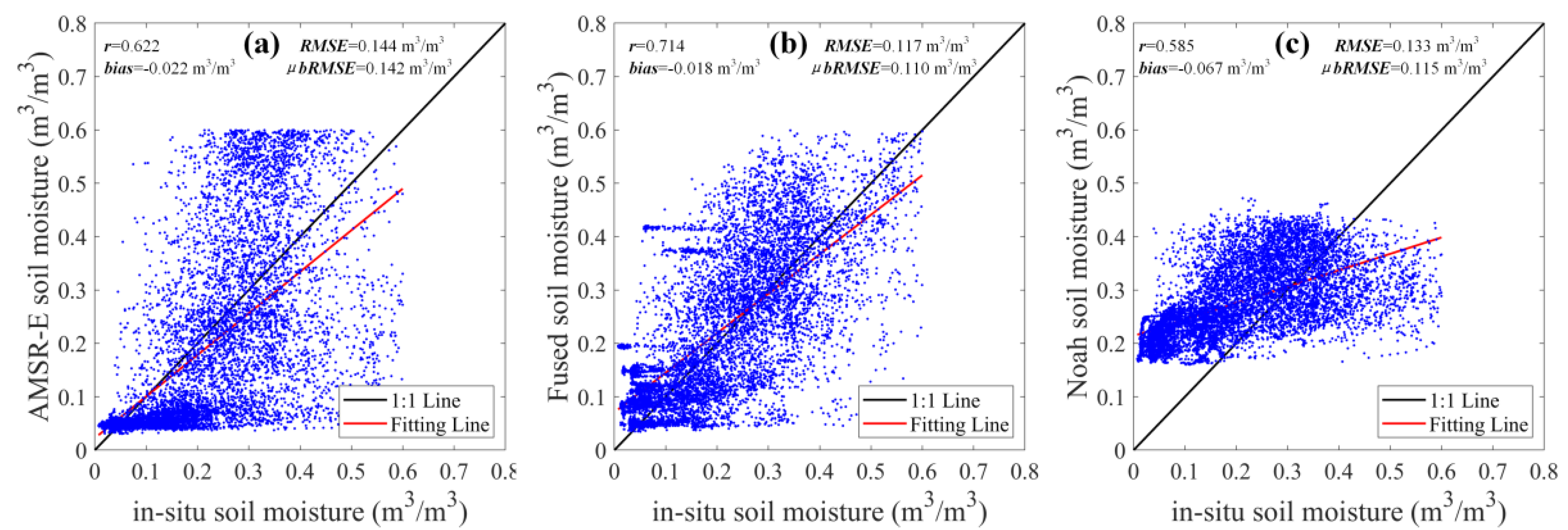
3.4.1. Daily Accuracy Evaluation

To calculate the daily evaluation of pixel SSM against in situ data effectively, all the available daily pixel SSM and in situ SSM are collected at MODIS scale during unfrozen period. The scatter plots between them are shown in Figure 7. It shows that the fitting line of the scatter between in situ and fused MODIS SSM is closest to the 1:1 line. Noah and in situ SSM present the lowest slope of fitting line. Among quantitative indexes, fused MODIS SSM presents the highest r (0.714) and the lowest RMSE (0.117 m3/m3) compared to AMSR-E and Noah SSM. It reveals that the fused MODIS SSM gets the best evaluation indexes at the MODIS scale indicating the advantages of SMRFM.

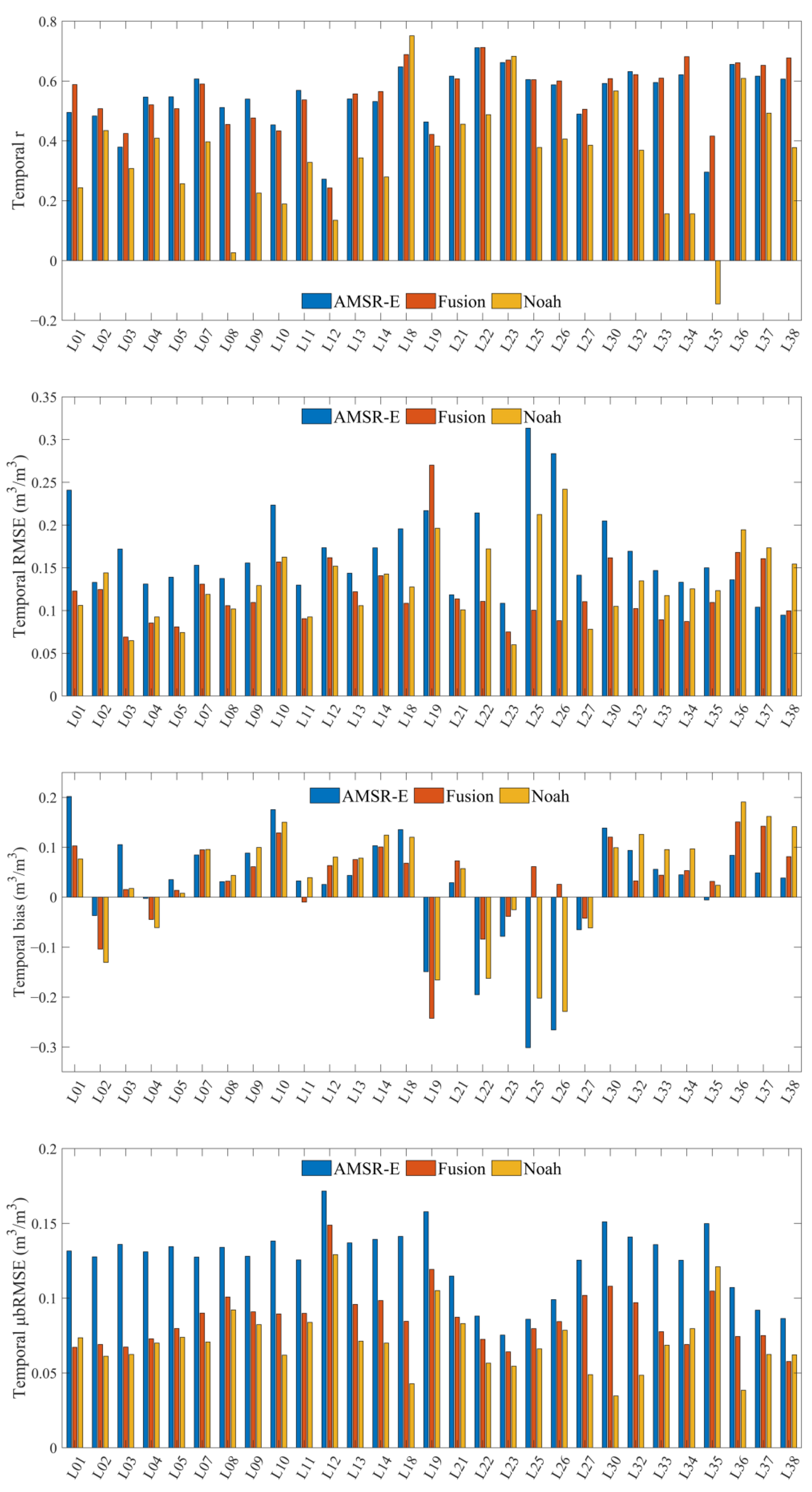
3.4.2. Temporal Accuracy Evaluation

To further demonstrate the difference between the three kinds of pixel SSM, the temporal accuracy is investigated at MODIS scale. The fused MODIS SSM, AMSR-E SSM, and Noah SSM are extracted based on the selected 29 in situ sites. Then they are directly temporal evaluated against the in situ data. The evaluation results at the 29 in situ sites were obtained in the study (Figure 8), and the average values are shown in Table 4.
In terms of temporal r, the range of fused MODIS SSM is 0.243–0.722 with an average of 0.557, the range of AMSR-E SSM is 0.275–0.728 with an average of 0.547, and the range of Noah SSM is −0.143–0.759 with an average of 0.348. For temporal RMSE, the range of fused MODIS SSM is 0.073–0.276 m3/m3 with an average of 0.119 m3/m3, the range of AMSR-E SSM is 0.097–0.314 m3/m3 with an average of 0.167 m3/m3, and the temporal RMSE range of Noah SSM is 0.067–0.248 m3/m3 with an average of 0.131 m3/m3. For temporal bias, the range of fused MODIS SSM is −0.243–0.151 m3/m3 with an average of 0.035 m3/m3, the range of AMSR-E SSM is −0.301–0.204 m3/m3 with an average of 0.017 m3/m3, and the range of Noah SSM is −0.237–0.191 m3/m3 with an average of 0.031 m3/m3. For temporal μbRMSE, the range of fused MODIS SSM is 0.053–0.152 m3/m3 with an average of 0.087 m3/m3, the range of AMSR-E SSM is 0.074–0.176 m3/m3 with an average of 0.126 m3/m3, and the range of Noah SSM is 0.037 −0.134 with an average of 0.071 m3/m3.
In most cases, the temporal r of Noah SSM is lower than AMSR-E and fused SSM (Figure 8). The negative correlation of Noah SSM at L35 site indicates that it could not describe the temporal variation of in situ data well. The temporal r of fused MODIS SSM is higher than AMSR-E at 17 in situ sites. The temporal bias is positive at most sites, indicating that the pixel SSM overestimates the in situ data. For temporal RMSE and μbRMSE, the similar change characteristics are displayed. The higher RMSE and μbRMSE are obtained by AMSR-E at each site. Meanwhile, the difference between fused MODIS SSM and Noah SSM is not very large in the temporal RMSE and μbRMSE at each site.
Compared to the temporal evaluation at SMTMN scale, the fused SSM presents better evaluation indexes than the AMSR-E in terms of temporal r, RMSE and μbRMSE (Table 3 and Table 4). Meanwhile, Noah SSM presents the lowest average temporal r and temporal μbRMSE at MODIS scale, which is consistent with the temporal evaluation at SMTMN scale. Notably, the temporal r of five sites failed the hypothesis test (p-value > 0.05) for Noah SSM.

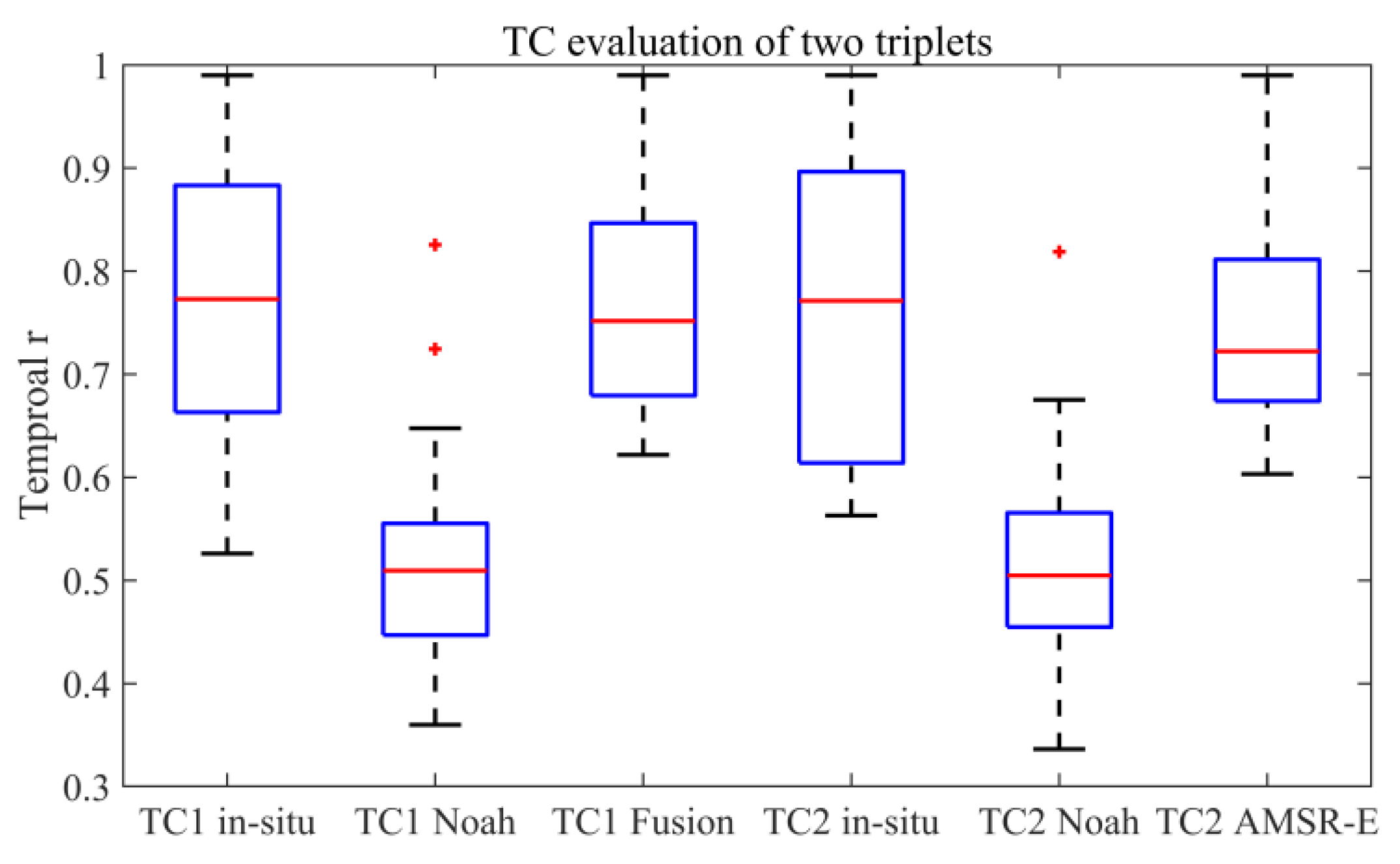
3.5. Evaluations Based on Triple Collocation Method

Referring to previous studies [45,55], the valid number of data points should be greater than 100 for each pixel SSM in the TC triplet. Like the temporal evaluation against in situ data, the TC evaluations are still carried out at the selected 29 in situ sites (the black triangle shown in Figure 1b). The boxplot of TC1 (in situ Noah-Fusion TC triplet) and TC2 (in situ Noah-AMSR-E TC triplet) evaluations is shown in Figure 9.
The average temporal r of in situ SSM is the best in each TC triplet. The ranges of temporal r for in situ data, Noah SSM, and fused SSM are 0.526–0.990, 0.361–0.837, and 0.623–0.991, with averages of 0.762, 0.521, and 0.761 in TC1. Meanwhile, the ranges of temporal r for in situ data, Noah SSM, and AMSR-E SSM are 0.563–0.990, 0.348–0.826, and 0.602–0.991, with averages of 0.766, 0.518, and 0.755 in TC2. The average temporal r of in situ data is comparable in each TC triplet, as is the Noah SSM. Thus, direct comparison can be implemented between the TC temporal r of AMSR-E and the fused MODIS SSM. Therefore, the average temporal r of the four kinds of SSM can be sorted as follows: in situ SSM > the fused MODIS SSM > AMSR-E SSM > Noah SSM. This suggests that the proposed SMRFM can be used to estimate fine-scale SSM with long time series and that the estimated SSM is better than the AMSR-E SSM in temporal variation evaluated by TC method at MODIS scale in the study.

4. Discussion

The SMRFM is proposed to downscale AMSR-E SSM to MODIS scale with long time series in this study. To evaluate the accuracy of estimated MODIS SSM, the r, RMSE, bias, and μbRMSE are used in the study. A higher r indicates a higher explained variability and a lower RMSE indicates a higher agreement between the pixel SSM and in situ data in absolute value. Positive bias indicates that the in situ data are overestimated by pixel SSM. The lower μbRMSE indicates a higher agreement between the pixel SSM and in situ data in relative value. Therefore, the high accuracy of pixel SSM indicates the high r, the low RMSE, and μbRMSE.
For the spatial mismatch between pixel and in situ SSM, the direct comparison between them has always been controversial [3,7,9]. To evaluate the pixel SSM better using in situ data, the upscaling methods are developed and used in the previous studies [47,56]. Nevertheless, the direct comparison is still the most basic evaluation for pixel SSM, as the in situ data are first-hand real data and can more directly express the changes of actual SSM. Moreover, the effect of spatial mismatch on absolute value comparison of SSM is higher than that of temporal variation [45]. More importantly, the TC method is used for SSM evaluation under the unknown true data. There are two TC triples for evaluations in the study. Both of them show that the in situ data present the highest temporal r (Figure 9). Therefore, it is reasonable to evaluate the pixel SSM using the in situ data in temporal variation. As there is only one in situ site in each MODIS pixel, the daily accuracy evaluations in Section 3.4.1 may be a compromise way to evaluate the absolute SSM in the case of absent true pixel SSM.
There are two keys for MODIS SSM estimation using proposed SMRFM. One is the OTI-data-based fine-scale SSM retrieval, another is the STFM. The training and validation accuracies of Equation (4) are comparable in the study. The RMSE of retrieved fine-scale SSM was less than 0.09 m3/m3 on 24 July 2011. Meanwhile, the RMSE of AMSR-E and Noah were 0.128 m3/m3 and 0.122 m3/m3 against in situ data on that day. The RMSE of AMSR-E is no less than 0.11 m3/m3 [39] and the downscaled AMSR-E [39] and SMAP SSM [24] is no less than 0.08 m3/m3 at Naqu, central Tibet Plateau. It can be concluded that the RMSE of retrieved OTI-based SSM is better than the AMSR-E SSM and is comparable with the downscaled SSM. The slope and altitude information of topographic attributes are used to fit the Equation (4). The impact of topographic changes on soil moisture may not be fully considered in the study. Therefore, the index characterizing the information of topographic wetness [57] for OTI-data-based SSM retrieval will be explored in future research.
The fused MODIS SSM significantly improves the spatial detailed information of AMSR-E SSM. Meanwhile, the evaluation indexes of fused data are better than AMSR-E SSM at SMTMN and MODIS scale. There may be several reasons for this result. The key reason may be that the neighborhood information is used by SMRFM for fine-scale SSM estimation. This is equivalent to denoising remote-sensing images using spatial filtering methods [33], which weakens the outliers in temporal variation of SSM. Thus, the temporal variation of estimated data is much smoother than the AMSR-E SSM (Figure 6). The reference MODIS SSM of SMRFM is estimated by Equation (4), which is fitted by the MODIS OTI data, in situ SSM, and the topographic information. Then, the SMRFM is used to estimate MODIS SSM with long time series using the fixed reference data. Therefore, the estimated MODIS SSM by SMRFM can be considered as coupled with the in situ SSM information. This may be another reason for the high accuracy of fused MODIS SSM. According to the basic principles of STFM [26,33], the smaller the difference in temporal variation, the better that MODIS SSM can be estimated [45]. The dominate land cover type of the study area is grassland, and the implementation of SMRFM should not exceed one-and-a-half years. This indicates that the spatial and temporal pattern of SSM will not change much in a relatively long time under the homogeneous land type. This may be a possible factor in the high accuracy of fused MODIS SSM.
There is an assumption that the temporal change is scale-invariant in STFM. The assumption was proposed in 2006 for surface reflectance estimation [26] and was then applied for other surface parameters estimation [27,28,29,30,31,32]. It is used as a downscaling method for long time series MODIS SSM estimation in the study. Similar with STFM, the scale-invariant assumption also exists in traditional microwave SSM downscaling, but it refers to scale-invariance of the relation between microwave SSM and other remotely sensed parameters for traditional methods in most cases [22,24]. It has been shown that the downscaling capability of STFM is better than that of the traditional downscaling method [45], although the scale-invariant assumption of temporal change is fitted by a linear equation. This may reveal that the scale-invariant assumption in temporal change is more reasonable than scale-invariance in the relation.
To investigate the relation between surface parameters and SSM, the correlations between LST, NDVI, altitude, and slope are calculated in Table 5. It shows that the correlations between SSM and the first two factors (LST and NDVI) are obviously better than the last two (altitude and slope). The correlation of the factors can be sorted as follows: NDVI > LST > Slope > Altitude. This suggests that the topographic factors may be limited in SSM estimation in this study.
Since MODIS SSM is downscaled from AMSR-E data using SMRFM, they have the same temporal resolution. Nevertheless, the effectiveness of proposed SMRFM in estimating SSM in highly heterogeneous areas and longer time series needs to be further explored. Notably, the premise of SMRFM for SSM estimation is to estimate the reference SSM. In the study, the OTI data are used for reference SSM retrieval. As OTI data cannot penetrate the surface, the use of Sentinel-1 and OTI data in SMRFM framework may enhance the accuracy and spatial resolution of estimated SSM. Therefore, the SMRFM has the potential to estimate long time series finer-scale (less than 1 km) SSM with the finer-scale reference SSM provides.

5. Conclusions

Given the difficulty of taking into account the long time series characteristics of current downscaling method, which integrates microwave SSM data and OTI data to estimate fine scale SSM, an SSM retrieval-and-fusion model named SMRFM is proposed to downscale AMSR-E SSM for MODIS SSM with long time series estimation in the study. The method was applied to the SMTMN over Naqu, central Tibet Plateau to obtain the MODIS SSM with long time series characteristics of microwave data. To validate the SMRFM, in situ data and Noah land surface model 0.01-degree SSM were used in the study. The main conclusions of the study are as follows:
(1)
A method that integrates in situ data, remote sensing OTI data, and terrain data was developed for MODIS SSM retrieval, and the estimated MODIS SSM by this method obtains an RMSE of less than 0.09 m3/m3.
(2)
The MODIS SSM fused by the SMRFM can well maintain the spatial distribution and temporal variation of AMSR-E data, although there are certain differences in the special distinction between the two kinds of pixel SSM.
(3)
Six months of MODIS SSM in unfrozen period were fused by the proposed SMRFM. The evaluations show that the fused MODIS SSM has better temporal accuracy than that of AMSR-E at SMTMN and MODIS scale. Compared to Noah SSM, the fused SSM presents higher temporal r and slightly lower μbRMSE. In addition, the fused SSM has better daily accuracy than AMSR-E and Noah SSM. Therefore, it can be considered that the proposed SMRFM can be used to estimate fine-scale SSM with long time series and that the estimated SSM is better than AMSR-E SSM in temporal variation. This will promote the development of research and applications with long time series SSM at regional scale.

Author Contributions

Conceptualization, H.J. and S.C.; methodology, H.J. and J.W.; software, J.W.; validation, H.J., J.Z. and L.W.; formal analysis, X.L.; investigation, J.W.; resources, S.C.; data curation, H.J.; writing—original draft preparation, H.J.; writing—review and editing, S.C., X.L. and J.W. All authors have read and agreed to the published version of the manuscript.

Funding

This research was funded by the National Natural Science Foundation of China (Grand no. 42101401), Guangdong Provincial Water Conservancy Science and Technology Innovation Project (Grand no. 2020-30), Scientific research project of Zhongkai University of Agriculture and Engineering (Grand no. KA22016B770).

Data Availability Statement

The study was performed based on public access remote sensing and in situ data. The fused MODIS surface soil moisture with long time series that support the findings of the study are available from the corresponding author and first author upon reasonable request.

Acknowledgments

We would like to thank JAXA for making the AMSR-E soil moisture data publicly available and ISMN for providing the SMTMN in situ soil moisture data. We would also like to thank the anonymous reviewers for their insightful comments on the manuscript.

Conflicts of Interest

The authors declare no conflict of interest.

References

  1. Sharma, K.; Irmak, S.; Kukal, M.S. Propagation of soil moisture sensing uncertainty into estimation of total soil water, evapotranspiration and irrigation decision-making. Agric. Water Manag. 2021, 243, 106454. [Google Scholar] [CrossRef]
  2. Babaeian, E.; Sadeghi, M.; Jones, S.B.; Montzka, C.; Vereecken, H.; Tuller, M. Ground, Proximal, and Satellite Remote Sensing of Soil Moisture. Rev. Geophys. 2019, 57, 530–616. [Google Scholar] [CrossRef] [Green Version]
  3. Dorigo, W.A.; Gruber, A.; De Jeu, R.A.M.; Wagner, W.; Stacke, T.; Loew, A.; Albergel, C.; Brocca, L.; Chung, D.; Parinussa, R.M.; et al. Evaluation of the ESA CCI soil moisture product using ground-based observations. Remote Sens. Environ. 2015, 162, 380–395. [Google Scholar] [CrossRef]
  4. Jadidoleslam, N.; Mantilla, R.; Krajewski, W.F.; Goska, R. Investigating the role of antecedent SMAP satellite soil moisture, radar rainfall and MODIS vegetation on runoff production in an agricultural region. J. Hydrol. 2019, 579, 124210. [Google Scholar] [CrossRef] [Green Version]
  5. Yoon, J.; Leung, L.R. Assessing the relative influence of surface soil moisture and ENSO SST on precipitation predictability over the contiguous United States. Geophys. Res. Lett. 2015, 42, 5005–5013. [Google Scholar] [CrossRef]
  6. Sabaghy, S.; Walker, J.P.; Renzullo, L.J.; Jackson, T.J. Spatially enhanced passive microwave derived soil moisture: Capabilities and opportunities. Remote Sens. Environ. 2018, 209, 551–580. [Google Scholar] [CrossRef]
  7. Wigneron, J.P.; Jackson, T.J.; O’Neill, P.; De Lannoy, G.; de Rosnay, P.; Walker, J.P.; Ferrazzoli, P.; Mironov, V.; Bircher, S.; Grant, J.P.; et al. Modelling the passive microwave signature from land surfaces: A review of recent results and application to the L-band SMOS & SMAP soil moisture retrieval algorithms. Remote Sens. Environ. 2017, 192, 238–262. [Google Scholar] [CrossRef]
  8. Karthikeyan, L.; Pan, M.; Wanders, N.; Kumar, D.N.; Wood, E.F. Four decades of microwave satellite soil moisture observations: Part 1. A review of retrieval algorithms. Adv. Water Resour. 2017, 109, 106–120. [Google Scholar] [CrossRef]
  9. Chan, S.K.; Bindlish, R.; O’Neill, P.E.; Njoku, E.; Jackson, T.; Colliander, A.; Chen, F.; Burgin, M.; Dunbar, S.; Piepmeier, J.; et al. Assessment of the SMAP Passive Soil Moisture Product. IEEE Trans. Geosci. Remote Sens. 2016, 54, 4994–5007. [Google Scholar] [CrossRef]
  10. Das, N.N.; Entekhabi, D.; Dunbar, R.S.; Chaubell, M.J.; Colliander, A.; Yueh, S.; Jagdhuber, T.; Chen, F.; Crow, W.; O’Neill, P.E.; et al. The SMAP and Copernicus Sentinel 1A/B microwave active-passive high resolution surface soil moisture product. Remote Sens. Environ. 2019, 233, 111380. [Google Scholar] [CrossRef]
  11. Njoku, E.G.; Jackson, T.J.; Lakshmi, V.; Chan, T.K.; Nghiem, S.V. Soil moisture retrieval from AMSR-E. IEEE Trans. Geosci. Remote Sens. 2003, 41, 215–229. [Google Scholar] [CrossRef]
  12. Zeng, J.; Li, Z.; Chen, Q.; Bi, H.; Qiu, J.; Zou, P. Evaluation of remotely sensed and reanalysis soil moisture products over the Tibetan Plateau using in-situ observations. Remote Sens. Environ. 2015, 163, 91–110. [Google Scholar] [CrossRef]
  13. Kerr, Y.H.; Waldteufel, P.; Richaume, P.; Wigneron, J.P.; Ferrazzoli, P.; Mahmoodi, A.; Al Bitar, A.; Cabot, F.; Gruhier, C.; Juglea, S.E.; et al. The SMOS Soil Moisture Retrieval Algorithm. IEEE Trans. Geosci. Remote Sens. 2012, 50, 1384–1403. [Google Scholar] [CrossRef]
  14. Jamei, M.; Mousavi Baygi, M.; Oskouei, E.A.; Lopez-Baeza, E. Validation of the SMOS Level 1C Brightness Temperature and Level 2 Soil Moisture Data over the West and Southwest of Iran. Remote Sens. 2020, 12, 2819. [Google Scholar] [CrossRef]
  15. Wang, Y.; Leng, P.; Peng, J.; Marzahn, P.; Ludwig, R. Global assessments of two blended microwave soil moisture products CCI and SMOPS with in-situ measurements and reanalysis data. Int. J. Appl. Earth Obs. 2021, 94, 102234. [Google Scholar] [CrossRef]
  16. Kim, S.; Liu, Y.Y.; Johnson, F.M.; Parinussa, R.M.; Sharma, A. A global comparison of alternate AMSR2 soil moisture products: Why do they differ? Remote Sens. Environ. 2015, 161, 43–62. [Google Scholar] [CrossRef]
  17. Liu, Y.; Zhou, Y.; Lu, N.; Tang, R.; Liu, N.; Li, Y.; Yang, J.; Jing, W.; Zhou, C. Comprehensive assessment of Fengyun-3 satellites derived soil moisture with in-situ measurements across the globe. J. Hydrol. 2021, 594, 125949. [Google Scholar] [CrossRef]
  18. Song, C.; Jia, L. A Method for Downscaling FengYun-3B Soil Moisture Based on Apparent Thermal Inertia. Remote Sens. 2016, 8, 703. [Google Scholar] [CrossRef] [Green Version]
  19. Merlin, O.; Walker, J.; Chehbouni, A.; Kerr, Y. Towards deterministic downscaling of SMOS soil moisture using MODIS derived soil evaporative efficiency. Remote Sens. Environ. 2008, 112, 3935–3946. [Google Scholar] [CrossRef] [Green Version]
  20. Peng, J.; Loew, A.; Merlin, O.; Verhoest, N.E.C. A review of spatial downscaling of satellite remotely sensed soil moisture. Rev. Geophys. 2017, 55, 341–366. [Google Scholar] [CrossRef]
  21. Piles, M.; Sanchez, N.; Vall-llossera, M.; Camps, A.; Martinez-Fernandez, J.; Martinez, J.; Gonzalez-Gambau, V. A Downscaling Approach for SMOS Land Observations: Evaluation of High-Resolution Soil Moisture Maps over the Iberian Peninsula. IEEE J. Sel. Top. Appl. Earth Obs. Remote Sens. 2014, 7, 3845–3857. [Google Scholar] [CrossRef] [Green Version]
  22. Senanayake, I.P.; Yeo, I.Y.; Willgoose, G.R.; Hancock, G.R. Disaggregating satellite soil moisture products based on soil thermal inertia: A comparison of a downscaling model built at two spatial scales. J. Hydrol. 2021, 594, 125894. [Google Scholar] [CrossRef]
  23. Wei, Z.; Meng, Y.; Zhang, W.; Peng, J.; Meng, L. Downscaling SMAP soil moisture estimation with gradient boosting decision tree regression over the Tibetan Plateau. Remote Sens. Environ. 2019, 225, 30–44. [Google Scholar] [CrossRef]
  24. Nasta, P.; Penna, D.; Brocca, L.; Zuecco, G.; Romano, N. Downscaling near-surface soil moisture from field to plot scale: A comparative analysis under different environmental conditions. J. Hydrol. 2018, 557, 97–108. [Google Scholar] [CrossRef] [Green Version]
  25. Li, Z.; Shen, H.; Li, H.; Xia, G.; Gamba, P.; Zhang, L. Multi-feature combined cloud and cloud shadow detection in GaoFen-1 wide field of view imagery. Remote Sens. Environ. 2017, 191, 342–358. [Google Scholar] [CrossRef] [Green Version]
  26. Gao, F.; Masek, J.; Schwaller, M.; Hall, F. On the blending of the Landsat and MODIS surface reflectance: Predicting daily Landsat surface reflectance. IEEE Trans. Geosci. Remote Sens. 2006, 44, 2207–2218. [Google Scholar] [CrossRef]
  27. Park, S.; Jeong, S.; Park, Y.; Kim, S.; Lee, D.; Mo, Y.; Jang, D.; Park, K. Phenological Analysis of Sub-Alpine Forest on Jeju Island, South Korea, Using Data Fusion of Landsat and MODIS Products. Forests 2021, 12, 286. [Google Scholar] [CrossRef]
  28. Meng, J.; Du, X.; Wu, B. Generation of high spatial and temporal resolution NDVI and its application in crop biomass estimation. Int. J. Digit. Earth 2013, 6, 203–218. [Google Scholar] [CrossRef]
  29. Shen, H.; Huang, L.; Zhang, L.; Wu, P.; Zeng, C. Long-term and fine-scale satellite monitoring of the urban heat island effect by the fusion of multi-temporal and multi-sensor remote sensed data: A 26-year case study of the city of Wuhan in China. Remote Sens. Environ. 2016, 172, 109–125. [Google Scholar] [CrossRef]
  30. Weng, Q.; Fu, P.; Gao, F. Generating daily land surface temperature at Landsat resolution by fusing Landsat and MODIS data. Remote Sens. Environ. 2014, 145, 55–67. [Google Scholar] [CrossRef]
  31. Qiu, Y.; Zhou, J.; Chen, J.; Chen, X. Spatiotemporal fusion method to simultaneously generate full-length normalized difference vegetation index time series (SSFIT). Int. J. Appl. Earth Obs. 2021, 100, 102333. [Google Scholar] [CrossRef]
  32. Zhao, W.; Duan, S. Reconstruction of daytime land surface temperatures under cloud-covered conditions using integrated MODIS/Terra land products and MSG geostationary satellite data. Remote Sens. Environ. 2020, 247, 111931. [Google Scholar] [CrossRef]
  33. Cheng, Q.; Liu, H.; Shen, H.; Wu, P.; Zhang, L. A Spatial and Temporal Nonlocal Filter-Based Data Fusion Method. IEEE Trans. Geosci. Remote Sens. 2017, 55, 4476–4488. [Google Scholar] [CrossRef] [Green Version]
  34. Emelyanova, I.V.; McVicar, T.R.; Van Niel, T.G.; Li, L.T.; van Dijk, A.I.J.M. Assessing the accuracy of blending Landsat–MODIS surface reflectances in two landscapes with contrasting spatial and temporal dynamics: A framework for algorithm selection. Remote Sens. Environ. 2013, 133, 193–209. [Google Scholar] [CrossRef]
  35. Bhattarai, N.; Quackenbush, L.J.; Dougherty, M.; Marzen, L.J. A simple Landsat-MODIS fusion approach for monitoring seasonal evapotranspiration at 30 m spatial resolution. Int. J. Remote Sens. 2015, 36, 115–143. [Google Scholar] [CrossRef]
  36. Pieri, M.; Chiesi, M.; Battista, P.; Fibbi, L.; Gardin, L.; Rapi, B.; Romani, M.; Sabatini, F.; Angeli, L.; Cantini, C.; et al. Estimation of Actual Evapotranspiration in Fragmented Mediterranean Areas by the Spatio-Temporal Fusion of NDVI Data. IEEE J. Sel. Top. Appl. Earth Obs. Remote Sens. 2019, 12, 5108–5117. [Google Scholar] [CrossRef]
  37. Yang, K.; Qin, J.; Zhao, L.; Chen, Y.; Tang, W. A Multiscale Soil Moisture and Freeze–Thaw Monitoring Network on the Third Pole. Bull. Am. Meteorol. Soc. 2013, 94, 1907–1916. [Google Scholar] [CrossRef]
  38. Zhao, L.; Yang, K.; Qin, J.; Chen, Y.; Tang, W.; Lu, H.; Yang, Z. The scale-dependence of SMOS soil moisture accuracy and its improvement through land data assimilation in the central Tibetan Plateau. Remote Sens. Environ. 2014, 152, 345–355. [Google Scholar] [CrossRef]
  39. Jiang, H.; Shen, H.; Li, H.; Lei, F.; Gan, W.; Zhang, L. Evaluation of Multiple Downscaled Microwave Soil Moisture Products over the Central Tibetan Plateau. Remote Sens. 2017, 9, 402. [Google Scholar] [CrossRef] [Green Version]
  40. Njoku, E.G.; Chan, S.K. Vegetation and surface roughness effects on AMSR-E land observations. Remote Sens. Environ. 2006, 100, 190–199. [Google Scholar] [CrossRef]
  41. Lu, H.T.U.J.; Koike, T.; Fujii, H.; Ohta, T.; Tamagawa, K. Development of a physically-based soil moisture retrieval algorithm for spaceborne passive microwave radiometers and its application to AMSR-E. J. Remote Sens. Soc. Jpn. 2009, 29, 253–262. [Google Scholar] [CrossRef]
  42. Spruce, J.P.; Sader, S.; Ryan, R.E.; Smoot, J.; Kuper, P.; Ross, K.; Prados, D.; Russell, J.; Gasser, G.; McKellip, R. Assessment of MODIS NDVI time series data products for detecting forest defoliation by gypsy moth outbreaks. Remote Sens. Environ. 2011, 115, 427–437. [Google Scholar] [CrossRef]
  43. Jarvis, A.; Reuter, H.I.; Nelson, A.; Guevara, E. 2008, Hole-Filled SRTM for the Globe Version 4, Available from the CGIAR-CSI SRTM 90 m Database. Available online: http://srtm.csi.cgiar.org (accessed on 12 October 2021).
  44. Jacob, J.; Slinski, K. FLDAS Noah Land Surface Model L4 Central Asia Daily 0.01 × 0.01 degree. Goddard Earth Sci. Data Inf. Serv. Cent. (GES DISC) 2021. [Google Scholar] [CrossRef]
  45. Hongtao, J.; Huanfeng, S.; Xinghua, L.; Chao, Z.; Huiqin, L.; Fangni, L. Extending the SMAP 9-km soil moisture product using a spatio-temporal fusion model. Remote Sens. Environ. 2019, 231, 111224. [Google Scholar] [CrossRef]
  46. Zhao, W.; Li, A.; Zhao, T. Potential of Estimating Surface Soil Moisture With the Triangle-Based Empirical Relationship Model. IEEE Trans. Geosci. Remote Sens. 2017, 55, 6494–6504. [Google Scholar] [CrossRef]
  47. Qin, J.; Yang, K.; Lu, N.; Chen, Y.; Zhao, L.; Han, M. Spatial upscaling of in-situ soil moisture measurements based on MODIS-derived apparent thermal inertia. Remote Sens. Environ. 2013, 138, 1–9. [Google Scholar] [CrossRef]
  48. Zhan, Z.; Qin, Q.; Ghulan, A.; Wang, D. NIR-red spectral space based new method for soil moisture monitoring. Sci. China. Ser. D Earth Sci. 2007, 50, 283–289. [Google Scholar] [CrossRef]
  49. AghaKouchak, A.; Farahmand, A.; Melton, F.S.; Teixeira, J.; Anderson, M.C.; Wardlow, B.D.; Hain, C.R. Remote sensing of drought: Progress, challenges and opportunities. Rev. Geophys. 2015, 53, 452–480. [Google Scholar] [CrossRef] [Green Version]
  50. Wang, J.; Ling, Z.; Wang, Y.; Zeng, H. Improving spatial representation of soil moisture by integration of microwave observations and the temperature–vegetation–drought index derived from MODIS products. ISPRS J. Photogramm. Remote Sens. 2016, 113, 144–154. [Google Scholar] [CrossRef] [Green Version]
  51. Ma, H.; Zeng, J.; Chen, N.; Zhang, X.; Cosh, M.H.; Wang, W. Satellite surface soil moisture from SMAP, SMOS, AMSR2 and ESA CCI: A comprehensive assessment using global ground-based observations. Remote Sens. Environ. 2019, 231, 111215. [Google Scholar] [CrossRef]
  52. Abowarda, A.S.; Bai, L.; Zhang, C.; Long, D.; Li, X.; Huang, Q.; Sun, Z. Generating surface soil moisture at 30 m spatial resolution using both data fusion and machine learning toward better water resources management at the field scale. Remote Sens. Environ. 2021, 255, 112301. [Google Scholar] [CrossRef]
  53. Stoffelen, A. Toward the true near-surface wind speed: Error modeling and calibration using triple collocation. J. Geophys. Res. 1988, 103, 7755–7766. [Google Scholar] [CrossRef]
  54. Scipal, K.; Holmes, T.; de Jeu, R.; Naeimi, V.; Wagner, W. A possible solution for the problem of estimating the error structure of global soil moisture data sets. Geophys. Res. Lett. 2008, 35, L24403. [Google Scholar] [CrossRef] [Green Version]
  55. McColl, K.A.; Vogelzang, J.; Konings, A.G.; Entekhabi, D.; Piles, M.; Stoffelen, A. Extended triple collocation: Estimating errors and correlation coefficients with respect to an unknown target. Geophys. Res. Lett. 2014, 41, 6229–6236. [Google Scholar] [CrossRef] [Green Version]
  56. Greifeneder, F.; Notarnicola, C.; Bertoldi, G.; Niedrist, G.; Wagner, W. From point to pixel scale; an upscaling approach for in situ soil moisture measurements. Vadose Zone J. 2016, 15. [Google Scholar] [CrossRef]
  57. Schönbrodt-Stitt, S.; Ahmadian, N.; Kurtenbach, M.; Conrad, C.; Romano, N.; Bogena, H.R.; Vereecken, H.; Nasta, P. Statistical Exploration of SENTINEL-1 Data, Terrain Parameters, and in-situ Data for Estimating the Near-Surface Soil Moisture in a Mediterranean Agroecosystem. Front. Water 2021, 3, 75. [Google Scholar] [CrossRef]
Figure 1. Location of the study area in southwest China (a) and the 57 in situ soil moisture sites (b). All in situ sites (in black and blue triangle) data is used for MODIS soil moisture retrieval and daily evaluation. The selected 29 in situ sites (in black triangle) data is used for temporal evaluation.
Remotesensing 14 02902 g001
Figure 2. Schematic diagram of surface soil moisture spatio-temporal fusion model.
Remotesensing 14 02902 g002
Figure 3. The histogram of percentage of uncontaminated pixels in daily MODIS LST at unfrozen period.
Remotesensing 14 02902 g003
Figure 4. Surface soil moisture on 24 July 2011 in 1 km pixel size: (a) AMSR-E data resampled to MODIS scale; (b) the retrieved MODIS surface soil moisture; (c) the corrected MODIS surface soil moisture.
Remotesensing 14 02902 g004
Figure 5. The spatial distribution of AMSR-E SSM (upper), fused MODIS SSM (middle) and Noah SSM at different dates in 1 km pixel size; (a,c,e) are data at 31 August 2010; (b,d,f) are data at 13 September 2011.
Remotesensing 14 02902 g005
Figure 6. Comparison of the in situ, AMSR-E, Noah, and the fused MODIS SSM at SMTMN scale in unfrozen period. The gap between the two solid black lines is the frozen period. The in situ data are represented by line symbol and the pixel SSM is represented by point symbol.
Remotesensing 14 02902 g006
Figure 7. Scatter plots between in situ soil moisture and AMSR-E (a), fused MODIS (b), and Noah surface soil moisture (c).
Remotesensing 14 02902 g007
Figure 8. Temporal accuracy evaluation of AMSR-E, Noah, and the fused MODIS SSM against each in situ data at MODIS scale.
Remotesensing 14 02902 g008
Figure 9. TC evaluations of the two triplets. TC1 indicates in situ Noah-Fusion TC triplet and TC2 indicates in situ Noah-AMSR-E TC triplet.
Remotesensing 14 02902 g009
Table 1. A general description of data used in the study. OTI is optical/thermal infrared, DEM is digital elevation model, AMSR-E is the Advanced Microwave Scanning Radiometer—Earth Observing System sensor, MODIS is the Moderate-resolution Imaging Spectro-radiometer, LST and NDVI is the land surface temporal and Normalized Difference Vegetation Index, SSM is the surface soil moisture.
Microwave DataOTI DataNoah DataDEM DataIn Situ Data
SensorAMSR-EMODIS/SRTMEC-TM, 5TM
Data TypeJAXA SSMLST, NDVIsimulated SSMaltitude, slopein situ SSM
Temporal coverageMay 2002 to 1 October 2011May, 2002 to nowOctober 2000 to now/August 2010 to September 2016
Spatial resolution~25 km1 km/500 m0.01°90 m/
Temporal resolution1–3 daysdailydailyStaticdaily
unitm3/m3/m3/m3m, °m3/m3
Table 2. Fitting accuracy of MODIS surface soil moisture retrieval equation.
RMSE (m3/m3)r
Training accuracy0.0730.656
Validation accuracy0.0880.669
Table 3. Temporal accuracy evaluations of the AMSR-E, Noah, and the fused MODIS SSM against in situ data at SMTMN scale in unfrozen period.
rRMSE (m3/m3)bias (m3/m3)μbRMSE (m3/m3)
AMSR-E0.661 **0.1120.0170.111
Fused0.673 **0.0780.0340.070
Noah0.438 **0.0620.0300.054
Note: ** indicates the temporal r passed the p-value < 0.01.
Table 4. Average of temporal variation evaluations against in situ data at MODIS scale.
r (No. of p-Value > 0.05)RMSE (m3/m3)bias (m3/m3)μbRMSE (m3/m3)
AMSR-E0.547 (0)0.1670.0170.126
Fusion0.557 (0)0.1190.0350.087
Noah0.348 (5)0.1310.0310.071
Table 5. The correlations between SSM and LST, NDVI, altitude, and slope.
LSTNDVIAltitudeSlope
In Situ0.714 **0.725 **0.072 **0.145 **
AMSR-E0.647 **0.737 **0.092 **−0.014
Fusion0.586 **0.701 **0.182 **0.250 **
Noah0.715 **0.676 **0.007 **−0.029 *
Note: * and ** indicate the correlation passed p-value < 0.05 and p-value < 0.01, respectively.
Publisher’s Note: MDPI stays neutral with regard to jurisdictional claims in published maps and institutional affiliations.

