Technical Note

Multi-Prior Twin Least-Square Network for Anomaly Detection of Hyperspectral Imagery

1
State Key Laboratory of Integrated Services Networks, Xidian University, Xi’an 710071, China
2
School of Engineering and Information Technology, The University of New South Wales, Canberra, ACT 2600, Australia
*
Author to whom correspondence should be addressed.
Remote Sens. 2022, 14(12), 2859; https://doi.org/10.3390/rs14122859
Submission received: 7 May 2022 / Revised: 10 June 2022 / Accepted: 12 June 2022 / Published: 15 June 2022

Abstract

:
Anomaly detection of hyperspectral imagery (HSI) identifies the very few samples that do not conform to an intricate background without priors. Despite the extensive success of hyperspectral interpretation techniques based on generative adversarial networks (GANs), applying trained GAN models to hyperspectral anomaly detection remains promising but challenging. Previous generative models can accurately learn the complex background distribution of HSI and typically convert the high-dimensional data back to the latent space to extract features to detect anomalies. However, both background modeling and feature-extraction methods can be improved to become ideal in terms of the modeling power and reconstruction consistency capability. In this work, we present a multi-prior-based network (MPN) to incorporate the well-trained GANs as effective priors to a general anomaly-detection task. In particular, we introduce multi-scale covariance maps (MCMs) of precise second-order statistics to construct multi-scale priors. The MCM strategy implicitly bridges the spectral- and spatial-specific information and fully represents multi-scale, enhanced information. Thus, we reliably and adaptively estimate the HSI label to alleviate the problem of insufficient priors. Moreover, the twin least-square loss is imposed to improve the generative ability and training stability in feature and image domains, as well as to overcome the gradient vanishing problem. Last but not least, the network, enforced with a new anomaly rejection loss, establishes a pure and discriminative background estimation.

Graphical Abstract

1. Introduction

Due to hundreds of continuous bands, hyperspectral imagery (HSI) obtains high spectral resolution and abundant spectral information, which has been widely used in anomaly detection, target detection, and classification [1,2]. Generally, anomaly detection refers to identifying instances that do not conform to the expected normal distribution, which plays an essential role in the computer version area [3,4]. Among various interpretation techniques for earth observation and deep space exploration, hyperspectral anomaly detection aims to locate anomaly instances without any prior information in different spatial and spectral features, i.e., spectral signatures discrimination or probability difference from diverse backgrounds.
Traditional statistics- or representation-based detectors measure the observational data under the normal condition from assumed probabilistic distribution or representations, lacking the ability to characterize complex hyperspectral data [5,6]. The assumption of Gaussian distribution may not be consistent with the actual scene, and cannot completely cover the real-world data distribution in a complicated imaging environment. To address these issues, fruitful research based on deep learning has appeared, which has powerful and unique advantages in modeling complex hyperspectral data and digging out the underlying distribution [7,8,9,10]. To be specific, there are two main categories of employing generative models in anomaly detection, including AE- and GAN-embedded architectures to reconstruct in both latent and reconstructed domains according to minimizing the error between the original and reconstructed spectra [11]. However, though GAN performs well in anomaly-detection tasks according to the literature, the objective of GAN is supposed to capture more separable latent features between background and anomalies rather than minimizing the reconstruction error at the pixel level [12,13,14]. The gradient vanishing problem is partly caused by the hypothesis of the discriminator acting as a classifier with the sigmoid cross-entropy loss function in regular GANs, which is not conducive to the generation of background and discrimination of anomalies.
For hyperspectral anomaly detection, existing works based on deep learning focus mainly on feature extraction or dimension reduction [15,16,17,18,19]. With small input samples, limited by difficulties in annotation and collection of label training, supervised or semi-supervised methods aim to make a tradeoff between sample numbers and detection performance [20,21,22]. However, they still require hard-to-attain pure background training samples for representation [23,24,25,26]. Unsupervised learning has become a new trend, but detection accuracy is unsatisfactory with insufficient prior knowledge [27,28,29,30]. Moreover, complex characteristics of HSIs in real scenarios are not yet fully considered or plugged into the network. In contrast, the proposed MPN aims to address these issues while maintaining good performance. The contributions can be summarized as follows:
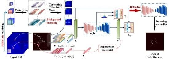
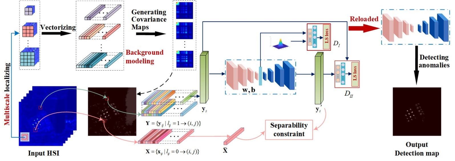
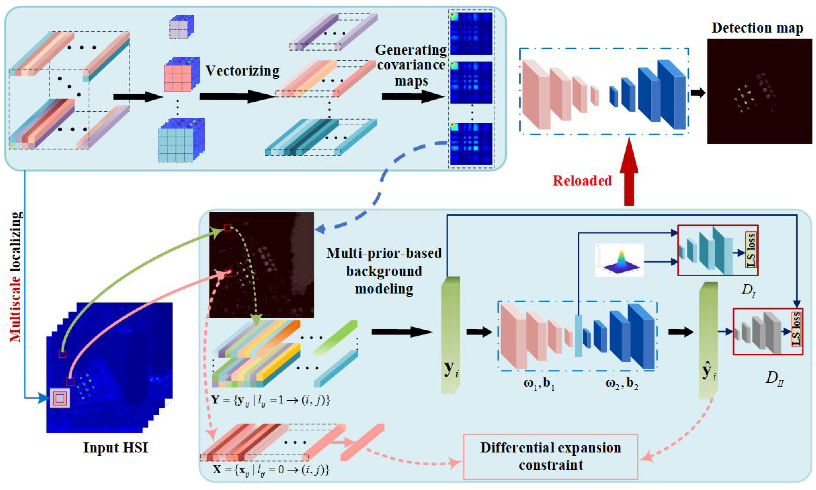
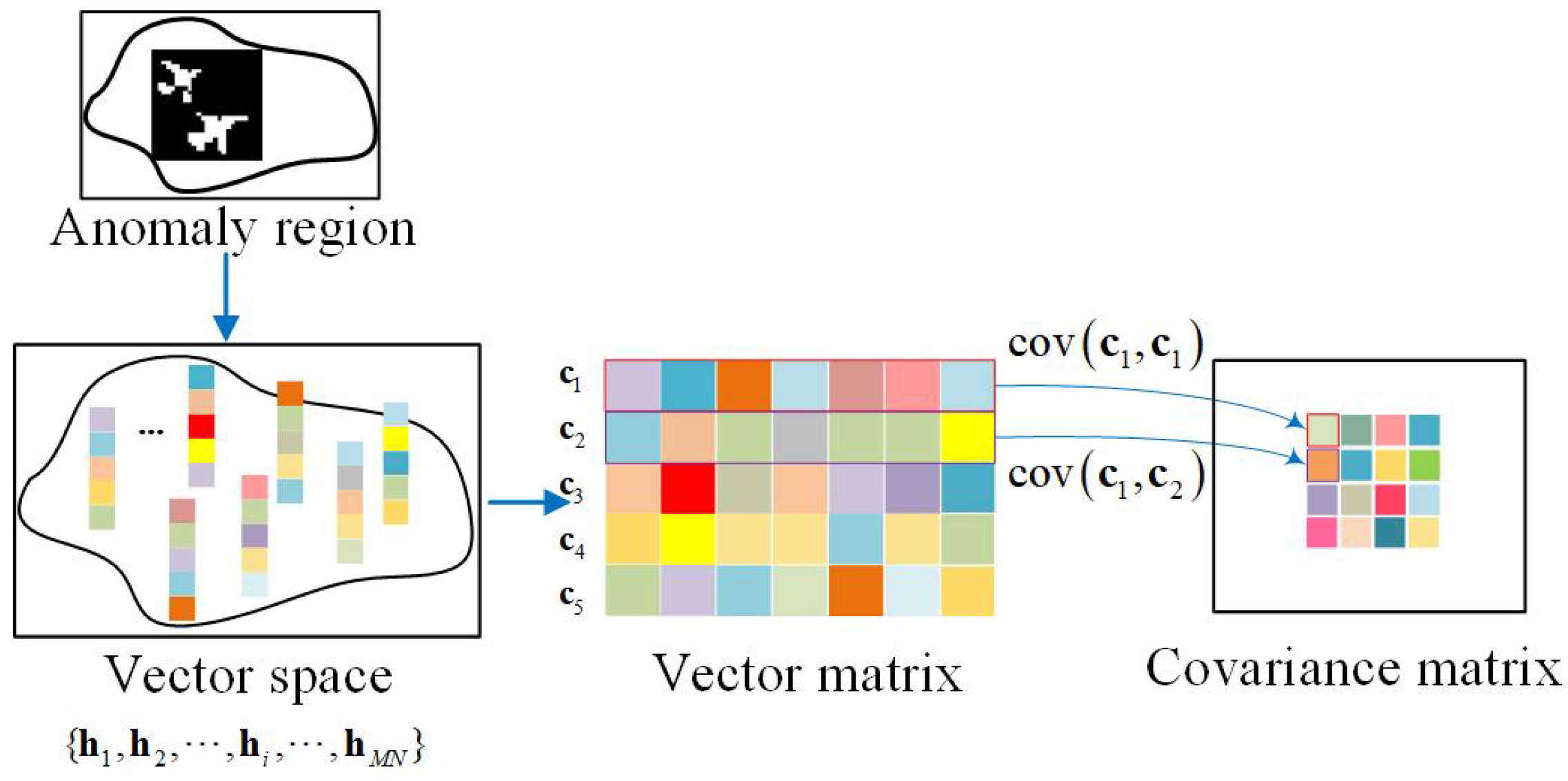
  • To change the preconceptions of anomaly detection with insufficient samples, we propose a multi-prior strategy to reliably and adaptively generate prior dictionaries. Specifically, we calculate a series of multi-scale covariance matrices rather than traditional one-order statistics, taking advantage of second-order statistics to naturally model the distribution with integrated spectral and spatial information.
  • The twin least-square loss in both the feature and image domains and differential expansion loss are jointly introduced into the architecture to fit the characteristics of high-dimensional and complex HSI data, which can overcome the gradient vanishing and training stability problem.
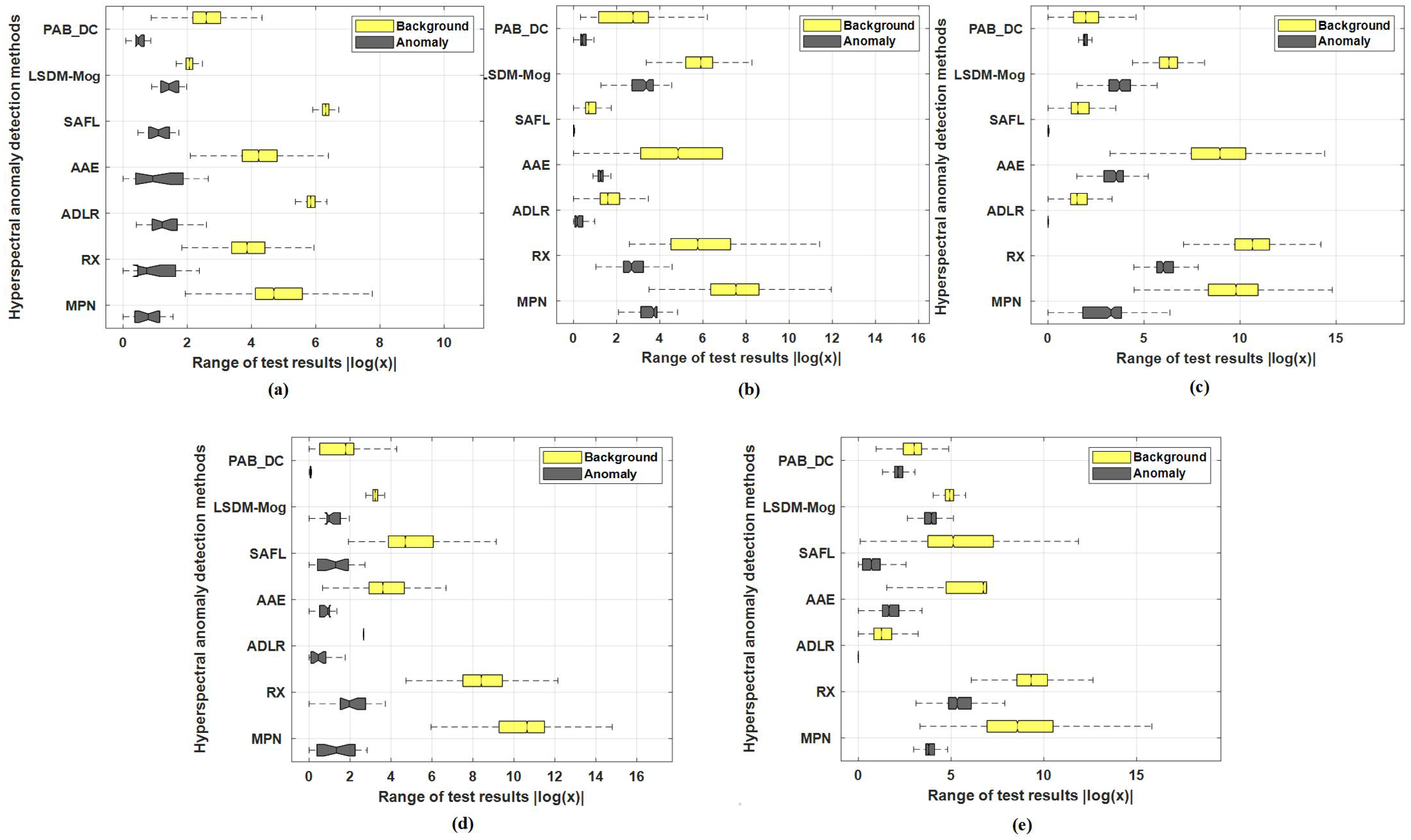
  • To lease the generation ability of the model and reduce the false-alarm rate by an order of magnitude, we design a weakly supervised training pattern to enlarge the distribution diversity between background regions and anomalies, aiming to distinguish between background and anomalies in reconstruction. Experimental results illustrate that the AUC score of P f , τ in MPN is one order of magnitude lower than other compared methods.
We divide the remainder of this paper into four sections. The hyperspectral anomaly detection and generative adversarial networks are reviewed in Section 2. The MPN methodology is concretely described in Section 3. In Section 4, we represent experiments and discuss the results. In Section 5, we draw our conclusions.

2. Related Work

2.1. Hyperspectral Anomaly Detection

Recently, plenty of anomaly-detection methods have been developed. The statistics-based methods and sparsity-based methods are two representative categories [31,32]. There are mainly two categories for traditional hyperspectral anomaly detection approaches, the first of which comprises RX-based algorithms [33]. The RX detector is based on the assumption that each spectral channel obeys Gaussian distribution. The non-RX-based methods include collaborative representations, sparse representations, and low-rank representations. The ADLR method obtains abundance vectors by spectral decomposition. It constructs a dictionary based on the mean value clustering of abundance vectors [34]. The low-rank and sparse constraints are imposed in the PAB_DC model in consideration of the homogeneity of background and the sparsity of anomalies to construct the background and potential anomaly dictionaries [35]. The emerging typical algorithm for background removal is AED, which removes the background by attribute filtering and difference operation [36]. Additionally, unlike single distribution modeling in traditional LSDM, the LSDM–MoG method combines the mixed-noise models and low-rank background to characterize complex distributions more accurately [37].

2.2. Generative Adversarial Networks (GANs)

By improvement of generation quality and training stability, generative adversarial networks (GANs) perform advanced image generation ability [38,39,40,41]. The capability of high-quality image generation accounts for the application of GANs to many image processing tasks [42,43]. For hyperspectral anomaly detection, existing works based on deep learning focus mainly on feature extraction or dimension reduction. With small input samples, limited by difficulties in annotation and collection of label training, supervised or semi-supervised methods aim to make a tradeoff between sample numbers and detection performance. However, they still require hard-to-attain pure background training samples for representation. Unsupervised learning has become a new trend, but detection accuracy is unsatisfactory with insufficient prior knowledge. Moreover, complex characteristics of HSIs in real scenarios are not yet fully considered or plugged into the network. In contrast, the proposed MPN aims to address these issues while maintaining a good performance.

3. Proposed Method

In this work, we elaborate on MPN for hyperspectral anomaly detection. The whole process is shown in Figure 1. We denote the HSI as H R h × w × d . The number of the spectral bands is denoted by d. The spatial size of the data is described by h and w. For convenience, as the input of the network, the 3D cube H is converted into a 2D matrix H = h i i = 1 n R d × n . Each column of H is a spectral pixel vector in the HSI. n = h × w is the number of the pixels. The HSI data matrix can be decomposed into two parts—background and anomaly—which are denoted as Y = y 1 , y 2 , , y n B , X = x 1 , x 2 , , x n A , respectively, where n A + n B = n . y i represents the ith vector in Y , i = 1 , 2 , , n A . x i represents the ith vector in X , i = 1 , 2 , , n B . Furthermore, the reconstructed background spectral is denoted as Y ^ = σ W W T Y + B , where σ · represents the activation function. Y ^ is the output of the network, and W is the weight of the encoder. B is the bias of the whole network. The pixel can be represented by the combination of other surrounding background pixels since there is a correlation between background pixels. The linear decomposition model of HSI is formulated as
H = B 0 W + A 0 + N ,
where B 0 W is the background component; B 0 = b 1 , b 2 , , b n B are the background dictionaries; W = w 1 , w 2 , , w n are the corresponding representation coefficients; and A 0 = a 1 , a 2 , , a n a is anomaly component. For simplicity, we consider N as zero.
Different from the previous single-distribution-based anomaly-detection method RX, we calculate the covariance between the two vectors by estimating the probabilities of the testing pixel belong to the anomaly class by calculating the Mahalanobis distance with neighboring pixels. Inspired by the distance-based method and the multi-scale approach [44,45], we consider that, through background dictionaries modeling, the constructed covariance maps can reuse the MCMs and represent the spatial and spectral information of HSI as the prior for GAN training. Thus, the decomposition can be regarded as a nonlinear problem, which has the following expression:
H = f M C M B , A
where f M C M · represents the learning process of MCM algorithm. A and B denote the background and anomaly dictionaries, respectively.

3.1. Network Architecture

Instead of single-scale Gaussian distribution with a generative adversarial network method, we present a deep network, i.e., MPN, to directly model the complex HSI and its dictionary, which characterizes the essential attribute of HSI implicitly. In this way, both the multi-prior dictionary scheme and the jointly separable loss can contribute to detecting the anomalies from the complex HSI data in a weakly supervised pattern. Thus, according to the defined dictionaries, the anomaly-detection task can be formulated as
L Y , X = L T L S Y + L a u Y , Y ^ + L e n Y ^ , X = L L S 1 Z + L L S 2 Y , Y ^ + Y Y ^ α Y ^ X ,
s . t . Z = E n c Y ; arg ( G ) Y ^ = D e c Z ; arg ( D ) α N 0 , I ,
where Y ^ is decoder output, and Z is the latent feature as encoder output. The twin least-square loss L T L S added for the two discriminators are denoted by L L S 1 and L L S 2 , respectively, which make up the whole least-square-based loss L T L S . L a u represents the spectral reconstruction loss, which is aimed at mapping the input to the output space. L e n denotes the separability loss between background and anomaly dictionary which aims to enlarge the difference, respectively. Y Y ^ denotes the reconstruction error of basic generative adversarial network. E n c and D e c represent the encoder and decoder, respectively.

3.2. Multi-Prior for Background Construction

We generate pseudo priors for GAN training through multi-scale covariance map construction. This strategy was inspired by the estimation of the Mahalanobis distance between the test pixels and the constructed pixels on one scale. Thus, we can obtain sufficient prior information and take advantage of both the spatial and spectral information of HSI. The progress of multi-prior construction strategy is shown in Figure 2.

3.2.1. Multi-Scale Localizing

For each central pixel, we try to realize multi-scale localizing first based on the Euclidean distance with a classical classifier, i.e., K nearest neighbors (KNN), to obtain the local pixel cubes at different scales. Then, we generate a series of gradually increasing cubes of different scales. For each of the cubes, we transfer it to a vector. After that, the covariance matrix is calculated between the vectors. Furthermore, we take into account the situation of M scales T k , k = 1 , , M . Thus, the extraction of M covariance maps are attained to represent the center pixel x k , denoted by C k , respectively. Additionally, for the central pixel h i , taking the scale R × R as an example, the covariance map of h i on the fixed one scale is extracted as
C k = 1 R 2 1 i = 1 R 2 h i μ h i μ T R L × L ,
where μ represents the mean of input HSI vectors h i | i = 1 , 2 , , R . Furthermore, h i | i = 2 , , R 2 represents the corresponding adjacent pixels in a window of R × R pixels. In addition, we extend to M scales of R k , i.e., k = 1 , , M . We denote the covariance maps of other scales as C k , k = 1 , , M , which make up the covariance pool to construct the background.

3.2.2. Generating Covariance Maps

Aiming at the original pixel, we construct a series of increasingly larger cubes in consideration of the increasing window size of the spatial neighborhood around each one. Furthermore, for each of these cubes, after vectorizing, we calculate the CM of the two vectors to represent the information contained in the central pixel and enhanced by considering gradually expanding neighborhoods. Such CMs obtained from increasingly larger spatial proportions are denoted by MCM, which can be used to train the detector more effectively.

3.3. Two-Branch Cascaded Architecture with Least-Square Losses

Though GAN performs well in anomaly-detection tasks according to the literature [45], the real objective of GAN is supposed to capture more separable latent features between background and anomalies instead of minimizing the pixel-wise reconstruction error. Additionally, conventional GAN style architectures obtain blurry reconstructions because of multiple modes in the actual normal distribution falsifying reconstruction errors. Moreover, the unstable training process and limitation of the capacity of GAN-style architecture remain to be improved.
Therefore, we propose a twin least-square GAN under the semi-supervised pattern with background vectors reconstructed to address the above issues. Compared with conventional GANs, an auxiliary discriminator, anomaly rejection loss, and least-square losses are adopted to the framework. The anomaly rejection loss aims to gather the latent background dictionaries and make them more concentrated. Thus, the differentiation between the background and anomalies can be enlarged. Additionally, the auxiliary image discriminator plays a role in achieving a better balance in the training process.

3.3.1. Stability Branch

When the generator is updated, the non-saturation loss and min–max loss will hardly lead to gradients to false samples since the fake samples still differ from the real data [40]. To solve the problem, we consider the least-squares loss to penalize the samples which are far from the decision boundary, even if they are on the right side. We introduce least-squares loss to move false vectors to the decision boundary. The least-square loss added network can reconstruct vectors that are similar to the real data. Furthermore, the vanishing gradient is alleviated while the GANs learning is more stable. Thus, we introduce least-square losses to the architecture and define them in both the two discriminators with enhanced background anomaly discrimination from the input space to the reconstructed one. Consequently, the background spectral vectors are adequately and stably estimated with better performance. The objective function of the least-squares-loss-based network can be expressed as follows.
min G V L S ( G ) = 1 2 E x p d a t a ( x ) [ ( D ( x ) n ) 2 ] + 1 2 E z p z ( z ) [ ( D ( G ( z ) ) m ) 2 ]
min D V L S ( D ) = 1 2 E x p d a t a ( x ) [ ( D ( x ) l ) 2 ] + 1 2 E z p z ( z ) [ ( D ( G ( z ) ) l ) 2 ]
where m and n are the labels for fake and real data, respectively. Furthermore, l denotes the value that G wants D to believe for fake data. As shown in Figure 1, the MPN architecture contains one generator and two discriminators. The generator network includes the encoder E n and decoder D e . Firstly, the mapping relationship between input background dictionaries and the network output can be regarded as the mapping function. The training objective of L Y , D R , D F , G is to capture the distribution of background dictionaries in both the reconstructed and deep-spectrum vector space. Motivated by this, L Y , D R , D F , G intends to produce a minimum anomaly score for background, but a higher score for the anomaly. To achieve this goal, in addition to the basic reconstruction loss in the equation, we also add spatial adversarial loss, potential spatial adversarial loss, and anomaly rejection loss, which all contribute to the whole learning objective.
Considering the discriminator as a classifier, the sigmoid cross-entropy loss function is adopted in regular basic GANs. When updating the generator, the loss function will cause vanishing gradients because the samples on the correct side of the decision boundary are still far from the real data. To remedy this problem, we introduce the least-square loss function into the architecture. As shown in Figure 1, the MPN network consists of two discriminators and a generator. The twin least-square loss can be expressed as
L L S 1 = 1 2 E y p d a t a ( y ) [ ( D F ( y ) 1 ) 2 ] + 1 2 E z p z ( z ) [ ( D F ( G ( z ) ) + 1 ) 2 ] ,
L L S 2 = 1 2 E y p d a t a ( y ) [ ( D R ( y ) 1 ) 2 ] + 1 2 E y ^ p y ^ ( y ^ ) [ ( D R ( G ( y ^ ) ) + 1 ) 2 ] ,
From the binary classification point of view, we introduce the twin least-square loss to move false samples to the decision boundary of being anomaly or background. Thus, we perform adversarial training on the two least-square-loss imposed discriminators D R and D F against the generator. Consequently, the problem of gradient vanishing can be overcome and the consistency with the distribution of the reconstructed y ^ and the input data y can be ensured.

3.3.2. Separability Branch

As mentioned earlier, we impose the spectral reconstruction loss using mean squared error (MSE) so that the deviation between the reconstructed and the input can be optimized:
L a u Y , Y ^ = Y Y ^ = Y σ W W T Y + B ,
To ensure that the learning samples come entirely from the background, we introduce the following distance function based on L a u . The second item of this is expected to be as large as possible:
L a n Y , Y ^ = L a u Y , Y ^ + L e n Y ^ , X = Y Y ^ α Y ^ X = Y σ W W T Y + B α σ W W T Y + B X ,
Let x i and y i represent the ith component in X and Y , respectively. x ¯ denotes the mean of all the x i in X . When the distance between the reconstructed spectrum vector y ^ i and the average spectrum vector x ¯ are small, y i is suspected to be an anomaly vector. Then, the suppression coefficient α of the function aims to reduce it rapidly for adjustment. When the distance between x ¯ and y i is large, from a statistical point of view, y i is the background dictionary to be estimated. Then, the value of the suppression coefficient α is approximately 1.

3.4. Solving the Cascaded Model

The twin least-square loss, spectral reconstruction loss, and differential expansion loss are jointly learned with the weighting coefficient of 1 by carrying out alternative updates of each component as follows. Subsequently, we obtain the detection maps by Gaussian-statistics-based discrimination.
  • Minimize L L S 1 by updating parameters of D F .
  • Minimize L L S 2 by updating parameters of D R .
  • Minimize L a n by updating parameters of E n and the decoder D e .
where the first discriminator D F with the least-square loss aims to reduce gradient vanishing in the latent space. The second D R with the least-square loss tries to reconstruct images to approximate the input in the reconstructed image space. The model is trained using the Adam optimization algorithm by carrying out alternative updates of each component. Then we re-adopted the multi-prior algorithm on reconstruction results as follows.
J = y ^ i μ T C y ^ i μ .
where μ denotes the mean vector and C represents the multi-prior of the reconstructed H ^ , respectively.

4. Experimental Results and Discussion

We design and execute experiments to verify the effectiveness of the proposed model. We qualitatively and quantitatively compared and analyzed the detection results of the MPN method with six state-of-the-art algorithms.

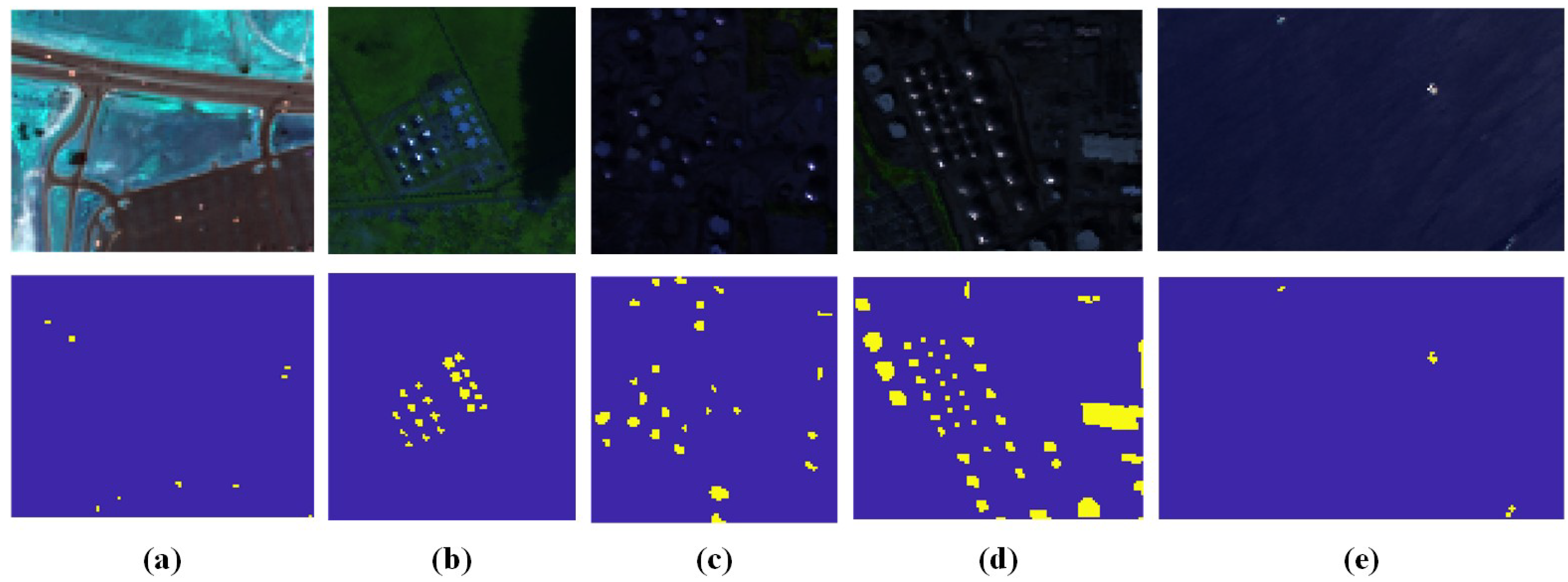
4.1. Datasets Description

The tested HSIs captured at different scenes are described for performance evaluation of the MPN and compared methods. The pseudo-color images and ground truth of the datasets are shown in Figure 3. There are part of the datasets provided online to access (http://xudongkang.weebly.com/data-sets.html (accessed on 6 May 2022)).

4.1.1. HYDICE

Captured by the hyperspectral digital image acquisition experiment (HYDICE) airborne sensors above the city, the first dataset describes urban scenes in the United States. There are 162 spectral channels in the original image with a wavelength from 400 to 2500 nanometers (nm). From the entire original image, a sub-image with a space size of 80 × 100 is cropped. In the spectral band, 162 bands are reserved. The total number of anomalous pixels is 19. The anomaly pixels represent cars and roofs.

4.1.2. Airport–Beach–Urban (ABU) Database

The airplane, city, and most beach scenes of the second dataset are recorded by the airborne visible/infrared imaging spectrometer (AVIRIS) sensors. One of the datasets in the beach scene is captured by the Reflective Optics System Imaging Spectrometer (ROSIS-03) sensor. The AVIRIS instrument contains 224 different detectors, each with a spectral bandwidth of approximately 10 nm, allowing it to cover the entire range between 380 and 2500 nm (http://aviris.jpl.nasa.gov/ (accessed on 6 May 2022)). The sample image with a size of 100 × 100 is manually extracted from the large image. The datasets are available online and can be downloaded from the AVIRIS website.

4.1.3. Grand Island

The Grand Island dataset was also acquired by the AVIRIS sensor. It was captured at the location of GrandIsland on the Gulf Coast. In spatial domain, it contains 300 × 480 pixels. While in spectral domain, it contains 224 spectral channels with a wavelength range of 366–2496 nm.

4.1.4. EI Segundo

The EI Segundo dataset was captured by AVIRIS sensors. The structure of the refinery is regarded as an anomaly to be detected. It has 250 × 300 pixels in the spatial domain. In the spectral domain, the band number is 224, ranging from 370 to 250 nm.

4.2. Evaluation Metrics

Let P d , P f , and τ represent the true positive rate, false positive rate, and threshold, respectively. We introduce the receiver operating characteristic curve (ROC) together with the area under it to quantitative evaluation. The area under the ROC curve of P d , P f demonstrates the detection accuracy. The closer this value is to 1, the better the detection capability. In contrast, the closer the area value under the P f , τ is to 0, the better the false alarm rate.

4.3. Experiment Setup

Our model is built on the basic GAN model, which is composed of encoder, decoder, and discriminators. We set the training iteration to 5000. The learning rate is chosen to be 0.0001 to balance the performance and iteration speed. There are three layers for each part. We set the number of the extracted feature to 20 after ranging the value from 10 to 100 for all the datasets. With a proper number of 20, the proposed model can represent an extracted feature well for the input spectral and promote the detection performance. We optimize all parameters by the Adam optimization algorithm with backpropagation. Varying from 30 to 50, the size of windows make the detection results differ from each other. It achieves the optimal accuracy when the size is set to between 15 and 25. Similarly, we set the value of the scales of multi-scale covariance maps as 5 to make a balance between the performance and the computation costs for the tested datasets. For the parameter settings of compared methods, the RX method is parameter-free by design. Other algorithms require parameters tuning to achieve upper bounds on the performance. For the Grand Island and Segundo datasets, the main parameters s is set to 10, and r is set to 0.6. There are two main parameters in the ADLR method. We set the c between 20 and 30. The b w varies from 0.2 to 0.55. Furthermore, l a m b d a is set between 0.01 and 0.1. In the PAB_DC method, we select the parameters according to [35]. The LSDM–MoG algorithm uses a combination of mixed-noise models and low-rank backgrounds to more accurately characterize complex distributions. The parameter setting is consistent with [37]. In AAE, the three layers of each sub-network obtain 500, 500, and 20 units, respectively, [38]. In SAFL, the batch size is set as the number of spatial pixels of HSI. The training epoch is set to 10,000. The learning rates are set to 0.001 and 0.0001, respectively, for the encoder, decoder, and discriminator [39].

4.4. Ablation Study

To better understand the effect of each component on output detection result in MPN, we analyzed the performances under the following four scenes of training models: (1) MPN without multi-prior module; (2) MPN without twin least-square loss module; (3) MPN without differential expansion loss; (4) MPN.
From Table 1 and Table 2, it can be concluded that the MPN achieves a higher AUC score of P d , P f and a lower AUC score of P f , τ than other models. The AUC score of P d , P f on average compared with other configurations are improved by about 0.276%, 0.266%, and 0.156%, respectively. Furthermore, the AUC score of P f , τ on average are optimized by about 10.425%, 6.950%, and 1.351%, respectively. The results indicate the effectiveness and necessity of multi-prior, twin least-square loss, and differential expansion loss, which contribute effectively to improve the detection performance.

4.5. Discussion

4.5.1. Baseline Methods

We compare the performance with five commonly used methods according to their open-source codes and literature, including RX, PAB_DC, AAE, ADLR, SAFL, and LSDM–MoG. To further validate the effectiveness of the multi-scale covariance maps (MCMs) and least-square loss, the experiments were conducted on several public and widely used real-world HSI datasets, i.e., HYDICE, ABU datasets, Grand Island, EI Segundo datasets.

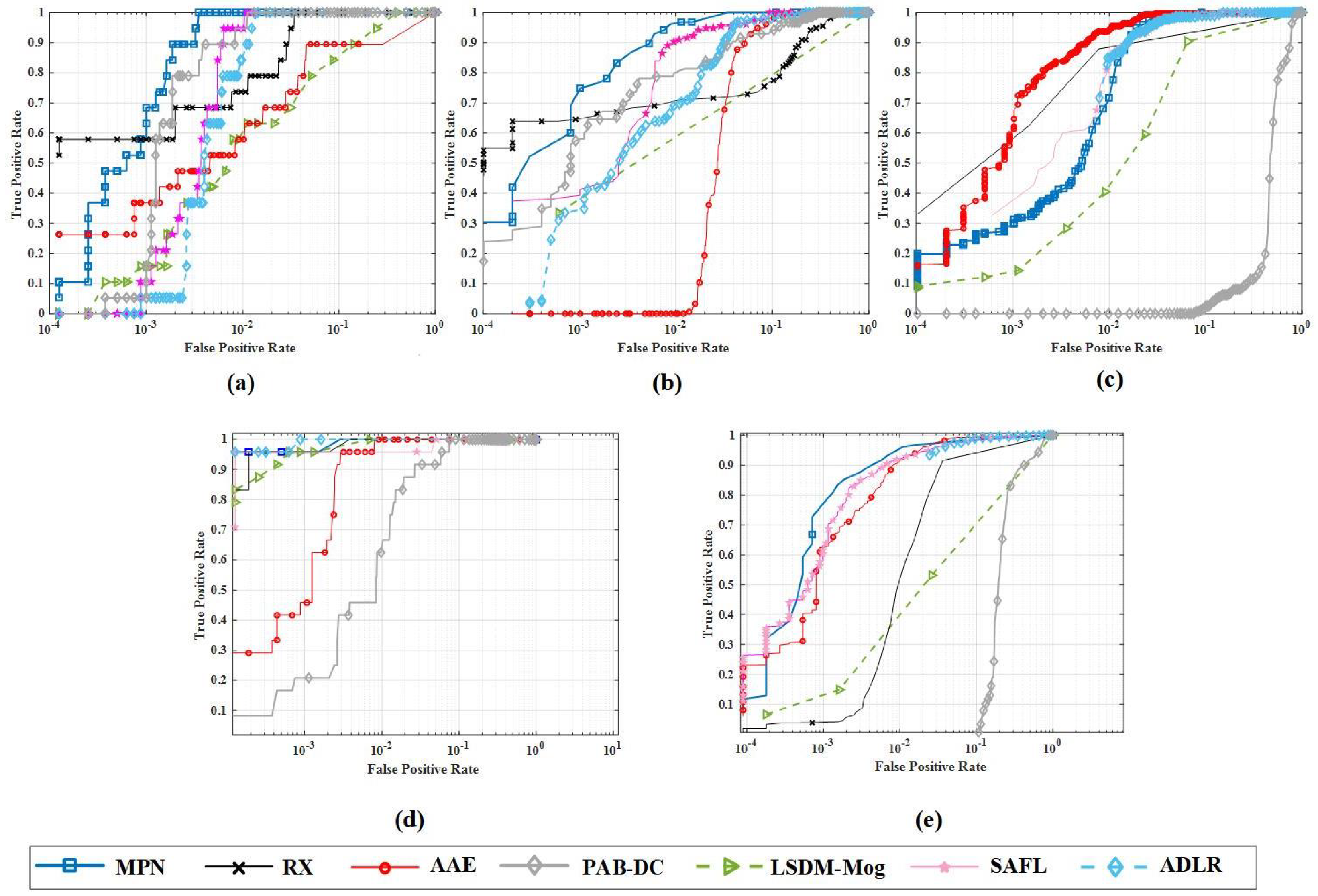
4.5.2. Quantitative Comparison

The quantified AUC scores of P d , P f , and P f , τ are listed in Table 3 and Table 4, respectively. Relative to the AUC score of P d , P f , MPN exceeds the well-performed methods ADLR and RX for about 0.493% and 1.063% on average, respectively. More notably, its AUC score of P f , τ is mostly an order of magnitude less than that of others. Specifically, the average AUC score of P d , P f of the proposed method is 0.99809. In comparison, the result of the second best method ADLR of 0.99321, with lower AUC scores of P f , τ of 0.00518 compared with 0.05096. It can be concluded that the MPN method shows promising background suppression ability for most of the scene and better detection accuracy for small and embedded anomalies. Generally speaking, the comparison methods may achieve good results for some specific datasets, while MPN can achieve promising detection results in both indexes for all the datasets, which can also be reflected on the ROC curves of P d , P f in Figure 4, respectively. To further verify the background suppression and target detection ability, we also perform the separation analysis through a boxplot. The detection results of all the detectors on different datasets are shown in Figure 5. The distance between the upper boundary of the yellow box and the lower boundary of the gray box indicates the separability of the background anomaly, in which the MPN obtains better discrimination results on most datasets among the compared methods.

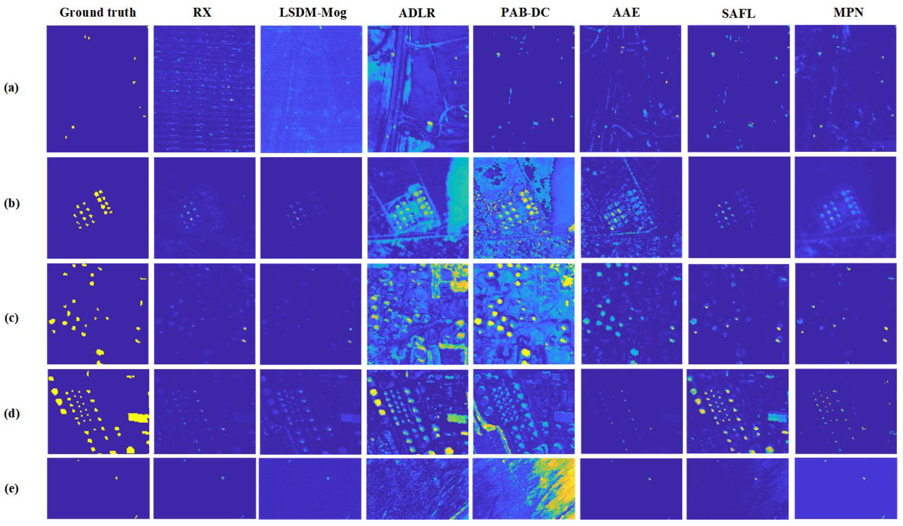
4.5.3. Qualitative Comparison

For the ABU-urban1 dataset, the MPN performs well in detection, especially in some small-sized anomalies with higher intensity. Meanwhile, the false-alarm rate is restricted to a lower level in urban scenes. The RX, AAE, and ADLR methods can exactly locate the anomalies. However, the spatial shape preservation is not good enough. As for LSDM–MoG and PAB_DC methods, the anomalies are detected although the edges information around anomalies is not well obtained. For the ABU-urban2 dataset, the ADLR and the MPN can detect anomalies well and lower false-alarm rate. The AAE method presents a good ability in detecting all anomalies, but the intensity is relatively high. In RX and ADLR methods, the background suppression ability performs well but some pixel-level anomalies are relatively blurred. For the LSDM–MoG method, some of the anomalies are lost and cannot be figured out visually. The RX, LSDM–MoG, and PAB_DC methods perform well on the Grand Island dataset in detection accuracy, but they suffer from the interference of the complex background. The ADLR method can avoid false alarms, but some edge details are not obtained. Both AAE and the MPN method can protect anomalies with high detection accuracy and low false-alarm rates. In Figure 6, it can be observed that the PAB_DC method for HYDICE dataset keeps targets relatively clearly although some part of anomalies is missed. In ADLR and LSDM–MoG methods, most anomalies are visually mixed with the background. RX can detect almost all anomalies with high intensity. However, the suppression ability of background interference is not effective. Both PAB_DC and the MPN method can suppress the background well and obtain high detection accuracy. For the Segundo dataset, MPN can well detect the anomalies in the scene among the compared methods with the best results. The RX, AAE, and ADLR methods have favorable identification of the location of the anomalies but lost some of the shape information. In conclusion, the MPN represents promising performance with the detection maps closest to the ground truths.

5. Conclusions

In this work, a novel multi-prior strategy and joint separable loss scheme embedded network is proposed for anomaly detection of HSI. Some points of our work deserve consideration. For the first time, we propose the multi-prior strategy to construct multi-scale prior information and reuse the covariance map at multiple scales to adaptively create reliable and stable priors. Therefore, we can solve the lack of priors with pseudo-labeling and fully take advantage of spectral and spatial information. To overcome the problem of gradient vanishing and improve the generative ability during training, we introduce twin least-square loss to the network in both feature and image domains. Finally, the differential expansion loss added MPN establishes a pure and discriminative background estimation, separating the background and the anomalous spectral vectors to a greater extent. Through experiments, we have proved that the MPN exhibits superior performance in background reconstruction and outperforms the state-of-the-art methods.

Author Contributions

J.Z., Y.L. and W.X. provided the conceptualization of the work, designed the methodology, and conducted the experiments; Y.L., W.X., J.L. and X.J. gave advice on optimization and reviewed the manuscript; writing, J.Z. All authors have read and agreed to the published version of the manuscript.

Funding

This work was supported in part by the National Natural Science Foundation of China under Grant 62121001, Grant 62071360, and Grant 61801359.

Data Availability Statement

Publicly available datasets were analyzed in this study. The ABU dataset can be found here: [http://xudongkang.weebly.com/data-sets.html accessed on 6 May 2022]. The Grand Island and EI Segundo datasets are obtained from Xudong Kang. We would like to express our appreciation to Xudong Kang for providing these datasets.

Conflicts of Interest

The authors declare no conflict of interest.

Abbreviations

The following abbreviations are used in this manuscript:
GANsgenerative adversarial networks
HSIhyperspectral imagery
MCMsmulti-scale covariance maps
KNNK nearest neighbors
MSEmean squared error
ROCthe receiver operating characteristic curve

References

  1. Camps-Valls, G.; Tuia, D.; Bruzzone, L.; Benediktsson, J. Advances in hyperspectral image classifification: Earth monitoring with statistical learning methods. IEEE Signal Process. Mag. 2013, 31, 45–54. [Google Scholar] [CrossRef] [Green Version]
  2. Okwuashi, O.; Christopher, E. Deep support vector machine for hyperspectral image classification. Pattern Recognit. 2020, 103, 107298. [Google Scholar] [CrossRef]
  3. Yan, X.; Zhang, H.; Xu, X.; Hu, X.; Heng, P. Learning semantic context from normal samples for unsupervised anomaly detection. In Proceedings of the AAAI Conference on Artificial Intelligence (AAAI), Virtual, 8 February 2021; p. 425. [Google Scholar]
  4. Abati, D.; Porrello, A.; Calderara, S.; Rita, C. Latent space autoregression for novelty detection. In Proceedings of the IEEE Conference on Computer Vision and Pattern Recognition (CVPR), Long Beach, CA, USA, 15–20 June 2019; pp. 481–490. [Google Scholar]
  5. Ma, M.; Mei, S.; Wan, S.; Hou, J.; Wang, Z.; Feng, D. Video summarization via block sparse dictionary selection. Neorocomputing 2020, 378, 197–209. [Google Scholar] [CrossRef]
  6. Luo, W.; Liu, W.; Lian, D.; Tang, J.; Gao, S. Video anomaly detection with sparse coding inspired deep neural networks. IEEE Trans. Pattern Anal. Mach. Intell. 2019, 43, 1070–1084. [Google Scholar] [CrossRef]
  7. Stanislaw, J.; Maciej, S.; Stanislav, F.; Devansh, A.; Jacek, T.; Kyunghyun, C.; Krzysztof, G. The break-even point on optimization trajectories of deep neural networks. In Proceedings of the International Conference on Learning Representations (ICLR), Addis Ababa, Ethiopia, 26–30 April 2020. [Google Scholar]
  8. Chalapathy, R.; Chawla, S. Deep learning for anomaly detection: A survey. arXiv 2019, arXiv:1901.03407. [Google Scholar]
  9. Eyal, G.; Aryeh, K.; Sivan, S.; Ofer, B.; Oded, S. Temporal anomaly detection: Calibrating the surprise. In Proceedings of the AAAI Conference on Artificial Intelligence (AAAI), Honolulu, HI, USA, 27 January–1 February 2019; pp. 689–692. [Google Scholar]
  10. Wen, T.; Keyes, R. Time series anomaly detection using convolutional neural networks and transfer learning. In Proceedings of the International Joint Conference on Artifificial Intelligence (IJCAI), Macao, China, 10–16 August 2019. [Google Scholar]
  11. Ansari, A.; Scarlett, J.; Soh, H. A characteristic function approach to deep implicit generative modeling. In Proceedings of the IEEE Conference on Computer Vision and Pattern Recognition (CVPR), Seattle, WA, USA, 13–19 June 2020; pp. 7478–7487. [Google Scholar]
  12. Villa, A.; Chanussot, J.; Benediktsson, J.; Jutten, C.; Dambreville, R. Unsupervised methods for the classifification of hyperspectral images with low spatial resolution. Pattern Recognit. 2013, 46, 1556–1568. [Google Scholar] [CrossRef]
  13. Fowler, J.; Du, Q. Anomaly detection and reconstruction from random projections. IEEE Trans. Image Process. 2011, 21, 184–195. [Google Scholar] [CrossRef] [Green Version]
  14. Gong, Z.; Zhong, P.; Hu, W. Statistical loss and analysis for deep learning in hyperspectral image classifification. IEEE Trans. Neural Netw. Learn. Syst. 2020, 32, 322–333. [Google Scholar] [CrossRef] [Green Version]
  15. Zhang, L.; Cheng, B. A stacked autoencoders-based adaptive subspace model for hyperspectral anomaly detection. Infrared Phys. Technol. 2019, 96, 52–60. [Google Scholar] [CrossRef]
  16. Erfani, S.; Rajasegarar, S.; Karunasekera, S.; Leckie, S.; Leckie, C. High dimensional and large-scale anomaly detection using a linear one-class SVM with deep learning. Pattern Recognit. 2016, 58, 121–134. [Google Scholar] [CrossRef]
  17. Wang, L.; Xiong, Z.; Shi, G.; Wu, F.; Zeng, W. Adaptive nonlocal sparse representation for dual-camera compressive hyperspectral imaging. IEEE Trans. Pattern Anal. Mach. Intell. 2016, 39, 2104–2111. [Google Scholar] [CrossRef] [PubMed]
  18. Velasco-Forero, S.; Angulo, J. Classification of hyperspectral images by tensor modeling and additive morphological decomposition. Pattern Recognit. 2013, 46, 566–577. [Google Scholar] [CrossRef] [Green Version]
  19. Malpica, J.; Rejas, J.; Alonsoa, M. A projection pursuit algorithm for anomaly detection in hyperspectral imagery. Pattern Recognit. 2008, 41, 3313–3327. [Google Scholar] [CrossRef]
  20. Wang, Z.; Li, Y.; Guo, Y.; Fang, L.; Wang, S. Data-uncertainty guided multiphase learning for semi-supervised object detection. In Proceedings of the IEEE Conference on Computer Vision and Pattern Recognition (CVPR), Nashville, TN, USA, 20–25 June 2021. [Google Scholar]
  21. Taghipour, A.; Ghassemian, H. Unsupervised hyperspectral target detection using spectral residual of deep autoencoder networks. In Proceedings of the International Conference on Pattern Recognition and Image Analysis (IPAS), Tehran, Iran, 6–7 March 2019; pp. 52–57. [Google Scholar]
  22. Liu, Y.; Li, Z.; Zhou, C.; Jiang, Y.; Sun, J.; Wang, M.; He, X. Generative adversarial active learning for unsupervised outlier detection. IEEE Trans. Knowl. Data Eng. 2019, 32, 1517–1528. [Google Scholar] [CrossRef] [Green Version]
  23. Yang, X.; Dong, M.; Wang, Z.; Gao, L.; Zhang, L.; Xue, J. Data-augmented matched subspace detector for hyperspectral subpixel target detection. Pattern Recognit. 2020, 106, 107464. [Google Scholar] [CrossRef]
  24. Ergen, T.; Kozat, S. Unsupervised anomaly detection with LSTM neural networks. IEEE Trans. Neural Netw. Learn. Syst. 2020, 31, 3127–3141. [Google Scholar] [CrossRef] [Green Version]
  25. Wu, H.; Prasad, S. Semi-supervised deep learning using pseudo labels for hyperspectral image classifification. IEEE Trans. Image Process. 2018, 27, 1259–1270. [Google Scholar] [CrossRef]
  26. Antonio, P.; Atli, B.; Jason, B.; Lorenzo, B.; Gustavo, C.; Jocelyn, C.; Mathieu, F.; Paolo, G.; Anthony, G. Recent advances in techniques for hyperspectral image processing. Remote Sens. Environ. 2009, 113, S110–S122. [Google Scholar]
  27. Yang, X.; Deng, C.; Zheng, F.; Yan, J.; Liu, W. Deep spectral clustering using dual autoencoder network. In Proceedings of the IEEE Conference on Computer Vision and Pattern Recognition (CVPR), Long Beach, CA, USA, 15–20 June 2019; pp. 4066–4075. [Google Scholar]
  28. Dincalp, U.; G zel, M.; Sevine, O.; Bostanci, E.; Askerzade, I. Anomaly based distributed denial of service attack detection and prevention with machine learning. In Proceedings of the 2018 2nd International Symposium on Multidisciplinary Studies and Innovative Technologies (ISMSIT), Ankara, Turkey, 19–21 October 2018; pp. 1–4. [Google Scholar]
  29. Wang, R.; Guo, H.; Davis, L.; Dai, Q. Covariance discriminative learning: A natural and efficient approach to image set classification. In Proceedings of the IEEE Conference on Computer Vision and Pattern Recognition (CVPR), Providence, RI, USA, 16–21 June 2012; pp. 2496–2503. [Google Scholar]
  30. He, N.; Paoletti, M.; Haut, J.; Fang, L.; Li, S.; Plaza, A.; Plaza, J. Feature extraction with multiscale covariance maps for hyperspectral image Classification. IEEE Trans. Geosci. Remote Sens. 2019, 57, 755–769. [Google Scholar] [CrossRef]
  31. Li, A.; Miao, Z.; Cen, Y.; Zhang, X.-P.; Zhang, L.; Chen, S. Abnormal event detection in surveillance videos based on low-rank and compact coefficient dictionary learning. Pattern Recognit. 2020, 108, 107355. [Google Scholar] [CrossRef]
  32. Fang, L.; He, N.; Li, S.; Plaza, A.; Plaza, J. A new spatial-spectral feature extraction method for hyperspectral images using local covariance matrix representation. IEEE Trans. Geosci. Remote Sens. 2018, 56, 3534–3546. [Google Scholar] [CrossRef]
  33. Reed, I.; Yu, X. Adaptive multiple band CFAR detection of an optical pattern with unknown spectral distribution. IEEE Trans. Acoust. Speech Signal Process. 1990, 38, 1760–1770. [Google Scholar] [CrossRef]
  34. Qu, Y.; Wang, W.; Guo, R.; Ayhan, B.; Kwan, C.; Vance, S.; Qi, H. Hyperspectral anomaly detection through spectral unmixing and dictionary-based low-rank decomposition. IEEE Trans. Geosci. Remote Sens. 2018, 56, 4391–4405. [Google Scholar] [CrossRef]
  35. Huyan, N.; Zhang, X.; Zhou, H.; Jiao, L. Hyperspectral anomaly detection via background and potential anomaly dictionaries construction. IEEE Trans. Geosci. Remote Sens. 2019, 57, 2263–2276. [Google Scholar] [CrossRef] [Green Version]
  36. Kang, X.; Zhang, X.; Li, S.; Li, K.; Li, J.; Benediktsson, J. Hyperspectral anomaly detection with attribute and edge-preserving filters. IEEE Trans. Geosci. Remote Sens. 2017, 55, 5600–5611. [Google Scholar] [CrossRef]
  37. Li, L.; Li, W.; Du, Q.; Tao, R. Low-rank and sparse decomposition with mixture of gaussian for hyperspectral anomaly detection. IEEE Trans. Cybern. 2020, 51, 4363–4372. [Google Scholar] [CrossRef]
  38. Xie, W.; Lei, J.; Liu, B.; Li, Y.; Jia, X. Spectral constraint adversarial autoencoders approach to feature representation in hyperspectral anomaly detection. Neural Netw. 2019, 119, 222–234. [Google Scholar] [CrossRef]
  39. Xie, W.; Liu, B.; Li, Y.; Lei, J.; Chang, C.-I.; He, G. Spectral adversarial feature learning for anomaly detection in hyperspectral imagery. IEEE Trans. Geosci. Remote Sens. 2019, 58, 2352–2365. [Google Scholar] [CrossRef]
  40. Mao, X.; Li, Q.; Xie, H.; Lau, R.Y.K.; Wang, Z.; Paul Smolley, S. Least squares generative adversarial networks. In Proceedings of the IEEE International Conference on Computer Vision (ICCV), Venice, Italy, 22–29 October 2017; pp. 2794–2802. [Google Scholar]
  41. Goodfellow, I.; Pouget-Abadie, J.; Mirza, M.; Xu, B.; Warde-Farley, D.; Ozair, S.; Courville, A.; Bengio, Y. Generative adversarial nets. In Proceedings of the Advances in Neural Information Processing Systems (NIPS), Montreal, QC, Canada, 8–13 December 2014; p. 27. [Google Scholar]
  42. Karras, T.; Laine, S.; Aila, T. A style-based generator architecture for generative adversarial networks. In Proceedings of the IEEE/CVF Conference on Computer Vision and Pattern Recognition (CVPR), Long Beach, CA, USA, 15–20 June 2019; pp. 4401–4410. [Google Scholar]
  43. Brock, A.; Donahue, J.; Simonyan, K. Large scale GAN training for high fidelity natural image synthesis. arXiv 2018, arXiv:1809.11096. [Google Scholar]
  44. Carreira, J.; Caseiro, R.; Batista, J.; Sminchisescu, C. Free-form region description with second-order pooling. IEEE Trans. Pattern Anal. Mach. Intell. 2015, 37, 1177–1189. [Google Scholar] [CrossRef]
  45. Chen, D.; Yue, L.; Chang, X.; Xu, M.; Jia, T. NM-GAN: Noisemodulated generative adversarial network for video anomaly detection. Pattern Recognit. 2021, 116, 107969. [Google Scholar] [CrossRef]
Figure 1. Flowchart of the detection algorithm based on MPN, including covariance maps generation, multi-prior-based background modeling, and differential expansion constraint-imposed network.
Remotesensing 14 02859 g001
Figure 2. The progress of multi-prior construction strategy.
Remotesensing 14 02859 g002
Figure 3. Pseudo-color images and ground truth for (a) HYDICE, (b) ABU-urban1, (c) ABU-urban2, (d) EI Segundo, and (e) Grand Island.
Remotesensing 14 02859 g003
Figure 4. The ROC curves comparison of different methods for (a) HYDICE, (b) ABU-urban1, (c) ABU-urban2, (d) Grand Island, (e) EI Segundo models. When the curve is higher, the detection performance is better.
Remotesensing 14 02859 g004
Figure 5. The separability analysis of different methods for (a) HYDICE, (b) ABU-urban1, (c) ABU-urban2, (d) Grand Island, (e) EI Segundo. The larger the distance, the more obvious discrimination.
Remotesensing 14 02859 g005
Figure 6. Detection results of MPN and the compared methods for (a) HYDICE, (b) ABU-urban1, (c) ABU-urban2, (d) EI Segundo, and (e) Grand Island.
Remotesensing 14 02859 g006
Table 1. Evaluation AUC scores of P d , P f for different scenes on different datasets.
ConfigurationHYDICEUrban-1Urban-2Grand IslandEI SegundoAverage
Scene 1 0.997160.998390.992340.999400.989430.99534
Scene 2 0.998040.998050.993050.999900.988160.99544
Scene 3 0.997900.997780.993020.999910.993720.99654
MPN0.999450.998160.993120.999910.999820.99809
The best result is shown in bold.
Table 2. Evaluation AUC scores of P f , τ for different scenes on different datasets.
ConfigurationHYDICEUrban-1Urban-2Grand IslandEI SegundoAverage
Scene 1 0.020590.001930.000900.003110.002070.00572
Scene 2 0.021690.001240.001590.000710.002460.00554
Scene 3 0.019650.001460.000880.002570.001780.00525
MPN0.015400.0020.001450.000690.002180.00518
The best result is shown in bold.
Table 3. Evaluation AUC scores of P d , P f obtained by MPN and six compared methods.
DatasetMPNADLRLSDM–MoGRXAAEPAB_DCSAFL
HYDICE0.999450.994710.956430.976370.921850.997600.99621
Urban-10.998160.987740.993210.994630.968060.983270.99800
Urban-20.993120.992840.975040.988740.992840.546350.97188
Grand Island0.999910.999930.999890.999900.999400.987680.99804
EI Segundo0.999820.991450.967980.978260.992600.759110.99231
Average0.998090.993210.978510.987570.974950.854800.99141
The best result is shown in bold, and the second best result is underlined.
Table 4. Evaluation AUC scores of P f , τ obtained by MPN and six compared methods.
DatasetMPNADLRLSDM–MoGRXAAEPAB_DCSAFL
HYDICE0.015400.003160.187990.037980.009620.105250.00310
Urban-10.002000.080110.045550.013510.042290.169740.00216
Urban-20.001450.074510.013380.011400.061920.323500.01045
Grand Island0.000690.000790.028480.007380.048180.067990.01126
EI Segundo0.002180.096220.141270.009520.043550.105060.01864
Average0.005180.050960.083330.015960.03280.154310.00912
The best result is shown in bold, and the second best result is underlined.
Publisher’s Note: MDPI stays neutral with regard to jurisdictional claims in published maps and institutional affiliations.

