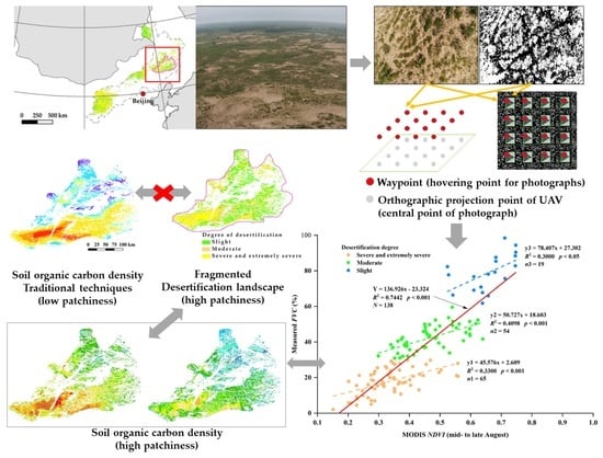
Mapping of Soil Organic Carbon Stocks Based on Aerial Photography in a Fragmented Desertification Landscape

Abstract

Northern China’s agropastoral ecotone has been a key area of desertification control for decades, and digital maps of its soil organic carbon (SOC) stocks are needed to reveal the gaps between the actual SOC levels and baseline to support land degradation neutrality (LDN) under the Sustainable Development Goals. However, reliable soil information is scarce, and accurate prediction is hindered by the fragmented landscape, which is a dominant characteristic of desertified land. To improve the patchiness identification and accuracy of SOC prediction, we conducted field surveys and collected low-altitude aerial images along the desertification degrees (severe and extremely severe, moderate, slight) in the Horqin Sandy Land. Linear regressions were performed on the relationships between the normalized difference vegetation index and the fractional vegetation cover (FVC) extracted from aerial images, and regression kriging was applied to predict SOC stocks based on the soil-forming factors (vegetation, climate, and topography). Our prediction and cross-validation showed that the fragmented structure and prediction accuracy of SOC stocks were both greatly improved for desertified land. The FVC (R²_c = 0.94) and evapotranspiration (R²_c = 0.86) had significant positive effects on SOC stocks, respectively, with indirect and direct causal relationships. Our results could provide soil information with better patchiness and accuracy to help policymakers determine the future LDN status in this fragmented desertification landscape. As drone technology becomes more available, it will fully support digital mapping of soil properties.

1. Introduction

Land cover and carbon stocks are two of the three proposed global indicators that will be used to assess land degradation neutrality (LDN) status [1,2]. LDN is an important target for terrestrial life and has been prioritized in the United Nations 2030 Agenda for Sustainable Development, with the goal of avoiding, reducing, and reversing pervasive and systemic land degradation worldwide [3,4,5,6]. This land-related target relies on an inventory of degraded land that permits a comparison with the baseline status, including the area, type, extent, degree, and causes of degradation [7]. Because of the relationship between soil organic carbon (SOC) stocks and ecosystem health, SOC has become a reasonable proxy for ecosystem resilience in the context of unsustainable use and mismanagement of land [8,9].

Land and soil degradation affects up to 30% of the world’s soils and the well-being of 3.2 billion people [6,10,11]. Thus, soil databases and digital soil mapping provide essential information within the LDN framework. The first world map of human-induced soil degradation was compiled under the UNEP-funded Global Assessment of Soil Degradation project in the late 1980s [12], and the GlobalSoilMap project followed in 2009 [13]. In China, the dataset of deserts and desertified land is one of the most widely used digital atlases since the late 1970s [14,15]. Compared with on-site observations, accurate and latest digital soil databases can provide a faster and more convincing way to describe a region’s LDN status.

Numerous advanced computational approaches [16,17] and case studies have been reported on spatial prediction, characterizing the deterministic and stochastic variation of soil properties [18,19]. These include geostatistical and hybrid techniques [20,21] and multiple regression and deep learning [16,22,23,24]. The functional relationships are established between soil properties and soil-forming factors (covariates). These are sometimes described as the SCORPAN model, with the letters representing soil, climate, organisms, relief (topography), parent material, age, and spatial position, respectively [16,25]. However, the high patchiness [7,26], as one of the most prominent features of desertified land (overgrazing and over-reclamation induced by extensive short-term farming in an agropastoral ecotone) [27,28], becomes a main obstacle to the accuracy of spatial prediction of traditional techniques. To alleviate this problem, one of the past practices is to perform labor-intensive, expensive, and time-consuming dense sampling [21,29], and other studies have focused on the fineness of resolution to characterize the differences between landscape fragments [26,30,31].

In recent decades, the potential and advantages of lightweight unmanned aerial vehicles (UAVs) in field surveys have been proven [26,32,33]. Lightweight UAVs provide an inexpensive platform for aerial photography and represent a flexible alternative to satellite imagery, thus becoming a bridge between satellite and on-site observations. Although there is no direct relationship between SOC stocks and aerial images, studies have demonstrated that the red, green, and blue (RGB) images provided by UAV-mounted sensors can be very useful for vegetation patch identification [34,35,36,37]. However, it remains unclear whether UAV-based vegetation information can improve the identification of soil patches. Northern China’s agropastoral ecotone is an ideal area for exploring the ability of UAV technology to capture the patchiness of the desertification landscape. In desertification landscapes, SOC stocks may vary with changes in vegetated and bare patches, so we hypothesized that the fractional vegetation coverage (FVC) can serve as a relevant covariate for organic carbon inputs to soils. Although this technology would have limitations under its current state of development, the results would nonetheless be sufficiently promising to justify the additional exploration of this technology. In the present study, we therefore defined the following main objectives: (1) to test the possibility of identifying patchiness of SOC stocks based on the relationship between UAV RGB images and desertification degrees; and (2) to improve the estimation of SOC stocks and quantify the causal relationships between SOC stocks and soil-forming factors in the desertification landscape.

2. Materials and Methods

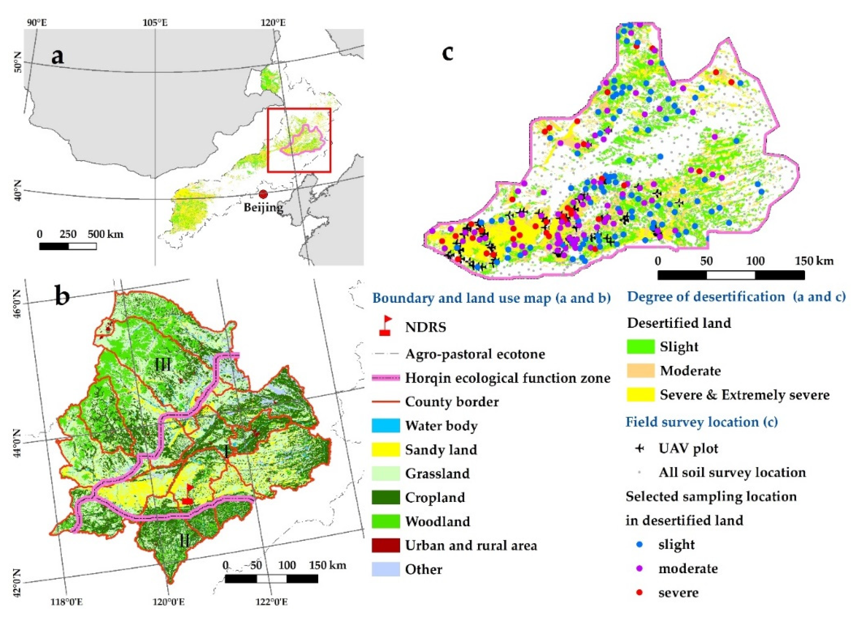
2.1. Study Area

Northern China’s agropastoral ecotone covers a total area of 73.8 × 10⁴ km², of which 37.59 × 10⁴ km² (50.9%) was desertified in 2010 [14]. The Horqin Sandy Land is situated in the southeastern part of the ecotone (Figure 1). It is a national ecological function zone that protects surrounding areas against aeolian desertification and covers 5.4 × 10⁴ km² (42°42′35″N to 44°49′48″N and 118°51′20″E to 123°42′3″E). It has a temperate continental semiarid monsoonal climate [38]. The area belongs to a drainage basin in the middle and lower reaches of the Western Liaohe River [39], whose total annual precipitation (AP) ranges from 530 mm in the southeast to 360 mm in the northwest, of which 75% fall from June to September. The mean annual temperature (MAT) ranges from 5.6 to 7.8 °C. The mean monthly temperatures change from a minimum (January) of −12.6 to −16.8 °C to a maximum (July) of 20.3 to 23.5 °C (www.resdc.cn, accessed on 6 May 2020). The elevation ranges from 88 m to 959 m asl, and rivers flow primarily from southwest to northeast. Due to severe desertification since the 1950s, the dominant zonal soils have mostly degraded under wind erosion from Kastanozems and Chernozems to Arenosols in the taxonomy of the World Reference Base for Soil Resources [40].

2.2. Desertification Classification System and UAV Flight Settings

Our sampling locations were designed according to the classification system of aeolian desertification [41,42,43,44,45], which integrated land characteristics, desertification causes, vegetation–soil system, and landscape composition.

Table 1. Classification system of aeolian desertification in northern China’s agropastoral ecotone.

Desertification Degree	Vegetation Cover (%)	Landscape Features
Extremely severe	<10	Landscape dominated by continuous mobile dunes, unproductive land with a few pioneer plant individuals (e.g., Agriophyllum squarrosum).
Severe	10–30	Mobile sand covers >50% of the area, sparse vegetation dominated by a few annual herbs and pioneer subshrubs (e.g., Artemisia halodendron).
Moderate	30–60	Mobile sand covers 25 to 50% of the area, with obvious vegetation differences between the windward and leeward slopes of dunes as a result of wind erosion and sediment deposition. soil or biological soil crust covers 30 to 80% of the area.
Slight	>60	Scattered patches of mobile sand in <25% of the area, with the original vegetation structure mostly preserved. More than 80% of the area is covered by soil or biological soil crust.

describes the classification criteria. In the present study, we set extremely severe and severe desertification as one category because their soil properties are almost similar [28].

We obtained RGB images of the UAV plots during the 2016 and 2017 growing seasons (mid- to late August) by using a Sony EXMOR Sensor mounted on a DJI Phantom 3 Professional (DJI Innovation Company Inc., Shenzheng, China). The DJI Phantom 3 Professional was a quad-rotor drone and was controlled by an automatic flight system of the FragMAP (compiled application v2016 based on Android system by Yi, Nantong, China) [46]. In the grid mode of FragMAP (Figure 2d), it defined a total of 16 waypoints at equal intervals in each 250 m × 250 m UAV plot. A 4 × 4 grid of waypoints, which formed a 200 m × 200 m square, corresponded to 16 “digital quadrats”. During operation, the UAV flew at an altitude of 20 m from the ground and took images in the order of the waypoints it passed through, with ±0.5 m vertical and 1.5 m horizontal positioning accuracy. Therefore, the digital quadrats (images), with a length-to-width ratio of 4:3, were independent (i.e., nonoverlapping), and each covered a theoretical area of about 35 m × 26 m on flat ground. The resolution of each image was 12 million pixels, and the ground sample distance was about 1 cm per pixel. The total area covered by the 16 digital quadrats was approximately 1.46 ha, which represents almost 25% of each UAV plot (Figure 2f). There was negligible geometric distortion at the edges of each image because each image was centrally projected and had a high ratio of flight height to vegetation height [34,35].

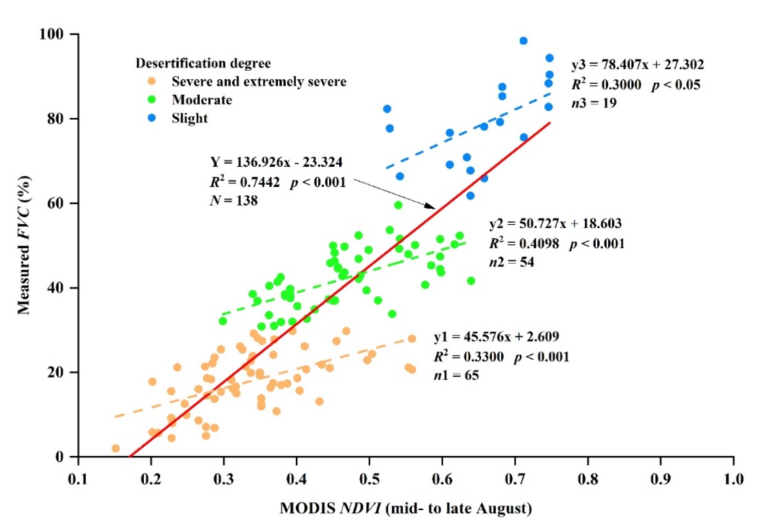
2.3. Image Postprocessing for Fractional Vegetation Coverage

In order to extract the fractional vegetation cover (FVC), the images were classified with green vegetation and bare patches using the application of FragMAP [46]. The application allows users to preview the classification results of an image and alter the results by fine-tuning the threshold for the excess green index (Figure 2e) [35]. We extracted the FVC from 2208 digital quadrats of a total of 138 UAV plots, and each plot corresponded to 1 to 2 adjacent pixels of the MODIS/Terra Vegetation Indices (MOD13Q1) at 250 m resolution [47]. The FVC of each UAV plot was represented by the average of the 16 digital quadrats (Figure 2f). Based on the average FVC, we divided the UAV plots into three categories according to the desertification classification system (Figure 2g): slight (FVC > 60%), moderate (30% < FVC ≤ 60%), and severe and extremely severe (FVC ≤ 30%).

2.4. Soil Sampling and Estimation of SOC Stocks

The data on SOC density were selected from 231 plots out of 1465 sampling locations in a soil survey [29] by our research group (Naiman Desertification Research Station, Figure 1b) conducted throughout the Horqin area. All the sampling locations for the soil survey were identified in a grid of approximately 10 km × 10 km (Figure 1c). Each location should represent a certain area (at least 500 m × 500 m), and its underlying surface features should be relatively uniform. This study focused only on desertified patches (based on the 2010 desertification map). The selected sampling locations did not include nondesertification areas (indicated by gray points in Figure 1c) such as cropland and woodland (Figure 1b). We divided the 231 locations into the three desertification categories (99 for slight desertification, 97 for moderate desertification, and 35 for severe and extremely severe desertification). The sample size was approximately proportional to the areas of each desertification category in the prediction map.

Soil samples were collected using a 2.5 cm diameter auger at a depth of 100 cm for five depth ranges (0–10 cm, 10–20 cm, 20–40 cm, 40–60 cm, and 60–100 cm). The samples were obtained from 15 randomly selected sampling points within each plot [29]. These replicated samples were mixed to prepare a single composite sample from each layer. The SOC content was measured using the K₂Cr₂O₇-H₂SO₄ oxidation method of Walkley and Black [48]. Intact soil cores were acquired at three additional sampling points, using a stainless-steel cylinder with a volume of 100 cm³ that was equipped with a soil auger. Soil cores were divided into five depth layers, which corresponded to each layer in the SOC samples. The soil cores were then oven-dried at 105 °C for 24 h to calculate the bulk density [19].

We derived the soil organic carbon density (SOCD, kg/m²) from the total SOC stock to a certain depth in the soil and expressed the value per m²:

$$SOCD=C\times Bd\times \left(1-{\delta }_{2mm}\right)\times V/1000$$

(1)

where C (%) is the SOC content; Bd (g/cm³) is the soil bulk density; V (cm³) is soil volume which is expressed as the value per m² area in the quadrat; and δ_2mm (%) is the volume fraction of gravel and other coarse material larger than 2 mm in diameter in the soil layer [49]. However, all samples were sandy soil and had no particles larger than 2 mm in diameter in the present study.

For n soil layers (1 ≤ i ≤ n), SOCD can be calculated as follows:

$$SOCD={{\displaystyle \sum }}_{i=1}^n[H_i\times B{d}_i\times (C_i/100)]$$

(2)

where H_i (cm), Bd_i (g/cm³), and C_i (g/kg) represent the thickness, bulk density, and SOC content of soil layer i, respectively. SOCD₄₀ and SOCD₁₀₀ represent SOCD in the soil profile to a depth of 40 cm (n = 3 soil layers) and 100 cm (n = 5 soil layers), respectively. We chose a depth of 40 cm for the present study because it represented the rooting zone for most of the vegetation in our study area.

2.5. Spatial Dataset Acquisition and Comparison

2.5.1. Data Sources of Land Desertification

The vector data of land desertification (2010, 1:100,000, Figure 1c) was obtained from the National Earth System Science Data Center [14]. It is fully displayed in the existing literature and atlases [41,45].

2.5.2. Vegetation and Climate Covariates

We extracted the Terra Moderate Resolution Imaging Spectroradiometer (MODIS) MOD13Q1 v061 Normalized Difference Vegetation Index (NDVI) dataset (16-day and 250 m resolution, https://lpdaac.usgs.gov/products/mod13q1v061/, accessed on 6 March 2022) and MOD16A2GF v061 Evapotranspiration (ET) dataset (8-day and 500 m resolution https://lpdaac.usgs.gov/products/mod16a2gfv061/, accessed on 6 March 2022) by an associated tool named AρρEEARS (https://lpdaacsvc.cr.usgs.gov/appeears/, accessed on 6 March 2022). We then established piecewise linear regression and general linear regression relationships between the measured FVC and the MODIS NDVI (Day 225 to Day 241 in 2016 and 2017, the UAV imaging time) of specified pixel(s) that cover each UAV plot. If a UAV plot covered parts of two or more MODIS pixels, we used the mean value of the MODIS pixels to represent the NDVI value. To account for interannual fluctuation of vegetation cover, we obtained the annual NDVI values from 2014 to 2017, which were derived from the monthly NDVI values by means of the maximum-value-composite method. We calculated the average maximum FVC during the 4 years based on the abovementioned linear regression relationships. Finally, we produced a prediction map of the desertification degrees for 2014 to 2017 based on the maximum FVC.

Spatial datasets for climate (AP and MAT time series, 1 km resolution) were obtained from the Data Center for Resources and Environmental Sciences, Chinese Academy of Sciences (www.resdc.cn, accessed on 6 May 2020). The AP, MAT, and ET were resampled to 250 m resolution, consistent with the UAV plot and MODIS NDVI. Because the influence of climate on soil formation is basically uniform on the subkilometer scale, and its variation is completely negligible [16]. Given the slow change in SOC stocks, we used the annual averages (from 2006 to 2015) of the indicators (AP, MAT, and ET) for each pixel. In addition, the yearly ET was the sum during the growing seasons from Day 113 (23 April) to Day 265 (22 September).

2.5.3. Topographic Covariates

In areas prone to aeolian desertification, topography (resampled to 250 m resolution) plays a critical role in particle transport. Thus, we accounted for the effects of slope, slope aspect (SA), and elevation, which were derived from the DEM product of the Shuttle Radar Telemetry Mission [50].

2.5.4. Digital Soil Database for Comparison

We used the soil dataset of SoilGrids250m version 2.0 [51], which is a global gridded soil information that provides soil profiles to a depth of 200 cm (https://www.isric.org/explore/soilgrids/faq-soilgrids, accessed on 16 June 2020). It was created using machine learning methods and was released by World Soil Information. We extracted SOC stock data for the first five layers (0–5 cm, 5–15 cm, 15–30 cm, 30–60 cm, and 60–100 cm).

2.6. Statistical and Prediction Methods

2.6.1. Regression Kriging and Cross-Validation

Regression kriging is a hybrid of ordinary least-squares regression and geostatistical technique, which combines the trend term $\mu \left(x\right)$ of the least-squares regression (non-geostatistical) with the kriged residual term ${\mathsf{\epsilon }}^{\prime }\left(x\right)$ from the geostatistical analysis:

$$Z\left(x\right)=\mu \left(x\right)+{\epsilon }^{\prime }\left(x\right)+{\epsilon }^{″}\left(x\right)$$

(3)

where $Z\left(x\right)$ and $\mathsf{\epsilon }″\left(x\right)$ indicate the random variable Z and the unexplained variability at location x, respectively [20]. The kriged residual term (${\epsilon }^{\prime }\left(x\right)$) indicates the variability that can not be explained by the trend term ($\mu \left(x\right)$) of the regression model. We used “Empirical Bayesian Kriging (EBK) Regression Prediction” as a hybrid interpolation method, combining the explanatory variable rasters (for $\mu \left(x\right)$, including FVC, MAT, AP, ET, elevation, slope, and SA) with EBK (for ${\epsilon }^{\prime }\left(x\right)$) for SOCD prediction and its standard error in ArcGIS Pro 2.9 (www.esri.com, accessed on 6 May 2020).

Before establishing the EBK regression model, the algorithm transforms the variable rasters into their principal components (uncorrelated with each other), which are used as explanatory variables (95% for the minimum cumulative percent of variance) in the regression model to solve the multicollinearity problem. It combines kriging and regression analysis to obtain more accurate predictions than using regression or kriging alone. Compared with other models of regression kriging, local computation is the biggest advantage of the EBK regression method. That is, the model can change itself in different regions by accounting for local effects (https://pro.arcgis.com/en/pro-app/latest/help/analysis/geostatistical-analyst/what-is-ebk-regression-prediction-.htm, accessed on 6 May 2020). In addition, it also accounts for the uncertainty of semivariogram estimation [52]. Thus, compared with the ordinary kriging (for more details, please see https://pro.arcgis.com/en/pro-app/latest/help/analysis/geostatistical-analyst/understanding-ordinary-kriging.htm, accessed on 6 May 2020), the EBK regression method has been substantially improved in all aspects.

The geostatistical wizard of ArcGIS Pro provides the leave-one-out cross-validation to determine the goodness of fit for the SOCD data and quantifies the goodness using the mean error (ME, Equation (S1)), root-mean-square error (RMSE, Equation (S2)), mean standardized error (MSE, Equation (S3)), and root-mean-square standardized error (RMSSE, Equation (S4)) (Equations (S1)–(S4) are detailed in the Supplementary Material). The leave-one-out method works by removing a single location from the dataset (1 of n) as the test set and using the remaining locations (n-1) as the training sets [52]. It is a specific case of k-fold cross-validation, where k is equal to the sample size (n). At any location in desertified land, x_i represents an array of pixel values for multiple remotely sensed covariates in the SCORPAN model [24].

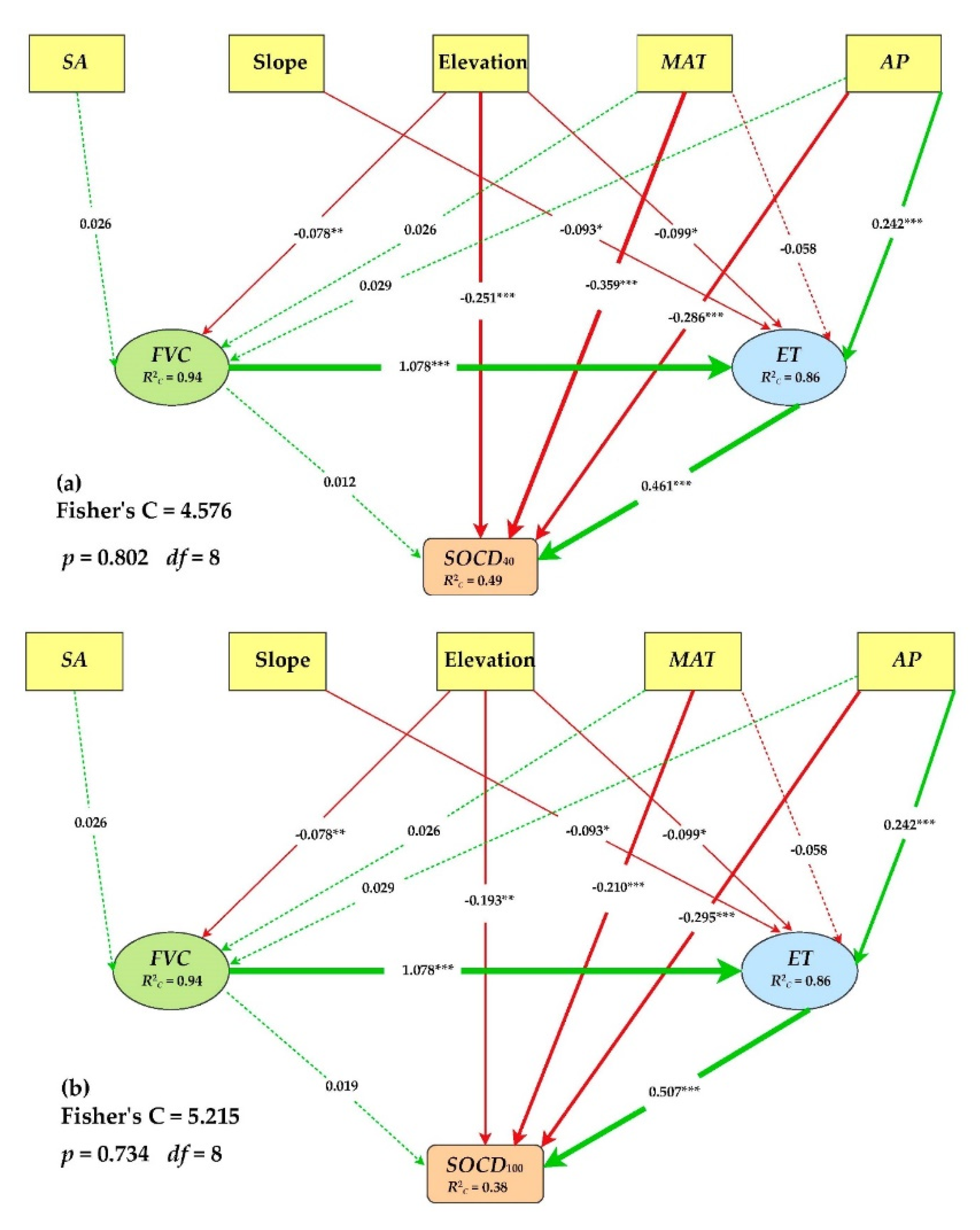
2.6.2. Structural Equation Modeling

We used structural equation modeling (SEM) [53,54] to clarify path characteristics and causal relationships (direct or indirect effects) between SOCD and the soil-forming factors and performed confirmatory factor analysis by using the R package of piecewise SEM [54]. All variables were standardized to the same dimension to account for differences in the units of measurement and magnitudes of the values. A path diagram (for SOCD₄₀ and SOCD₁₀₀, respectively) was used to represent mathematically specified causal assumptions with arrows in this statistical framework. We chose piecewise SEM with a mixed linear model (degree of desertification as a random effect) because the assumption that all observations are independent is the statistical basis for traditional SEM. Fisher’s C statistic was calculated to assess the goodness of fit of the model. When p < 0.05, it indicates that the model is missing one or more paths that contain useful information; when p > 0.05, the model represents better goodness of fit, and there are no missing paths [54].

2.6.3. Multiple Comparisons

We used Duncan’s new multiple range test (p < 0.05) to perform multiple comparisons of the measured SOC densities (SOCD) for the three desertification categories (severe and extremely severe, moderate, slight). The SOCD was log₁₀-transformed before the testing, as the raw data did not pass the Kolmogorov–Smirnov test (p < 0.05).

3. Results

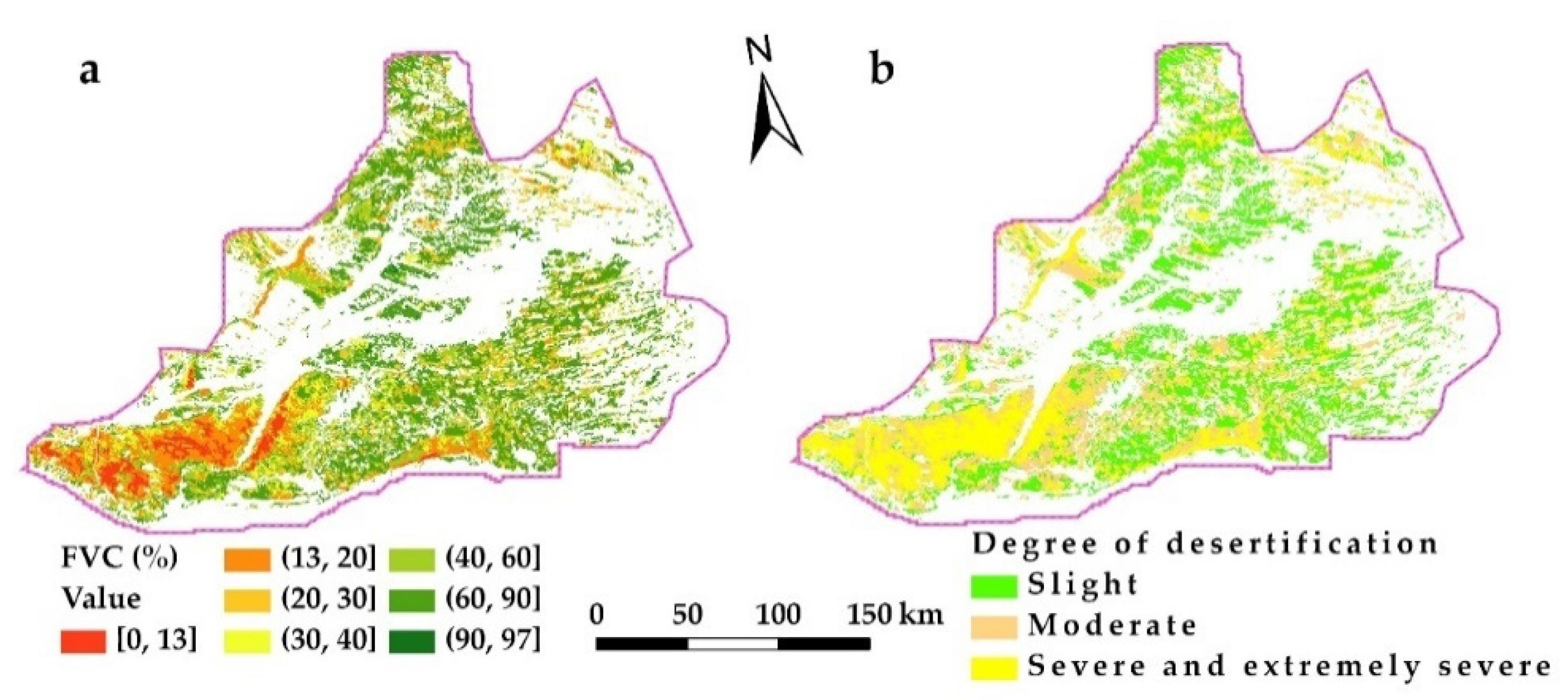
3.1. Prediction of Spatial Pattern of the Desertification Degree

Figure 3 shows statistically significant positive linear relationships between NDVI and the FVC measured by means of low-altitude aerial images for the three desertification categories. The strength of the relationship was moderate for severe and extremely severe desertification (R² = 0.3300), and moderate desertification (R² = 0.4098), and weaker for slight desertification (R² = 0.3000). For all UAV plots combined, the relationship was strong (R² = 0.7442), with a slope of 136.92.

Based on the regression models (y1, y2, and y3) in Figure 3, the spatial pattern of the average FVC from 2014 to 2017 was predicted (Figure 4). The results showed that the areas with extremely low vegetation cover were continuously distributed in the severely desertified land in the southwest, accounting for 29.2% of the Horqin Sandy Land (

Table 2. Pixel statistics of fractional vegetation cover for each desertification category.

Desertification Degree	Proportion of Area (%)	Spatial Average of FVC (%)
Severe and extremely severe	29.2	18.9
Moderate	30.4	44.0
Slight	40.4	73.6
Average		48.7

). The moderate desertification covered 30.4% of the desertified area, versus 40.4% for the slightly desertified land. The FVC averaged 73.6% for slight desertification, 44.0% for moderate desertification, and 18.9% for severe and extremely severe desertification.

3.2. Relationship between the Desertification Degree and SOCD

Figure 5 shows the results of multiple comparison of the measured SOCD₄₀ and SOCD₁₀₀ for the three desertification categories and the total. It indicates a significant (p < 0.001) SOCD decrease with the development of desertification. SOCD₄₀ and SOCD₁₀₀ decreased by 25.8% and 25.9% from slight to moderate desertification, respectively, versus decreased by 40.1% and 39.3% from moderate to severe and extremely severe desertification.

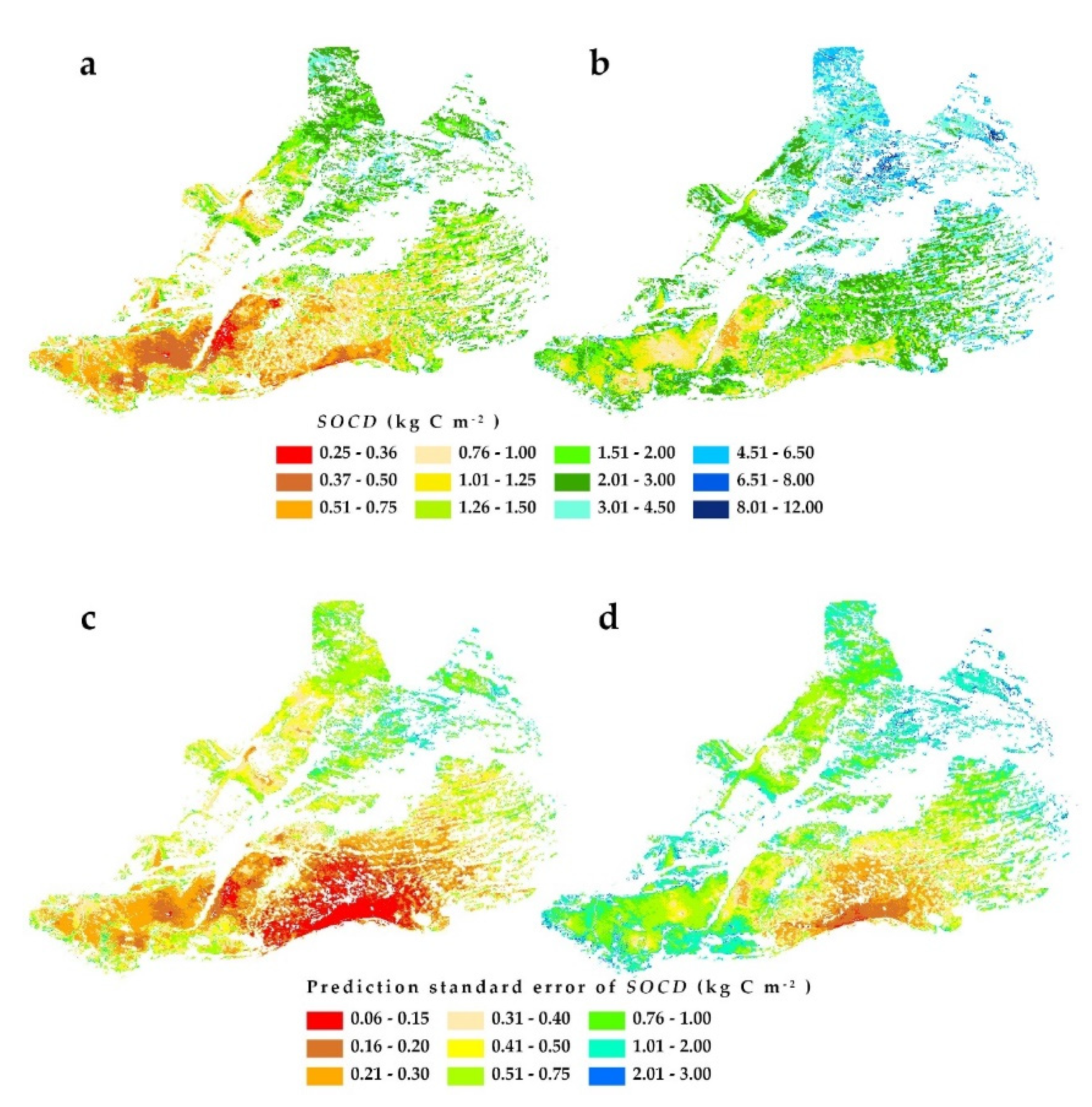
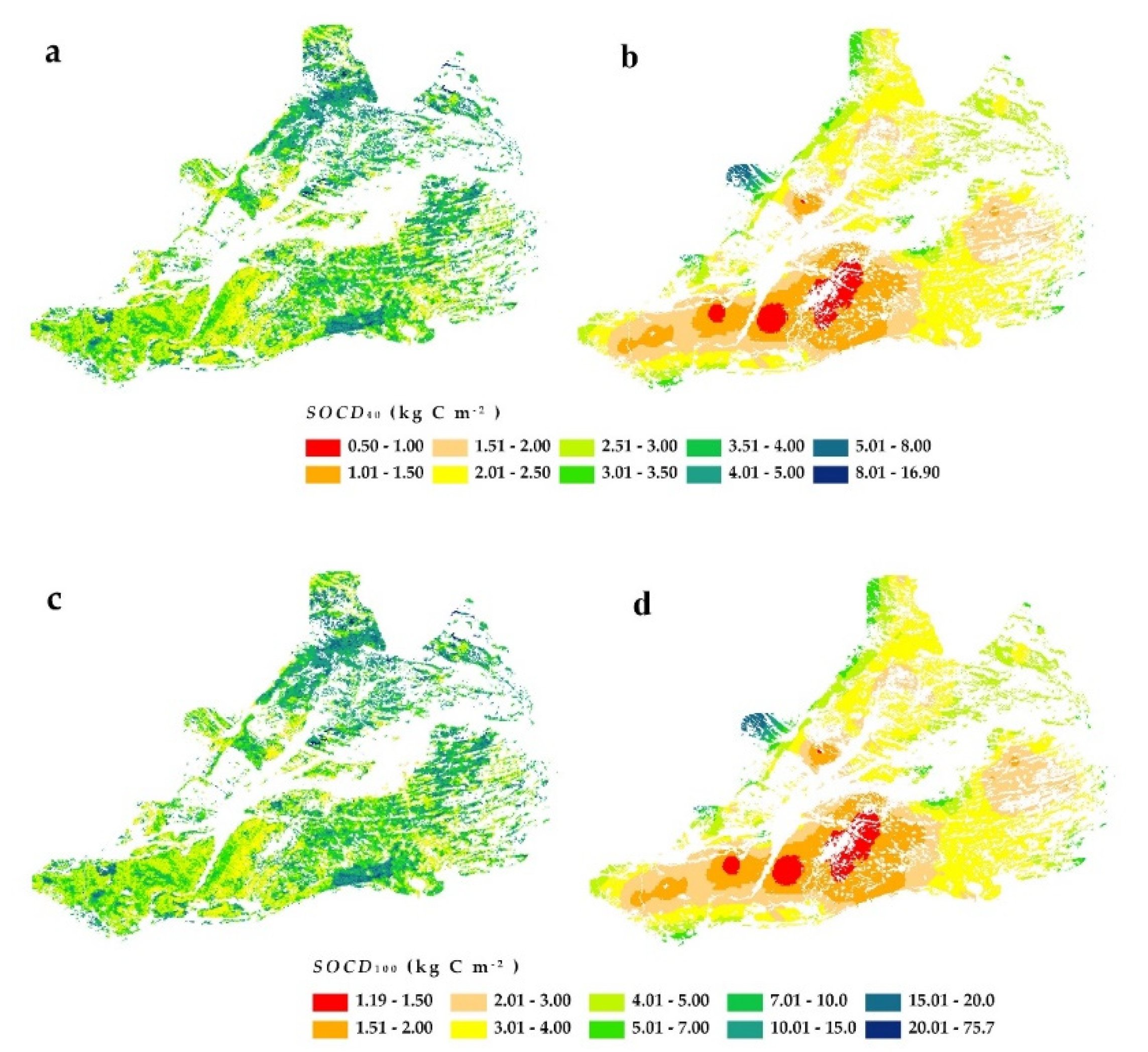
3.3. Prediction of Spatial Patterns of SOCD Based on Soil-forming Factors

Empirical Bayesian kriging (EBK) regression prediction was used to predict SOCD based on the soil-forming factors (FVC, MAT, AP, ET, slope, SA, and elevation). SOCD₄₀ (Figure 6a) averaged 1.86 kg C m⁻² (slight desertification), 1.26 kg C m⁻² (moderate desertification) and 0.87 kg C m⁻² (severe and extremely severe desertification), with the standard errors of prediction (Figure 6c) averaged 0.53, 0.41 and 0.32 kg C m⁻², respectively. SOCD₁₀₀ (Figure 6b) averaged 3.63 kg C m⁻² (slight desertification), 2.49 kg C m⁻² (moderate desertification) and 1.73 kg C m⁻² (severe and extremely severe desertification), with the standard errors (Figure 6d) averaged 0.97, 0.83, and 0.66 kg C m⁻², respectively.

The leave-one-out cross-validation method was used to evaluate the differences between the measured and predicted SOCD values, including the results of EBK regression, EBK, and ordinary kriging (

Table 3. Results of leave-one-out cross-validation for SOCD prediction. Abbreviations: FVC, fractional vegetation cover; AP, annual precipitation; MAT, mean annual temperature; ET, evapotranspiration; SA, slope aspect; ME, mean error; RMSE, root-mean-square error; MSE, mean standardized error; RMSSE, root-mean-square standardized error.

Independent Variables	Soil Layer	ME	RMSE	MSE	RMSSE
FVC, MAT, AP, ET, slope, SA, and Elevation (EBK Regression)	0–40 cm	−0.009	0.841	−0.012	0.946
	0–100 cm	0.032	1.940	0.008	0.964
None (Empirical Bayesian Kriging)	0–40 cm	−0.007	0.988	−0.004	0.927
	0–100 cm	−0.007	2.172	−0.003	0.976
None (Ordinary Kriging)	0–40 cm	0.338	1.154	0.081	0.472
	0–100 cm	0.411	2.329	0.043	0.702

). Our prediction accuracy of SOCD₄₀ was higher than that of SOCD₁₀₀, with an RMSE of 0.841 and 1.940 kg C m⁻². The results of EBK regression and EBK were valid and robust, as the RMSSE was closer to 1 in each case. In the EBK method, all the soil-forming factors were excluded from the regression, and the RMSE increased by 17.5% (SOCD₄₀) and 12.0% (SOCD₁₀₀), respectively, while the RMSE of the ordinary kriging method was much higher than that of the other two methods.

4. Discussion

4.1. Patchiness Identification and Relationships between SOCD and Soil-Forming Factors

Aeolian desertification has long-term effects on SOC dynamics [42], as organic matter input is considered an important measure to maintain and enhance SOC [55,56]. The magnitude and direction (positive and negative processes) of desertification are strongly related to changes in vegetation cover and soil texture [27,57], which further affect leaf area index, evapotranspiration, productivity, and litter input [57,58,59,60]. SEMs (p > 0.05) were performed to examine the causal relationships between the soil-forming factors and SOCD (Figure 7). Taking the degree of desertification (Figure 4b) as a random effect, FVC had an extremely weak direct effect on SOCD₄₀, whereas the greatest and indirect positive effect mediated through ET (1.078 × 0.461 = 0.497). Spatially, AP (−0.286), MAT (−0.359), and Elevation (−0.251) showed significant and direct effects on SOCD₄₀ (Figure 7a), and AP had a positive and indirect effect on SOCD₄₀ through ET (0.242 × 0.461 = 0.112). Overall, the path coefficients of SOCD₁₀₀ retained the same signs as SOCD₄₀ (Figure 7a,b).

FVC and ET, the most important predictors, connect the plant–organic matter–soil system through photosynthesis processes [61,62]. On the dune tops and windward sides, it always has lower shielding by plants (−0.078). Organic matter is more vulnerable to wind erosion due to the rapid migration of fine particles (coarsening of soil texture) in loose soils [27]. In addition, suitable temperature [59,63] and moisture [64,65] can promote the decomposition of organic matter by microbial communities, while infiltrated rainwater has a leaching effect on the limited organic matter. This may be the reason why increasing temperature and moisture accelerate the loss of organic matter. On the other hand, the interdune lowlands are highly correlated with the distribution of moisture and nutrients [66], which is relatively favorable for vegetation growth. The rainfall, therefore, has a positive indirect effect on SOCD through vegetation evapotranspiration (0.242).

The FVC, coupled with biological soil crusts, is the most direct quantitative indicator that delivers desertification information [42,67,68]. However, the traditional measurements of the FVC have always been faced with a dilemma: observations from different studies are too different to follow the unified standard based on the ocular estimation method, and lens coverage is too small to fully represent the area of interest by the photographic method [34,69]. The use of UAV images combines the advantages of the traditional quadrat-based approach and digital photos to address both problems [34,35,46]. The spatial extent of field observations can be extended from the level of the traditional 1 m² quadrat to the pixel level of satellite data. Therefore, the degree of desertification can be defined more accurately, which provides a more convincing basis for the relationship between SOCD and the degree of desertification.

4.2. Comparisons of Patchiness and Accuracy for SOCD Mapping

SOCD tends to be low in wind-eroded soils. In China’s agropastoral ecotone, SOCD is highly consistent with the degree of aeolian desertification [27,57]. We compared the patchiness and accuracy of SOCD mapping from this study with the data from two sources (SoilGrids250m and previous research). Our SOCD predictions depend on the field survey with locations, the effects of soil-forming factors, and the degree of desertification. The spatial pattern of SOCD revealed the fragmented structure of the desertification landscape (Figure 6).

In the same area, SOCD₄₀ from the SoilGrids250m data [22] averaged 3.48, 3.45, and 3.52 kg C m⁻² (Figure 8a and Table S1) under slight, moderate, and severe and extremely severe desertification, respectively, versus SOCD₁₀₀ values of 10.17, 10.39, and 10.56 kg C m⁻² (Figure 8c), while the results of traditional geostatistical method averaged 2.07 and 3.89 kg C m⁻² to a depth of 40 cm [21] and 100 cm [29] under slight desertification, respectively, versus 1.90 and 2.94 kg C m⁻² under severe and extremely severe desertification (Figure 8b,d and Table S1). The fragmented structure of the SoilGrids250m data was preserved much better than that of the geostatistical method [21,29]. However, the values of SOCD_SoilGrid250m for the three desertification categories were considerably higher than the results of this study and previous geostatistical research (Table S1).

It suggested that SOCD_SoilGrid250m was greatly overestimated when compared with our measured values (Figure 5). Essentially, SOCD_SoilGrid250m showed an inverse gradient or no gradient with the degree of desertification, which clearly contradicts our predictions and previous studies in the Horqin Sandy Land [27,67]. The accuracy of SOCD_SoilGrid250m, therefore, needs to be greatly improved for the desertification landscape, such as the Horqin Sandy Land. On the other hand, the traditional geostatistical methods have problems in dealing with patchiness. The algorithm of EBK has an obvious advantage, and accounting for the soil-forming factors can improve the prediction accuracy. Our study partially addresses both problems and, therefore, merits additional study in other desertified areas to confirm its ability to be generalized and its validity under different conditions.

5. Conclusions

We introduced the desertification classification system into the prediction of SOC stocks based on soil-forming factors. The high patchiness of the soil in the desertified area was identified based on the relationship between the FVC and desertification degree. Our results greatly improved the prediction accuracy of SOC density. The prediction demonstrated the potential of using UAVs to survey SOC stocks and partially addressed the mismatch between quadrat representation and survey scope encountered in previous methods. Among the soil-forming factors we investigated, ET and FVC played positive and critical roles in the prediction, directly and indirectly, significantly affecting SOC stocks along the desertification gradient. Looking into the future, UAV sensors will become an important platform for predicting soil properties in fragmented landscapes.

References

1. Cowie, A.L.; Orr, B.J.; Castillo Sanchez, V.M.; Chasek, P.; Crossman, N.D.; Erlewein, A.; Louwagie, G.; Maron, M.; Metternicht, G.I.; Minelli, S.; et al. Land in balance: The scientific conceptual framework for Land Degradation Neutrality. Environ. Sci. Policy 2018, 79, 25–35. [Google Scholar] [CrossRef]
2. Chasek, P.; Akhtar-Schuster, M.; Orr, B.J.; Luise, A.; Rakoto Ratsimba, H.; Safriel, U. Land degradation neutrality: The science-policy interface from the UNCCD to national implementation. Environ. Sci. Policy 2019, 92, 182–190. [Google Scholar] [CrossRef]
3. UNCCD. Report of the Conference of the Parties on Its Twelfth Session; Part Two; Action Taken: Ankara, Turkey, 2015. [Google Scholar]
4. UN. Transforming Our World: The 2030 Agenda for Sustainable Development. Available online: https://sdgs.un.org/2030agenda (accessed on 6 June 2019).
5. Kust, G.; Andreeva, O.; Cowie, A. Land Degradation Neutrality: Concept development, practical applications and assessment. J. Environ. Manag. 2017, 195, 16–24. [Google Scholar] [CrossRef] [PubMed]
6. IPBES. The IPBES Assessment Report on Land Degradation and Restoration; Montanarella, L., Scholes, R., Brainich, A., Eds.; Secretariat of the Intergovernmental Science-Policy Platform on Biodiversity and Ecosystem Services: Bonn, Germany, 2018. [Google Scholar]
7. Gibbs, H.K.; Salmon, J.M. Mapping the world’s degraded lands. Appl. Geography. 2015, 57, 12–21. [Google Scholar] [CrossRef]
8. Keesstra, S.D.; Bouma, J.; Wallinga, J.; Tittonell, P.; Smith, P.; Cerdà, A.; Montanarella, L.; Quinton, J.N.; Pachepsky, Y.; Van, D.P.W.H.; et al. The significance of soils and soil science towards realization of the United Nations Sustainable Development Goals. Soil 2016, 2, 111–128. [Google Scholar] [CrossRef] [Green Version]
9. Chappell, A.; Webb, N.P.; Leys, J.F.; Waters, C.M.; Orgill, S.; Eyres, M.J. Minimising soil organic carbon erosion by wind is critical for land degradation neutrality. Environ. Sci. Policy 2019, 93, 43–52. [Google Scholar] [CrossRef]
10. Bouma, J. How to communicate soil expertise more effectively in the information age when aiming at the UN Sustainable Development Goals. Soil Use Manag. 2019, 35, 32–38. [Google Scholar] [CrossRef] [Green Version]
11. FAO; ITP. Status of the World’s Soil Resources (SWSR)—Technical Summary; Food and Agriculture Organization of the United Nations and Intergovernmental Technical Panel on Soils: Rome, Italy, 2015. [Google Scholar]
12. Oldeman, L.R.; Hakkeling, R.T.A.; Sombroek, W.G. World Map of the Status of Human-Induced Soil Degradation: An explanatory Note, rev. ed.; UNEP and ISRIC: Wageningen, Netherlands, 1991. [Google Scholar]
13. Arrouays, D.; Grundy, M.G.; Hartemink, A.E.; Hempel, J.W.; Heuvelink, G.B.M.; Hong, S.Y.; Lagacherie, P.; Lelyk, G.; McBratney, A.B.; McKenzie, N.J.; et al. Chapter Three-GlobalSoilMap: Toward a Fine-Resolution Global Grid of Soil Properties. In Advances in Agronomy; Sparks, D.L., Ed.; Academic Press: Cambridge, MA, USA, 2014; Volume 125, pp. 93–134. [Google Scholar]
14. Yan, C. Desert (Sand) Distribution Dataset (1 km) in China. National Earth System Science Data Center; National Science & Technology Infrastructure of China. Available online: http://www.geodata.cn (accessed on 11 May 2020).
15. Yan, C.; Wang, J. 1:100000 Desert (Sand) Distribution Dataset in China. National Cryosphere Desert Data Center. Available online: http://www.ncdc.ac.cn (accessed on 6 May 2020).
16. Zhu, A.X.; Yang, L.; Fan, N.; Zeng, C.; Zhang, G. The review and outlook of digital soil mapping. Prog. Geography. 2018, 37, 66–78. [Google Scholar]
17. Zhang, Y.; Guo, L.; Chen, Y.; Shi, T.; Luo, M.; Ju, Q.; Zhang, H.; Wang, S. Prediction of Soil Organic Carbon based on Landsat 8 Monthly NDVI Data for the Jianghan Plain in Hubei Province, China. Remote Sens. 2019, 11, 1683. [Google Scholar] [CrossRef] [Green Version]
18. Wang, X.; Li, Y.; Gong, X.; Niu, Y.; Chen, Y.; Shi, X.; Li, W.; Liu, J. Changes of soil organic carbon stocks from the 1980s to 2018 in northern China’s agro-pastoral ecotone. Catena 2020, 194, 104722. [Google Scholar] [CrossRef]
19. Li, Y.; Wang, X.; Chen, Y.; Luo, Y.; Lian, J.; Niu, Y.; Gong, X.; Yang, H.; Yu, P. Changes in surface soil organic carbon in semiarid degraded Horqin Grassland of northeastern China between the 1980s and the 2010s. Catena 2019, 174, 217–226. [Google Scholar] [CrossRef]
20. Keskin, H.; Grunwald, S. Regression kriging as a workhorse in the digital soil mapper’s toolbox. Geoderma 2018, 326, 22–41. [Google Scholar] [CrossRef]
21. Wang, X.; Li, Y.; Gong, X.; Niu, Y.; Chen, Y.; Shi, X.; Li, W. Storage, pattern and driving factors of soil organic carbon in an ecologically fragile zone of northern China. Geoderma 2019, 343, 155–165. [Google Scholar] [CrossRef]
22. Hengl, T.; Mendes, D.J.J.; Heuvelink, G.B.; Ruiperez, G.M.; Kilibarda, M.; Blagotić, A.; Shangguan, W.; Wright, M.N.; Geng, X.; Bauer-Marschallinger, B. SoilGrids250m: Global gridded soil information based on machine learning. PLoS ONE 2017, 12, e169748. [Google Scholar] [CrossRef] [PubMed] [Green Version]
23. Zhang, H.; Wu, P.; Yin, A.; Yang, X.; Zhang, M.; Gao, C. Prediction of soil organic carbon in an intensively managed reclamation zone of eastern China: A comparison of multiple linear regressions and the random forest model. Sci. Total Environ. 2017, 592, 704–713. [Google Scholar] [CrossRef]
24. Padarian, J.; Minasny, B.; McBratney, A.B. Using deep learning for digital soil mapping. Soil 2019, 5, 79–89. [Google Scholar] [CrossRef] [Green Version]
25. McBratney, A.B.; Mendonca Santos, M.L.; Minasny, B. On digital soil mapping. Geoderma 2003, 117, 3–52. [Google Scholar] [CrossRef]
26. Qin, Y.; Yi, S.; Ding, Y.; Xu, G.; Chen, J.; Wang, Z. Effects of small-scale patchiness of alpine grassland on ecosystem carbon and nitrogen accumulation and estimation in northeastern Qinghai-Tibetan Plateau. Geoderma 2018, 318, 52–63. [Google Scholar] [CrossRef]
27. Zhao, H.L.; He, Y.H.; Zhou, R.L.; Su, Y.Z.; Li, Y.Q.; Drake, S. Effects of desertification on soil organic C and N content in sandy farmland and grassland of Inner Mongolia. Catena 2009, 3, 187–191. [Google Scholar] [CrossRef]
28. Li, Y.; Han, J.; Wang, S.; Brandle, J.; Lian, J.; Luo, Y.; Zhang, F. Soil organic carbon and total nitrogen storage under different land uses in the Naiman Banner, a semiarid degraded region of northern China. Can. J. Soil Sci. 2014, 94, 9–20. [Google Scholar] [CrossRef]
29. Li, Y.; Wang, X.; Niu, Y.; Jie, L.; Luo, Y.; Chen, Y.; Gong, X.; Yang, H.; Yu, P. Spatial distribution of soil organic carbon in the ecologically fragile Horqin Grassland of northeastern China. Geoderma 2018, 325, 102–109. [Google Scholar] [CrossRef]
30. Law, B.E.; Hudiburg, T.W.; Berner, L.T.; Kent, J.J.; Buotte, P.C.; Harmon, M.E. Land Use Strategies to Mitigate Climate Change in Carbon Dense Temperate Forests. Proc. Natl. Acad. Sci. USA 2018, 115, 3663–3668. [Google Scholar] [CrossRef] [PubMed] [Green Version]
31. Ballabio, C.; Fava, F.; Rosenmund, A. A plant ecology approach to digital soil mapping, improving the prediction of soil organic carbon content in alpine grasslands. Geoderma 2012, 187, 102–116. [Google Scholar] [CrossRef]
32. Laliberte, A.S.; Rango, A. Texture and Scale in object-based Analysis of Subdecimeter Resolution Unmanned Aerial Vehicle (UAV) Imagery. IEEE T. Geosci. Remote 2009, 47, 761–770. [Google Scholar] [CrossRef] [Green Version]
33. Hao, M.; Zhao, W.; Qin, L.; Mao, P.; Qiu, X.; Xu, L.; Xiong, Y.J.; Ran, Y.; Qiu, G. A methodology to determine the optimal quadrat size for desert vegetation surveying based on unmanned aerial vehicle (UAV) RGB photography. Int. J. Remote Sens. 2021, 42, 84–105. [Google Scholar] [CrossRef]
34. Chen, J.; Yi, S.; Qin, Y.; Wang, X. Improving estimates of fractional vegetation cover based on UAV in alpine grassland on the Qinghai–Tibetan Plateau. Int. J. Remote Sens. 2016, 37, 1922–1936. [Google Scholar] [CrossRef]
35. Yi, S.; Chen, J.; Qin, Y.; Xu, G. The burying and grazing effects of plateau pika on alpine grassland are small: A pilot study in a semiarid basin on the Qinghai-Tibet Plateau. Biogeosciences 2016, 13, 6273–6284. [Google Scholar] [CrossRef] [Green Version]
36. Tang, L.; He, M.; Li, X. Verification of Fractional Vegetation Coverage and NDVI of Desert Vegetation via UAVRS Technology. Remote Sens. 2020, 12, 1742. [Google Scholar] [CrossRef]
37. Mao, P.; Qin, L.; Hao, M.; Zhao, W.; Luo, J.; Qiu, X.; Xu, L.; Xiong, Y.; Ran, Y.; Yan, C.; et al. An improved approach to estimate above-ground volume and biomass of desert shrub communities based on UAV RGB images. Ecol. Indic. 2021, 125, 107494. [Google Scholar] [CrossRef]
38. Liu, X.M.; Zhao, H.L.; Zhao, A.F. Wind-Sandy Environment and Vegetation in the Horqin Sandy Land; Science Press: Beijing, China, 1996. (In Chinese) [Google Scholar]
39. Lian, J.; Zhao, X.; Li, X.; Zhang, T.; Wang, S.; Luo, Y.; Zhu, Y.; Feng, J. Detecting Sustainability of Desertification Reversion: Vegetation Trend Analysis in Part of the Agro-Pastoral Transitional Zone in Inner Mongolia, China. Sustainability 2017, 9, 211. [Google Scholar] [CrossRef] [Green Version]
40. IUSS Working Group WRB. World Reference Base for Soil Resources 2006—A Framework for International Classification, Correlation and Communication; Food and Agriculture Organization of the United Nations: Rome, Italy, 2006; Volume 103. [Google Scholar]
41. Wang, T. Atlas of Sandy Desert and Aeolian Desertification in Northern China; Science Press: Beijing, China, 2014. (In Chinese) [Google Scholar]
42. Zhao, H.L.; Zhao, R.L.; Zhao, X.Y.; Zhang, T.H. Ground Discriminance on Positive and Negative Processes of Land Desertification in Horqin Sand Land. J. Desert Res. 2008, 28, 8–15. (In Chinese) [Google Scholar]
43. Zhao, H.L.; Zhao, X.Y.; Zhang, T.H.; Wu, W.; Su, Y.Z.; Zhou, R.L.; Wang, H.O. Desertification Processes and Its Restoration Mechanisms in the Horqin Sand Land; Ocean Press: Beijing, China, 2003. [Google Scholar]
44. Zhu, Z.; Liu, S. The Concept of Desertification and the Differentiation of Its Development. J. Desert Res. 1984, 4, 2–8. (In Chinese) [Google Scholar]
45. Duan, H.C.; Tao, W.; Xian, X.; Liu, S.L.; Jian, G. Dynamics of aeolian desertification and its driving forces in the Horqin Sandy Land, Northern China. Environ. Monit. Assess. 2014, 186, 6083–6096. [Google Scholar] [CrossRef]
46. Yi, S. FragMAP: A tool for long-term and cooperative monitoring and analysis of small-scale habitat fragmentation using an unmanned aerial vehicle. Int. J. Remote Sens. 2017, 38, 2686–2697. [Google Scholar] [CrossRef]
47. Didan, K. MOD13Q1 MODIS/Terra Vegetation Indices 16-Day L3 Global 250 m SIN Grid V061. NASA EOSDIS LP DAAC. 2015. Available online: https://lpdaac.usgs.gov/products/mod13q1v061/ (accessed on 6 March 2022).
48. Nelson, D.W.; Sommers, L.E. Total carbon, organic carbon and organic matter. In Methods of Soil Analysis Part 3: Chemical Methods; Sparks, D.L., Page, A.L., Helmke, P.A., Loeppert, R.H., Soltanpour, P.N., Tabatabai, M.A., Johnston, C.T., Sumner, M.E., Eds.; American Society of Agronomy & Soil Science Society of America: Madison, WI, USA, 1996; pp. 961–1010. [Google Scholar]
49. Pouyat, R.; Groffman, P.; Yesilonis, I.; Hernandez, L. Soil carbon pools and fluxes in urban ecosystems. Environ. Pollut. 2002, 116, S107–S118. [Google Scholar] [CrossRef]
50. EROS Center. Digital Elevation-Shuttle Radar Topography Mission (SRTM) 3 Arc-Second Global; USGS. Available online: https://www.usgs.gov/centers/eros/science/usgs-eros-archive-digital-elevation-shuttle-radar-topography-mission-srtm (accessed on 11 May 2020).
51. Poggio, L.; De Sousa, L.; Batjes, N.; Heuvelink, G.; Kempen, B.; Ribeiro, E.; Rossiter, D. SoilGrids 2.0: Producing soil information for the globe with quantified spatial uncertainty. Soil 2021, 7, 217–240. [Google Scholar] [CrossRef]
52. ESRI Inc. ArcGIS Pro Help; ESRI Inc.: Redlands, CA, USA, 2020. [Google Scholar]
53. Grace, J.B.; Anderson, T.M.; Seabloom, E.W.; Borer, E.T.; Adler, P.B.; Harpole, W.S.; Hautier, Y.; Hillebrand, H.; Lind, E.M.; Pärtel, M.; et al. Integrative modelling reveals mechanisms linking productivity and plant species richness. Nature 2016, 529, 390–393. [Google Scholar] [CrossRef] [PubMed]
54. Lefcheck, J.S. piecewiseSEM: Piecewise structural equation modelling in r for ecology, evolution, and systematics. Methods Ecol. Evol. 2016, 7, 573–579. [Google Scholar] [CrossRef]
55. Zdruli, P.; Lal, R.; Cherlet, M.; Kapur, S. New World Atlas of Desertification and Issues of Carbon Sequestration, Organic Carbon Stocks, Nutrient Depletion and Implications for Food Security. In Carbon Management, Technologies, and Trends in Mediterranean Ecosystems; Erşahin, S., Kapur, S., Akça, E., Namlı, A., Erdoğan, H.E., Eds.; Springer: Berlin/Heidelberg, Germany, 2017; pp. 13–25. [Google Scholar]
56. Lal, R. Soil management and restoration for C sequestration to mitigate the accelerated greenhouse effect. Prog. Environ. Sci. 1999, 1, 307–326. [Google Scholar]
57. Li, Y.; Brandle, J.; Awada, T.; Chen, Y.; Han, J.; Zhang, F.; Luo, Y. Accumulation of carbon and nitrogen in the plant—soil system after afforestation of active sand dunes in China’s Horqin Sandy Land. Agric. Ecosyst. Environ. 2013, 177, 75–84. [Google Scholar] [CrossRef]
58. Tang, Z.; An, H.; Deng, L.; Wang, Y.; Zhu, G.; Shangguan, Z. Effect of desertification on productivity in a desert steppe. Sci. Rep. 2016, 6, 27839. [Google Scholar] [CrossRef] [PubMed]
59. Kirschbaum, M.U.F. The temperature dependence of soil organic matter decomposition, and the effect of global warming on soil organic C storage. Soil Biol. Biochem. 1995, 27, 753–760. [Google Scholar] [CrossRef]
60. Ma, X.; Zhu, J.; Yan, W.; Zhao, C. Projections of desertification trends in Central Asia under global warming scenarios. Sci. Total Environ. 2021, 781, 146777. [Google Scholar] [CrossRef] [PubMed]
61. Brown, S.M.; Petrone, R.M.; Mendoza, C.; Devito, K.J. Surface vegetation controls on evapotranspiration from a sub-humid Western Boreal Plain wetland. Hydrol. Process. 2010, 24, 1072–1085. [Google Scholar] [CrossRef]
62. Jin, Z.; Liang, W.; Yang, Y.; Zhang, W.; Yan, J.; Chen, X.; Li, S.; Mo, X. Separating vegetation greening and climate change controls on evapotranspiration trend over the Loess Plateau. Sci. Rep. 2017, 7, 8191. [Google Scholar] [CrossRef]
63. Conant, R.T.; Ryan, M.; Ågren, G.I.; Birge, H.E.; Davidson, E.A.; Eliasson, P.E.; Evans, S.E.; Frey, S.D.; Giardina, C.P.; Hopkins, F.M.; et al. Temperature and soil organic matter decomposition rates-synthesis of current knowledge and a way forward. Glob. Chang. Biol. 2011, 17, 3392–3404. [Google Scholar] [CrossRef]
64. Huang, W.; Hall, S.J. Elevated moisture stimulates carbon loss from mineral soils by releasing protected organic matter. Nat. Commun. 2017, 8, 1774. [Google Scholar] [CrossRef]
65. Zhou, Y.; Li, X.; Gao, Y.; He, M.; Wang, M.; Wang, Y.; Zhao, L.; Li, Y. Carbon fluxes response of an artificial sand-binding vegetation system to rainfall variation during the growing season in the Tengger Desert. J. Environ. Manag. 2020, 266, 110556. [Google Scholar] [CrossRef]
66. Zuo, X.; Zhao, X.; Zhao, H.; Guo, Y.; Zhang, T.; Cui, J. Spatial pattern and heterogeneity of soil organic carbon and nitrogen in sand dunes related to vegetation change and geomorphic position in Horqin Sandy Land, Northern China. Environ. Monit. Assess. 2010, 164, 29–42. [Google Scholar] [CrossRef]
67. Zhao, H.L.; Yi, X.Y.; Zhou, R.L.; Zhao, X.Y.; Zhang, T.H.; Drake, S. Wind erosion and sand accumulation effects on soil properties in Horqin Sandy Farmland, Inner Mongolia. Catena 2006, 65, 71–79. [Google Scholar] [CrossRef]
68. Zhu, Z.; Liu, S. Desertification and Its Control in China; Science Press: Beijing, China, 1989. (In Chinese) [Google Scholar]
69. Marcial-Pablo, M.D.J.; Gonzalez-Sanchez, A.; Jimenez-Jimenez, S.I.; Ontiveros-Capurata, R.E.; Ojeda-Bustamante, W. Esti-mation of vegetation fraction using RGB and multispectral images from UAV. Int. J. Remote Sens. 2019, 40, 420–438. [Google Scholar] [CrossRef]
Figure 1. Study area and sampling locations. (a) The Horqin Sandy Land is in the southeastern part of northern China’s agropastoral ecotone. (b) Land use map and administrative division of the Horqin area at a county level in 2015: (I) Horqin ecological function zone for desertification control; (II) the source region of the subcatchment of the Liaohe River; and (III) the Greater Khingan Mountains; NDRS, Naiman Desertification Research Station. (c) Locations of the soil samples and UAV plots within desertification map in 2010.
Remotesensing 14 02829 g001
Figure 2. Flowchart of UAV flight settings, fractional vegetation cover (FVC) extraction, and prediction. (a) Fragmented desertification landscapes. (b) Soil organic carbon density predicted by traditional geostatistical method is low in patchiness. (c) Desertification landscape is high in patchiness. (d) Schematic diagram of UAV waypoint distribution from top and side views. (e) Example of black and white image extracted from one RGB image to capture vegetation (white) and bare area (black). (f) Covered area of the 16 “digital quadrats” in a UAV plot. (g) Regional FVC prediction based on piecewise linear relationship between FVC and NDVI.
Remotesensing 14 02829 g002
Figure 3. Relationship between the MODIS normalized difference vegetation index (NDVI) and the fractional vegetation cover (FVC; 0 ≤ FVC ≤ 100) for the three desertification categories (for severe and extremely severe desertification, n1 = 65; for moderate desertification, n2 = 54; for slight desertification, n3 = 19). The red regression line represents the NDVIFVC relationship for all UAV plots combined (N = 138). Each point represents the average FVC from 16 images located in one or adjacent NDVI pixels.
Remotesensing 14 02829 g003
Figure 4. Spatial pattern of predicted average fractional vegetation cover (FVC) and desertified patches from 2014 to 2017: (a) predicted FVC using the regression models for each desertification category (Figure 3); (b) predicted desertification degrees based on FVC.
Remotesensing 14 02829 g004
Figure 5. Change in the measured soil organic carbon density (SOCD). Box-whisker plot shows the mean (square), median (solid line) in the boxes, and the 5th and 95th percentiles on the whiskers. The statistical significances are marked with lowercase letters for SOCD40 and capital letters for SOCD100 (p < 0.001).
Remotesensing 14 02829 g005
Figure 6. Spatial pattern of the predicted soil organic carbon density (SOCD) in the Horqin Sandy Land: (a) prediction of SOCD40 (SOCD to a depth of 40 cm); (b) prediction of SOCD100 (SOCD to a depth of 100 cm); (c) prediction standard error for SOCD40; (d) prediction standard error for SOCD100.
Remotesensing 14 02829 g006
Figure 7. Results of piecewise structural equation model for the causal relationships between soil organic carbon density (SOCD) and soil-forming factors: (a) SOCD40, SOCD to a depth of 40 cm; (b) SOCD100, SOCD to a depth of 100 cm. The green and red solid arrows, respectively, denote positive and negative unidirectional relationships that significant at p < 0.05 *, p < 0.01 **, and p < 0.001 ***, and dashed arrows nonsignificant paths (p > 0.05). The magnitude of the standardized regression coefficients was indicated by the thickness of arrows. R2c was conditional R2 that based on the variance of random (desertification degree) and fixed effects. Abbreviations: FVC, fractional vegetation cover; ET, evapotranspiration; AP, annual precipitation; MAT, mean annual temperature; SA, slope aspect.
Remotesensing 14 02829 g007
Figure 8. Spatial pattern of the predicted soil organic carbon density (SOCD). Data were obtained from the SoilGrids250m product for (a) SOCD40 (SOCD to a depth of 40 cm) and (c) SOCD100 (SOCD to a depth of 100 cm). Data were obtained from previous geostatistical research: (b) SOCD40 [21] and (d) SOCD100 [29]. The data from SoilGrids250m (metric ton ha−1) and Wang et al., (2019) were standardize to permit comparisons at 0–40 cm with our result: SOCD40(SoilGrid250m) = (SOCD0–15cm + SOCD15–30cm + SOCD30–60cm × 0.4)/10, SOCD40(wang) = SOCD0–20cm + SOCD20–30cm × 1.8.
Remotesensing 14 02829 g008