Few-Shot Multi-Class Ship Detection in Remote Sensing Images Using Attention Feature Map and Multi-Relation Detector

Abstract

Monitoring and identification of ships in remote sensing images is of great significance for port management, marine traffic, marine security, etc. However, due to small size and complex background, ship detection in remote sensing images is still a challenging task. Currently, deep-learning-based detection models need a lot of data and manual annotation, while training data containing ships in remote sensing images may be in limited quantities. To solve this problem, in this paper, we propose a few-shot multi-class ship detection algorithm with attention feature map and multi-relation detector (AFMR) for remote sensing images. We use the basic framework of You Only Look Once (YOLO), and use the attention feature map module to enhance the features of the target. In addition, the multi-relation head module is also used to optimize the detection head of YOLO. Extensive experiments on publicly available HRSC2016 dataset and self-constructed REMEX-FSSD dataset validate that our method achieves a good detection performance.

1. Introduction

The rapid development of remote sensing technology has brought us a large amount of remote sensing data. Automatically mining information in the massive remote sensing data is a research hotspot. Object detection is one of the most important tasks in the field of remote sensing image understanding. This task is mainly aims at locating and identifying one or more specific targets in remote sensing images. As the main carrier of current maritime freight, the detection of ships is of great significance in both civil and military fields. Current algorithms for object detection in remote sensing images are mainly based on object detection algorithms for natural images. Deep-learning-based methods have become the mainstream, such as You Only Look Once (YOLO) [1], Single Shot MultiBox Detector (SSD) [2] RCNN [3], Fast RCNN [4], Faster RCNN [5], Mask RCNN [6], etc. These algorithms have achieved satisfying performance in various natural image datasets, such as PASCAL VOC [7] and MS COCO [8], and ImageNet [9]. These deep-learning-based detection models have been used for object detection in remote sensing images, e.g., YOLO-based [10], Faster-R-CNN-based [11], and Mask-RCNN-based [12]. However, the disadvantage of these algorithms is that they need a large amount of labeled data. Obviously, the demand of large-scale annotated datasets is difficult to meet from two main aspects. On the one hand, the dataset production process is time-consuming and labor-intensive. On the other hand, large-scale-data-driven learning methods do not conform to human cognitive processes. In this context, few-shot learning has become a hotspot in the field of computer vision. The models of few-shot learning can be roughly divided into three categories: data augmentation based, metric learning, and meta learning. The so-called data augmentation method is to expand samples through translation, clipping, flipping, adding noise, and other operations. The method based on data augmentation is easy to understand, but the problem is that many data augmentation operations are not universal and difficult to transform to other datasets. The metric learning method is to model the distance distribution between samples, so that similar samples are close and dissimilar samples are far away. The representative algorithms of metric based method are Prototype Network [13], Matching Net [14], and so on. Meta learning, also known as learning to learn, tends to use knowledge experience to guide the learning of new tasks, enabling models that have the ability to learn to learn. The representative algorithms of meta-learning based method are model-agnostic meta-learning (MAML) [15], Reptile [16], and so on. Such few-shot learning methods have been introduced to solve the task of object detection and classification in remote sensing images. Ref. [17] proposed a few-shot ship classification method based on prototype representation, Ref. [18] proposed a meta-learning model for object detection in remote sensing images. Ref. [19] used transfer learning method to handle the problem of limited labeled SAR images. Ref. [20] introduced zero-shot learning for ship detection.

For ship detection and classification task in remote sensing images, classical object detection algorithms for natural images may not perform well due to the following reasons.

(1)

Less training data. For newer types of ships, less labeled data are available for training.

(2)

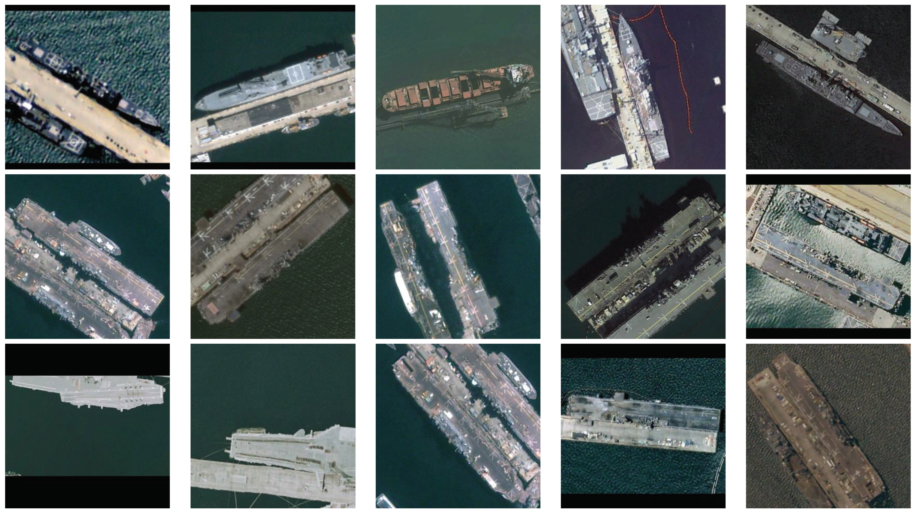
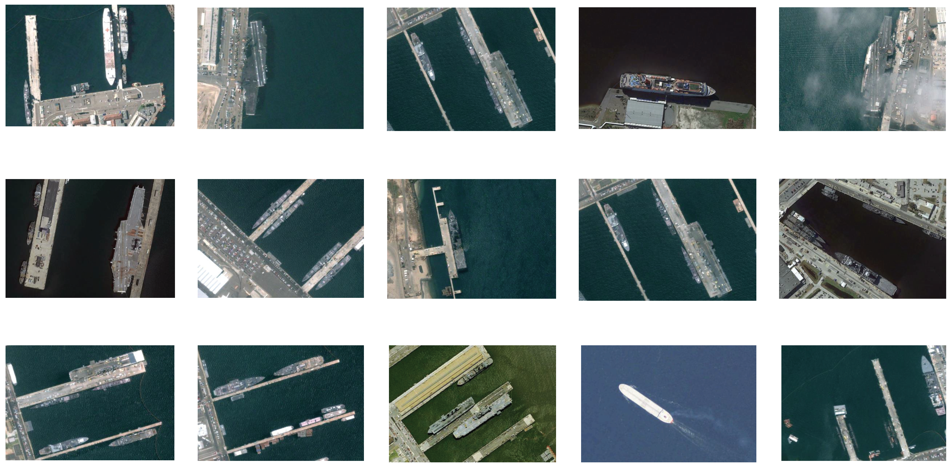
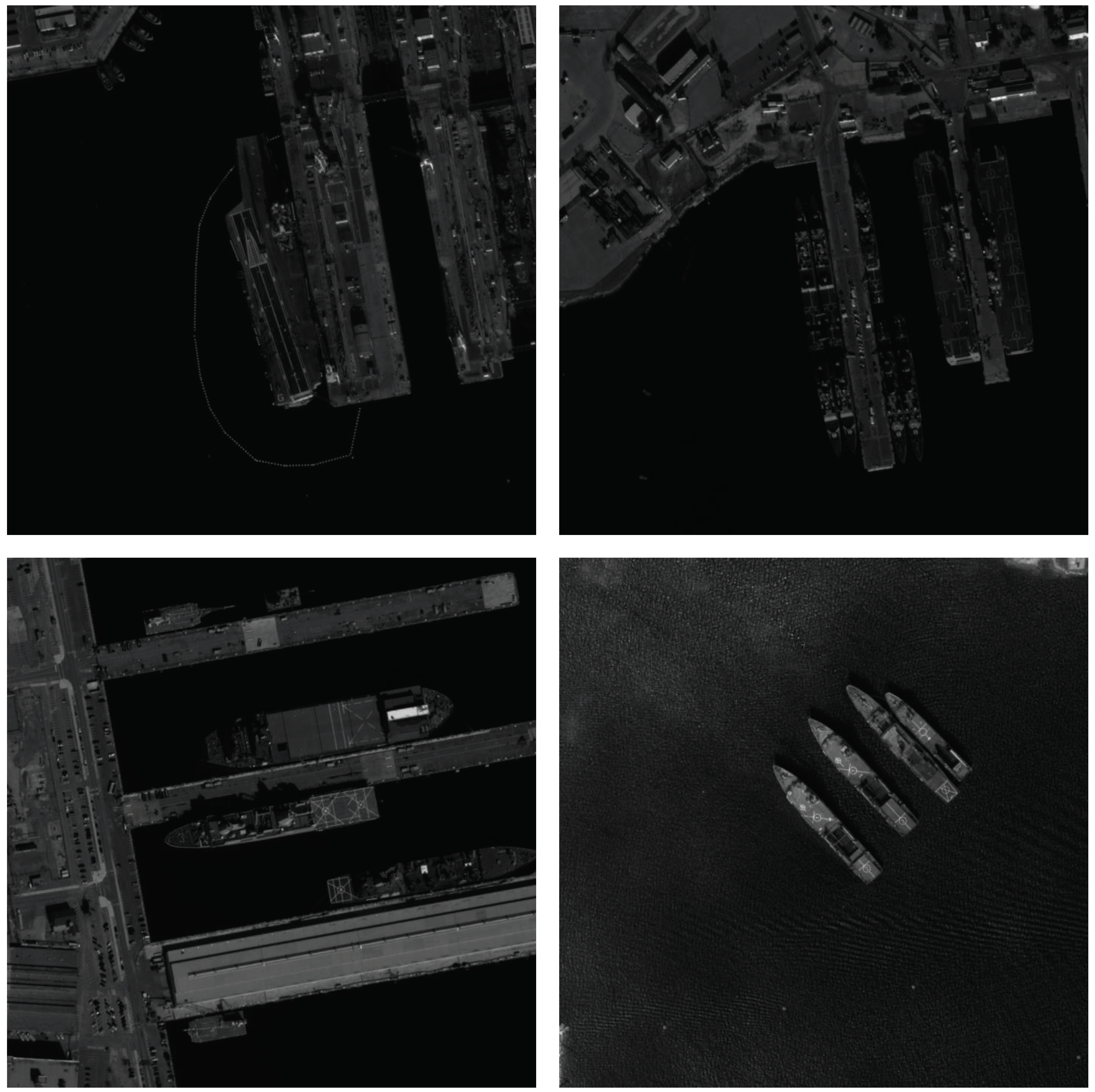
Intraclass diversity and interclass similarity between different ships. As shown in Figure 1, ships of the same type often show great differences in different environments, and some ships of different categories may be relatively similar.

(3)

Large scale differences between ships. There are large differences in size between ships.

Existing ship detection algorithms [10,11,21,22,23,24] may work unsatisfactorily when lacking training data. Due to great application significance of few-shot ship detection, researchers have conducted extensive research on the problem of less data for training. Many few-shot algorithms are proposed to solve the problem of insufficient training data. Inspired by the few-shot object detection work [25] in computer vision domain, we propose a few-shot multi-class ship detection algorithm with an attention feature map and multi-relation detector (AFMR) for the task of ship detection in remote sensing images. The input of the model are several close-up images of the target and the images to be detected. We call the close-up images support images and the images to be detected query images. Firstly, we obtain feature maps of support images and query images through a weight shared CNN feature extractor. Then, we use the feature vector from the support images to conduct depth-wise convolution on the feature map of the query map to obtain the final feature map. After that, the attention feature map is sent to the module of candidate box generation and the method of generation of the candidate box is the same as YOLO. At last, we compare the feature of the candidate boxes and the feature of support images by multi-relation detector to ascertain the position and the category information of the objects. In short, the contributions of this paper could be summarized as follows.

(1)

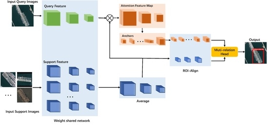
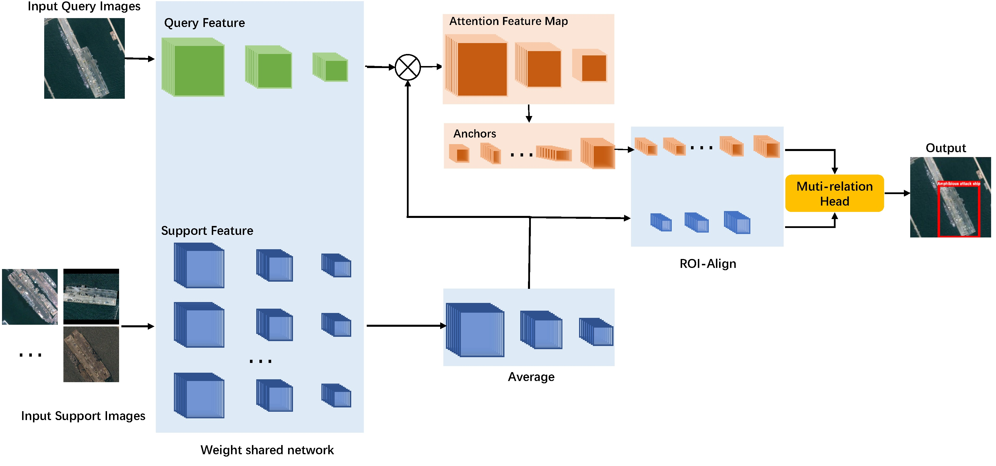
We introduce the few-shot object detection framework of [25] to the remote sensing domain and propose a few-shot multi-class ship detection algorithm with attention feature map and multi-relation detector. It solves the problem of insufficient training sample in real remote sensing ship detection application. Different from most ship detection works, treating all ships as one category, our model can achieve fine-grained classification of the detected ships.

(2)

We consider the advantage of one-stage object detection, we remove the regional proposal network in [25], and we use YOLO as the weight-shared framework to speed up ship detection.

(3)

We perform extensive experiments to evaluate our method. Experimental results show that our model achieves state-of-the-art performance, and every part of the algorithm is effective.

2. Related Works

2.1. Object Detection in Computer Vision

Object detection has always been a research hotspot in the field of computer vision, and it is also one of the most difficult tasks in computer vision. As the development of deep learning, convolutional neural networks (CNNs) have been one of the most popular models to address the tasks of computer vision, such as semantic segmentation [26,27], image classification [28,29], object detection [5,30], and so on. The anchor-based object detection algorithms based on deep learning are mainly divided into one-stage object detection algorithms and two-stage object detection algorithms. As the name suggests, two-stage object detection algorithms need two steps to complete the detection task. The main idea of two-stage method is to generate a series of candidate boxes through the selective search or the CNN network, and then classify and regress these candidate boxes. The advantage of the two-stage method is high accuracy. One-stage object detection algorithms only need one step to complete the detection task. The main idea of one-stage method is uniformly sampling evenly in different positions of the image. Different scales and length–width ratio are used in sampling, and then CNN is used to extract the features. As the whole process only needs one step, the biggest advantage of the one-stage method is high processing speed. However, an important disadvantage of uniform intensive sampling is that the training is more difficult. The reason for this phenomenon is positive samples and negative samples are extremely unbalanced, and result in a slightly low model accuracy.

The most famous two-stage object detection algorithm is the R-CNN series. R-CNN [3], which is a very early object detection algorithm using CNNs, first selects some regional proposals by the way of selective search, and then transmits these regional proposals into the CNN model to determine their categories. Fast R-CNN [4] is improved on the basis of R-CNN [3], enhancing the detection performance. It extracts the characteristics on the entire original input images, rather than extracting on each regional proposal. Following Fast R-CNN, Faster R-CNN [5] is proposed and provides great progress. In Faster R-CNN, regional proposal network (RPN) is proposed to generate proposals, which make the object detection task completely reliant on the neural network end-to-end. At the same time, the introduction of RPN greatly reduces the amount of calculation and accelerates the calculation speed of the model. Mask R-CNN [6] is an extension of Faster RCNN which introduce ROI-Align to increase precision of features of each proposal, and it adds a branch for segmentation tasks. For single-stage object detection algorithm, popular algorithms include YOLO [1] and SSD [2]. The YOLO v4 [31] algorithm predicts the offset between bounding box and box prior, which is easier to train. For the purpose of tackling problem of different scales of the objects, YOLO v4 applies multi-scale prediction. Compared to YOLO, SSD directly uses CNNs to detect target, rather than detecting after full-connection layer.

The above algorithms represent the current status of the object detection field, indicating that the current object detection algorithm has reached a very mature stage.

2.2. Ship Detection in Remote Sensing Images

Existing ship detection algorithms are generally improved versions of the classical object detection algorithms. Ref. [10] considered the characteristics of remote sensing images and improved the detection performance of YOLO v2 [32] for remote sensing objects. Tang et al. [21] used wavelet coefficients extracted from JPEG2000 compressed domain combined with deep neural network (DNN) and extreme learning machine (ELM) to solve the ship detection problem in remote sensing images. Zou et al. [22] proposed SVD Net, which is designed based on CNN and the singular value decompensation (SVD) algorithm. Li et al. [11] added hierarchical selective filtering layers to Faster R-CNN [5] to solve the problems caused by different ship scales. Yang et al. [23] proposed a ship detection algorithm which distinguished ship features through saliency segmentation and the local binary pattern (LBP) descriptor. In [24], a new rotation-invariant layer is added to R-CNN to tackle the problem of different orientations of objects. Liu et al. [33] improved the ship detection performance by redesigning the sizes of anchor boxes, predicting the localization uncertainties of bounding boxes, introducing the soft non-maximum suppression, and reconstructing a mixed loss function. Zhao et al. [34] proposed the attention receptive pyramid network (ARPN) to solve the problem of multi-scale ships detection.

However, the existing ship detection works may not be able to solve the problem of few-shot detection of multi-type ships in remote sensing images.

2.3. Few-Shot Object Detection

The existing object detection task is based on a large number of samples with labels. This requirement limits the application and promotion in some scenes. To train a model that has a certain generalization ability with few samples is the major task of small sample learning. Therefore, the research of few-shot learning has a great significance. There are many excellent works in few-shot object detection. Researchers mainly solve the problem of few-shot learning by fine-tuning, metric learning, and meta learning. Leonid Karlinsky [35] et al. proposed a method to equip an object detector with a distance metric learning (DML) classifier head that can admit new categories. Kang et al. [36] proposed a model including meta feature learner and a re-weighting module within a one-stage detection architecture. Wang et al. [37] divided the training into two parts. The first is base training, which trains the whole model on base classes. The second is few-shot fine-tuning, which fine-tunes the last layer and freezes other parameters with smaller learning rates. Fine-tuning is widely used in few-shot detection, which fixes the feature extraction part and only adjusts the classification and regression parts after the model is trained on base classes. The feature extraction part extracts some general features in base classes. Though some categories may not appear in the base categories, some features analoging with those general features may have been learned by the network. The network re-weights and arranges these features in the subsequent stage then combines them into the features of a new class of objects. Chen et al. [38] propose LSTD to solve the difficulty of sample scarcity. In LSTD, SSD is used to design bounding box regression, and there is a default candidate box for each layer. Each layer uses smooth L1 to train the box regression. Faster RCNN is used to design target classification. For the default box, the classification score is used to select the target proposal of the RPN. Then, the ROI is applied to the middle layer of the convolutional network to generate fixed-size convolutional features for each proposal. Finally, two convolutional layers are used to replace the original fully connected layer of the Faster RCNN. Dong et al. [39] proposed a method of using a small data set with labels and a large data set without labels to train object detection networks. This method solves the problem that few-shot object detection is easy to fall into a local optimal solution. Fan et al. [25] raised a new few-shot object detection model based on Faster R-CNN. The attention mechanism is added to RPN in the model, and the multi-relation detector is used as detection head. Fan et al. [40] proposed Retentive R-CNN consisted by Bias-Balanced RPN and re-detector to tackle the problem of forgetting base categories. Zhu et al. [41] investigated utilizing the semantic relation of the novel categories and base categories together with the visual information and proposed SRR-FSD to solve the problem of variation of shots of novel objects.

Nevertheless, compared with the object detection algorithm with sufficient samples, the few-shot detection algorithm still has much room for improvement.

2.4. Few-Shot Learning in Remote Sensing Images

Due to the important application value of remote sensing images, researchers are committed to studying few-shot learning algorithms for remote sensing images. Initially, researchers use data augment (DA) methods to solve the problem of data scarcity. Li et al. used methods of cropping and flipping to increase the number of samples. DA. C. M. Ward et al. [42] introduced synthetic images made from 3D ship models. The synthetic images were used as auxiliary information to enhance the features of the samples to improve the performance of the model. When the method of data enhancement developed to reach the bottleneck, other methods were used to tackle the difficulties, such as improving models, transfer learning [43], meta-learning, and so on. Ai et al. [44] proposed a SAR image target detection method based on a multi-level depth learning network which fuses the high-level target depth feature extracted by the traditional Haar template with the high-level target depth feature extracted by the conventional depth convolutional neural network, not only effectively improves the characterization of the SAR image targets, but also improves SAR image target detection accuracy with small dataset. Aiming at the problem of classifier degradation caused by missing samples, Shi et al. [17] proposed a few-shot ship classification method based on prototype representation and achieved high classification accuracy. Li et al. [18] proposed a meta-learning model for remote sensing image object detection. The model uses a meta-feature extractor to extract the meta-features of the input image and uses the re-weighted vectors obtained from the support images to correct the meta-features. The model achieves satisfying results on two benchmark datasets. Huang et al. [19] used transfer learning method to handle the problem of scarce labeled SAR images, which transferred the knowledge from pretraining a network with sufficient unlabeled SAR scene images to scarce labeled SAR images. Zhang et al. [20] introduced semantic information in the zero-shot learning task, which achieved a better ship detection effect. M Rostami et al. [45] proposed a new algorithm to solve the problem of ship classification with limited data. Zhang et al. [46] proposed a few-shot object detection algorithm based on the YOLO algorithm which achieved a better result. Hao et al. [47] proposed a few-shot ship detection algorithm which achieved high detection accuracy and real-time performance.

In short, comparing to the methods described above, our approach is committed to solving the task of few-shot multi-class ship detection in the remote sensing image, and does not require pretraining and other domain data.

3. Methods

The structure of our framework is shown in Figure 2. In the rest of this section, we will introduce the settings in the task of few-shot object detection and present every part of our model in detail.

3.1. Introduction of Settings

In our method, the input of our model is divided into two parts. The first part is called support image which contains a close-up of the target. Moreover, we call the set of support images as support set. The second part of input is called query image which contains the target in the support image. Compared to support image, the size of query image is larger than support image. Similarly, we call the set of query images a query set. Our goal is to find the target in the query image that belonging to support images and to give the information of location and category. If we have N categories in our test set, and each category has K images, we call the task as N-way K-shot detection [35].

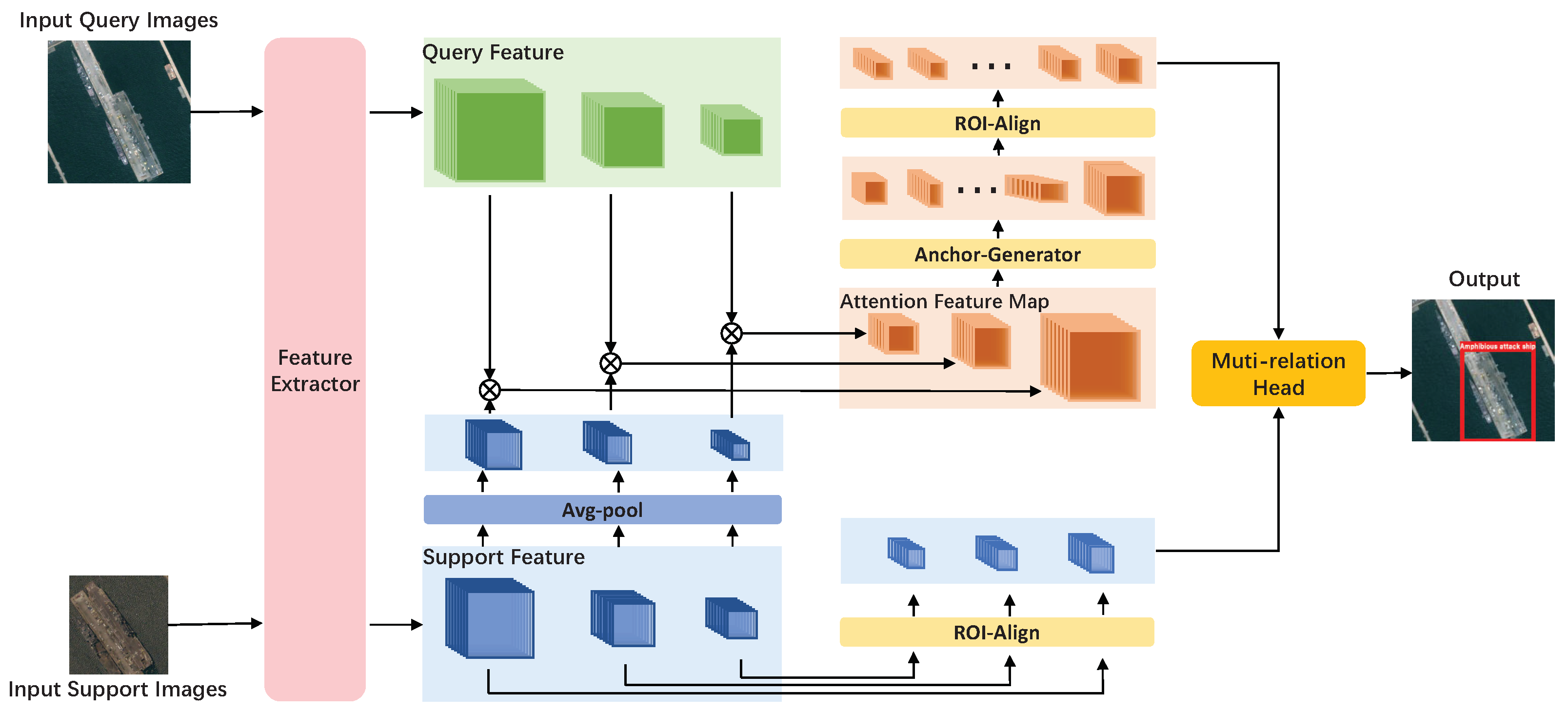
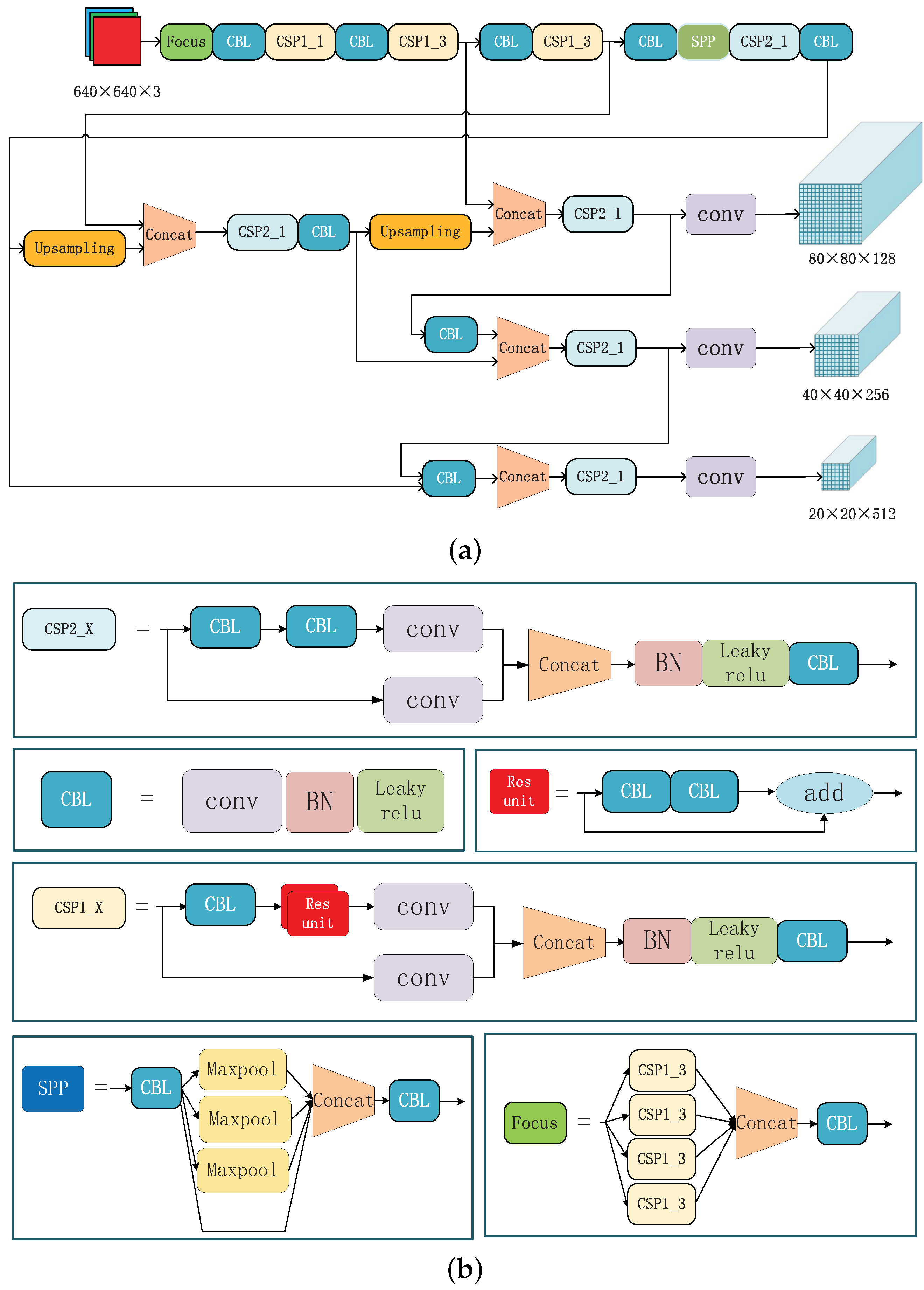
3.2. Feature Extractor

In an N-way K-shot problem, the input of feature extractor will have $K+1$ branches (one branch for one image), one of them for one query image and the others for K support images (K support images for each category). It is necessary to notice that, in order to expression, the branch of support image in Figure 2 only has one channel. Our feature extractor has two parts. The first is weight shared network [48], while the second is feature map fusion. Considering the powerful feature extraction capability, weight shared network uses improved Dark-Net which is the backbone of YOLO [1], as shown in Figure 3. Considering the scale difference among objects, the weight shared network will extract three feature maps of different scales in each branch. After the weight shared network, we will have $K\times 3$ feature maps of support images and 3 feature maps of the query image. For $K\times 3$ feature maps of support images of each category, we calculate the average on the feature maps of the same scale by channel in feature map fusion part. So, after the feature extractor, we find 3 average representations of feature maps of K support images and 3 feature maps of the query image.

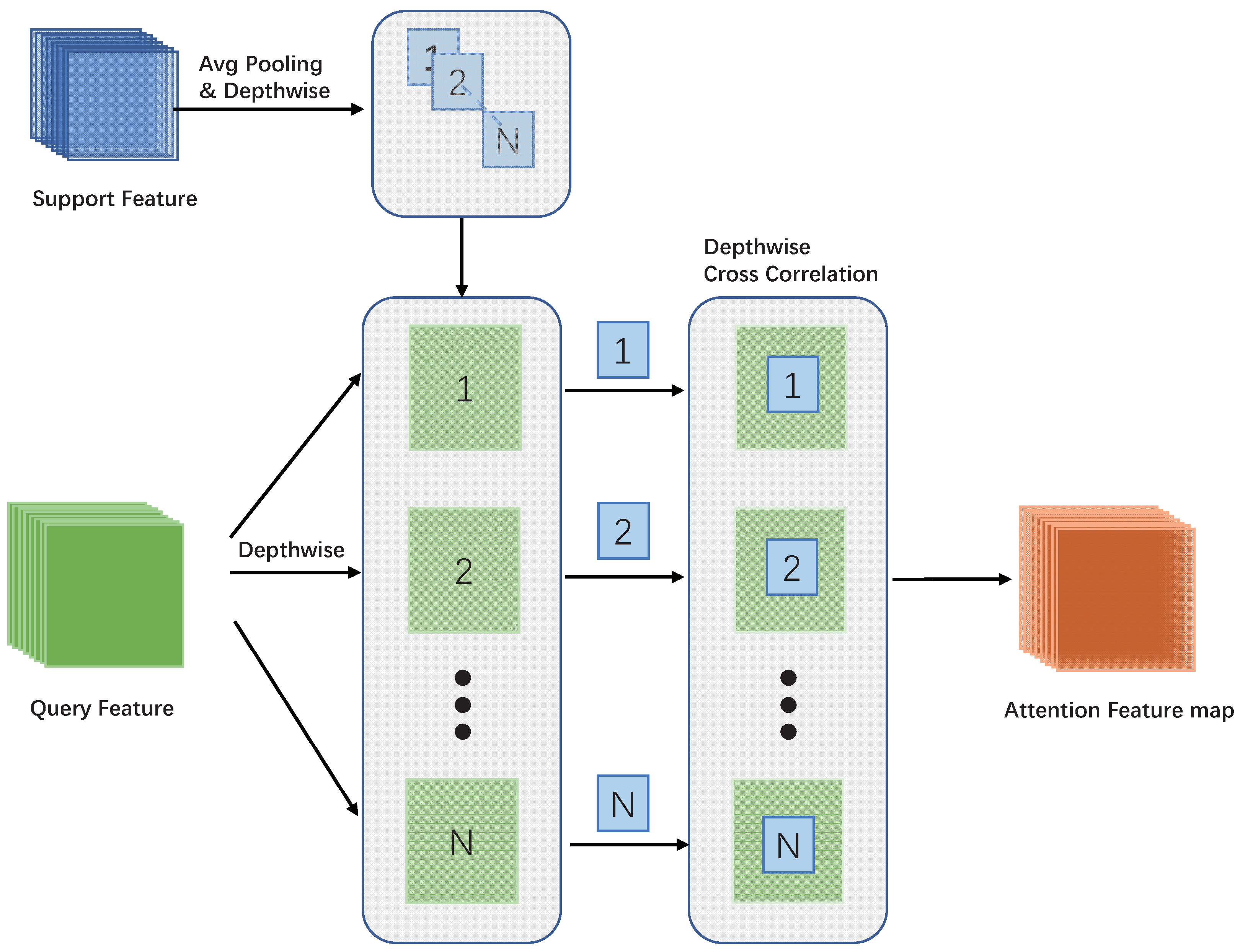
3.3. Attention Feature Map

For each input class, we obtain three feature maps of different scales of the target. In addition, we also gain three different feature maps of the query image. We define the average representation of feature maps of support images as $S_k\in t^{b_k\times b_k\times c_k}$ and the feature maps of query images as $Y_k\in t^{h_k\times h_k\times c_k}$, where $k=1,2,3$ represents the scale of feature map. Then, we perform average pooling on $S_k$, and find the average representation of feature maps of support images defined as $S_{ka}\in t^{a_k\times a_k\times c_k}$. Moreover, we can compute the similarity of support images and the query images as

$$G_{h,w,c,k}=\sum _{i,j}{S}_{i,j,c,k}·Y_{h+i-1,w+j-1,c,k},i,j\in \left[1,\cdots ,a_k\right]$$

where $G_{h,w,c,k}$ is attention feature map. We regard the support feature map $S_{ka}$ as a convolution kernel and use it to slide on the feature map of the query image $Y_K$ in a depth-wise cross correlation way. After that, $G_{h,w,c,k}$ will be sent to the module of candidate box generation. In the module of candidate box generation, we adopt the same way with YOLO [1]. The structure of the attention feature map is shown in Figure 4.

3.4. Multi-Relation Head

After finding candidate boxes, we perform ROI align on the support features $S_{ka}$ and the feature map corresponding to the candidate box we have. As we have support feature maps of three scales, we need to perform ROI align to fix the shape depending on the scale of support feature maps. After that, we find one of the input $S_{rk}$. Corresponding to support feature maps, the candidate boxes will be obtained after ROI align on the corresponding scale according to its own scale, and then we have $Y_{rk}$, where $k=1,2,3$. Finally, we input $S_{rk}$ and $Y_{rk}$ into multi-relation detector. The so-called multi-relation head is to compare the similarity of $S_{rk}$ and $Y_{rk}$ from three aspects. They are global-relation head, local-relation head, and patch-relation head. The global-relation head uses a global representation to match images; the local-relation head captures pixel-to-pixel matching relations, and the patch-relation head models one-to-many pixel relations. Their specific operations are as follows.

• Global-relation head. Firstly, we concatenate $S_{rk}$ and $Y_{rk}$ to find the concatenated feature $F_c$ whose size is $m\times m\times 2c$. Then we perform global average pooling on $F_c$ and $F_c$ becomes a $1\times 1\times 2C$ vector. Then we input $F_c$ to a network which contains MLP with two fully connected layers with ReLU and a final fully connected layer and generate a matching score.
• Local relation head. Firstly, we use a weight shared convolution kernel to perform channel-wise convolutional operation on $S_{rk}$ and $Y_{rk}$. Then, we use the two feature maps to perform depth-wise convolutional. Then, we find a matching score after a fully connected layer.
• Patch relation head. We concatenate $S_{rk}$ and $Y_{rk}$ firstly, and find the concatenated feature $F_c$ whose size is $m\times m\times 2c$. Then we put $F_c$ into a module and the structure of the module is shown as

  Table 1. Architecture of the module in patch-relation head with the input size $7\times 7$. Avg Pool means average pooling. Conv means convolution layer. All the convolution layers followed by ReLU. s1 means the stride is 1 and p0 means the padding is 0.

  Type	Filter Shape	Stride/Padding
  Avg Pool	$3\times 3\times 4096$	$s1/p0$
  Conv	$1\times 1\times 512$	$s1/p0$
  Conv	$3\times 3\times 512$	$s1/p0$
  Conv	$1\times 1\times 2048$	$s1/p0$
  Avg Pool	$3\times 3\times 2048$	$s1/p0$

  . The size of the output of the module is $1\times 1\times 2C$. Finally, we put the output into a fully connected layer to generate matching score and put the output into another fully connected layer to generate bounding box information.

4. Experiments and Results

In order to verify the effectiveness of our method, in this section we introduce the remote sensing dataset we used in the experiments and evaluate the performance of our model. We also compare our model with other detectors. It should be noticed that our data and code will be released to the public via the first author’s webpage (https://haopzhang.github.io/, accessed on 26 April 2022).

4.1. Datasets

In order to test our model for the task of few-shot multi-class ship detection, a remote sensing image dataset containing numerous ship categories is needed. Several public remote sensing datasets commonly used by researchers are DOTA [49], NWPU VHR-10 [50], LEVIR [51], and HRSC2016 [52]. We compare these four datasets in

Table 2. Comparison of four commonly used remote sensing datasets and comparison of the ship data they containing.

Dataset	Categories Numbers	Categories	Categories Number of Ships	Categories of Ships	Ship Numbers
NWPU VHR-10	10	Airplane, storage tanks, ship, baseball fields, ground runways, etc.	1	Ship	302
DOTA	15	Airplane, bridge, swimming pool, ship, roundabout, etc.	1	Ship	6300
LEVIR	3	Airplane, ship, oilpot	1	Ship	3025
HRSC2016	19	Medical boat, Ticonderoga, Nimitz, Perry, Austin, etc.	19	Medical boat, Ticonderoga, Nimitz, Perry, Austin, etc.	2010

. As we can see, DOTA [49], NWPU VHR-10 [50], and LEVIR [51] contain various categories of targets, but these three datasets all regard ships as one category without specific labels within ship category. HRSC2016, the short of High Resolution Ship Collection 2016, is suitable for the task of ship detection. Images in HRSC2016 are cropped from Google Earth and they are all from six famous harbours. In addition to the bounding box annotation, it also contains three level labels: ship, ship category, and ship types. Although HRSC2016 have sufficient categories of ship and numerous samples, the first 4 types (Ship, Aircraft Carrier, Warcraft, and Merchant Ship) out of 19 are confused with the following 15 types, e.g., Kitty Hawk class aircraft carrier belongs to aircraft carrier, and Arleigh Burke class destroyer belongs to warcraft. Thus, we conduct our experiments on HRSC2016 with the rest 15 ship types. Sample ship images in each class in HRSC2016 are shown in Figure 5.

To verify the generalization of our model, we also collect a self-constructed dataset called REMEX-FSSD, where REMEX is the name of our lab (https://remex-lab.github.io/index.html (accessed on 16 April 2022)) and FSSD means few-shot ship detection. REMEX-FSSD contains four categories of ship and 14,252 images. All images are collected from the panchromatic band of WorldView satellite. Sample distribution of REMEX-FSSD is shown as

Table 3. Sample distribution of REMEX-FSSD dataset.

Category	Aircraft Carrier	Amphibious Attack Ship	Destroyer	Others	Total
Number	1357	3675	26,961	24,546	56,539

. We show each class of ships in REMEX-FSSD in Figure 6.

4.2. Experimental Setup

In order to test the performance of our model in ship detection with few-shot setting, we split the dataset we used into two parts: one contains base classes and the other contains novel classes. For the 15 selected classes in HRSC2016 dataset, we set five classes as novel classes (Kitty Hawk class aircraft carrier, Arleigh Burke class destroyers, Sanantonio class amphibious transport dock, Abukuma-class destroyer escort, and Medical ship) and the others are base classes. For REMEX-FSSD, we regard aircraft carrier, amphibious ship, and others as base classes and the destroyer as novel class. During the training phase, we train the model on the base classes. After training on the base classes, we fix the weights of the feature extractor and only fine-tune the high level layers with the novel classes. Our model is trained end to end with Adam [53] optimizer. The learning rate is initialled to $1\times {10}^{-3}$ and is halved in the last 50 epochs.

All experiments mentioned in this paper were conducted in Python with PyTorch and ran on a computer with two CPUs of Intel (R) Xeon (R) CPU E5-2630 v4 @2.20 GHz and four GPUs of NVIDIA GeForce GTX 1080Ti.

4.3. Evaluation Indicators

For object detection tasks, the average precision mAP 50 (mean Average Precision) is generally adopted as the performance verification metric. We will introduce the calculation process of mAP in detail in this section.

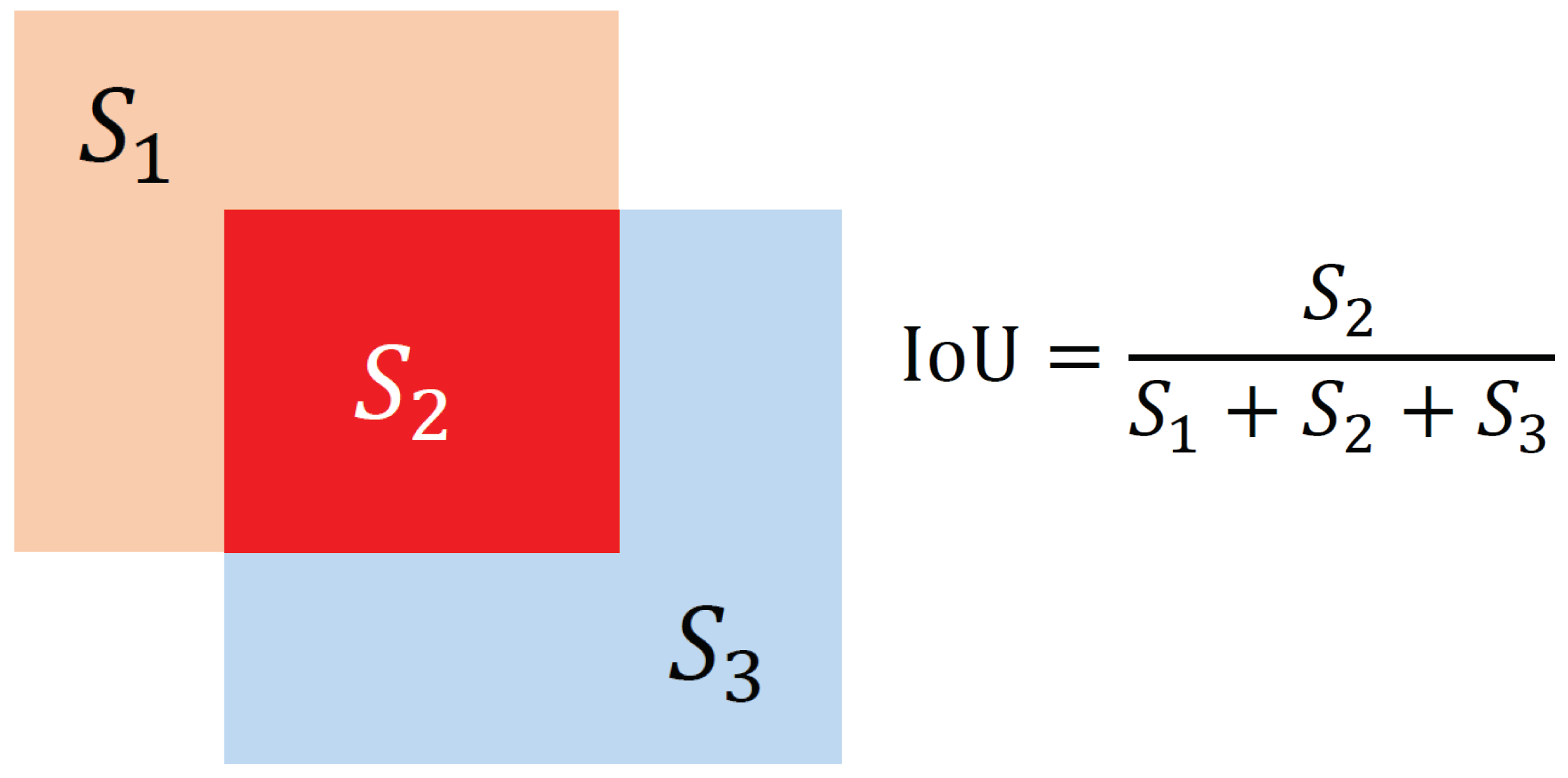
• IoU (Intersection over Union): IOU refers to the ratio of the area of the overlapping part of the prediction box and the ground-truth box to the area occupied by their union. The calculation process of IoU is shown in Figure 7, where $S_1$ represents the area of the orange area, $S_2$ represents the area of the red area, and $S_3$ represents the area of the blue area.
• Precision and Recall: When the confidence of the prediction box is greater than the confidence threshold, the prediction box is called Positive. Otherwise, it is called Negative. When the IoU of the prediction box and the ground truth box is greater than the threshold, the prediction box is called True, otherwise it is called False. Based on this, the discrimination methods of TP, FP, TN, and FN are shown in

  Table 4. The discrimination methods of TP, FP, TN, and FN.

  	Positive	Negative
  True	TP	TN
  False	FP	FN

  .
  Therefore, the calculation method of the precision rate and the recall rate is shown as:

  $$Precision=\frac{TP}{TP+FP}$$

  $$Recall=\frac{TP}{TP+FN}$$
• Drawing PR curve and calculating mAP. After obtaining the PR curve, the area enclosed by the PR curve and the coordinate axis is the AP value of each category. After obtaining the AP value of each category, the AP of all categories is added and averaged, where mAP 50 means that the IoU threshold is taken as 0.5 during the calculation.

4.4. Results

We compared our method with four object detection methods including Faster-RCNN [5], YOLO [1], FSOD [25], and TFA [37]. The first two are classic object detection algorithms, while the other two are state-of-the-art few-shot object detection algorithms.

The performance of each method with 5-way 5-shot is shown in

Table 5. The performance of different methods on HRSC2016. Class 1–Class 5 represent Kitty Hawk class aircraft carrier, Arleigh Burke class destroyers, Sanantonio class amphibious transport dock, Abukuma-class destroyer escort, and Medical ship, respectively. AF means attention feature map mentioned in Section 3.3, FC means Fully-Connected-layer-based classifier and COS means cosine-similarity-based classifier.

Method	mAP 50	Class 1	Class 2	Class 3	Class 4	Class 5
Faster-RCNN [5]	2.1	2.3	1.7	3.4	0.3	2.8
YOLO [1]	1.94	2.1	1.4	3.0	0.4	2.8
Faster-RCNN + AF	3.52	4.1	2.8	5.1	1.6	3.3
YOLO + AF	3.78	3.9	3.4	5.5	1.2	4.9
FSOD [25]	15.68	16.9	14.7	19.2	10.3	17.3
TFA/FC [37]	23.59	26.63	23.37	28.13	18.68	21.14
TFA/COS [37]	26.82	28.81	26.7	32.49	21.37	24.73
Ours	27.08	31.5	25.6	34.9	17.3	26.1

. It is well known that the task of object detection include two subtasks: location and classification. Considering the datasets we used have different kinds of ships, the classification subtask in our experiment can be regarded as fine-grained ship classification. Due to huge intraclass diversity and interclass similarity, such a ship detection task is more difficult than general object detection.

As shown in the first two rows of Table 5, the performances of two classic object detection methods Faster-RCNN and YOLO degrade seriously in a few-shot scenario due to insufficient training data. The lower indicator proves that the classical object detection algorithm cannot be directly used in the task of few-shot object detection. In the third and the forth rows of Table 5, we add an attention feature map to Faster-RCNN and YOLO, and their performance improves slightly. The fifth to the seventh rows are state-of-the-art few-shot object detection algorithms. They both adopt Faster-RCNN as basic detection model but use different ideas for improvement. TFA applies the fine-tuning method, while FSOD, similar to metric learning, adopt the structure of Siamese network. As shown in Table 5, TFA is better than FSOD.

Compared with other few-shot algorithms, our method performs the best. Among the novel classes we set (five categories in total), we achieve the highest detection performance for three categories and find the best mAP 50 of $27.08\%$, an improvement of $0.26\%$ over $26.82\%$, the second best TFA/COS.

In order to verify the generalization of our model, we also conduct experiments on REMEX-FSSD. The performance of our method is shown in

Table 6. The performance of different methods on REMEX-FSSD.

Method	mAP 50
Faster-RCNN [5]	10.7
YOLO [1]	8.24
FSOD [25]	26.73
TFA/fc [37]	34.33
TFA/cos [37]	35.74
Ours	38.12

. Generally, the performance of each method on REMEX-FSSD is better than the performance shown in Table 5. The reason for the performance change is that the category number of REMEX-FSSD is smaller than HRSC2016 (15 versus 4). However, the performance ranking among the algorithms on REMEX-FSSD dataset remains the same as that on HRSC2016. Comparing with the second highest indicator by TFA/COS, our method achieves $38.12\%$, an improvement of $2.38\%$ over $26.82\%$.

In order to verify the stability of our model, we repeatedly tested our model five times.

Table 7. Stability verification experiment.

Dataset	HRSC2016	REMEX-FSSD
1	27.08	38.12
2	27.06	38.11
3	27.10	38.10
4	27.04	38.14
5	27.10	38.12
Average	27.076	38.118
Standard deviation	0.023	0.013

shows that the five experimental index values and their average and standard deviation. It can be seen that our model performs stably with each of the two datasets.

In order to verify the calculation speed of the model, we organized experiments to compare the running speed of our algorithm with others.

Table 8. Speed comparison of different methods on HRSC2016 and REMEX-FSSD datasets. FPS means frame per second.

Method	HRSC2016 (FPS)	REMEX-FSSD (FPS)
Faster-RCNN [5]	11.9	13.2
YOLO [1]	30.6	36.1
FSOD [25]	10.8	11.9
TFA/cos [37]	12.1	13.3
Ours	27.8	33.2

shows the comparative results of these experiments.

4.5. Ablation Study

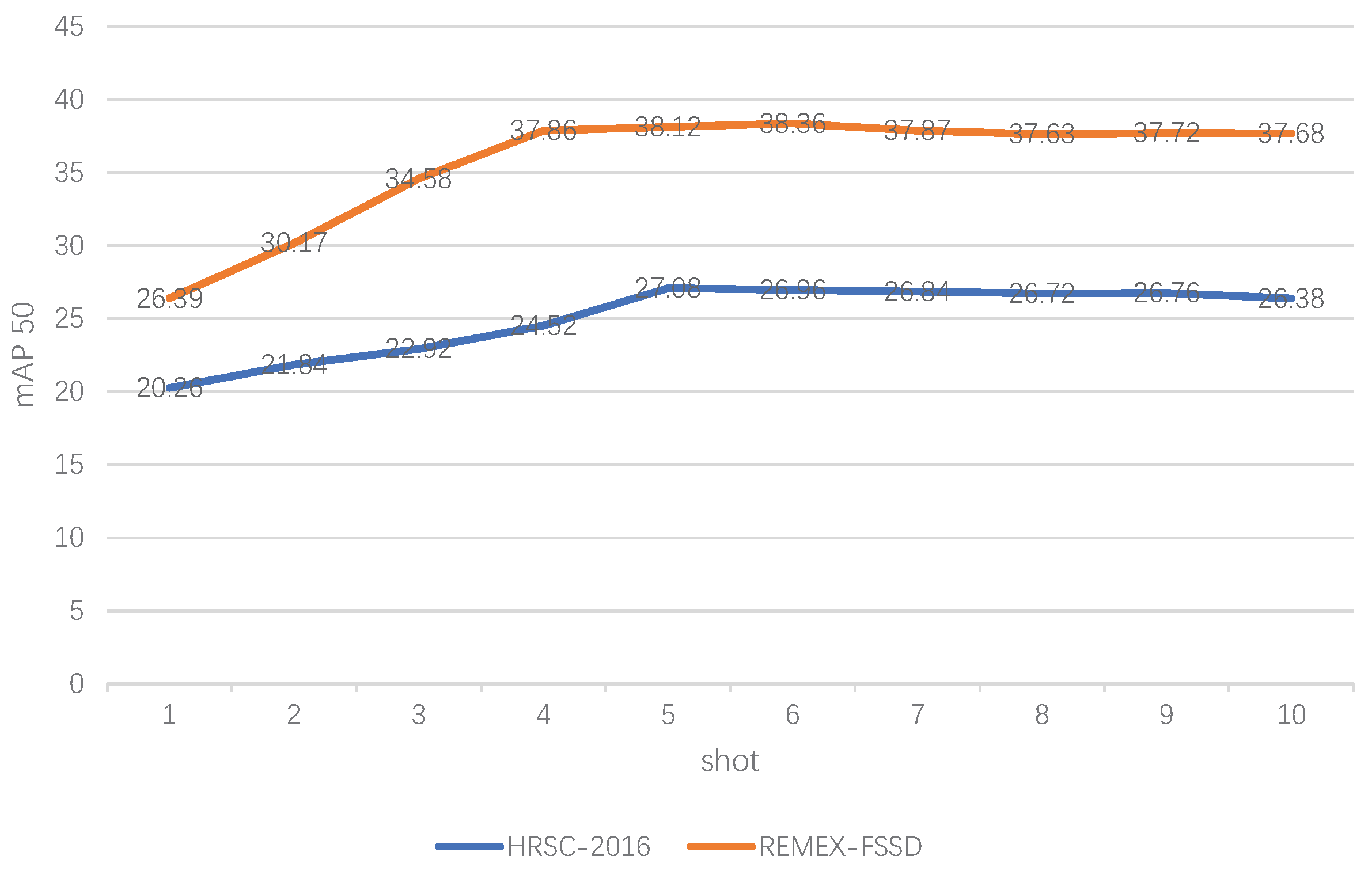
4.5.1. Number of Training Samples

We performed experiments to find that how many shots on the unseen classes are needed for our algorithm. We conducted comparative experiments from 1-shot to 10-shot on two datasets, HRSC2016 and REMEX-FSSD, respectively. As shown in Figure 8, 5-shot is the best setting for the HRSC2016 dataset and 6-shot is the best setting for the REMEX-FSSD dataset. Figure 9 and Figure 10 show the selected detection results on HRSC2016 and REMEX-FSSD, respectively.

4.5.2. Role of Different Modules

We conducted experiments for ablation study to verify the role of each module in our method. As

Table 9. Ablation study of different modules in the 5-way 5-shot training strategy on HRSC2016. AF means attention feature map and MR means multi-relation head.

YOLO	AF	MR	mAP50
√	-	-	1.94
√	√	-	3.78
√	-	√	11.36
√	√	√	27.08

shows, the attention feature map and the multi-relation head both benefit the performance of the algorithm. The module of multi-relation head brings a $9.42\%$ improvement (from $1.94\%$ to $11.36\%$). In particular, the best detection results are achieved when both an attention feature map and multi-relation head are added to the model.

4.5.3. Combinations of Different Relation Heads

We also conducted experiments to explore the influence of each relation head. As shown in

Table 10. Ablation study of relation heads. Experimental results under different detection head combinations are achieved in the 5-way 5-shot training strategy on HRSC2016.

Global R	Local R	Patch R	mAP50
-	-	-	3.78
√	-	-	21.63
-	√	-	23.26
-	-	√	20.17
√	√	-	26.73
√	-	√	22.37
-	√	√	25.82
√	√	√	27.08

, each relation head of the multi-relation head is useful. When there is only one detection head, the boosting effect of local relation head is the best, and the effect of patch relation head is the smallest. When randomly combining two types of relation heads, we achieve better results than the performance with one of the two relation heads. The algorithm achieves the best results when the entire multi-relation head is used among all different combinations of all the three relation heads.

4.6. Discussion

According to our ablation study, a multi-relation head greatly improves the algorithm, and the three different relation heads promote each other and achieve the best detection results. Experiments on HRSC2016 and REMEX-FSSD datasets prove the effectiveness and advancement of our method. Compared with other state-of-the-art few-shot object detection algorithms, our method performs better under the same experiment settings. Considering that multi-relation head, especially local-relation head, brings a huge improvement in detection performance, we think that the detection head plays a decisive role in few-shot ship detection.

5. Conclusions

In this paper, we have proposed a few-shot multi-class ship detection algorithm with an attention feature map and multi-relation detector (AFMR) to solve the problem of ship detection in remote sensing images. We added a feature attention map module with Siamese network architecture and multi-relation head to the base architecture. In the feature attention map module, we constructed an attention feature map by using the average pooled support features to enhance the features of objects in query images. Through such operation, the activation value of the area that looks like the support image on the query image will be very high, so that it is easy to find highly suspected areas on the query image. In the module of multi-relation head, the input are support feature and the feature of candidate area aligned by the ROI-align. In future work, we plan to improve existing detection heads and study metric-based detection heads to achieve better performance for few-shot multi-class ship detection in remote sensing images.

References

1. Redmon, J.; Divvala, S.; Girshick, R.; Farhadi, A. You Only Look Once: Unified, Real-Time Object Detection. In Proceedings of the 2016 IEEE Conference on Computer Vision and Pattern Recognition (CVPR), Las Vegas, NV, USA, 27–30 June 2016; pp. 779–788. [Google Scholar] [CrossRef] [Green Version]
2. Liu, W.; Anguelov, D.; Erhan, D.; Szegedy, C.; Reed, S.; Fu, C.Y.; Berg, A.C. SSD: Single Shot MultiBox Detector. In European Conference on Computer Vision; Lecture Notes in Computer Science; Springer: Cham, Switzerland, 2016; pp. 21–37. [Google Scholar] [CrossRef] [Green Version]
3. Girshick, R.; Donahue, J.; Darrell, T.; Malik, J. Rich Feature Hierarchies for Accurate Object Detection and Semantic Segmentation. In Proceedings of the 2014 IEEE Conference on Computer Vision and Pattern Recognition, Columbus, OH, USA, 23–28 June 2014; pp. 580–587. [Google Scholar] [CrossRef] [Green Version]
4. Girshick, R. Fast R-CNN. In Proceedings of the 2015 IEEE International Conference on Computer Vision (ICCV), Santiago, Chile, 7–13 December 2015; pp. 1440–1448. [Google Scholar] [CrossRef]
5. Ren, S.; He, K.; Girshick, R.; Sun, J. Faster R-CNN: Towards Real-Time Object Detection with Region Proposal Networks. IEEE Trans. Pattern Anal. Mach. Intell. 2017, 39, 1137–1149. [Google Scholar] [CrossRef] [PubMed] [Green Version]
6. He, K.; Gkioxari, G.; Dollár, P.; Girshick, R. Mask R-CNN. In Proceedings of the 2017 IEEE International Conference on Computer Vision (ICCV), Venice, Italy, 22–29 October 2017; pp. 2980–2988. [Google Scholar] [CrossRef]
7. Everingham, M.; Van Gool, L.; Williams, C.K.; Winn, J.; Zisserman, A. The pascal visual object classes (voc) challenge. Int. J. Comput. Vis. 2010, 88, 303–338. [Google Scholar] [CrossRef] [Green Version]
8. Lin, T.Y.; Maire, M.; Belongie, S.; Hays, J.; Perona, P.; Ramanan, D.; Dollár, P.; Zitnick, C.L. Microsoft COCO: Common Objects in Context. In European Conference on Computer Vision; Fleet, D., Pajdla, T., Schiele, B., Tuytelaars, T., Eds.; Springer International Publishing: Cham, Swizterland, 2014; pp. 740–755. [Google Scholar] [CrossRef] [Green Version]
9. Deng, J.; Dong, W.; Socher, R.; Li, L.J.; Li, K.; Fei-Fei, L. ImageNet: A large-scale hierarchical image database. In Proceedings of the 2009 IEEE Conference on Computer Vision and Pattern Recognition, Miami, FL, USA, 20–25 June 2009; pp. 248–255. [Google Scholar] [CrossRef] [Green Version]
10. Etten, A.V. You Only Look Twice: Rapid Multi-Scale Object Detection In Satellite Imagery. arXiv 2018, arXiv:1805.09512. [Google Scholar]
11. Li, Q.; Mou, L.; Liu, Q.; Wang, Y.; Zhu, X.X. HSF-Net: Multiscale Deep Feature Embedding for Ship Detection in Optical Remote Sensing Imagery. IEEE Trans. Geosci. Remote Sens. 2018, 56, 7147–7161. [Google Scholar] [CrossRef]
12. Nie, S.; Jiang, Z.; Zhang, H.; Cai, B.; Yao, Y. Inshore Ship Detection Based on Mask R-CNN. In Proceedings of the IGARSS 2018—2018 IEEE International Geoscience and Remote Sensing Symposium, Valencia, Spain, 22–27 July 2018; pp. 693–696. [Google Scholar] [CrossRef]
13. Snell, J.; Swersky, K.; Zemel, R. Prototypical networks for few-shot learning. In Proceedings of the 31st Conference on Neural Information Processing Systems (NIPS 2017), Long Beach, CA, USA, 4–9 December 2017; Volume 30. [Google Scholar]
14. Vinyals, O.; Blundell, C.; Lillicrap, T.; Wierstra, D. Matching networks for one shot learning. In Proceedings of the 30th Conference on Neural Information Processing Systems (NIPS 2016), Barcelona, Spain, 5–10 December 2016; Volume 29. [Google Scholar]
15. Finn, C.; Abbeel, P.; Levine, S. Model-Agnostic Meta-Learning for Fast Adaptation of Deep Networks. In Proceedings of the 34th International Conference on Machine Learning, Sydney, Australia, 6–11 August 2017; Volume 70, pp. 1126–1135. [Google Scholar]
16. Nichol, A.; Achiam, J.; Schulman, J. On first-order meta-learning algorithms. arXiv 2018, arXiv:1803.02999. [Google Scholar]
17. Shi, J.; Jiang, Z.; Zhang, H. Few-Shot Ship Classification in Optical Remote Sensing Images Using Nearest Neighbor Prototype Representation. IEEE J. Sel. Top. Appl. Earth Obs. Remote Sens. 2021, 14, 3581–3590. [Google Scholar] [CrossRef]
18. Li, X.; Deng, J.; Fang, Y. Few-Shot Object Detection on Remote Sensing Images. IEEE Trans. Geosci. Remote Sens. 2022, 60, 1–14. [Google Scholar] [CrossRef]
19. Huang, Z.; Pan, Z.; Lei, B. Transfer Learning with Deep Convolutional Neural Network for SAR Target Classification with Limited Labeled Data. Remote Sens. 2017, 9, 907. [Google Scholar] [CrossRef] [Green Version]
20. Zhang, Z.; Zhoa, J.; Liang, X. Zero-shot Learning Based on Semantic Embedding for Ship Detection. In Proceedings of the 2020 3rd International Conference on Unmanned Systems (ICUS), Harbin, China, 27–28 November 2020; pp. 1152–1156. [Google Scholar]
21. Tang, J.; Deng, C.; Huang, G.B.; Zhao, B. Compressed-Domain Ship Detection on Spaceborne Optical Image Using Deep Neural Network and Extreme Learning Machine. IEEE Trans. Geosci. Remote Sens. 2015, 53, 1174–1185. [Google Scholar] [CrossRef]
22. Zou, Z.; Shi, Z. Ship Detection in Spaceborne Optical Image With SVD Networks. IEEE Trans. Geosci. Remote Sens. 2016, 54, 5832–5845. [Google Scholar] [CrossRef]
23. Yang, F.; Xu, Q.; Li, B. Ship Detection From Optical Satellite Images Based on Saliency Segmentation and Structure-LBP Feature. IEEE Geosci. Remote Sens. Lett. 2017, 14, 602–606. [Google Scholar] [CrossRef]
24. Cheng, G.; Zhou, P.; Han, J. Learning Rotation-Invariant Convolutional Neural Networks for Object Detection in VHR Optical Remote Sensing Images. IEEE Trans. Geosci. Remote Sens. 2016, 54, 7405–7415. [Google Scholar] [CrossRef]
25. Fan, Q.; Zhuo, W.; Tang, C.K.; Tai, Y.W. Few-Shot Object Detection with Attention-RPN and Multi-Relation Detector. In Proceedings of IEEE/CVF Conference on Computer Vision and Pattern Recognition (CVPR); Seattle, WA, USA, 13–19 June 2020.
26. Long, J.; Shelhamer, E.; Darrell, T. Fully convolutional networks for semantic segmentation. In Proceedings of the 2015 IEEE Conference on Computer Vision and Pattern Recognition (CVPR), Boston, MA, USA, 7–12 June 2015; pp. 3431–3440. [Google Scholar] [CrossRef] [Green Version]
27. Wang, Q.; Gao, J.; Li, X. Weakly Supervised Adversarial Domain Adaptation for Semantic Segmentation in Urban Scenes. IEEE Trans. Image Process. 2019, 28, 4376–4386. [Google Scholar] [CrossRef] [PubMed] [Green Version]
28. He, K.; Zhang, X.; Ren, S.; Sun, J. Deep Residual Learning for Image Recognition. In Proceedings of the 2016 IEEE Conference on Computer Vision and Pattern Recognition (CVPR), Las Vegas, NV, USA, 27–30 June 2016; pp. 770–778. [Google Scholar] [CrossRef] [Green Version]
29. Huang, G.; Liu, Z.; Van Der Maaten, L.; Weinberger, K.Q. Densely Connected Convolutional Networks. In Proceedings of the 2017 IEEE Conference on Computer Vision and Pattern Recognition (CVPR), Honolulu, HI, USA, 21–26 July 2017; pp. 2261–2269. [Google Scholar] [CrossRef] [Green Version]
30. Hu, Y.; Li, X.; Zhou, N.; Yang, L.; Peng, L.; Xiao, S. A Sample Update-Based Convolutional Neural Network Framework for Object Detection in Large-Area Remote Sensing Images. IEEE Geosci. Remote Sens. Lett. 2019, 16, 947–951. [Google Scholar] [CrossRef]
31. Bochkovskiy, A.; Wang, C.Y.; Liao, H.Y.M. Yolov4: Optimal speed and accuracy of object detection. arXiv 2020, arXiv:2004.10934. [Google Scholar] [CrossRef]
32. Redmon, J.; Farhadi, A. YOLO9000: Better, Faster, Stronger. In Proceedings of the 2017 IEEE Conference on Computer Vision and Pattern Recognition (CVPR), Honolulu, HI, USA, 21–26 July 2017; pp. 6517–6525. [Google Scholar] [CrossRef] [Green Version]
33. Liu, R.W.; Yuan, W.; Chen, X.; Lu, Y. An enhanced CNN-enabled learning method for promoting ship detection in maritime surveillance system. Ocean Eng. 2021, 235, 109435. [Google Scholar] [CrossRef]
34. Zhao, Y.; Zhao, L.; Xiong, B.; Kuang, G. Attention Receptive Pyramid Network for Ship Detection in SAR Images. IEEE J. Sel. Top. Appl. Earth Obs. Remote Sens. 2020, 13, 2738–2756. [Google Scholar] [CrossRef]
35. Karlinsky, L.; Shtok, J.; Harary, S.; Schwartz, E.; Aides, A.; Feris, R.; Giryes, R.; Bronstein, A.M. RepMet: Representative-Based Metric Learning for Classification and Few-Shot Object Detection. In Proceedings of the 2019 IEEE/CVF Conference on Computer Vision and Pattern Recognition (CVPR), Long Beach, CA, USA, 15–20 June 2019; pp. 5192–5201. [Google Scholar] [CrossRef]
36. Kang, B.; Liu, Z.; Wang, X.; Yu, F.; Feng, J.; Darrell, T. Few-Shot Object Detection via Feature Reweighting. In Proceedings of the 2019 IEEE/CVF International Conference on Computer Vision (ICCV), Seoul, Korea, 27 October–2 November 2019; pp. 8419–8428. [Google Scholar] [CrossRef] [Green Version]
37. Wang, X.; Huang, T.E.; Darrell, T.; Gonzalez, J.E.; Yu, F. Frustratingly Simple Few-Shot Object Detection. arXiv 2020, arXiv:2003.06957. [Google Scholar]
38. Chen, H.; Wang, Y.; Wang, G.; Qiao, Y. LSTD: A Low-Shot Transfer Detector for Object Detection. In Proceedings of the Thirty-Second AAAI Conference on Artificial Intelligence, New Orleans, LA, USA, 2–7 February 2018; Volume 32, pp. 2836–2843. [Google Scholar]
39. Dong, X.; Zheng, L.; Ma, F.; Yang, Y.; Meng, D. Few-Example Object Detection with Model Communication. IEEE Trans. Pattern Anal. Mach. Intell. 2019, 41, 1641–1654. [Google Scholar] [CrossRef] [Green Version]
40. Fan, Z.; Ma, Y.; Li, Z.; Sun, J. Generalized Few-Shot Object Detection without Forgetting. In Proceedings of the 2021 IEEE/CVF Conference on Computer Vision and Pattern Recognition (CVPR), Nashville, TN, USA, 20–25 June 2021; pp. 4525–4534. [Google Scholar] [CrossRef]
41. Zhu, C.; Chen, F.; Ahmed, U.; Shen, Z.; Savvides, M. Semantic Relation Reasoning for Shot-Stable Few-Shot Object Detection. In Proceedings of the 2021 IEEE/CVF Conference on Computer Vision and Pattern Recognition (CVPR), Nashville, TN, USA, 20–25 June 2021; pp. 8778–8787. [Google Scholar] [CrossRef]
42. Ward, C.M.; Harguess, J.; Hilton, C. Ship Classification from Overhead Imagery using Synthetic Data and Domain Adaptation. In Proceedings of the OCEANS 2018 MTS/IEEE Charleston, Charleston, SC, USA, 22–25 October 2018; pp. 1–5. [Google Scholar] [CrossRef] [Green Version]
43. Han, X.; Zhong, Y.; Zhang, L. An Efficient and Robust Integrated Geospatial Object Detection Framework for High Spatial Resolution Remote Sensing Imagery. Remote Sens. 2017, 9, 666. [Google Scholar] [CrossRef] [Green Version]
44. Ai, J.; Tian, R.; Luo, Q.; Jin, J.; Tang, B. Multi-Scale Rotation-Invariant Haar-Like Feature Integrated CNN-Based Ship Detection Algorithm of Multiple-Target Environment in SAR Imagery. IEEE Trans. Geosci. Remote Sens. 2019, 57, 10070–10087. [Google Scholar] [CrossRef]
45. Rostami, M.; Kolouri, S.; Eaton, E.; Kim, K. Deep Transfer Learning for Few-Shot SAR Image Classification. Remote Sens. 2019, 11, 1374. [Google Scholar] [CrossRef] [Green Version]
46. Zhang, X.; Zhang, H.; Jiang, Z. Few shot object detection in remote sensing images. In Proceedings of the Image and Signal Processing for Remote Sensing XXVII; Bruzzone, L., Bovolo, F., Eds.; International Society for Optics and Photonics, SPIE: Bellingham, WA, USA, 2021; Volume 11862, pp. 76–81. [Google Scholar] [CrossRef]
47. Hao, P.; He, M. Ship Detection Based on Small Sample Learning. J. Coast. Res. 2020, 108, 135–139. [Google Scholar] [CrossRef]
48. Koch, G.; Zemel, R.; Salakhutdinov, R. Siamese neural networks for one-shot image recognition. In Proceedings of the ICML Deep Learning Workshop, Lille, France, 6–11 July 2015; Volume 2, pp. 1–8. [Google Scholar]
49. Xia, G.S.; Bai, X.; Ding, J.; Zhu, Z.; Belongie, S.; Luo, J.; Datcu, M.; Pelillo, M.; Zhang, L. DOTA: A Large-Scale Dataset for Object Detection in Aerial Images. In Proceedings of the 2018 IEEE/CVF Conference on Computer Vision and Pattern Recognition, Salt Lake City, UT, USA, 18–23 June 2018; pp. 3974–3983. [Google Scholar] [CrossRef] [Green Version]
50. Cheng, G.; Han, J.; Zhou, P.; Guo, L. Multi-class geospatial object detection and geographic image classification based on collection of part detectors. ISPRS J. Photogramm. Remote Sens. 2014, 98, 119–132. [Google Scholar] [CrossRef]
51. Zou, Z.; Shi, Z. Random Access Memories: A New Paradigm for Target Detection in High Resolution Aerial Remote Sensing Images. IEEE Trans. Image Process. 2018, 27, 1100–1111. [Google Scholar] [CrossRef]
52. Liu, Z.; Yuan, L.; Weng, L.; Yang, Y. A High Resolution Optical Satellite Image Dataset for Ship Recognition and Some New Baselines. In Proceedings of the 6th International Conference on Pattern Recognition Applications and Methods–Volume 1: ICPRAM, INSTICC, SciTePress, Porto, Portugal, 24–26 February 2017; pp. 324–331. [Google Scholar] [CrossRef]
53. Kingma, D.P.; Ba, J. Adam: A Method for Stochastic Optimization. In Proceedings of the International Conference for Learning Representations, San Diego, CA, USA, 7–9 May 2015. [Google Scholar] [CrossRef]
Figure 1. Intraclass diversity and interclass similarity in ship detection task.
Remotesensing 14 02790 g001
Figure 2. Overview of our network architecture. The two blue arrows represent the weight sharing network. The blue blocks represent the feature maps of support images, the green blocks represent the feature maps query images before feature enhancement, and the orange blocks represent the feature maps query images after feature enhancement. ⊗ represent depth-wise convolutional.
Remotesensing 14 02790 g002
Figure 3. Detailed explanation of the structural information of the feature extractor. (a) roughly describes the structure of the feature extractor and shows the input and the output of the network. The output are three feature maps with different scales. (b) shows the structure of each module in subfigure (a) in detail. In particular, in subfigure (b), the X in CSP1_X represents that there are x residual blocks in the upper half way of CSP1_X and the X in CSP2_X represents that there are 2 × X CBL in the upper half way of CSP2_X.
Remotesensing 14 02790 g003
Figure 4. Attention feature map. We perform average pooling on the features of the support map and the scale of the feature of the support map becomes a k × a k × c k . Then, we use the average pooled support features as a kernel to perform depth-wise cross correlation on query features to construct the attention feature map.
Remotesensing 14 02790 g004
Figure 5. Visualization of ships of various classes in HRSC 2016.
Remotesensing 14 02790 g005
Figure 6. Visualization of ships of various classes in REMEX-FSSD.
Remotesensing 14 02790 g006
Figure 7. The calculation process of IoU.
Remotesensing 14 02790 g007
Figure 8. The performance of our methods on HRSC2016 and REMEX-FSSD. N-shot represents that each class uses N samples during training.
Remotesensing 14 02790 g008
Figure 9. Visualization of selected detection results on HRSC2016.
Remotesensing 14 02790 g009
Figure 10. Visualization of selected detection results on REMEX-FSSD.
Remotesensing 14 02790 g010