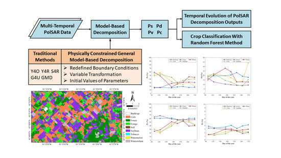
Crop Classification Based on the Physically Constrained General Model-Based Decomposition Using Multi-Temporal RADARSAT-2 Data

Abstract

Crop identification and classification are of great significance to agricultural land use management. The physically constrained general model-based decomposition (PCGMD) has proven to be a promising method in comparison with the typical four-component decomposition methods in scattering mechanism interpretation and identifying vegetation types. However, the robustness of PCGMD requires further investigation from the perspective of final applications. This paper aims to validate the efficiency of the PCGMD method on crop classification for the first time. Seven C-band time-series RADARSAT-2 images were exploited, covering the entire growing season over an agricultural region near London, Ontario, Canada. Firstly, the response and temporal evolution of the four scattering components obtained by PCGMD were analyzed. Then, a forward selection approach was applied to achieve the highest classification accuracy by searching an optimum combination of multi-temporal SAR data with the random forest (RF) algorithm. For comparison, the general model-based decomposition method (GMD), the original and its three improved Yamaguchi four-component decomposition approaches (Y4O, Y4R, S4R, G4U), were used in all tests. The results reveal that the PCGMD method is highly sensitive to seasonal crop changes and matches well with the real physical characteristics of the crops. Among all test methods used, the PCGMD method using six images obtained the optimum classification performance, reaching an overall accuracy of 91.83%.

1. Introduction

The spatial distribution information of crops is essential for farm management and government decision-making [1,2]. Traditional field surveys are time-consuming and labor-intensive, making it difficult to meet the requirements of large-scale operational monitoring [3]. Compared with optical sensors, synthetic aperture radar (SAR) sensors are not affected by cloud, fog, and light rain, and they can acquire ground information during the day and at night. Moreover, measured backscattering shows high sensitivity to the vertical structure and dielectric constant of vegetation, hence it can be used as an effective means for crop identification and classification. In addition, due to dynamic evolution during crop growth, the geometric structure and physical property of crops at different growth stages exhibit significant differences [4,5]. Therefore, time-series SAR images acquired throughout the growing season have been increasingly used for crop classification with promising results [6,7,8,9,10].

Polarimetry is the inherent vector characteristic of electromagnetic waves. SAR polarization exploits the polarization state of radar electromagnetic waves in applications, and is sensitive to the shape structure, orientation, and dielectric properties of the targets [2]. The fully polarimetric synthetic aperture radar (PolSAR), adding observations in the polarimetric dimension, can acquire rich information from the interaction between ground objects and SAR waves. Based on this, PolSAR decomposition can be employed to separate diverse scattering mechanisms and extract various polarimetric parameters and has been extensively applied for crop classification [11,12]. In general, polarimetric decomposition methods with use in natural scenarios (i.e., polarimetric incoherent decomposition) exploiting the covariance/coherency matrix of the second-order statistics, can be generally attributed into three categories, i.e., the Huynen-type phenomenological dichotomy, the eigenvalue–eigenvector-based decomposition, and the model-based decomposition [13,14,15,16,17]. The last one, first introduced by Freeman and Durden [18], describes the backscattering contributions from the ground, the ground and trunk interaction, and the top of the vegetation canopy, respectively. Due to its clear physical meaning and simplicity of calculation, it has been widely used in scattering mechanism interpretation and land-cover classification over vegetated areas.

The traditional Freeman–Durden three-component decomposition method assumed that the canopy consists of dipoles obeying uniform distribution, and its cross-polarization terms are zero in surface and double-bounce scattering models [18]. In practical applications, however, highly oriented built-up areas generate strong scattering power in cross-polarization and are mistaken as strong volume scattering, hence overestimating the contribution of volume scattering. In model parameter calculation, the observed matrix is first subtracted by the volume scattering component, which implies the assumption of model priority. In this vein, the negative power of surface scattering or double-bounce scattering may occur. Moreover, polarimetric information in the observed matrix has not been used completely, leading to the underdetermined problem in the solution of the model. To deal with it, the branch conditions have to be set in the solution process. The above deficiencies limit the applicability of the traditional model-based decomposition methods in many scenarios and spark broad interest in the research community [19,20,21,22,23,24,25,26,27].

In past decades, a variety of modifications have been proposed to further improve model-based decompositions. For example, Yamaguchi et al. [19] proposed a four-component decomposition (Y4O) approach to represent the reflection asymmetry case by introducing the helix scattering component. In addition, two probability density functions were proposed to construct two types of volume scattering matrix corresponding to horizontal and vertical dipoles models. Later, a series of Yamaguchi-based four-component decomposition methods by considering the rotation of polarimetric orientation angle (e.g., Y4R [20], S4R [21], and G4U [22]), or adding more physical scattering models to describe other scattering components (e.g., five-component [23], six-component [24], and seven-component [25,26] decomposition methods) were proposed to reduce the effects caused by overestimation of volume scattering and negative powers. From a mathematic viewpoint, Van Zyl et al. [27] introduced the non-negative eigenvalue decomposition, which requires that all eigenvalues of the covariance matrix are non-negative to overcome the problem of negative powers. In addition, some generalized volume scattering models using a continuous range of shape and scattering randomness to characterize complex volume scenes were proposed and incorporated into the decomposition framework to achieve better scattering mechanism interpretation over regions with different types of vegetation [28,29,30,31].

Although all the aforementioned methods can improve model performance to a certain extent, most of them only partially addressed the well-known limitations. By incorporating many advances, Chen et al. [32] developed a general model-based decomposition (GMD) approach by considering four kinds of volume scattering models, introducing independent orientation angles into surface and double-bounce scattering models for considering the cross-polarization power. Different from the traditional decomposition models, the nonlinear equations are constructed to solve all polarization parameters simultaneously using complete polarization information, which can avoid the assumptions of model inversion priority and the constraints of branch conditions. The experimental results showed superiority over the traditional decomposition methods. However, the accuracy of nonlinear solutions often depends on the selection of initial values and boundary conditions of model parameters. Regarding these issues, Xie et al. [33] further proposed a physically constrained general model-based decomposition (PCGMD) method, which redefined the initial values and boundaries of model parameters by taking account of a popular physical range for dielectric constant, and introduced a variable transformation to make the inversion easier. Later on, several modified PCGMD methods were proposed by further considering several generalized volume scattering models [34,35]. The results indicate that the PCGMD methods produce more reasonable results in scattering mechanism interpretation and outperform the traditional methods. Moreover, physically constrained boundaries contribute more than the other two modifications to improve the decomposition result [33]. Unfortunately, the ground truth is unknown in practice; directly and quantitatively validating the performance of polarimetric decomposition methods is still a tough task. While the Monte Carlo simulation tests designed for different scattering scenes were used in [33,34,35], the current method for evaluating polarimetric decomposition method is mainly limited to scattering power analysis of different scattering components over various land cover types and to make some physical explanations according to theoretical expectations. However, users are more interested in choosing the proper polarimetric decomposition method in practice. Therefore, the performance of the PCGMD method needs to be further investigated from the perspective of final applications.

Regarding this issue, this paper aims to validate the efficiency of the PCGMD method on crop classification employing time-series PolSAR data across the entire growing season. The selected study area was an agricultural area in southwestern Ontario, Canada. Seven C-band RADARSAT-2 images were acquired across the entire growth period of major crops. The responses of the PCGMD method to seasonal crop changes were analyzed, and the application potential of the method for crop classification was evaluated by employing the random forest (RF) algorithm.

Although multi-temporal SAR data containing the structural and physical parameters change information covering the crops growing cycle can improve the classification accuracy, it does not mean that the more images involved in the classification, the higher the accuracy of classification [36,37,38]. The accuracy may reach saturation even worse because the added SAR image at a certain date may not further increase the difference between crops, but increase the similarity of some crops. Previous studies suggested that a combination of images acquired on critical dates during the peak biomass stage and autumn periods may provide even better crop classification accuracy [3,38]. Consequently, we adopted a forward selection procedure recently proposed in [3] by selecting image set for classification iteratively with a step of one image to achieve the highest classification accuracy. The optimal image subset giving the highest classification accuracy was selected in the previous round and kept as the start point in the next round.

This paper is organized as follows. Section 2 introduces the image dataset and ground measurements. Section 3 reviews the original GMD method and introduces the PCGMD algorithm, followed by a brief introduction of the classification method in experiments. In Section 4, the results of six PolSAR decomposition methods and crop classification results based on decomposition scattering powers are presented. In Section 5, a discussion and insights from the results of temporal evolution and classification are given. Finally, the conclusion is drawn in Section 6.

2. Study Area and Dataset

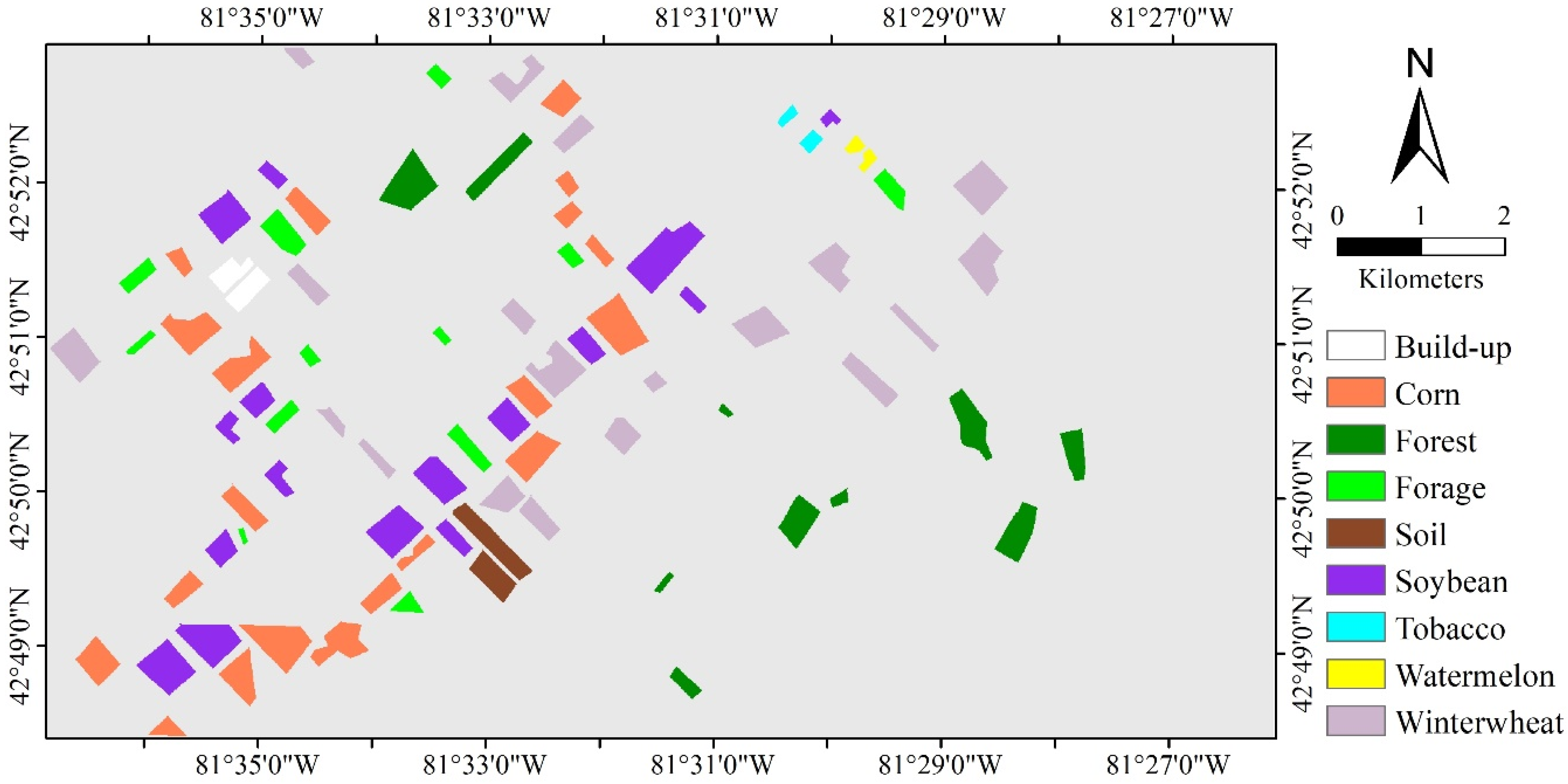
2.1. Study Area and PolSAR Data

In this paper, the test site is located in an agricultural area near London, Ontario, Canada. The Pauli RGB image on 27 September 2015 and the optical image from Google Earth on 23 October 2015 overlaying our study site are presented in Figure 1. The topography of this area is flat. The area experiences a temperate continental humid climate with moderate temperature and abundant rainfall, which is very suitable for agricultural production. The main land cover types are crops, forests, and a few built-up areas. The main crop types are corn, soybean, winter wheat, and forage, and a small amount of tobacco and watermelon also exist on the site.

Generally, winter wheat in this area is planted in October of the former year, and the harvest time is July of the current year. In contrast, the seeding time of corn and soybean is May, and the harvest time is around October in the same year. Due to the crop rotation mechanism in this region, different crop types will be planted after the harvest in October. For the purpose of crop classification using multi-temporal data across the growing season, seven FQ10W (fine quad-pol wide) RADARSAT-2 data obtained between April and September in 2015 were selected in this paper. Detailed information of the SAR dataset is listed in

Table 1. Description of RADARSAT-2 dataset.

Acquisition Date	Mode	Incidence	Resolution	Orbit	Look Direction
12 April 2015	FQ10W	28.4–31.6°	5.5 m × 4.7 m	Ascending	Right
6 May 2015	FQ10W	28.4–31.6°	5.5 m × 4.7 m	Ascending	Right
23 June 2015	FQ10W	28.4–31.6°	5.5 m × 4.7 m	Ascending	Right
17 July 2015	FQ10W	28.4–31.6°	5.5 m × 4.7 m	Ascending	Right
10 August 2015	FQ10W	28.4–31.6°	5.5 m × 4.7 m	Ascending	Right
3 September 2015	FQ10W	28.4–31.6°	5.5 m × 4.7 m	Ascending	Right
27 September 2015	FQ10W	28.4–31.6°	5.5 m × 4.7 m	Ascending	Right

. All images share the same observation mode, incidence angle, and pixel resolution.

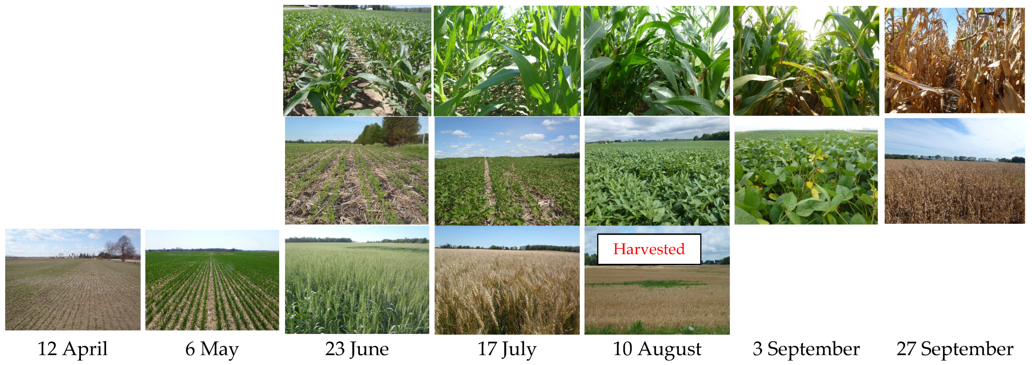
2.2. Ground Truth Data

During the crop growth cycle from April to September 2015, we conducted intensive fieldwork and collected ground measurements. Figure 2 shows crop photos at key growth stages corresponding to the SAR image acquisition dates (exact or closest). No ground photos for corn and soybean were taken on 12 April and 6 May because they had not emerged yet. It should be noticed that wheat straws from the current year’s winter wheat harvest can be seen in the photo in Figure 2. Therefore, only one field survey of winter wheat fields was taken during the harvest, on 10 August. After inspecting the field photos shown in Figure 2, it is expected that the acquired time-series PolSAR images reflect the morphological and structural changes throughout the crop growing season.

According to field surveys, the land cover types of 85 fields were identified, and the spatial distribution is shown in Figure 3. Through random selection at the field level, all the fields were divided into two groups without overlap, with one group of the fields used for training the classifiers and the other for testing.

Table 2. Training and testing samples for crop classification.

Land Cover	Training Samples		Testing Samples
	Number of Pixels	Number of Fields	Number of Pixels	Number of Fields
Corn	6257	4	20,246	16
Soybean	6505	4	15,995	12
Forage	3700	5	3615	7
Winter wheat	6018	3	17,723	16
Watermelon	310	1	309	1
Tobacco	416	1	301	1
Forest	5148	4	7292	6
Built-up	1267	1	1117	1
Soil	2331	1	1592	1

shows the detailed statistics of pixels for training and testing.

3. Methodology

3.1. General Model-Based Decomposition (GMD)

The GMD method proposed by Chen et al. [32] considers four types of physical scattering models of the scene.

3.1.1. Surface Scattering Model

The basic surface scattering model is the well-known Bragg model, which simulates the scattering from a slightly rough surface and ignores the cross-polarization component. The coherency matrix is expressed as [14]:

$$T_s=f_s\left[\begin{array}{ccc}1& {\beta }^{*}& 0\\ \beta & |\beta {|}^2& 0\\ 0& 0& 0\end{array}\right]$$

(1)

where $\beta$ is related to the Bragg reflection coefficients and is expressed as:

$$\beta =\frac{R_H-R_V}{R_H+R_V}$$

(2)

The two coefficients ($R_H, R_V$) are functions of the local incidence angle $\theta$ and the relative dielectric constant of the rough surface ${\epsilon }_S$, which are defined as:

$$R_H=\frac{cos\theta -\sqrt{{\epsilon }_S-si{n}^2\theta }}{cos\theta +\sqrt{{\epsilon }_S-si{n}^2\theta }}$$

(3)

$$R_V=\frac{\left({\epsilon }_S-1\right)\left(si{n}^2\theta -{\epsilon }_S\left(1+si{n}^2\theta \right)\right)}{{\left({\epsilon }_{S}cos\theta +\sqrt{{\epsilon }_S-si{n}^2\theta }\right)}^2}$$

(4)

The imaginary part of ${\epsilon }_S$ can be ignored for most natural scenes in model inversions, and thus $\beta$ is approximately considered to be a real value instead of a theoretical complex value. In the GMD algorithm, Chen et al. [32] introduced a rotation angle ${\theta }_s$ to represent the cross-polarization component caused by terrain slopes [39]. The modified general surface scattering model is written as:

$$T_s\left({\theta }_s\right)=R_3\left({\theta }_s\right)T_s{R}_3^H\left({\theta }_s\right)$$

(5)

$$R_3\left({\theta }_s\right)=\left[\begin{array}{ccc}1& 0& 0\\ 0& cos2{\theta }_s& sin2{\theta }_s\\ 0& -sin2{\theta }_s& cos2{\theta }_s\end{array}\right]$$

(6)

where $R_3^H\left({\theta }_s\right)$ is the conjugate transpose of $R_3\left({\theta }_s\right)$.

3.1.2. Double-Bounce Scattering Model

In general, the double-bounce scattering mechanism is modeled to simulate the scattering from ground-trunk or ground-wall by a dihedral corner formed by two perpendicular reflector surfaces with different dielectric properties. The corresponding coherence matrix has the form:

$$T_d=f_d\left[\begin{array}{ccc}|\alpha {|}^2& \alpha & 0\\ {\alpha }^{*}& 1& 0\\ 0& 0& 0\end{array}\right]$$

(7)

where the value of $\alpha$ is determined by two aspects: the Fresnel reflection coefficients ($R_{iH}, R_{iV}$ for horizontal and vertical polarized waves where$i\in \left\{S,T\right\}$ represents surface and vertical surface, respectively), and the phase difference $\varphi$ between co-polarization channels, which may be affected by different attenuations during the radar wave propagation. It is expressed as:

$$\alpha =\frac{R_{TH}{R}_{SH}+e^{j\varphi }{R}_{TV}{R}_{SV}}{R_{TH}{R}_{SH}-e^{j\varphi }{R}_{TV}{R}_{SV}}$$

(8)

$$R_{iH}=\frac{\mathit{cos}{\theta }_i-\sqrt{{\epsilon }_i-{\mathit{sin}}^2{\theta }_i}}{\mathit{cos}{\theta }_i+\sqrt{{\epsilon }_i-{\mathit{sin}}^2{\theta }_i}}$$

(9)

$$R_{iV}=\frac{{\epsilon }_i\mathit{cos}{\theta }_i-\sqrt{{\epsilon }_i-{\mathit{sin}}^2{\theta }_i}}{{\epsilon }_i\mathit{cos}{\theta }_i+\sqrt{{\epsilon }_i-{\mathit{sin}}^2{\theta }_i}}$$

(10)

where ${\epsilon }_i$ represents the dielectric constant, and ${\theta }_i$ $({\theta }_T=\pi /2-{\theta }_S$) describes the incidence angles for surface and vertical planes. Similarly, a rotation angle is also used to simulate the effect caused by oriented build-up in the double-bounce scattering model and the final expression is:

$$T_d\left({\theta }_d\right)=R_3\left({\theta }_d\right)T_d{R}_3^H\left({\theta }_d\right)$$

(11)

$$R_3\left({\theta }_d\right)=\left[\begin{array}{ccc}1& 0& 0\\ 0& cos2{\theta }_d& sin2{\theta }_d\\ 0& -sin2{\theta }_d& cos2{\theta }_d\end{array}\right]$$

(12)

3.1.3. Volume Scattering Model

Volume scattering from vegetation canopy is generally described as a cloud of uniformly distributed and randomly oriented particles. Assuming the coherency matrix of a single particle is $T\left(\theta \right)$, the coherence matrix of volume scattering is described by integrating over the probability density function of the orientation angle $p\left(\theta \right)$ within a specific range, which can be expressed as:

$$T_v={{\displaystyle \int }}_0^{2\pi }T\left(\theta \right)p\left(\theta \right)d\theta =\left[\begin{array}{ccc}a& d& e\\ d^{*}& b& f\\ e^{*}& f^{*}& c\end{array}\right]$$

(13)

The GMD method considers four commonly used volume scattering models, which are: the Freeman–Durden volume scattering model [18] following a uniform angular distribution width, two Yamaguchi volume scattering models obeying sine and cosine distributions [19], and the maximum entropy model proposed by An et al. [40,41]. Their expressions can be written as:

$$T_{\mathit{vol-random}}=\frac{f_v}{4}\left[\begin{array}{ccc}2& 0& 0\\ 0& 1& 0\\ 0& 0& 1\end{array}\right]$$

(14)

$$T_{\mathit{vol-entropy}}=\frac{f_v}{3}\left[\begin{array}{ccc}1& 0& 0\\ 0& 1& 0\\ 0& 0& 1\end{array}\right]$$

(15)

$$T_{\mathit{vol-horizontal}}=\frac{f_v}{30}\left[\begin{array}{ccc}15& 5& 0\\ 5& 7& 0\\ 0& 0& 8\end{array}\right]$$

(16)

$$T_{\mathit{vol-vertical}}=\frac{f_v}{30}\left[\begin{array}{ccc}15& -5& 0\\ -5& 7& 0\\ 0& 0& 8\end{array}\right]$$

(17)

3.1.4. Helix Scattering Model

The helix scattering model is proposed to describe the situation when the assumption of reflection symmetry is not valid [19]. The corresponding coherence matrix is rotation invariable, and its form is given as [42]:

$$T_c=\frac{1}{2}\left[\begin{array}{ccc}0& 0& 0\\ 0& 1& \pm j\\ 0& \mp j& 1\end{array}\right]$$

(18)

where $j$ represents pure imaginary number.

3.1.5. Model Parameters Inversion

According to the GMD method [32], the observed coherency matrix is given as:

$$T=T_s\left({\theta }_s\right)+T_d\left({\theta }_d\right)+T_v+T_c+T_{residual}$$

(19)

where $T_{residual}$ is the residual matrix, indicating the difference between the model and observations.

Since $T$ is a Hermitian matrix, it can provide nine real-valued observations at most. There are also nine unknowns in the GMD model ($f_s,f_d,f_v,f_c,Re\left[\alpha \right],Im\left[\alpha \right],\beta ,{\theta }_s, {\theta }_d$). To invert this model, nine nonlinear equations are constructed, and parameters are solved based on the criterion of the minimization of residuals. This optimization criterion is expressed as:

$$min:\Vert T_{residual}\Vert {}_2^2$$

(20)

In addition, Chen et al. [32] choose the outputs obtained from the Y4O method as the initial values of the major parameters ($f_s,f_d,f_v,f_c,Re\left[\alpha \right],Im\left[\alpha \right],\beta$) in the nonlinear optimization algorithm. The initial values of ${\theta }_s$ and ${\theta }_d$ are the negative values of the polarization orientation angle. Also, the boundary conditions of parameters are set as:

$$\begin{array}{c}0\le f_v,f_s,f_d\le SPAN 0\le f_c\le 2\left|\mathrm{Im}\left(T_{23}\right)\right|\\ -\frac{\pi }{4}\le {\theta }_s,{\theta }_d\le \frac{\pi }{4}\left|\beta \right|,\left|\alpha \right|<1\end{array}$$

(21)

where SPAN is the total power.

3.2. Physically Constrained General Model-Based Decomposition (PCGMD)

Although the GMD method proposed by Chen et al. [32] offers multiple advantages, the process for solving the final parameters depends on nonlinear optimization algorithms, which may face the issues of local optimal solutions and even physically unfeasible solutions. These issues are mainly caused by inaccurate initial value selection and unreasonable parameter boundary setting. To address these issues, without changing the original GMD framework, the PCGMD approach was further developed by Xie et al. [33] which includes three modifications (The matlab code of PCGMD is available at https://www.researchgate.net/publication/315657548_Matlab_implementation_of_a_general_model-based_decomposition_for_PolSAR_data, (accessed on 29 May 2022)).

3.2.1. Redefined Boundary Conditions

From Equations (3), (4), (9) and (10), it is clear that parameters $\alpha$ and $\beta$ are related to incidence angle and relative dielectric constants. The value of α depends on the polarization phase difference $\varphi ,$ with a range of $\left[-\pi , \pi \right]$. Therefore, in theory, all possible values of $\alpha$ and $\beta$ can be calculated using the given incidence angle and phase difference over a particular range of dielectric constants, and the maximum and minimum values can be found as the basis for redefining the upper and lower boundaries, respectively. Previous studies have shown that the relative dielectric constant has a certain physical range for most natural scenarios [43]. A frequently used and wide enough empirical physical range of $\epsilon$ is [2,41,44,45].

By setting the physical ranges and incidence angle, an analysis of values of unknown parameters in the decomposition model was conducted using numeric simulation experiments [33]. The results showed that it is difficult to obtain the boundary of $Re\left[\alpha \right]$and$Im\left[\alpha \right]$ according to the existing conditions, hence these two unknown parameters are equivalently replaced by the magnitude $\left|\alpha \right|$ and the argument $\arg \left(\alpha \right)$. The boundaries of $\left|\alpha \right|$ and $\arg \left(\alpha \right)$ are obviously dependent on the phase difference $\varphi$, which is unknown in practice and, consequently, some assumptions must be made. As it is known, the physical meaning of the Pauli decomposition shows that the scattering mechanisms dominated by surface scattering and double-bounce scattering are corresponding to $HH+VV$ and $HH-VV$ polarization modes, respectively. It assumes for the double-bounce contribution that the power of $HH+VV$ is less than that of $HH-VV$, which is equivalent to say that $T_{11}$ is less than $T_{22}$ in the coherence matrix $T_d$. Combined with Equation (7), the upper boundary condition of $\left|\alpha \right|$ is expressed as $\left|\alpha \right|<1$, and the value of $\varphi$ will be automatically constrained. Based on the above analysis, for any pixel $i$, the boundary conditions of parameter $\alpha$ are redefined as:

$$|\alpha {|}_{min}\left\{\varphi =0,\theta ={\theta }_i\right\}<\left|\alpha \right|<1$$

(22)

$$\mathrm{Arg}{(\alpha )}_{min}\left\{\varphi ={90}^{\circ },\theta ={\theta }_i\right\}<\arg \left(\alpha \right)<\mathrm{Arg}{(\alpha )}_{max}\left\{\varphi =-{90}^{\circ },\theta ={\theta }_i\right\}$$

(23)

Similarly, the boundary conditions of parameter $\beta$ are redefined as:

$${\beta }_{min}\left\{\theta ={\theta }_i\right\}\le \beta \le {\beta }_{max}\left\{\theta ={\theta }_i\right\}$$

(24)

Furthermore, the powers of scattering components are smaller than the total power $SPAN$ and are non-negative. The boundaries have the following expressions:

$$0\le P_s=f_s\left(1+|\beta {|}^2\right)\le SPAN$$

(25)

$$0\le P_d=f_d\left(1+|\alpha {|}^2\right)\le SPAN$$

(26)

They are two additional inequality conditions among parameters. In order to simplify the process of parameter inversion, the boundary conditions of these two parameters are properly relaxed, and the obtained boundary conditions are expressed as:

$$0\le f_s\le \frac{SPAN}{\left(1+|\beta {|}_{min}^2\right)} 0\le f_d\le \frac{SPAN}{\left(1+|\alpha {|}_{min}^2\right)}$$

(27)

In summary, the PCGMD algorithm redefines the following parameters: (a) the lower boundary of $\left|\alpha \right|$; (b) the upper and lower boundaries of $\arg \left(\alpha \right)$; (c) the upper boundary and lower boundary of $\beta$; (d) the upper and lower boundaries of $f_s$ and $f_d$. For any pixel, the redefined boundaries adaptively change with the incidence angle.

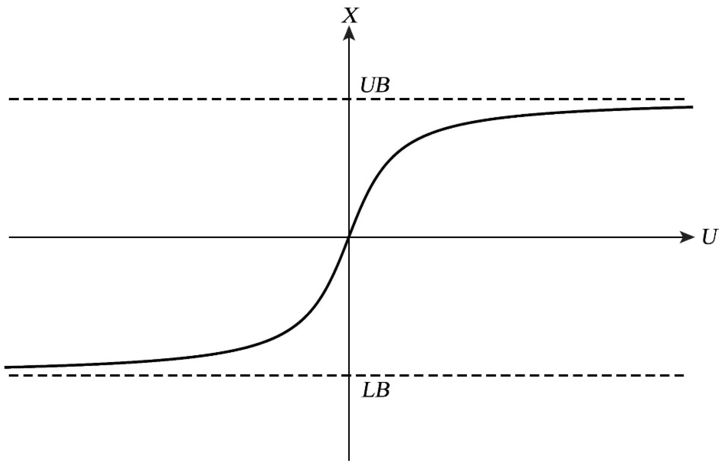
3.2.2. Variable Transformation

The idea of variable transformation can be used to transform the constrained variables into unconstrained variables for nonlinear least-square optimization. For example, for variable $X$, we can make a change of variable using the inverse tangent function based on the boundary conditions. The transformation can be written as:

$$X=LB+\left(UB-LB\right)\times \frac{\mathrm{atan}\left(U\right)+\frac{\pi }{2}}{\pi }$$

(28)

where $UB$ and $LB$ are the upper and lower bounds of parameter $X$, respectively. The relationship between the transformed variable and the original one is illustrated in Figure 4. The value of the new variable $U$ is unrestricted, which makes the range of all parameters consistent and the solution process easier. As the transformation is substituted into the objective function of the parameter, the solution of the model parameters becomes an unconstrained optimization problem dependent on variable $U$.

3.2.3. Initial Values of Parameters

The GMD algorithm uses the outputs obtained from the traditional Yamaguchi four-component decomposition as the initial values of parameters [32]. However, the traditional decomposition method meets an underdetermined problem (i.e., unknowns are more than observations) in the last step of parameter solving. It needs to fix parameter $\alpha$ or $\beta$ to get the values of $f_s$ and $f_d$ under branching conditions, which may lead to wrong solutions, i.e., beyond reasonable physical boundaries. In order to solve this problem, the initial values of $\alpha$ and $\beta$ can be set as middle values of their physical boundaries. The final step in common three or four component model-based decomposition methods for solving $\alpha$, $\beta$, $f_s,$ and $f_d$ is an undetermined problem because unknowns are more than equations [22]. Since $\alpha$ and $\beta$ are redefined and already known, it becomes an overdetermined problem [33]. The initial values of $f_s$ and fd are thereby set from the least-squares solutions based on the redefined initial values of $\alpha$ and $\beta$. The initial values of the remaining parameters are the same as the original GMD method.

3.3. Classification Method

In this paper, the efficiency of PolSAR decomposition methods for crop classification was evaluated using the random forest (RF) [46] classifier. The RF algorithm can generate a number of decision trees by randomly selecting $N$ sample units out of the training samples with replacement, which is an ensemble learning method. It not only produces good accuracy but can also assess the importance of each feature’s contribution to the classification. Due to its advantages, it has been popular in crop classification using SAR data [47,48,49]. Previous studies show that the accuracy of crop classification tends to be stable as the decision trees exceed 50 [48,50]. The number of RF decision trees in this study was set to 100.

By applying four-component polarization decompositions, four scattering component parameters (Ps, Pd, Pv, Pc) were obtained for each image. Usually, a combination of all images is adopted in crop classification with time-series data. For example, a total of 28 scattering component parameters from each decomposition method can be merged as the input features for crop classification. However, previous investigations also show that combining selected images acquired on critical dates may provide comparable or even better classification accuracy [36,37,38]. Furthermore, it can reduce the cost due to image purchase and processing burden for users.

Recently, Li et al. [3] proposed a forward image selection algorithm to achieve the highest classification accuracy by searching the optimal set of SAR images. In this algorithm, the images were iteratively chosen to construct the image set (starting from null) for classification by adding one image along the SAR acquisition time. For example, a single image along the SAR acquisition time obtaining the highest classification accuracy will be chosen in the first round and set as the basic image set in the second round. By adding images gradually, we can finally obtain the image combination with the best accuracy among all combinations of images. This approach has also been exploited in this work.

4. Results

4.1. PolSAR Decomposition Results

After a series of PolSAR data preprocessing steps, the time-series RADARSAT-2 images were transformed to multi-temporal geocoded coherency matrices. Then, six types of the four-component decomposition methods were applied to produce the scattering powers (i.e., Ps, Pd, Pv, Pc). For comparison, besides the GMD and PCGMD methods, the Y4O, Y4R, S4R, and G4U were tested as well.

By calculating the scattering contributions over all fields with the same land-cover type, the temporal evolutions of the resulting four scattering power parameters from six polarimetric decomposition methods were obtained. The series measuring built-up areas, forests, and three main crops are given in Figure 5. The results show that Yamaguchi modifications (i.e., Y4R, S4R, G4U) reveal similar patterns with reduced volume scattering overestimation compared with the original Yamaguchi method (Y4O). Therefore, the latter analysis does not emphasize the differences among Yamaguchi modifications. In detail, the double-bounce scattering is not dominant as expected over the built-up area, and the volume scattering mechanism is dominant using all six decomposition methods. From the optical image in Figure 1 and the ground survey map shown in Figure 3, we found that the built-up area in this site is actually a small power station consisting of open concrete ground and some electric power facilities with ordered arrangement. This kind of structure may generate volume scattering. However, it can still be found that the GMD and PCGMD methods have lower volume scattering power compared to the traditional methods. Moreover, the PCGMD shows the largest double-bounce scattering contribution, which is in line with the common interpretation of radar scattering in built-up areas.

In forest area, as expected, volume scattering is dominant in all decomposition models. With respect to the Y4O method, Yamaguchi modifications can significantly reduce the volume scattering overestimation, but it is still on the high side. Compared with Yamaguchi modifications, both GMD and PCGMD show higher double-bounce scattering, which somehow reflects the vertical structure of forest-covered areas.

Over crop areas, the contributions of double-bounce scattering using GMD and PCGMD methods are higher than those using traditional decomposition methods. Since the planting and harvesting dates of corn and soybean are roughly the same, the scattering mechanisms have the same changing trend: they are dominated by surface scattering and then gradually change to volume scattering. However, the double-bounce scattering component increases significantly on the last date due to the presence of crop residues after harvest, especially over corn fields. For winter wheat, volume scattering is the dominant scattering mechanism only during the vigorous growth stage from June to August, and it decreases gradually until right before harvest.

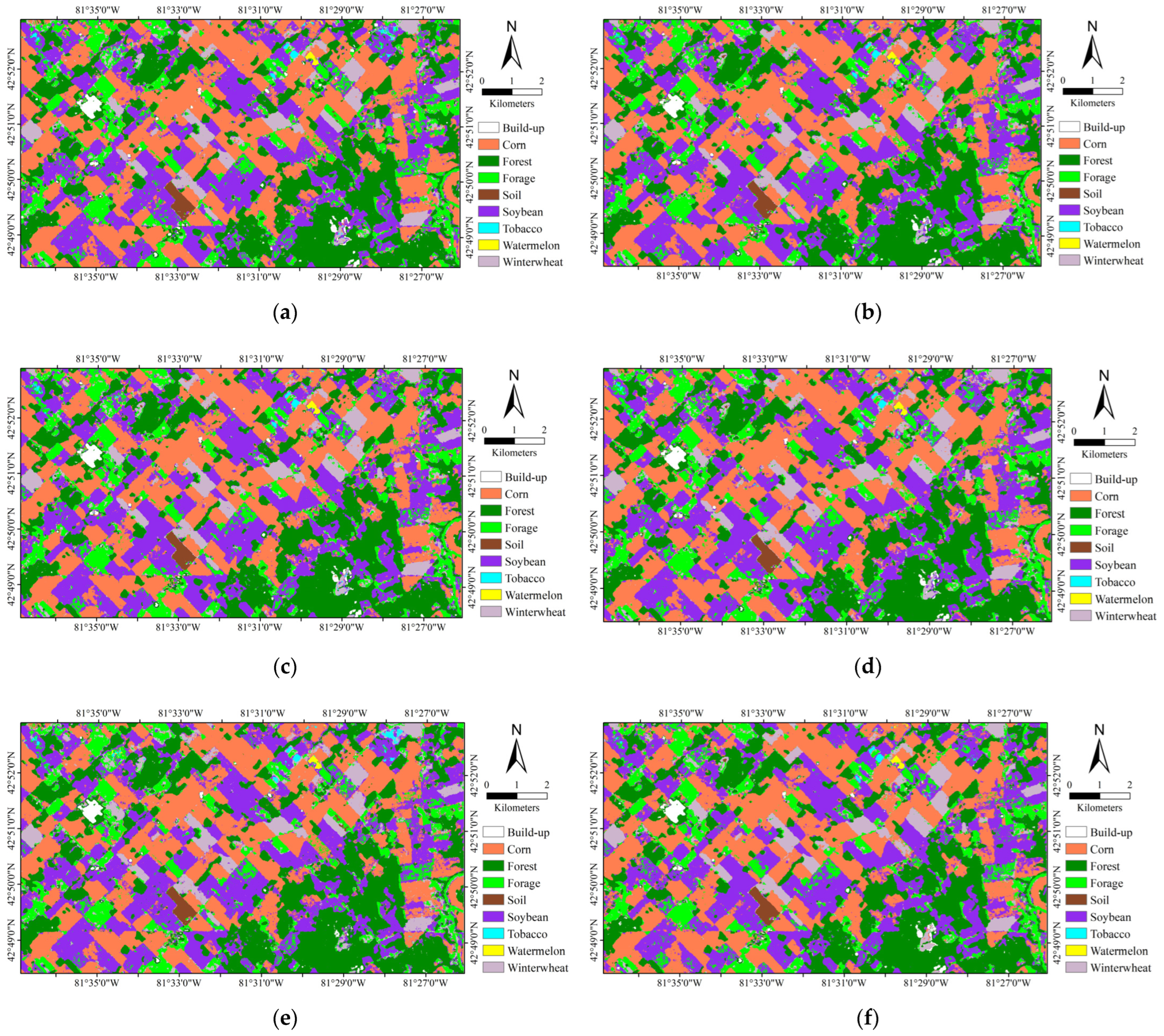
4.2. Crop Classification Results

As depicted in Figure 6, in case of a single image for classification, the image in June produced the best overall accuracy (OA) using the four traditional Yamaguchi methods (Y4O, Y4R, S4R, G4U), whereas the image in early September was selected for the two general decomposition methods (GMD and PCGMD) with the highest value of OA. Also, it should be noted that all but the GMD reached OAs of 65–68% using a single image.

As more images were added, the classification accuracy gradually improved until it reached saturation. It is interesting to see that using all images does not produce the optimal accuracy in all decomposition methods. Six images produced the best results for Y4O, GMD, and PCGMD, while five images achieved the best accuracy for Y4R, S4R, and G4U. The images acquired on 6 May, 23 June, 10 August, and 3 September are selected in the optimal combination of images for all six polarimetric decomposition methods. Finally, the optimal classification OAs of all six decomposition methods are 89.57% (Y4O), 89.83% (Y4R), 89.71% (S4R), 89.96% (G4U), 88.67% (GMD), and 91.83% (PCGMD). The PCGMD shows the best OA in most cases employing a different number of images. Comparing GMD and PCGMD in all seven cases using different numbers of images, the PCGMD always produced better OAs. Finally, it is worth noting that all six methods produced a notable classification improvement (reaching up to 85%) with just three images, which confirms again the expected positive effect of image timing on crop classification performance.

The producer’s and user’s accuracies (i.e., PA and UA), as well as Kappa coefficient and OA for each crop type corresponding to the optimal classification accuracy after the forward image selection procedure are listed in

Table 3. PAs, UAs, OAs and Kappa coefficients corresponding to the optimal crop classification accuracy in different methods.

Crop Type	Y4O		Y4R		S4R		G4U		GMD		PCGMD
	PA	UA	PA	UA	PA	UA	PA	UA	PA	UA	PA	UA
Corn	95.08	85.75	95.13	85.98	95.25	85.30	95.56	86.29	94.71	84.20	96.59	88.28
Forest	99.81	97.39	99.16	98.73	99.23	98.60	99.25	98.50	99.35	96.92	99.30	98.26
Forage	84.98	61.91	86.92	61.13	85.89	62.08	86.58	61.35	85.67	65.56	88.22	67.95
Soil	93.78	100	95.04	100	94.97	100	95.67	100	92.21	100	93.84	99.87
Soybean	95.42	92.34	94.95	93.02	94.99	93.17	94.52	93.34	94.59	89.96	93.07	94.23
Tobacco	55.81	98.25	59.47	94.71	59.47	98.35	61.13	97.35	55.15	98.22	62.79	99.47
Watermelon	76.05	100	72.82	99.56	78.64	99.18	75.40	99.15	74.43	99.57	77.67	100
Wheat	75.14	96.78	76.26	96.88	75.71	96.69	76.54	96.49	73.16	96.65	83.48	97.76
OA	89.57		89.83		89.71		89.96		88.67		91.83
Kappa	86.44		86.79		86.62		86.95		85.26		89.36

. It illustrates that the optimal OAs obtained by the four traditional four-component decomposition methods are similar. Although the three Yamaguchi modifications mitigate the issues in the original Yamaguchi four-component decomposition, they show only a limited contribution in improving crop classification accuracy. The optimal classification accuracy using GMD method is the worst among all the methods, with an OA of 88.67%. Table 3 also shows that, due to their similar temporal evolutions, winter wheat and corn cannot be accurately distinguished, resulting in large omission error of the winter wheat class in GMD method compared with Yamaguchi methods.

In contrast, the classification PAs and UAs from the PCGMD method are generally high for all crops, even for winter wheat and forage that are difficult to distinguish. The final OA is also the highest among all the methods used, reaching 91.83%. To further illustrate the classification results generated by different methods, Figure 7 shows the classified maps corresponding to the optimal classification obtained by the six decomposition algorithms. In general, all the results present a good clustering pattern, especially the results obtained by the PCGMD method. However, it is also apparent that some scattered errors exist in all methods. This is an expected behavior in pixel-based classification. Object-based classification could overcome this issue.

5. Discussion

Some well-known limitations exist for the model-based polarimetric decomposition method, such as model inversion priority, branch conditions, deorientation effect, negative powers, and incomplete polarimetric information utilization [51]. By incorporating many advances in previous studies, the GMD in [32] mitigated these issues. However, the full-parameter inversion scheme in this method relies on solving nine unknowns from nine nonlinear equations, which is affected by the selection of initial values and boundary conditions of model parameters. It probably leads to physically incorrect decomposition results. To address this issue in parameter solving, without changing the original GMD framework, the physically constrained general model-based decomposition (PCGMD) method was further proposed in [33], which redefined the initial values and boundaries of model parameters incorporating a popular physical range of dielectric constants, and introduced a variable transformation. Due to the lack of ground truth in practice, the performance of PCGMD was evaluated by analyzing the balance among scattering mechanisms over different land cover types according to theoretical expectations as usual and Monte Carlo simulation tests [33,34,35]. However, a direct comparison of final applications based on polarimetric decomposition methods with ground-truth collected simultaneously makes the interpretations more convincing. In this paper, the performance of the PCGMD method and the other five methods (i.e., GMD method and four traditional types of Yamaguchi decomposition methods (Y4O, Y4R, S4R, G4U)) on crop classification using multi-temporal PolSAR data was evaluated. A forward selection approach was applied in the classification procedure to pursue optimal classification accuracy by searching for an optimum combination of multi-temporal SAR images with the random forest (RF) algorithm.

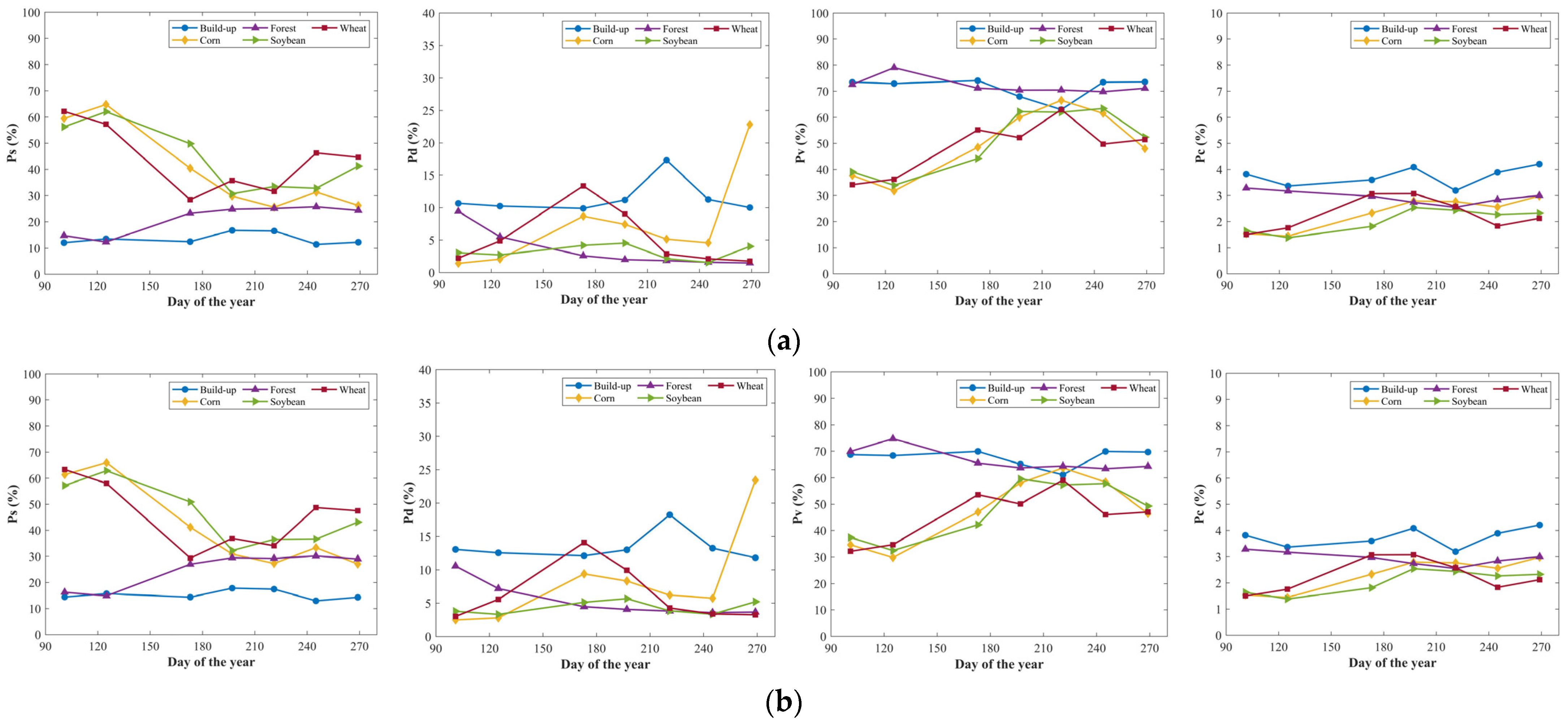
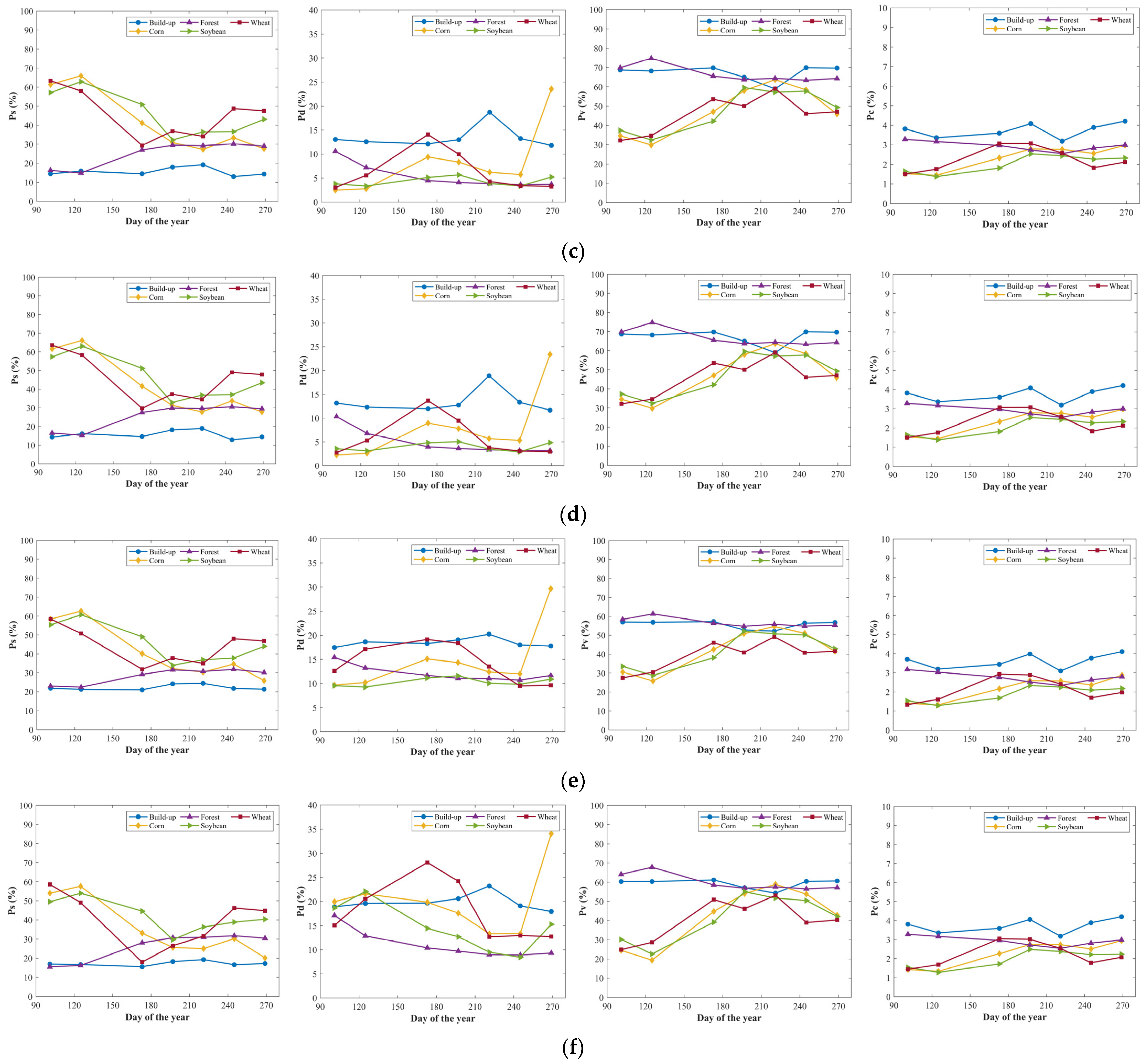
5.1. Temporal Evolution of PolSAR Decomposition Outputs

The results of temporal evolution reveal that the GMD and PCGMD methods produce lower volume scattering power than the traditional Yamaguchi-based decomposition methods over all land cover types, which is consistent with previous results [32,33,34,35]. Although Yamaguchi modifications applied deorientation processing (e.g., Y4R, S4R, G4U) and added volume scattering from oriented dihedral scatter (e.g., S4R, G4U) to reduce overestimation of volume scattering and obtain improvements with respect to original Yamaguchi method (Y4O), misinterpretation still occurs because of the model inversion priority, ignored cross-polarization contributions from surface and double-bounce scattering models, and branch conditions [32]. Besides, the decomposition results also indicate the highly coherent behaviors of Y4R, S4R, and G4U, especially that between S4R and G4U. It can be explained by the fact that our study site is mainly composed of the vegetation area and has no highly oriented buildings, resulting in less volume scattering from dihedral structure, which is in good agreement with decomposition performance in previous studies [22,33]. In contrast, GMD and PCGMD adopt the generalized surface and double-bounce models to account for the cross-polarization power, and use nonlinear equations to solve model parameters at the same time. It can avoid the above limitations and further improved performance is obtained.

Although all six decomposition methods reflect the variation trend as crops grow, Yamaguchi modifications show a relatively lower double-bounce scattering component than the two generalized decomposition methods, which is in line with previous investigations [32,33,34,35]. In addition, PCGMD further shows higher double-bounce scattering than GMD, which somehow indicates the potential of PCGMD in polarimetric SAR urban area classification as the case study in [52].

The dynamic range of scattering mechanism components obtained from the GMD method is the smallest among all methods, whereas the range from the PCGMD method is the largest one. It somehow indicates that the PCGMD method shows the highest sensitivity to the structural changes of crops during their growth. This feature is expected to help applications such as crop monitoring and crop classification.

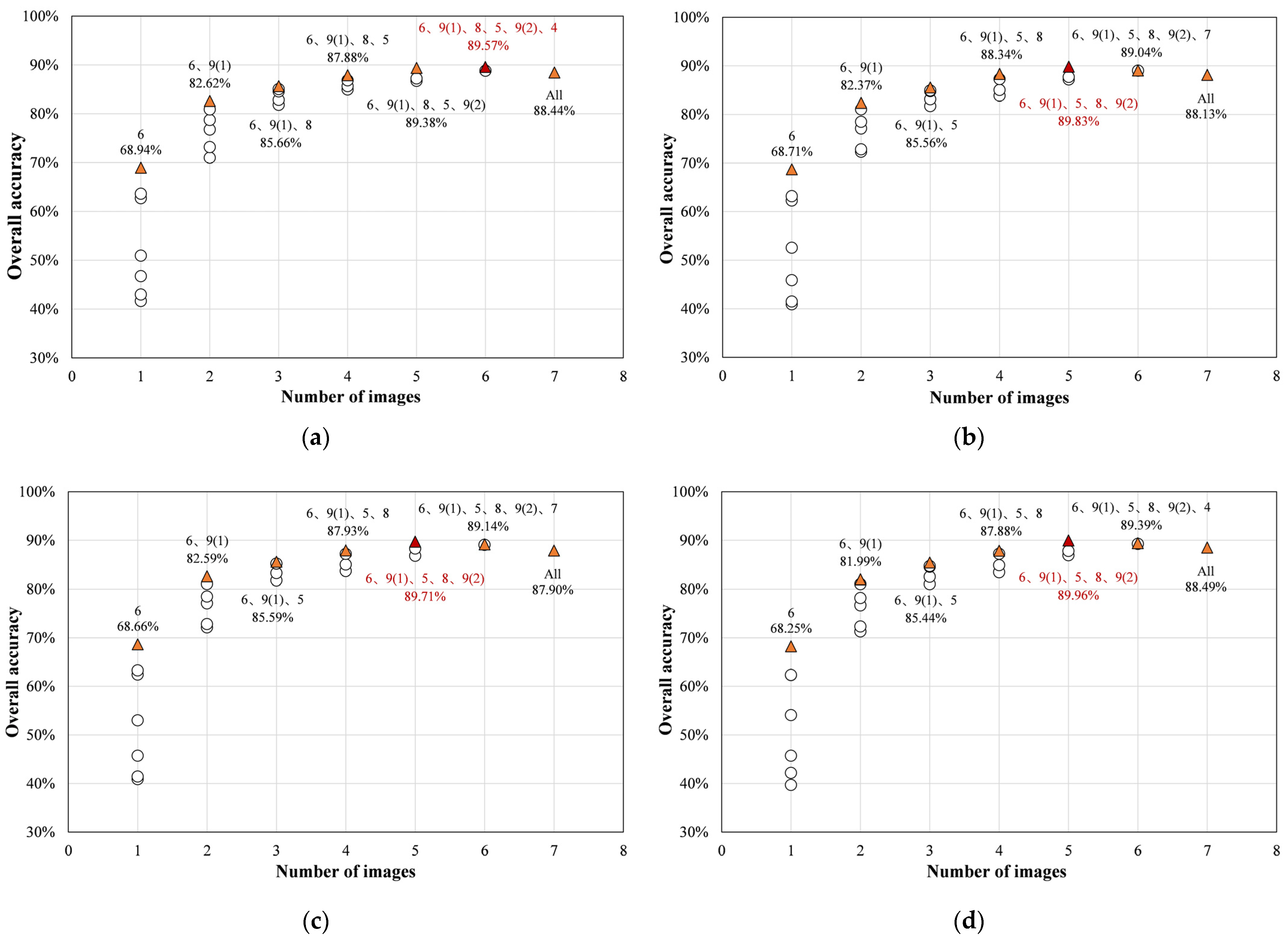
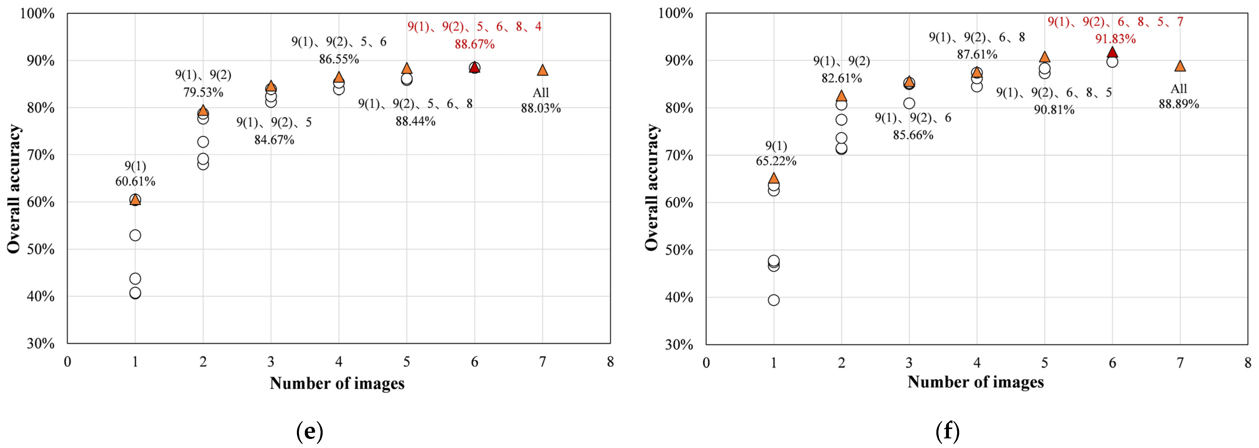
5.2. Crop Classification Accuracy

In the case of a single image for classification, the images in June and September produced the best overall accuracy. The reason may be attributed to the significant differences in growth status and morphological structure of crops in these two periods. According to the field photos in Figure 2, corn and soybean in June were at their early growth stages, and the bare ground can be seen, while winter wheat was at its vigorous stage of growth, and the ground was almost completely covered by leaves. In contrast, the winter wheat was harvested by early September, whereas both corn and soybeans were at the ripening stage and showed apparent differences in height, leaf structure, and moisture content. It somehow shows that the most important images for crop classification are acquisitions dated during the peak biomass stage due to significant structural differences between most crops, which show a similar phenomenon as reported in the previous study [3]. In addition, the results are in line with the study of crop classification in [38] using the same SAR data and ground truth. In [38], using 27 polarimetric observables including three types of decomposition methods, the single image to produce the best overall accuracy was the image from June or September. In the case of multiple images for classification, four images acquired on 6 May, 23 June, 10 August, and 3 September were selected for all methods to produce the best OAs. This illustrates that selected images acquired on critical dates are possible to provide a better classification result as reported in previous studies [3,36,37,38].

Compared with traditional four-component decomposition methods, GMD shows lower OA for crop classification. This result can be explained according to the analysis based on Figure 5. Although the GMD method can inhibit the volume scattering overestimation and improve the contribution from double-bounce scattering, it produces the smallest variation range of the scattering especially for the winter wheat class, leading to poorer separability among classes. The further explanation may be attributed to the numerical variability associated with the non-realistic inversion in the GMD method [33,34]. Although the GMD can enhance the scattering mechanism interpretation performance in urban areas, especially in highly oriented built-up regions as illustrated in the original study [32] and was successfully applicated for urban damage level mapping [53], this study somehow indicates its limitation for the application of crop classification. After considering the physical constraints in PCGMD, the classification performance improved, which shows the best OA of 91.83%. Since the forage type here refers to different morphological structures, such as alfalfa, hay, and grass, it may cause confusion in classification. If the grass is not taken into account in the accuracy calculation, the OA of the PCGMD method would be improved to 94.27%. These results indicate that the modifications involved in the PCGMD model with respect to the GMD method enhance the sensitivity of the decomposition parameters to crop scattering characteristics, which is beneficial to increasing classification performance.

It is noteworthy that all classification methods in this study only rely on the use of the backscattering powers. Additional output features (e.g., $\alpha$ and $\beta$) produced by the decompositions should also be paid attention [33]. The results suggest that the physical constraints added to the original GMD method can not only improve the feasibility of dielectric constant-related parameters, but also the backscattering powers. A complete study of the performance of all outputs from PolSAR decomposition techniques should be investigated. In this vein, further research could emphasize the need of PolSAR decomposition methods to improve parameter retrieval, beyond the mere use of backscattering powers. For example, the performance of the PCGMD method could be further evaluated in other applications, such as soil moisture inversion, urban area classification, and forest type mapping, etc.

6. Conclusions

In this study, a physically constrained general model-based decomposition (PCGMD) method was applied to crop classification for the first time and its performance was evaluated. The GMD method and four traditional types of Yamaguchi decomposition methods (Y4O, Y4R, S4R, G4U) were adopted for comparison. Multi-temporal RADARSAT-2 data across the growing season over a typical agricultural area in southwestern Ontario, Canada, were exploited. Before classification, the temporal evolutions of the scattering components were analyzed. These results indicate that polarimetric decomposition methods can characterize the temporal variations of crop geometric structure and physical characteristics in different classes. The PCGMD method, which retains the original advantages of the GMD method, is more consistent with physical reality and shows higher sensitivity to the temporal evolution of crops. In crop classification tests, based on the random forest classifier, a forward selection procedure was employed to find an optimal image set to achieve the highest classification accuracy. The tests show that the PCGMD produced the best classification accuracy among all six polarimetric decomposition methods, with an OA of 91.83%. Although three Yamaguchi modifications mitigated the problems in the original Yamaguchi four-component decomposition, they produced very limited improvements on crop classification accuracy. Instead, the PCGMD brings apparent improvements, especially with respect to its base method, i.e., the GMD method. It proves again the effectiveness of the modifications included in the PCGMD method. In addition, results from all six methods reveal that using multi-temporal images acquired on critical dates can obtain optimal classification performance.

References

1. Liu, C.; Chen, Z.; Shao, Y.; Chen, J.; Hasi, T.; Pan, H. Research Advances of SAR Remote Sensing for Agriculture Applications: A Review. J. Integr. Agric. 2019, 18, 506–525. [Google Scholar] [CrossRef] [Green Version]
2. McNairn, H.; Shang, J.; Jiao, X.; Champagne, C. The Contribution of ALOS PALSAR Multipolarization and Polarimetric Data to Crop Classification. IEEE Trans. Geosci. Remote Sens. 2009, 47, 3981–3992. [Google Scholar] [CrossRef] [Green Version]
3. Li, H.; Zhang, C.; Zhang, S.; Atkinson, P.M. Crop Classification from Full-Year Fully-Polarimetric L-Band UAVSAR Time-Series Using the Random Forest Algorithm. Int. J. Appl. Earth Obs. Geoinf. 2020, 87, 102032. [Google Scholar] [CrossRef]
4. Liu, C.; Shang, J.; Vachon, P.W.; McNairn, H. Multiyear Crop Monitoring Using Polarimetric RADARSAT-2 Data. IEEE Trans. Geosci. Remote Sens. 2013, 51, 2227–2240. [Google Scholar] [CrossRef]
5. Steele-Dunne, S.C.; McNairn, H.; Monsivais-Huertero, A.; Judge, J.; Liu, P.W.; Papathanassiou, K. Radar Remote Sensing of Agricultural Canopies: A Review. IEEE J. Sel. Top. Appl. Earth Obs. Remote Sens. 2017, 10, 2249–2273. [Google Scholar] [CrossRef] [Green Version]
6. Busquier, M.; Lopez-Sanchez, J.M.; Bargiel, D. Added Value of Coherent Copolar Polarimetry at X-Band for Crop-Type Mapping. IEEE Geosci. Remote Sens. Lett. 2020, 17, 819–823. [Google Scholar] [CrossRef]
7. Huang, X.; Wang, J.; Shang, J.; Liao, C.; Liu, J. Application of Polarization Signature to Land Cover Scattering Mechanism Analysis and Classification Using Multi-Temporal C-Band Polarimetric RADARSAT-2 Imagery. Remote Sens. Environ. 2017, 193, 11–28. [Google Scholar] [CrossRef]
8. Liao, C.; Wang, J.; Xie, Q.; Al Baz, A.; Huang, X.; Shang, J.; He, Y. Synergistic Use of Multi-Temporal RADARSAT-2 and VENμS Data for Crop Classification Based on 1D Convolutional Neural Network. Remote Sens. 2020, 12, 832. [Google Scholar] [CrossRef] [Green Version]
9. Mestre-Quereda, A.; Lopez-Sanchez, J.M.; Vicente-Guijalba, F.; Jacob, A.W.; Engdahl, M.E. Time-Series of Sentinel-1 Interferometric Coherence and Backscatter for Crop-Type Mapping. IEEE J. Sel. Top. Appl. Earth Obs. Remote Sens. 2020, 13, 4070–4084. [Google Scholar] [CrossRef]
10. Xu, L.; Zhang, H.; Wang, C.; Zhang, B.; Liu, M. Crop Classification Based on Temporal Information Using Sentinel-1 SAR Time-Series Data. Remote Sens. 2019, 11, 53. [Google Scholar] [CrossRef] [Green Version]
11. Chen, G.; Wang, L.; Kamruzzaman, M.M. Spectral Classification of Ecological Spatial Polarization SAR Image Based on Target Decomposition Algorithm and Machine Learning. Neural Comput. Appl. 2020, 32, 5449–5460. [Google Scholar] [CrossRef]
12. Xie, Q.; Wang, J.; Liao, C.; Shang, J.; Lopez-Sanchez, J.M.; Fu, H.; Liu, X. On the Use of Neumann Decomposition for Crop Classification Using Multi-Temporal RADARSAt-2 Polarimetric SAR Data. Remote Sens. 2019, 11, 776. [Google Scholar] [CrossRef] [Green Version]
13. Cloude, S.R.; Pottier, E. A Review of Target Decomposition Theorems in Radar Polarimetry. IEEE Trans. Geosci. Remote Sens. 1996, 34, 498–518. [Google Scholar] [CrossRef]
14. Lee, J.S.; Pottier, E. Polarimetric Radar Imaging: From Basics to Applications; CRC Press: Boca Raton, FL, USA, 2009. [Google Scholar]
15. Cloude, S.R. Polarisation: Applications in Remote Sensing; Oxford University Press: New York, NY, USA, 2010. [Google Scholar]
16. Li, D.; Zhang, Y. Adaptive Model-Based Classification of PolSAR Data. IEEE Trans. Geosci. Remote Sens. 2018, 56, 6940–6955. [Google Scholar] [CrossRef]
17. Li, D.; Zhang, Y.; Liang, L. A Mathematical Extension to the General Four-Component Scattering Power Decomposition with Unitary Transformation of Coherency Matrix. IEEE Trans. Geosci. Remote Sens. 2020, 58, 7772–7789. [Google Scholar] [CrossRef]
18. Freeman, A.; Durden, S.L. A Three-Component Scattering Model for Polarimetric SAR Data. IEEE Trans. Geosci. Remote Sens. 1998, 36, 963–973. [Google Scholar] [CrossRef] [Green Version]
19. Yamaguchi, Y.; Moriyama, T.; Ishido, M.; Yamada, H. Four-Component Scattering Model for Polarimetric SAR Image Decomposition. IEEE Trans. Geosci. Remote Sens. 2005, 43, 1699–1706. [Google Scholar] [CrossRef]
20. Yamaguchi, Y.; Sato, A.; Boerner, W.M.; Sato, R.; Yamada, H. Four-Component Scattering Power Decomposition With Rotation of Coherency Matrix. IEEE Trans. Geosci. Remote Sens. 2011, 49, 2251–2258. [Google Scholar] [CrossRef]
21. Sato, A.; Yamaguchi, Y.; Singh, G.; Park, S.E. Four-Component Scattering Power Decomposition with Extended Volume Scattering Model. IEEE Geosci. Remote Sens. Lett. 2012, 9, 166–170. [Google Scholar] [CrossRef]
22. Singh, G.; Yamaguchi, Y.; Park, S.E. General Four-Component Scattering Power Decomposition with Unitary Transformation of Coherency Matrix. IEEE Trans. Geosci. Remote Sens. 2013, 51, 3014–3022. [Google Scholar] [CrossRef]
23. Zhang, L.; Zou, B.; Cai, H.; Zhang, Y. Multiple-Component Scattering Model for Polarimetric SAR Image Decomposition. IEEE Geosci. Remote Sens. Lett. 2008, 5, 603–607. [Google Scholar] [CrossRef]
24. Singh, G.; Yamaguchi, Y. Model-Based Six-Component Scattering Matrix Power Decomposition. IEEE Trans. Geosci. Remote Sens. 2018, 56, 5687–5704. [Google Scholar] [CrossRef]
25. Singh, G.; Malik, R.; Mohanty, S.; Rathore, V.S.; Yamada, K.; Umemura, M.; Yamaguchi, Y. Seven-Component Scattering Power Decomposition of POLSAR Coherency Matrix. IEEE Trans. Geosci. Remote Sens. 2019, 57, 8371–8382. [Google Scholar] [CrossRef]
26. Han, W.; Fu, H.; Zhu, J.; Wang, C.; Xie, Q. Polarimetric SAR Decomposition by Incorporating a Rotated Dihedral Scattering Model. IEEE Geosci. Remote Sens. Lett. 2022, 19, 4–8. [Google Scholar] [CrossRef]
27. Van Zyl, J.J.; Arii, M.; Kim, Y. Model-Based Decomposition of Polarimetric SAR Covariance Matrices Constrained for Nonnegative Eigenvalues. IEEE Trans. Geosci. Remote Sens. 2011, 49, 3452–3459. [Google Scholar] [CrossRef]
28. Antropov, O.; Rauste, Y.; Hame, T. Volume Scattering Modeling in PolSAR Decompositions: Study of ALOS PALSAR Data over Boreal Forest. IEEE Trans. Geosci. Remote Sens. 2011, 49, 3838–3848. [Google Scholar] [CrossRef]
29. Arii, M.; Van Zyl, J.J.; Kim, Y. A General Characterization for Polarimetric Scattering from Vegetation Canopies. IEEE Trans. Geosci. Remote Sens. 2010, 48, 3349–3357. [Google Scholar] [CrossRef]
30. Arii, M.; Van Zyl, J.J.; Kim, Y. Adaptive Model-Based Decomposition of Polarimetric SAR Covariance Matrices. IEEE Trans. Geosci. Remote Sens. 2011, 49, 1104–1113. [Google Scholar] [CrossRef]
31. Neumann, M.; Ferro-Famil, L.; Reigber, A. Estimation of Forest Structure, Ground, and Canopy Layer Characteristics from Multibaseline Polarimetric Interferometric SAR Data. IEEE Trans. Geosci. Remote Sens. 2010, 48, 1086–1104. [Google Scholar] [CrossRef] [Green Version]
32. Chen, S.; Wang, X.; Xiao, S.; Sato, M. General Polarimetric Model-Based Decomposition for Coherency Matrix. IEEE Trans. Geosci. Remote Sens. 2014, 52, 1843–1855. [Google Scholar] [CrossRef]
33. Xie, Q.; Ballester-Berman, J.D.; Lopez-Sanchez, J.M.; Zhu, J.; Wang, C. Quantitative Analysis of Polarimetric Model-Based Decomposition Methods. Remote Sens. 2016, 8, 977. [Google Scholar] [CrossRef] [Green Version]
34. Xie, Q.; Ballester-Berman, J.; Lopez-Sanchez, J.; Zhu, J.; Wang, C. On the Use of Generalized Volume Scattering Models for the Improvement of General Polarimetric Model-Based Decomposition. Remote Sens. 2017, 9, 117. [Google Scholar] [CrossRef] [Green Version]
35. Xie, Q.; Zhu, J.; Lopez-Sanchez, J.M.; Wang, C.; Fu, H. A Modified General Polarimetric Model-Based Decomposition Method with the Simplified Neumann Volume Scattering Model. IEEE Geosci. Remote Sens. Lett. 2018, 15, 1229–1233. [Google Scholar] [CrossRef] [Green Version]
36. Jiao, X.; Kovacs, J.M.; Shang, J.; McNairn, H.; Walters, D.; Ma, B.; Geng, X. Object-Oriented Crop Mapping and Monitoring Using Multi-Temporal Polarimetric RADARSAT-2 Data. ISPRS J. Photogramm. Remote Sens. 2014, 96, 38–46. [Google Scholar] [CrossRef]
37. Li, H.; Zhang, C.; Zhang, S.; Atkinson, P.M. Full Year Crop Monitoring and Separability Assessment with Fully-Polarimetric L-Band UAVSAR: A Case Study in the Sacramento Valley, California. Int. J. Appl. Earth Obs. Geoinf. 2019, 74, 45–56. [Google Scholar] [CrossRef] [Green Version]
38. Xie, Q.; Lai, K.; Wang, J.; Lopez-Sanchez, J.M.; Shang, J.; Liao, C.; Zhu, J.; Fu, H.; Peng, X. Crop Monitoring and Classification Using Polarimetric Radarsat-2 Time-Series Data across Growing Season: A Case Study in Southwestern Ontario, Canada. Remote Sens. 2021, 13, 1394. [Google Scholar] [CrossRef]
39. Lee, J.S.; Schuler, D.L.; Ainsworth, T.L.; Krogager, E.; Kasilingam, D.; Boerner, W.M. On the Estimation of Radar Polarization Orientation Shifts Induced by Terrain Slopes. IEEE Trans. Geosci. Remote Sens. 2002, 40, 30–41. [Google Scholar] [CrossRef]
40. An, W.; Cui, Y.; Yang, J. Three-Component Model-Based Decomposition for Polarimetric SAR Data. IEEE Trans. Geosci. Remote Sens. 2010, 48, 2732–2739. [Google Scholar] [CrossRef]
41. An, W.; Xie, C.; Yuan, X.; Cui, Y.; Yang, J. Four-Component Decomposition of Polarimetric SAR Images With Deorientation. IEEE Geosci. Remote Sens. Lett. 2011, 8, 1090–1094. [Google Scholar] [CrossRef]
42. Yamaguchi, Y.; Yajima, Y.; Yamada, H. A Four-Component Decomposition of POLSAR Images Based on the Coherency Matrix. IEEE Geosci. Remote Sens. Lett. 2006, 3, 292–296. [Google Scholar] [CrossRef]
43. Hajnsek, I.; Pottier, E.; Cloude, S.R. Inversion of Surface Parameters from Polarimetric SAR. IEEE Trans. Geosci. Remote Sens. 2003, 41, 727–744. [Google Scholar] [CrossRef]
44. Huang, X.; Wang, J.; Shang, J. An Integrated Surface Parameter Inversion Scheme over Agricultural Fields at Early Growing Stages by Means of C-Band Polarimetric RADARSAT-2 Imagery. IEEE Trans. Geosci. Remote Sens. 2016, 54, 2510–2528. [Google Scholar] [CrossRef]
45. Di Martino, G.; Iodice, A.; Natale, A.; Riccio, D. Polarimetric Two-Scale Two-Component Model for the Retrieval of Soil Moisture under Moderate Vegetation via L-Band SAR Data. IEEE Trans. Geosci. Remote Sens. 2016, 54, 2470–2491. [Google Scholar] [CrossRef]
46. Breiman, L. Random Forests. Mach. Learn. 2001, 45, 5–32. [Google Scholar] [CrossRef] [Green Version]
47. Deschamps, B.; McNairn, H.; Shang, J.; Jiao, X. Towards Operational Radar-Only Crop Type Classification: Comparison of a Traditional Decision Tree with a Random Forest Classifier. Can. J. Remote Sens. 2012, 38, 60–68. [Google Scholar] [CrossRef]
48. Liao, C.; Wang, J.; Huang, X.; Shang, J. Contribution of Minimum Noise Fraction Transformation of Multi-Temporal RADARSAT-2 Polarimetric SAR Data to Cropland Classification. Can. J. Remote Sens. 2018, 44, 215–231. [Google Scholar] [CrossRef]
49. Sonobe, R.; Tani, H.; Wang, X.; Kobayashi, N.; Shimamura, H. Random Forest Classification of Crop Type Using Multioral TerraSAR-X Dual-Polarimetric Data. Remote Sens. Lett. 2014, 5, 157–164. [Google Scholar] [CrossRef] [Green Version]
50. Hariharan, S.; Mandal, D.; Tirodkar, S.; Kumar, V.; Bhattacharya, A.; Lopez-Sanchez, J.M. A Novel Phenology Based Feature Subset Selection Technique Using Random Forest for Multitemporal PolSAR Crop Classification. IEEE J. Sel. Top. Appl. Earth Obs. Remote Sens. 2018, 11, 4244–4258. [Google Scholar] [CrossRef] [Green Version]
51. Chen, S.; Li, Y.; Wang, X.; Xiao, S.; Sato, M. Modeling and Interpretation of Scattering Mechanisms in Polarimetric Synthetic Aperture Radar: Advances and Perspectives. IEEE Signal Process. Mag. 2014, 31, 79–89. [Google Scholar] [CrossRef]
52. Xiang, D.; Tang, T.; Ban, Y.; Su, Y.; Kuang, G. Unsupervised Polarimetric SAR Urban Area Classification Based on Model-Based Decomposition with Cross Scattering. ISPRS J. Photogramm. Remote Sens. 2016, 116, 86–100. [Google Scholar] [CrossRef]
53. Chen, S.; Wang, X.; Sato, M. Urban Damage Level Mapping Based on Scattering Mechanism Investigation Using Fully Polarimetric SAR Data for the 3. 11 East Japan Earthquake. IEEE Trans. Geosci. Remote Sens. 2016, 54, 6919–6929. [Google Scholar] [CrossRef]
Figure 1. Geographical location of study site. (a) Optical image from Google Earth acquired on 23 October 2015; (b) Pauli RGB image obtained on 27 September 2015. (RADARSAT-2 Data and Products © MacDonald, Dettwiler, and Associates Ltd., Brampton, ON, Canada. (2015)—all rights Reserved. RADARSAT is an official trademark of the Canadian Space Agency.)
Remotesensing 14 02668 g001
Figure 2. Field photos of three major crops corresponding to image acquisition date. Top row: corn; middle row: soybean; bottom row: winter wheat. The blank areas correspond to days when no crops were grown.
Remotesensing 14 02668 g002
Figure 3. Ground cover type distribution obtained from field survey.
Remotesensing 14 02668 g003
Figure 4. The relationship between the transformed variable U and the original one X .
Remotesensing 14 02668 g004
Figure 5. The variation trend of each scattering mechanism over time. (a) Y4O; (b) Y4R; (c) S4R; (d) G4U; (e) GMD; (f) PCGMD.
Remotesensing 14 02668 g005aRemotesensing 14 02668 g005b
Figure 6. The random forest classification OAs of the optimal image combinations obtained by using a forward image selection procedure with the six decomposition methods. (a) Y4O; (b) Y4R; (c) S4R; (d) G4U; (e) GMD; (f) PCGMD. Note that the numbers represent the optimal OA (bottom row) and abbreviations for the corresponding image combinations (top row) of each step. For instance, “6, 9(1), 8” denotes a collection of images acquired on 23 June, 3 September, and 10 August. The circles and triangles represent OAs of arbitrary and optimal image combination in each round, respectively.
Remotesensing 14 02668 g006aRemotesensing 14 02668 g006b
Figure 7. RF classification maps with optimal overall classification accuracies obtained by applying the six decomposition methods in the study area. (a) Y4O; (b) Y4R; (c) S4R; (d) G4U; (e) GMD; (f) PCGMD.
Remotesensing 14 02668 g007