
Joint Antenna Placement and Power Allocation for Target Detection in a Distributed MIMO Radar Network


Abstract
:1. Introduction
1.1. Background and Related Studies
1.2. Contributions
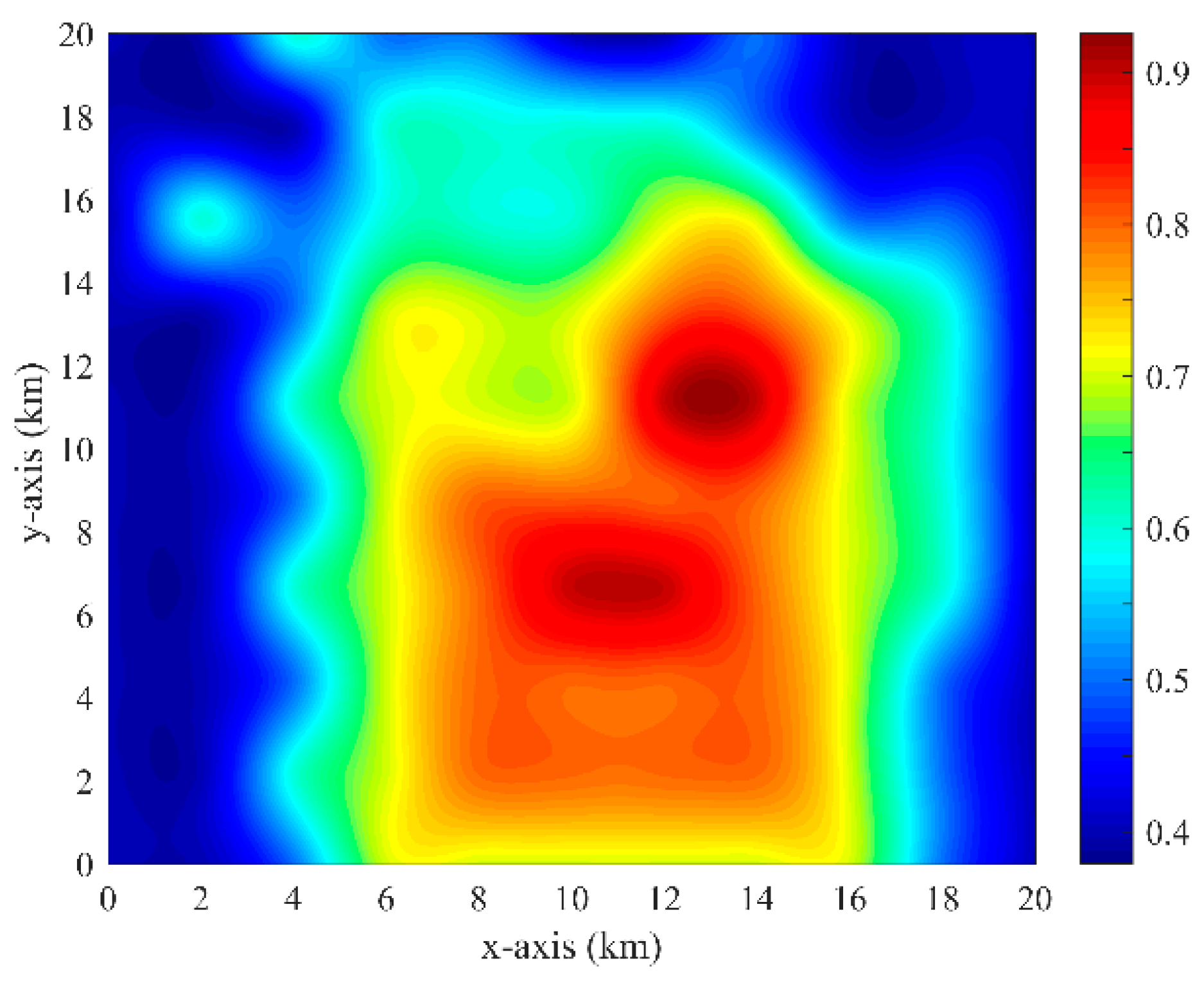
- We formulate the joint power allocation and antenna placement problem as an optimization model subject to the resource budget and area priority level. In the proposed JAPPA model, binary composite hypothesis testing is established to design the Neyman–Pearson (NP) detector for the whole surveillance area with the targets Radar Cross Section (RCS) obeying Rayleigh distribution. Compared to previous oversimplified works [19,20], the weighted NP-based logarithm likelihood ratio test (LRT) function is specified as the utility function that combines all optimization factors into a single objective function. In addition, we evaluate the average utility function values after changing the single stationary target’s position in the whole region to describe the global target detection performance of the radar network.
- We propose an efficient JAPPA strategy that incorporates antenna placement with power allocation to optimize the target detection performance in the radar network. Different from the 0–1 programming in [21,31], we choose suitable antenna deployment positions in the regional grid points to establish the non-linear mixed integer programming problem. To devise computationally feasible methods for practical applications, a two-stage local-search-based algorithm is proposed to split the coupled joint optimization. Herein, it isolates integer programming from continuous variable optimization and provides equivalent performance while requiring less computing effort.
- We develop a joint optimization closed-loop scheme for the joint antenna placement and power allocation optimization [30]. In our scheme, the optimal position results in the current cycle are used for guiding the power allocation. The detection performance will be further improved through this link, which renders a closed-loop scheme to repeat the iteration of transmitting and receiving antenna placement using the optimal power allocation scheme.
1.3. Organization
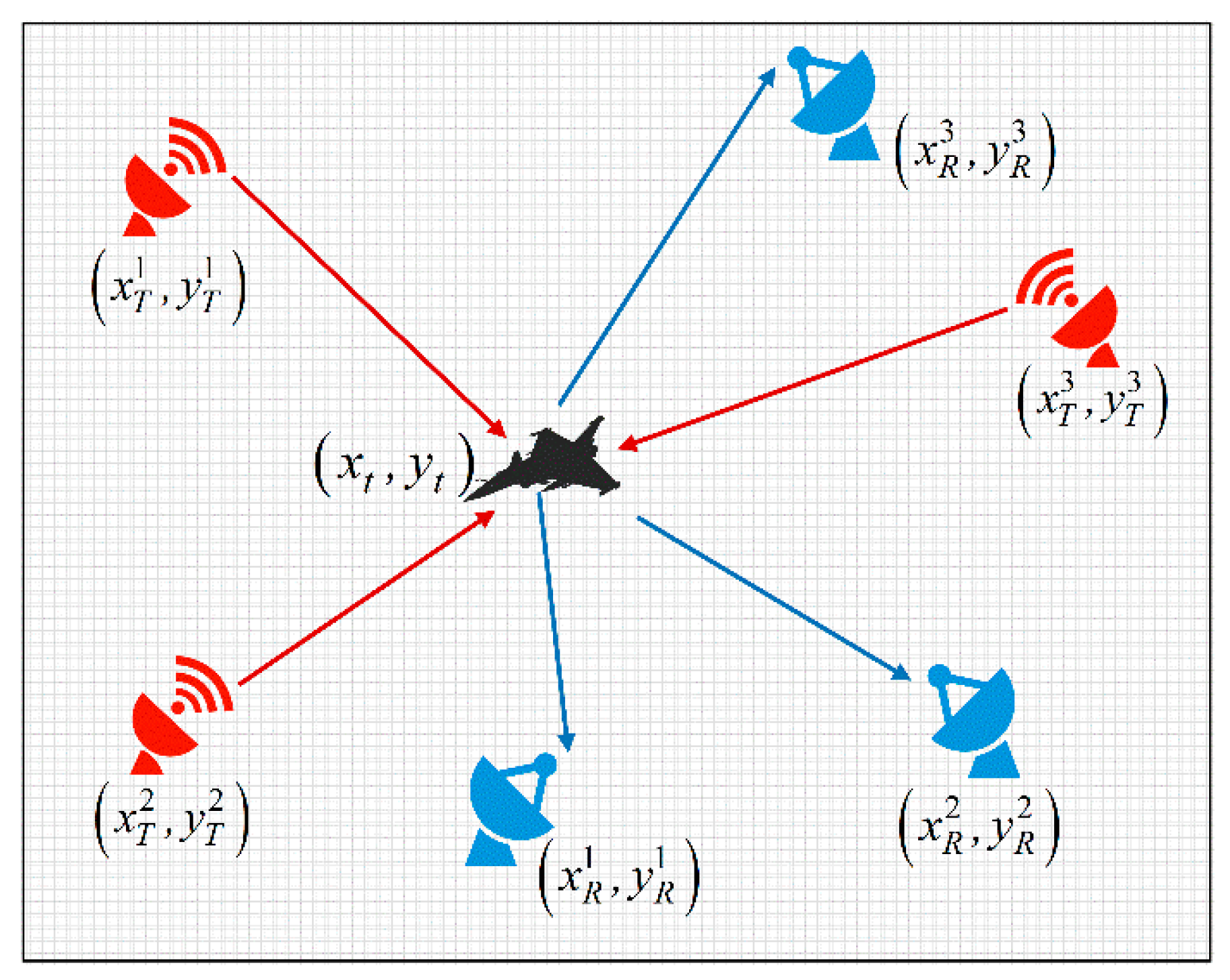
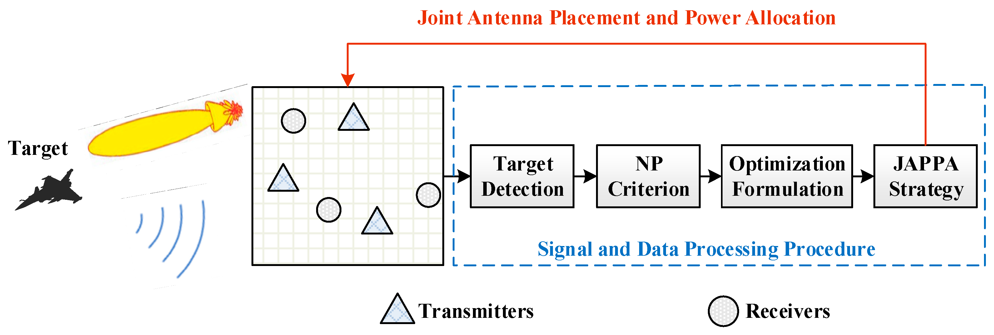
2. System Model and Detection Formulation
2.1. Signal Model
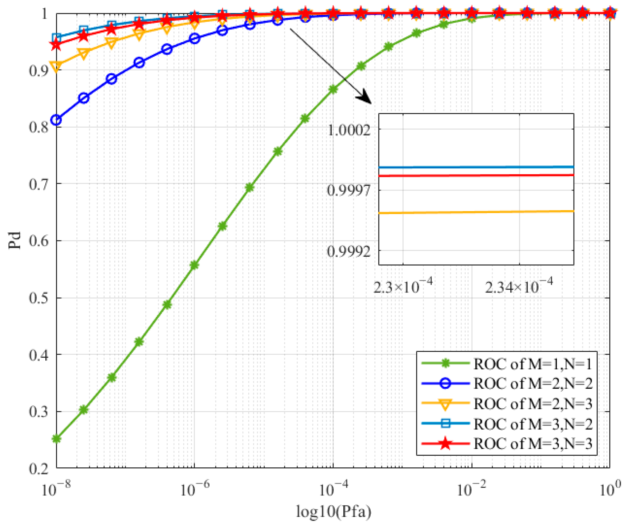
2.2. Neyman–Pearson Detection Model
3. Antenna Placement and Power Allocation Strategy
3.1. Optimization Formulation
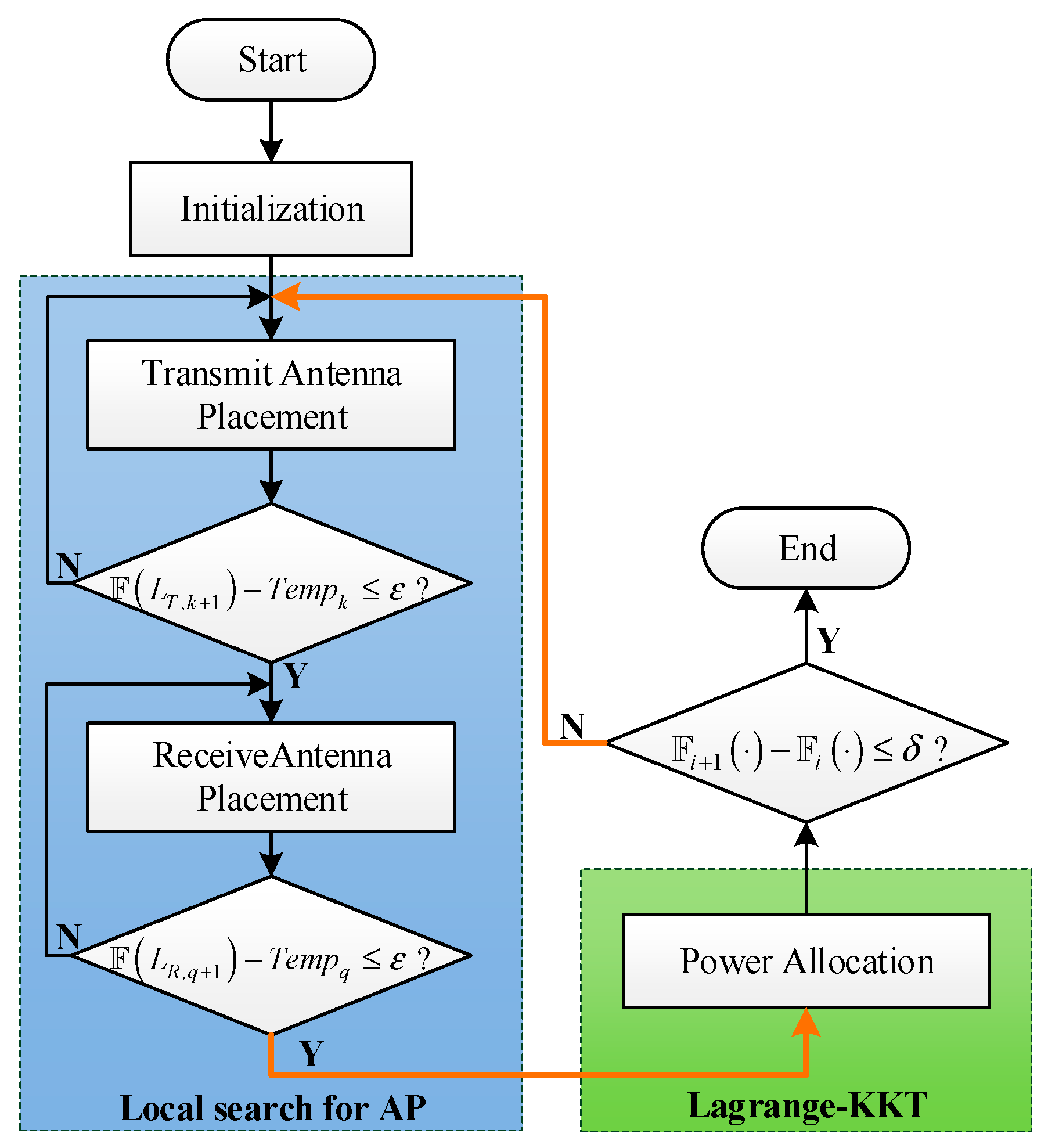
3.2. Solution Technique
3.2.1. Local Search for Antenna Placement
| Algorithm 1: Two-stage greedy dropping heuristic local search for antenna placement |
| Input: |
| Output: optimal and |
| 1 Initialize , , and ; |
| 2 double ; |
| 3 while do |
| 4 Replaces |
| 5 Recombines : substitute with a new coordinate |
| 6 if then |
| 7 |
| 8 Removes the from the set of candidate points |
| 9 end if |
| 10 |
| 11 end while |
| 12 while do |
| 13 Replaces |
| 14 Recombines : substitute with a new coordinate |
| 15 if then |
| 16 |
| 17 Removes the from the set of candidate points |
| 18 end if |
| 19 |
| 20 end while |
| 21 return , |
3.2.2. Local-Search-Based Lagrange-KKT for Power Allocation
3.3. Closed-Loop Resource Allocation Scheme
3.4. Computational Complexity Analysis
- (1)
- The local search for antenna placement;
- (2)
- The Lagrange-KKT for Power Allocation.
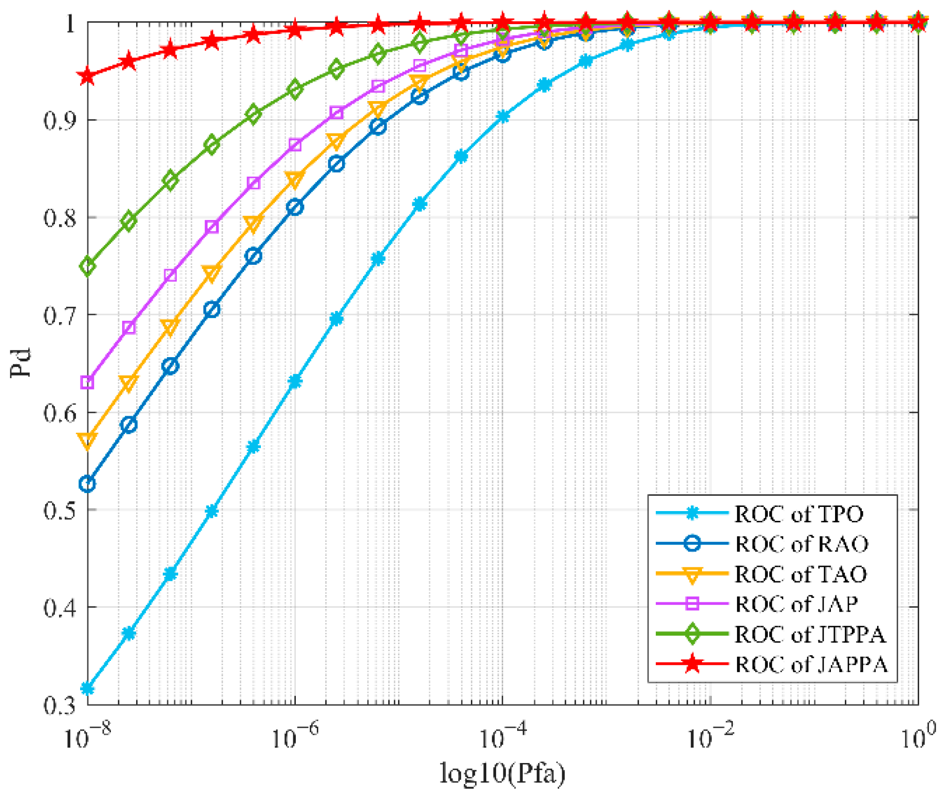
4. Simulation Results and Discussion
4.1. Factors That Affect the Results of Iterative Optimization
4.1.1. Case 1: Optimization Parameters’ Degree of Freedom
- Single-parameter optimization:
- (1)
- Transmitting antenna position optimization (TAO): The approach simply adjusts the location of the transmitting antenna to enhance the radar network’s target detection capacity.
- (2)
- Receiving antenna position optimization (RAO): The radar network transmitter sites remain constant with evenly distributed transmitting power, and only the placements of the receiving antennas are modified to improve the radar network’s detecting capability.
- (3)
- Transmit power allocation optimization (TPO): The transmitting power is efficiently allocated to increase target detection capabilities based on the random deployment of the radar network antenna space architecture.
- Two-element optimization:
- (1)
- Joint antenna placement optimization (JAP): In this experiment, the transmitting power is uniformly distributed and the antenna deployment positions are optimized using a two-stage method, in which transmitting and receiving antenna positions are iteratively optimized. The iteration completes when the increment reaches the given error limit.
- (2)
- Joint transmitter placement and power allocation optimization (JTPPA): We jointly design the transmit power allocation and transmitters’ placement to optimize radar performance criteria.
4.1.2. Case 2: Iterative Loop Containment Range
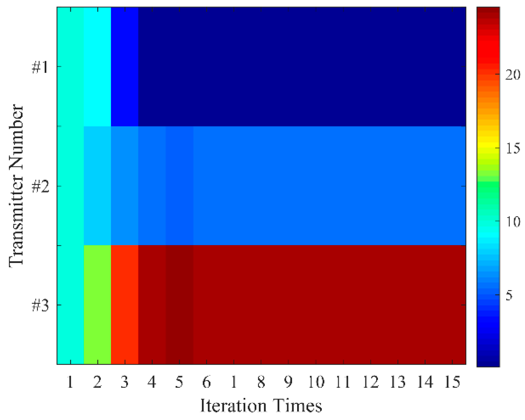
4.1.3. Case 3: Numbers of Antennas
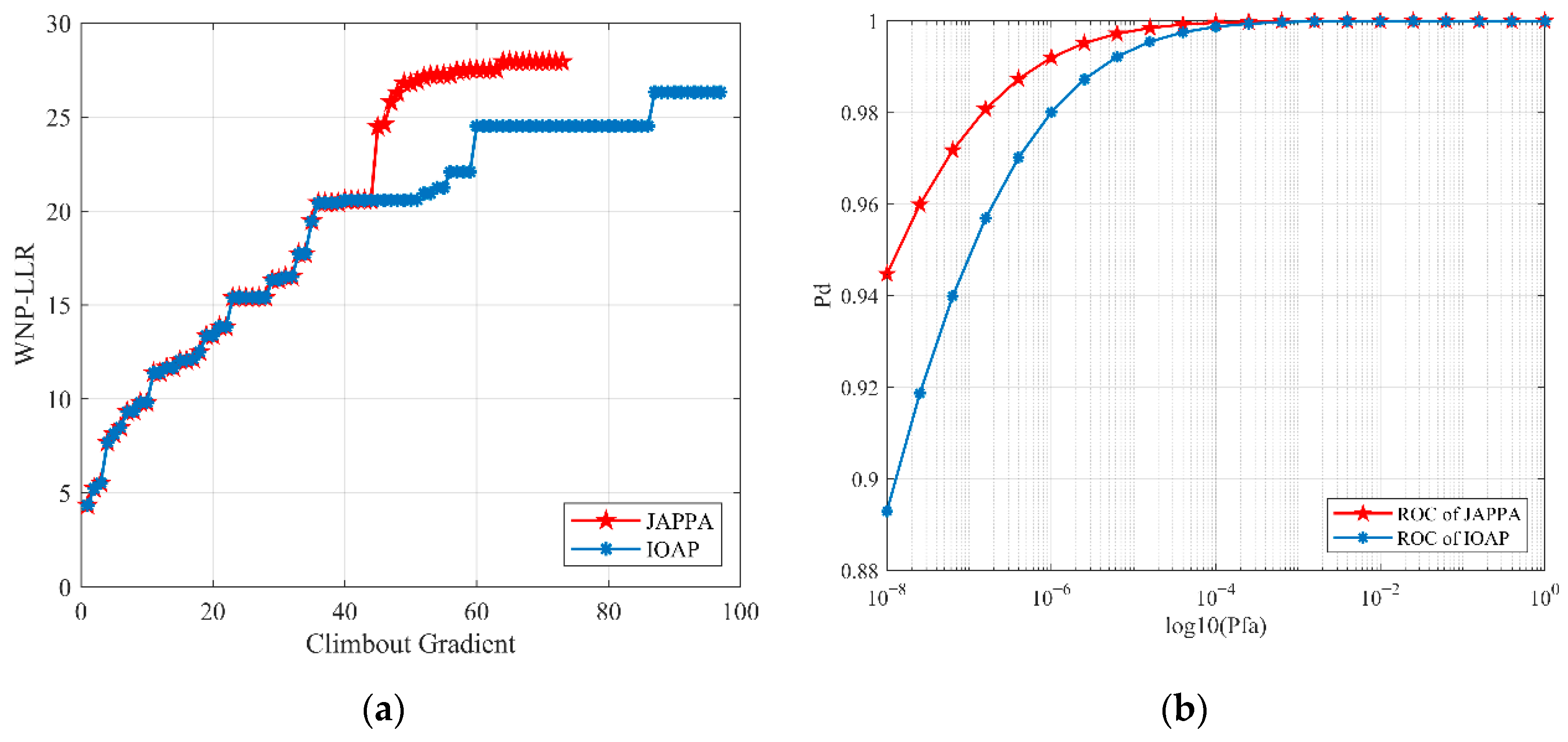
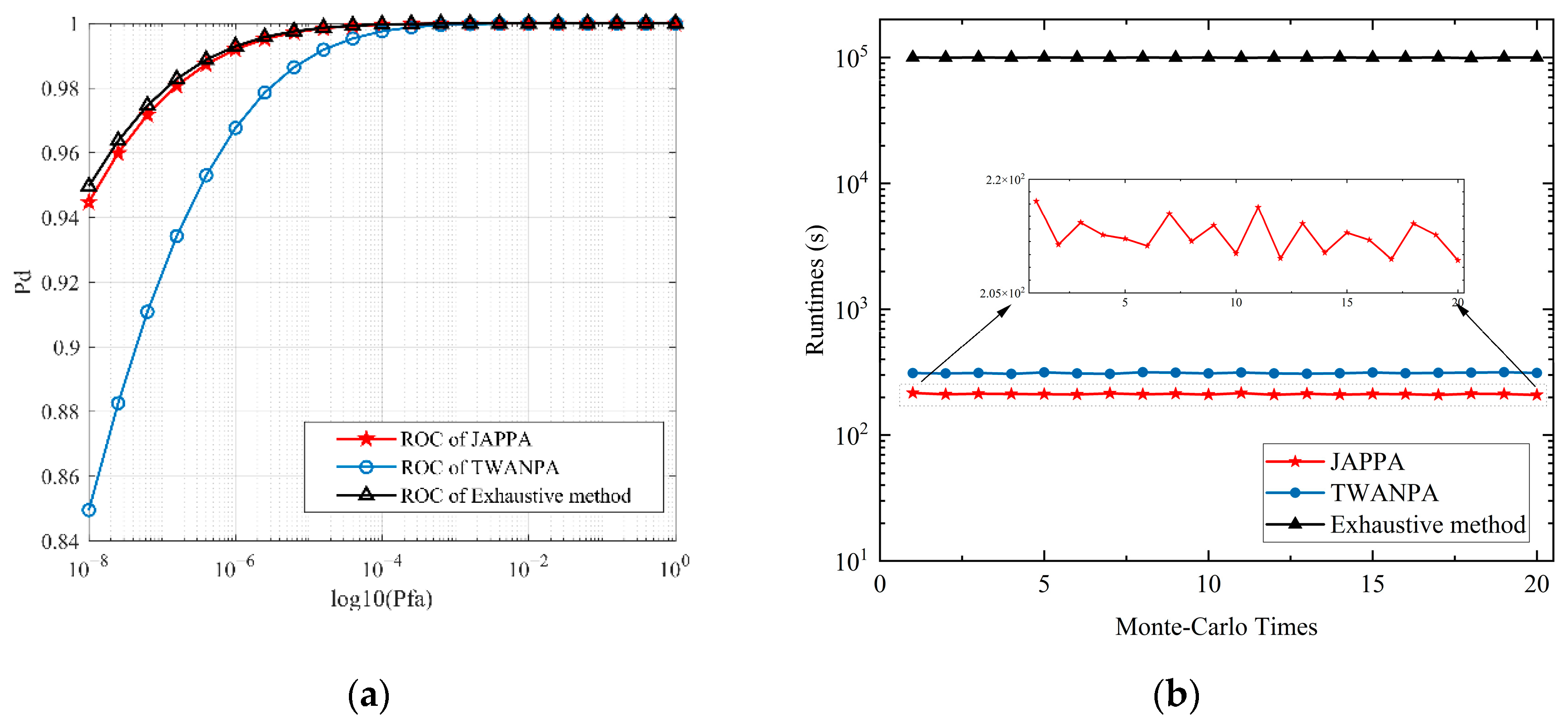
4.2. The Efficiency of the Iterative Two-Stage Closed-Loop Solver
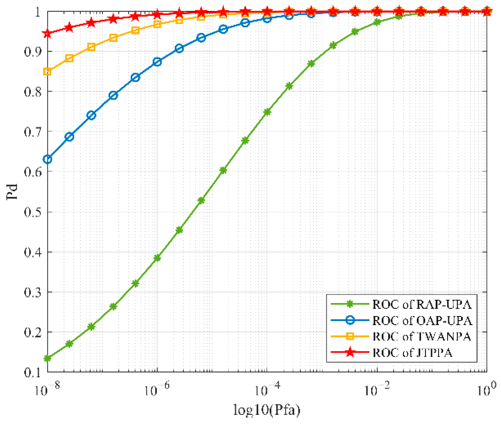
4.3. Effectiveness of the Proposed Method
- Random antenna placement with uniform power allocation (RAP-UPA): This method randomly selects the positions of the antennas with the uniform transmitting power resource allocation.
- Random antenna placement withnon-uniform power allocation (RAP-UUPA): The realistic scenario of non-uniform power allocation and random antenna placement will be considered in this simulation.
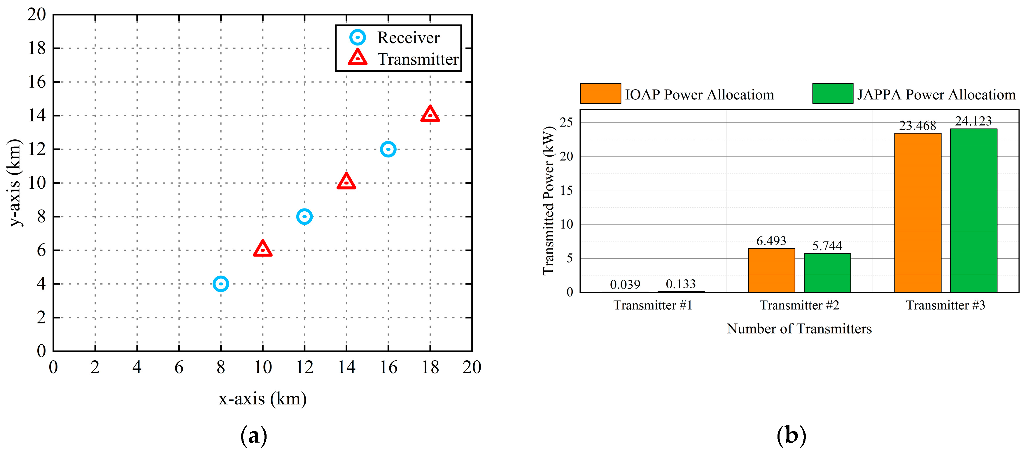
- Optimal antenna placement with uniform power allocation (OAP-UPA) [13]: In this scenario, the transmitters and receivers are optimally placed sequentially with the power consumption uniformly allocated to the transmitting antennas.
- Three-stage water-filling-type antenna placement and power allocation strategy (TWANPA) [19]: This method improves the radar detection performance through successive optimization under the total power constraint and designs a suboptimal method to effectively locate transmitting and receiving antennas under the water-filling power allocation. It completes the transmitting antenna placement using the power density criterion and positioning the receiving antenna with the SNR criterion. Subsequently, a closed-loop optimization mechanism is established by repeating the antennas’ positions using the allocated powers.
5. Conclusions
- The log-LRT function unifies the antenna position variables and transmitter power allocation variables into a single collaborative objective function, which is suitable for guiding the joint resource allocation optimization.
- The joint antenna and power allocation optimization can more effectively improve the target detection performance of the radar system.
- The proposed strategy is effective and efficient in solving the JAPPA problem.
Author Contributions
Funding
Data Availability Statement
Acknowledgments
Conflicts of Interest
Appendix A
References
- Fishler, E.; Haimovich, A.; Blum, R.; Chizhik, D.; Cimini, L.; Valenzuela, R. MIMO radar: An idea whose time has come. In Proceedings of the 2004 IEEE Radar Conference (IEEE Cat. No.04CH37509), Philadelphia, PA, USA, 29 April 2004; pp. 71–78. [Google Scholar]
- Yang, J.; Aubry, A.; Maio, A.D.; Yu, X.; Cui, G. Design of Constant Modulus Discrete Phase Radar Waveforms Subject to Multi-Spectral Constraints. IEEE Signal Process. Lett. 2020, 27, 875–879. [Google Scholar] [CrossRef]
- Yao, Y.; Liu, H.T.; Miao, P.; Wu, L.N. MIMO Radar Design for Extended Target Detection in a Spectrally Crowded Environment. IEEE Trans. Intell. Transp. Syst. 2021, 1–10. [Google Scholar] [CrossRef]
- Stoica, P. MIMO Radar Signal Processing; Wiley-IEEE Press: Hoboken, NJ, USA, 2009. [Google Scholar]
- Li, X.; Chen, H.; Zhuang, Z.; Yang, J.; Qiu, Z. Effects of transmitting correlated waveforms for co-located multi-input multi-output radar with target detection and localisation. Signal Process. IET 2013, 7, 897–910. [Google Scholar]
- Haimovich, A.M.; Blum, R.S.; Cimini, L.J. MIMO Radar with Widely Separated Antennas. IEEE Signal Process. Mag. 2008, 25, 116–129. [Google Scholar] [CrossRef]
- Gogineni, S.; Nehorai, A. Target Estimation Using Sparse Modeling for Distributed MIMO Radar. IEEE Trans. Signal Process. 2011, 59, 5315–5325. [Google Scholar] [CrossRef]
- Fishler, E.; Haimovich, A.; Blum, R.S.; Cimini, L.J.; Chizhik, D.; Valenzuela, R.A. Spatial Diversity in Radars—Models and Detection Performance. IEEE Trans. Signal Process. 2006, 54, 823–838. [Google Scholar] [CrossRef]
- He, Q.; Blum, R.S.; Haimovich, A.M. Noncoherent MIMO Radar for Location and Velocity Estimation: More Antennas Means Better Performance. IEEE Trans. Signal Process. 2010, 58, 3661–3680. [Google Scholar] [CrossRef]
- Godrich, H.; Haimovich, A.M.; Blum, R.S. Cramer Rao bound on target localization estimation in MIMO radar systems. In Proceedings of the 2008 42nd Annual Conference on Information Sciences and Systems, Princeton, NJ, USA, 19–21 March 2008; pp. 134–139. [Google Scholar]
- Gacho, J.F.A.L. Researching UAV Threat—New Challenges. In Proceedings of the 2021 International Conference on Military Technologies (ICMT), Brno, Czech Republic, 8–11 June 2021; pp. 1–6. [Google Scholar]
- Yao, Y.; Wu, L.; Liu, H.T. Robust Transceiver Design in the Presence of Eclipsing Loss for Spectrally Dense Environments. IEEE Syst. J. 2021, 15, 4334–4345. [Google Scholar] [CrossRef]
- Yi, J.; Wan, X.; Leung, H.; Lü, M. Joint Placement of Transmitters and Receivers for Distributed MIMO Radars. IEEE Trans. Aerosp. Electron. Syst. 2017, 53, 122–134. [Google Scholar] [CrossRef]
- Chitgarha, M.M.; Radmard, M.; Majd, M.N.; Nayebi, M.M. Improving MIMO radar’s performance through receivers’ positioning. IET Signal Process. 2017, 11, 622–630. [Google Scholar] [CrossRef]
- Wang, Y.; Yang, S.; Zhou, T.; Li, N. Geometric Optimization of Distributed MIMO Radar Systems with Spatial Distance Constraints. IEEE Access 2020, 8, 199227–199241. [Google Scholar] [CrossRef]
- Feng, H.Z.; Liu, H.W.; Yan, J.K.; Dai, F.Z.; Fang, M. A fast efficient power allocation algorithm for target localization in cognitive distributed multiple radar systems. Signal Process. 2016, 127, 100–116. [Google Scholar] [CrossRef]
- Yan, J.; Pu, W.; Liu, H.; Jiu, B.; Bao, Z. Robust Chance Constrained Power Allocation Scheme for Multiple Target Localization in Colocated MIMO Radar System. IEEE Trans. Signal Process. 2018, 66, 3946–3957. [Google Scholar] [CrossRef]
- Shi, C.G.; Wang, Y.J.; Wang, F.; Salous, S.; Zhou, J.J. Power resource allocation scheme for distributed MIMO dual-function radar-communication system based on low probability of intercept. Digit. Signal Prog. 2020, 106, 12. [Google Scholar] [CrossRef]
- Radmard, M.; Chitgarha, M.M.; Majd, M.N.; Nayebi, M.M. Antenna placement and power allocation optimization in MIMO detection. IEEE Trans. Aerosp. Electron. Syst. 2014, 50, 1468–1478. [Google Scholar] [CrossRef]
- Jebali, S.; Keshavarz, H.; Allahdadi, M. Joint Power allocation and target detection in distributed MIMO radars. IET Radar Sonar Navig. 2021, 15, 1433–1447. [Google Scholar] [CrossRef]
- Ma, B.; Chen, H.; Sun, B.; Xiao, H. A Joint Scheme of Antenna Selection and Power Allocation for Localization in MIMO Radar Sensor Networks. IEEE Commun. Lett. 2014, 18, 2225–2228. [Google Scholar] [CrossRef]
- Xie, M.C.; Yi, W.; Kirubarajan, T.; Kong, L.J. Joint Node Selection and Power Allocation Strategy for Multitarget Tracking in Decentralized Radar Networks. IEEE Trans. Signal Process. 2018, 66, 729–743. [Google Scholar] [CrossRef]
- Godrich, H.; Petropulu, A.P.; Poor, H.V. Sensor Selection in Distributed Multiple-Radar Architectures for Localization: A Knapsack Problem Formulation. IEEE Trans. Signal Process. 2012, 60, 247–260. [Google Scholar] [CrossRef]
- Berenguer, I.; Xiaodong, W.; Krishnamurthy, V. Adaptive MIMO antenna selection via discrete stochastic optimization. IEEE Trans. Signal Process. 2005, 53, 4315–4329. [Google Scholar] [CrossRef] [Green Version]
- He, Q.; Blum, R.S.; Haimovich, A.M.; He, Z. Antenna placement for velocity estimation using MIMO radar. In Proceedings of the 2008 42nd Asilomar Conference on Signals, Systems and Computers, Pacific Grove, CA, USA, 26–29 October 2008; pp. 619–623. [Google Scholar]
- Ajorloo, A.; Amini, A.; Tohidi, E.; Bastani, M.H.; Leus, G. Antenna Placement in a Compressive Sensing-Based Colocated MIMO Radar. IEEE Trans. Aerosp. Electron. Syst. 2020, 56, 4606–4614. [Google Scholar] [CrossRef]
- Yuan, Y.; Yi, W.; Hoseinnezhad, R.; Varshney, P.K. Robust Power Allocation for Resource-Aware Multi-Target Tracking with Colocated MIMO Radars. IEEE Trans. Signal Process. 2021, 69, 443–458. [Google Scholar] [CrossRef]
- Chavali, P.; Nehorai, A. Scheduling and Power Allocation in a Cognitive Radar Network for Multiple-Target Tracking. IEEE Trans. Signal Process. 2012, 60, 715–729. [Google Scholar] [CrossRef]
- Zhang, H.W.; Liu, W.J.; Xie, J.W.; Zhang, Z.J.; Lu, W.L. Joint Subarray Selection and Power Allocation for Cognitive Target Tracking in Large-Scale MIMO Radar Networks. IEEE Syst. J. 2020, 14, 2569–2580. [Google Scholar] [CrossRef]
- Shia, C.; Ding, L.; Wang, F.; Zhou, J.; Yan, J. Collaborative radar node selection and transmitter resource allocation algorithm for target tracking applications in multiple radar architectures. Digit. Signal Prog. 2022, 121, 103318. [Google Scholar] [CrossRef]
- Zhang, H.; Xie, J.; Shi, J.; Zhang, Z.; Fu, X. Sensor Scheduling and Resource Allocation in Distributed MIMO Radar for Joint Target Tracking and Detection. IEEE Access 2019, 7, 62387–62400. [Google Scholar] [CrossRef]
- Skolnik, M.I. Radar Handbook; McGraw-Hill Education: New York, NY, USA, 1990. [Google Scholar]
- News, S.; News, S. Detection, Estimation and Modulation Theory; John Wiley & Sons, Inc.: Hoboken, NJ, USA, 1968. [Google Scholar]
- Yuan, Y.; Yi, W.; Kirubarajan, T.; Kong, L.J. Scaled accuracy based power allocation for multi-target tracking with colocated MIMO radars. Signal Process. 2019, 158, 227–240. [Google Scholar] [CrossRef]
- Yan, J.K.; Liu, H.W.; Jiu, B.; Chen, B.; Liu, Z.; Bao, Z. Simultaneous Multibeam Resource Allocation Scheme for Multiple Target Tracking. IEEE Trans. Signal Process. 2015, 63, 3110–3122. [Google Scholar] [CrossRef]
- Boyd, S.; Vandenberghe, L. Convex Optimization; Cambridge University Press: Cambridge, UK, 2004. [Google Scholar]
- Boyd, S.; Vandenberghe, L.; Faybusovich, L. Convex Optimization. IEEE Trans. Autom. Control. 2006, 51, 1859. [Google Scholar]
- Bertsekas, D.P.; Nedic, A.; Ozdaglar, A.E. Convex Analysis and Optimization; Pitman Advanced Pub. Program; MIT: Cambridge, MA, USA, 2003. [Google Scholar]
- Stoica, P.; Selen, Y. Cyclic minimizers, majorization techniques, and the expectation-maximization algorithm: A refresher. IEEE Signal Process. Mag. 2004, 21, 112–114. [Google Scholar] [CrossRef]
- Mahafza, B.R.; Elsherbeni, A. MATLAB Simulations for Radar Systems Design; Chapman and Hall/CRC: London, UK, 2003. [Google Scholar]
- Liang, J.; Zhang, T.; Yang, Y.; Cui, G.; Yang, J. An efficient antenna placement method for MIMO radar under the situation of multiple interference regions. In Proceedings of the 2017 20th International Conference on Information Fusion (Fusion), Xi’an, China, 10–13 July 2017. [Google Scholar]
- Zhang, H.; Liu, W.; Zhang, Z.; Lu, W.; Xie, J. Joint Target Assignment and Power Allocation in Multiple Distributed MIMO Radar Networks. IEEE Syst. J. 2020, 15, 694–704. [Google Scholar] [CrossRef]
- Ristic, B.; Rosenberg, L.; Du, Y.K.; Wang, X.; Williams, J. A Bernoulli track-before-detect filter for maritime radar. IET Radar Sonar Navig. 2019, 14, 356–363. [Google Scholar] [CrossRef]
- Zhang, H.; Liu, W.; Shi, J.; Fei, T.; Zong, B. Joint detection threshold optimization and illumination time allocation strategy for cognitive tracking in a networked radar system. IEEE Trans. Signal Process. 2022; to be published. [Google Scholar]
- He, B.; Su, H.; Huang, J. Joint Beamforming and Power Allocation Between A Multistatic MIMO Radar Network and Multiple Targets Using Game Theoretic Analysis. Digit. Signal Prog. 2021, 115, 103085. [Google Scholar] [CrossRef]


| Algorithm | Exhaustive Search | TWANPA Method | JAPPA Strategy |
|---|---|---|---|
| Computational complexity |
| Names | Symbols | Settings |
|---|---|---|
| Transmitting Antenna Gain | 30 dB | |
| Receiving Antenna Gain | 30 dB | |
| Processing Gain At Receiver | 20 dB | |
| Carrier Frequency | 10 GHz | |
| Target Average RCS | 2 m2 | |
| Radar Network Scattering Loss | 0 dB | |
| Radar Network Receiving Loss | 0 dB | |
| Noise Factor | 4 dB | |
| Bandwidth | 5 MHz | |
| Transmit Power | 30 KW | |
| Minimum Transmit Power | 0 KW | |
| Maximum Transmit Power | 30 KW |
| Transmitter | x (km) | y (km) |
|---|---|---|
| #1 | 14 | 10 |
| #2 | 2 | 14 |
| #3 | 4 | 18 |
| Transmitter | x (km) | y (km) |
|---|---|---|
| #1 | 4 | 2 |
| #2 | 10 | 6 |
| #3 | 14 | 10 |
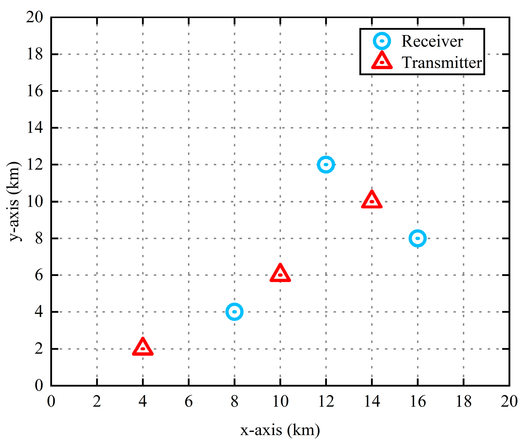
| Transmitter | x (km) | y (km) |
|---|---|---|
| #1 | 16 | 8 |
| #2 | 12 | 12 |
| #3 | 8 | 4 |
| Transmitter | #1 | #2 | #3 |
|---|---|---|---|
| Power Allocation (KW) | 0.133 | 5.744 | 24.123 |
| Transmitter | x (km) | y (km) |
|---|---|---|
| #1 | 18 | 14 |
| #2 | 10 | 6 |
| #3 | 14 | 10 |
| Transmitter | x (km) | y (km) |
|---|---|---|
| #1 | 16 | 12 |
| #2 | 12 | 8 |
| #3 | 8 | 4 |
Publisher’s Note: MDPI stays neutral with regard to jurisdictional claims in published maps and institutional affiliations. |
© 2022 by the authors. Licensee MDPI, Basel, Switzerland. This article is an open access article distributed under the terms and conditions of the Creative Commons Attribution (CC BY) license (https://creativecommons.org/licenses/by/4.0/).
Share and Cite
Qi, C.; Xie, J.; Zhang, H. Joint Antenna Placement and Power Allocation for Target Detection in a Distributed MIMO Radar Network. Remote Sens. 2022, 14, 2650. https://doi.org/10.3390/rs14112650
Qi C, Xie J, Zhang H. Joint Antenna Placement and Power Allocation for Target Detection in a Distributed MIMO Radar Network. Remote Sensing. 2022; 14(11):2650. https://doi.org/10.3390/rs14112650
Chicago/Turabian StyleQi, Cheng, Junwei Xie, and Haowei Zhang. 2022. "Joint Antenna Placement and Power Allocation for Target Detection in a Distributed MIMO Radar Network" Remote Sensing 14, no. 11: 2650. https://doi.org/10.3390/rs14112650
APA StyleQi, C., Xie, J., & Zhang, H. (2022). Joint Antenna Placement and Power Allocation for Target Detection in a Distributed MIMO Radar Network. Remote Sensing, 14(11), 2650. https://doi.org/10.3390/rs14112650