Article

An Open Data Approach for Estimating Vegetation Gross Primary Production at Fine Spatial Resolution

1
School of Atmospheric Sciences, Southern Marine Science and Engineering Guangdong Laboratory (Zhuhai), Sun Yat-sen University, Zhuhai 519082, China
2
International Research Center of Big Data for Sustainable Development Goals, Beijing 100094, China
*
Author to whom correspondence should be addressed.
Remote Sens. 2022, 14(11), 2651; https://doi.org/10.3390/rs14112651
Submission received: 28 April 2022 / Revised: 25 May 2022 / Accepted: 30 May 2022 / Published: 1 June 2022
(This article belongs to the Section Biogeosciences Remote Sensing)

Abstract

:
Accurate simulations of the spatial and temporal changes in vegetation gross primary production (GPP) play an important role in ecological studies. Previous studies highlighted large uncertainties in GPP datasets based on satellite data with coarse spatial resolutions (>500 m), and implied the need to produce high-spatial-resolution datasets. However, estimating fine spatial resolution GPP is time-consuming and requires an enormous amount of computing storage space. In this study, based on the Eddy Covariance-Light Use Efficiency (EC-LUE) model, we used Google Earth Engine (GEE) to develop a web application (EC-LUE APP) to generate 30-m-spatial-resolution GPP estimates within a region of interest. We examined the accuracy of the GPP estimates produced by the APP and compared them with observed GPP at 193 global eddy covariance sites. The results showed the good performance of the EC-LUE APP in reproducing the spatial and temporal variations in the GPP. The fine-spatial-resolution GPP product (GPPL) explained 64% of the GPP variations and had fewer uncertainties (root mean square error = 2.34 g C m−2 d−1) and bias (−0.09 g C m−2 d−1) than the coarse-spatial-resolution GPP products. In particular, the GPPL significantly improved the GPP estimations for cropland and dryland ecosystems. With this APP, users can easily obtain 30-m-spatial-resolution GPP at any given location and for any given year since 1984.

Graphical Abstract

1. Introduction

Vegetation gross primary production (GPP), as the principal component of terrestrial ecosystems, plays an important role in supporting global sustenance and energy cycles, regulating the carbon balance and alleviating the rise in atmospheric CO2 concentrations and global climate change. However, the modeling of GPP is one of the largest sources of uncertainty in global carbon cycle [1,2]. The current satellite-derived GPP products are based on coarse-spatial-resolution data (500 m~8 km), which cannot reproduce the spatial heterogeneity of GPP and leads to uncertainties in GPP estimates [3]. Previous studies showed that the spatial heterogeneity in farmland led to a 30% underestimation in GPP from the agroecosystem [4], while Chen et al. (2010) showed a 5% overestimation in forest ecosystems [5]. Therefore, the improved capturing of the spatial heterogeneity of landscapes can reduce GPP simulation uncertainty.
With fine-spatial-resolution remote sensing data as the input, light use efficiency (LUE)-based GPP models, which account for both physiological process and vegetation structure change, can precisely characterize the GPP in heterogeneous regions [6,7]. Studies showed that the GPP derived from fine-spatial-resolution satellite-based datasets has a better performance than coarse-resolution GPP products because fine-resolution satellite data can capture the heterogeneity of vegetation cover [6]. For example, a LUE model driven by fine-spatial-resolution remote sensing data can reduce GPP simulation uncertainties by 20% [4]. Gitelson et al. (2012) showed that fine-spatial-resolution GPP driven by a LUE model captured the spatial and temporal changes in GPP in a typical agroecosystem [8]. Past researches focused on how fine-spatial-resolution data improved GPP estimation [9,10], but the lack of multi-site studies prevented the assessment of how spatial heterogeneity influenced GPP modeling globally.
More importantly, the collection of fine-scale remotely sensed data requires a significant amount of storage space, and computing fine-spatial-resolution GPP is time-consuming. For example, the Landsat 8 project acquired around 500,000 images at a 30-meter spatial resolution per year, requiring an enormous data storage capacity (~600 TB) [11]. Before users can execute a study, a large amount of time is spent accessing the data and completing the necessary preprocessing steps. Thus, it is difficult to download such a significant amount of data to derive fine-spatial-resolution GPP for various sites. Using the Google Earth Engine (GEE) platform to generate such fine-spatial-resolution GPP products on demand can save significant time and data storage. Furthermore, the revisit periods of fine-spatial-resolution-satellite remote sensing data (for example, ~16 days for Landsat, ~5 days for Sentinel-2), are much longer than those of coarse spatial resolution, which can provide almost two observations each day in the case of moderate-resolution-imaging spectro-radiometer (MODIS) and advanced very-high-resolution radiometer (AVHRR) series. Therefore, the availability of fine spatial remote sensing data may fail to represent the growing condition of vegetation and lead to high uncertainties in GPP modeling. However, few studies have focused on this topic.
In this study, we used the Eddy Covariance-Light Use Efficiency (EC-LUE) model [12] and long-time-series Landsat data as the input to derive fine-spatial-resolution GPP and compared it to the GPP driven by coarse-spatial-resolution remote sensing data. We asked the following questions: (1) How and where did the fine-spatial-resolution remote sensing data improve the GPP estimation compared to coarse-spatial-resolution GPP? (2) How did the data missing from Landsat affect GPP modeling accuracy? To address these questions, we built a web application (APP) on GEE to generate GPP with Landsat 30-meter-spatial-resolution data and compared the fine spatial resolution GPP with the existing coarse-spatial-resolution GPP products. With this APP, researchers can easily obtain fine-spatial-resolution GPP for their purposes and use it for further research.

2. Materials and Data

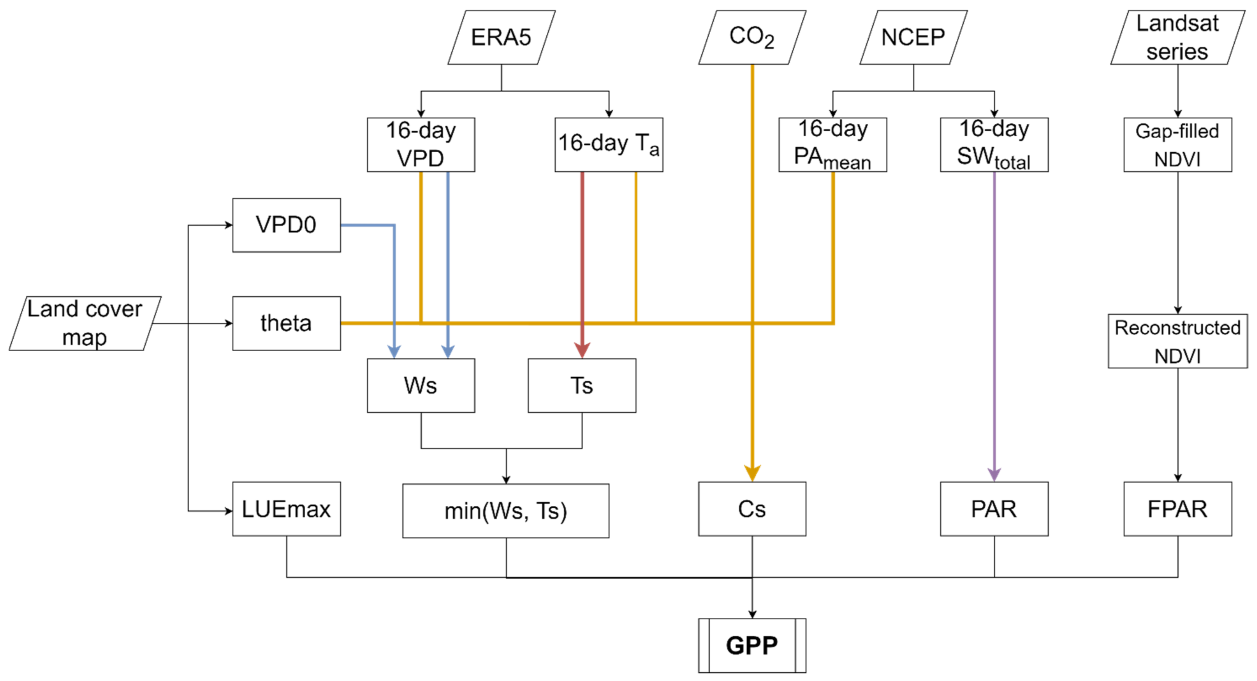
2.1. Revised EC-LUE Model

The EC-LUE model framework has the following form [12]:
GPP = FPAR × PAR × ε max × C s × min T s , W s
where FPAR is the fraction of absorbed photosynthetically active radiation calculated by fine-spatial-resolution normalized difference vegetation index (NDVI), calculated as:
FPAR = 1.24 × NDVI + 0.168
The NDVI in Equation (2) is calculated from red and near-infrared band reflectance from different-spatial-resolution remote sensing data (e.g., Landsat, MODIS, AVHRR). The PAR in Equation (1) is the photosynthetically active radiation (MJ m−2); εmax (LUEmax, g C MJ−1) is the maximal light use efficiency, which is biome-specific; Cs, Ts, and Ws represent the downward-regulation scalars for the respective effects of atmospheric CO2 concentration (ppm), temperature (°C), and atmospheric water demand (vapor pressure deficit, VPD, in kPa) on LUE, respectively; min denotes the minimum value of Ts and Ws. The Ts is calculated as:
Ts = Ta Tmin × Ta Tmax Ta Tmin × Ta Tmax Ta Topt 2
where Ta is the air temperature. The Tmin, Tmax, and Topt are set as 0, 40, and 20.33 °C in the model, respectively. The Ws is calculated as:
Ws = VPD 0 VPD 0 + VPD
where VPD0 is biome-specific half-saturation coefficient of the VPD (in k Pa). The Cs is calculated as:
Cs = Ci ϑ Ci + 2 ϑ
with Ci as leaf internal CO2 concentration [12]. The ϑ in Equation (5) is the CO2 compensation point in the absence of dark respiration, which is also biome-specific [3]. Since the NDVI data sources are different from those used by Yuan et al. (2019) [12], we needed to optimize the model coefficients based on the time series of continuous Landsat NDVI. The fine-spatial-resolution GPP model framework is shown in Figure 1.
To evaluate the merit of fine-spatial-resolution GPP based on reconstructed Landsat data (GPPL), we compared GPPL with the GPP measured at FLUXNET towers (GPPFLUX). Next, we compared GPPL with two other coarse-spatial-resolution GPP products based on the revised EC-LUE model with MODIS and AVHRR data as input, named GPPM and GPPA [3], respectively. The GPPM is driven by MODIS-based 500-m LAI product [13]. The GPPA is based on AVHRR data at 0.05 degrees (~8km) of spatial resolution.

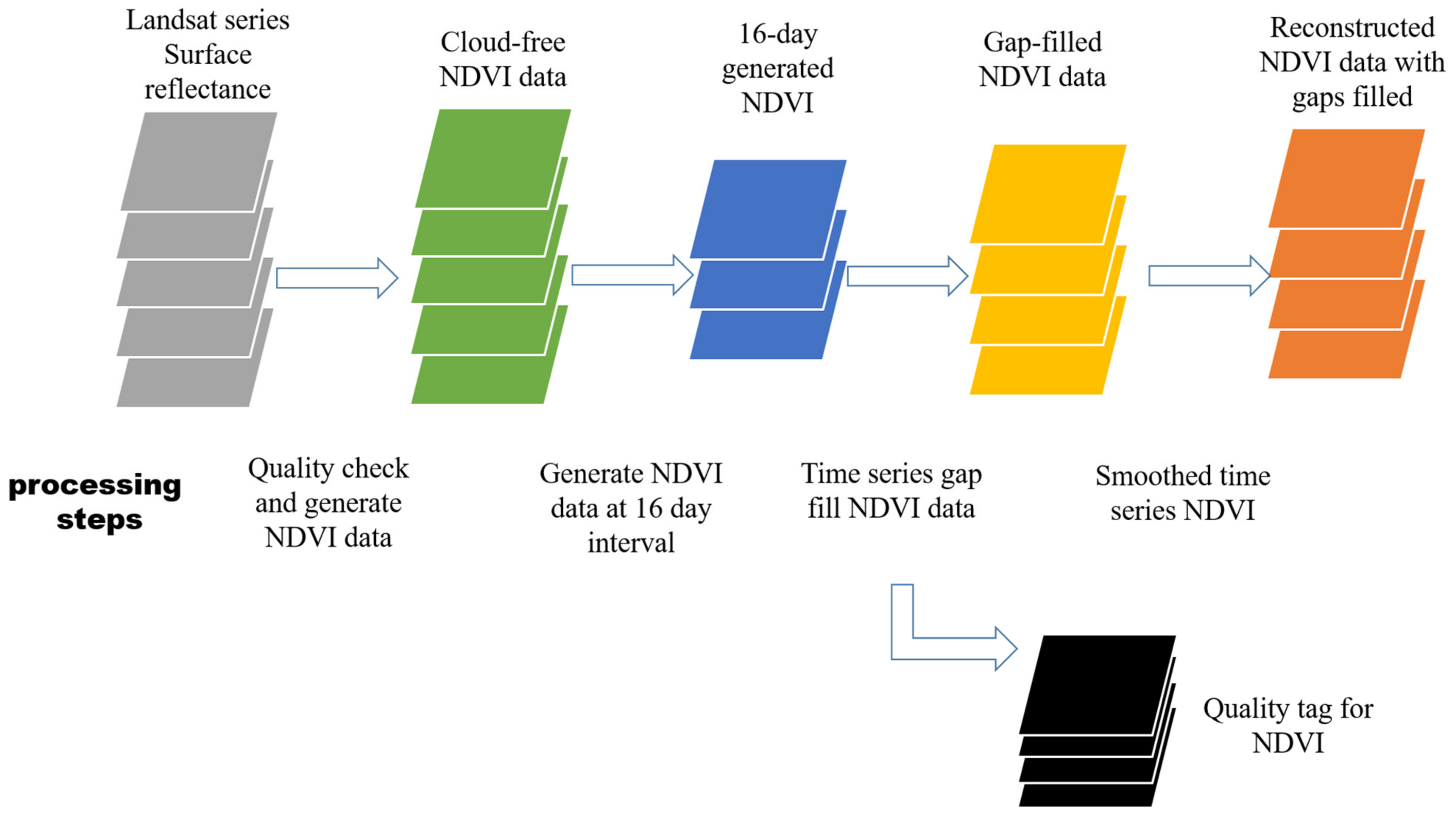
2.2. Reconstructed Landsat 30-m NDVI Data

Around 35% of fine-spatial-resolution Landsat data are missing because of cloud cover and long revisit periods [14]. Before we optimized the model coefficients, we used the following steps to reconstruct spatially and temporally continuous Landsat NDVI data (Figure 2).
We chose the surface reflectance data of Landsat Collection 2 Tier 1. We set a data selection rule to minimize the scan line corrector (SLC)-off effect in Landsat 7 Enhanced Thematic Mapper Plus (ETM+): (i) from 1984 to 2002, we selected all the available Landsat data from Landsat 5 and Landsat 7; (ii) from 2003 to 2011, we only used data from Landsat 5; from 2011 to 2013, we chose Landsat 7 data; (iii) after 2013, we only used Landsat 8 data.
  • We extracted the cloud-free pixels by using the cloud mask in the Landsat surface reflectance product.
  • We used the cloud-free pixels’ reflectance to derive the NDVI. Before we calculated the NDVI, we inter-calibrated the red and near-infrared reflectance in Landsat 5 Thematic Mapper (TM), Landsat 7 ETM+, and Landsat 8 Operational Land Imager (OLI). The TM and ETM+ have similar band settings and research has shown that their NDVIs are consistent [15]. However, the reflective wavelength differences between ETM+ and OLI still affected the NDVI values [16]. Therefore, we used the coefficients in [16] to normalize the red and near-infrared band reflectance in OLI and ETM+. Next, we derived the NDVI from all the inter-calibrated cloud-free surface reflectance. After calculating the NDVI for each image, we generated the NDVI at each 16-day interval and set the highest NDVI at each pixel during this period as the 16-day interval NDVI.
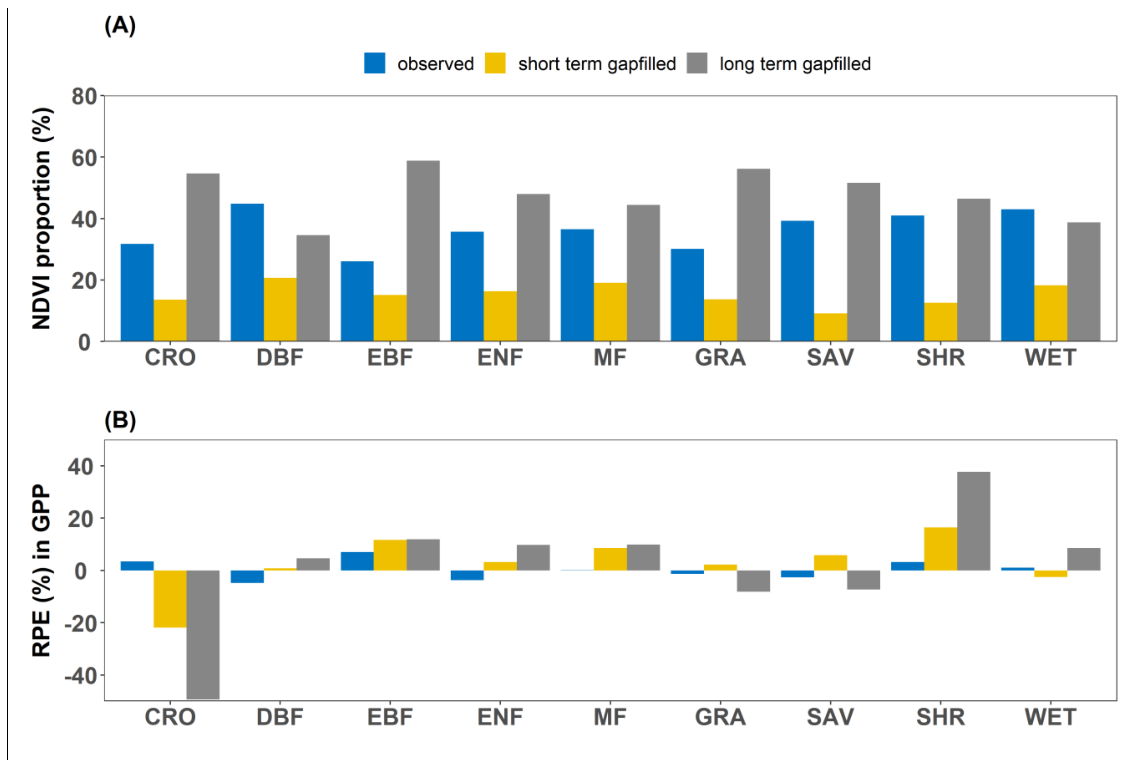
  • We performed NDVI gap-filling and wrote the quality control tag (QCtag) in the data quality layer. For pixels with NDVI observation, we wrote QCtag as 0 and kept the NDVI data. When the 16-day NDVI value was missing, we filled it by the linear interpolation method of two NDVI values of nearby dates. If the two nearby NDVI values were observed within 48 days, we defined this gap-filled NDVI as short-term gap-filled NDVI, and the QCtag was set as 1, which indicated that the reconstructed NDVI was based on short-term gap-filled data. If the two nearby NDVI values were more than 48 days apart, we defined this gap-filled NDVI as a long-term gap-filled NDVI, and the QCtag was set to 2 to indicate that the reconstructed NDVI was based on long-term gap-filled data. The data description of the gap-filled and reconstructed NDVI is shown in Table 1.
  • We used the Savitzky–Golay filter with a window size = 3, an adaptation strength = 5 to smooth the NDVI data in the time series of each pixel. We were able to derive the time-series-reconstructed 30-meter-spatial-resolution NDVI of any given study area.

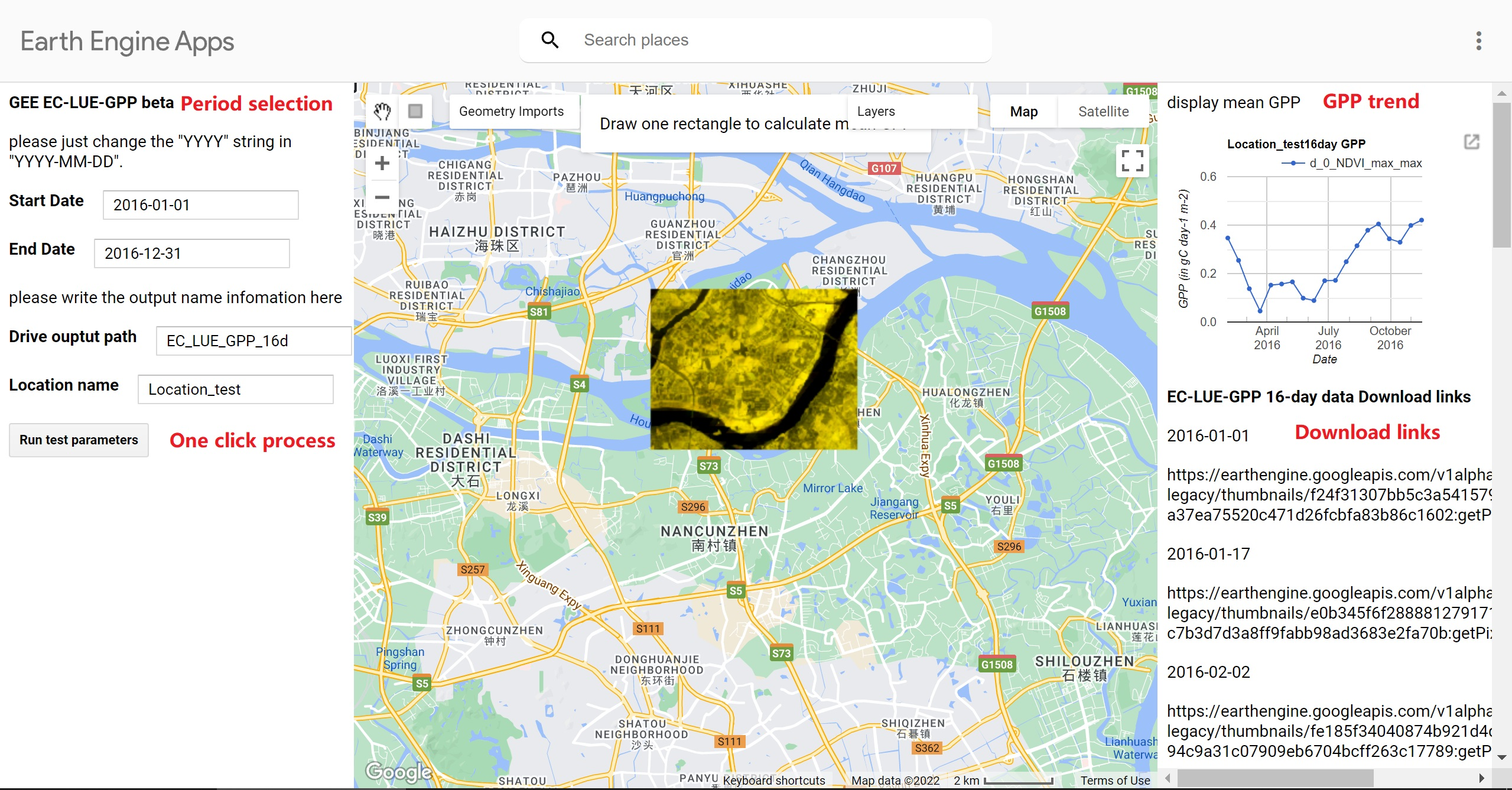
2.3. Generating GPP on GEE

We generated the 30-meter-spatial-resolution GPP at 16-day intervals on the GEE platform. The GEE is an open-access platform and provides access to Landsat 5, 7, and 8 data from 1984 to the present. Before we generated the GPP, we needed to prepare the time-series-reconstructed NDVI data, climatic data, and vegetation classification data. We summarized the climatic data at each 16-day interval. The PAR was transferred to the GEE platform from the short-wave radiation (SW) dataset from the National Centers for Environmental Prediction (NCEP) Climate Forecast System (CFS), calculated as:
PAR = SW 6 h × 0.45 × 6 × 3600 1000000 × 16
where the original SW6h is in W m−2. After transferring the PAR from equation (3), it was changed to MJ m−2 day−1. Air temperature and VPD were derived from the ERA5 dataset (https://www.ecmwf.int/en/forecasts/datasets/reanalysis-datasets/era5, accessed on 20 April 2022). The VPD was calculated from 2-m daily mean dewpoint temperature and 2-m air temperature at each 16-day interval [12]. We used a similar method to obtain a 16-day mean surface pressure. The CO2 concentration at each 16-day interval was averaged from the nearest month’s CO2 data in the dataset of Trends in Atmospheric Carbon Dioxide (https://gml.noaa.gov/ccgg/trends/data.html, accessed on 31 December 2021). We used the dynamic land-cover classification map (GLC-FCS30, Zhang et al., 2021 [17], https://data.casearth.cn/thematic/glc_fcs30?lang=en_US, accessed on 15 May 2022), which changed every five years from 1980 to 2020, with a fine classification system at 30-meter spatial resolution to classify the vegetation. The data sources are shown in Table 2.
Next, we optimized the model coefficients for the fine-spatial-resolution revised EC-LUE model. We used the reconstructed fine-resolution NDVI from Section 2.2, 16-day interval climatic data and the FLUXNET sites’ 16-day mean GPP from 2000 to 2014 [18] to optimize the model coefficients with the Markov Chain Monte Carlo approach in Huang et al. (2021) [19]. We quantified the GPP data quality by quality tag (NEE_VUT_MEAN_QC) in FLUXNET2015 dataset. When the 16-day mean NEE_VUT_MEAN_QC was less than 0.75, we defined the GPP at this 16-day point as gap-filled GPP; we defined the others as observed GPP. In the step of optimizing the model coefficients, we generated the GPP at 16-day intervals from 95 selected sites, in a similar way to Zheng et al. (2020) [3]. Next, in each site, we chose the odd years as the calibration dataset and the remaining half as the validation dataset. We optimized the coefficients with all the data in the calibration dataset at all the sites from nine vegetation types, including deciduous broadleaf forest (DBF), evergreen broadleaf forest (EBF), evergreen needleleaf forest (ENF), mixed forest (MF), grassland (GRA), savanna (SAV), shrubland (SHR), wetland (WET), and C3 cropland (CRO). The optimized coefficients of the fine spatial remote sensing product are shown in Table 3.

2.4. Statistical Analysis

We compared the GPP in each product with the FLUXNET 16-day mean GPP at 193 sites of nine major vegetation types and derived the comparative results of GPP products at three spatial resolutions (i.e., 30-m, 500-m, 8-km). We used the determination coefficient (R2), root mean square error (RMSE), mean bias (bias), and relative predict error (RPE) to quantify the GPP estimation accuracy.
R 2 = 1 GPP f GPP i 2 GPP f GPP f , m 2
RMSE = GPP f GPP i 2 n
bias = GPP i GPP f n
RPE   % = GPP i , m GPP f , m GPP f , m × 100 %
The GPPi, GPPf, GPPf,m, and GPPi,m, n in Equations (7)–(10) represent the modeled GPP, GPP from flux towers, mean GPP data from flux towers, mean modeled GPP, and number of samples, respectively.
Subsequently, we chose some typical sites and compared their seasonal change in GPP with the GPPFLUX. Next, we selected some typical regions to quantify the spatial heterogeneity of GPPL, GPPM, and GPPA. We used all the pixels in the selected regions and calculated the standard deviation (STD, Equation (11)) to quantify the spatial heterogeneity. The coefficient of variation (CV, Equation (12)) of GPP during all the selected 16-day intervals, was used to characterize the temporal change in GPP at each pixel. The standard deviation and CV were calculated as:
STD = GPP i GPP f , m 2 n
CV = STD / GPP f , m
Finally, to quantify the influence of missing Landsat data on fine-resolution GPP estimation, we classified the GPP into three groups of GPPL driven by observed short-term gap-filled, and long-term gap-filled reconstructed NDVI: GPPL0, GPPL1, and GPPL2, respectively. Next, we used the R2, RMSE, and RPE of each group in nine vegetation types to evaluate the effect of missing remote sensing data on fine-resolution GPP modeling.

3. Results

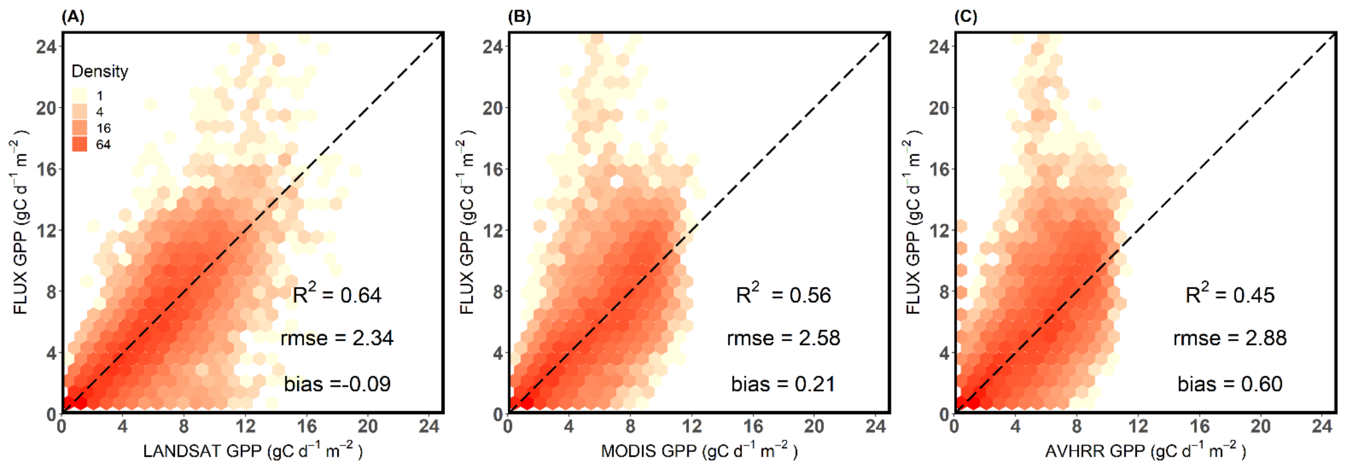
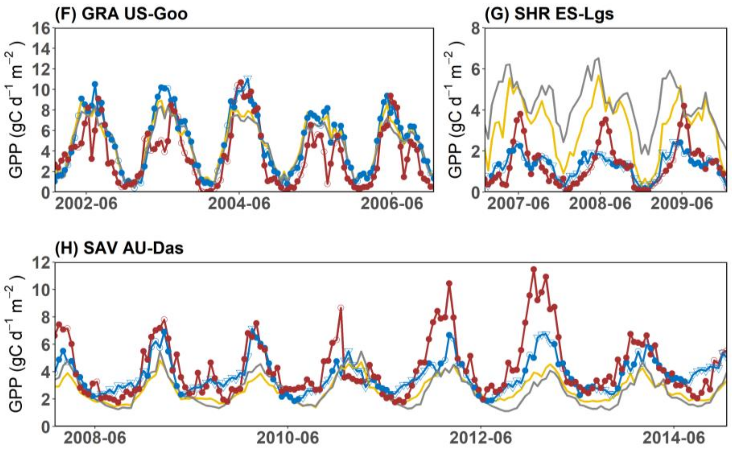
3.1. Evaluation of Fine Resolution GPP

The fine-spatial-resolution GPP (GPPL) correlated well with GPP measured from 193 eddy covariance towers (GPPFLUX) (Figure 3A). Overall, the GPPL had a coefficient of determination (R2) of around 0.64 and its RMSE was 2.34 g C m2 d−1. For the single vegetation type, the GPPL had a high level of agreement (R2 > 0.5) with the GPPFLUX for eight vegetation types, excluding the EBF (Table 4). Moreover, the GPPL had a low bias (<1 g C m−2 d−1) with the GPPFLUX at all the selected sites among vegetation types. The GPPL captured the seasonal profiles of the GPPFLUX at the typical sites of each vegetation type (Figure 4). For the forest stands, the GPPL tracked the seasonal change in GPP well in the selected sites. In particular, the GPPL showed similar seasonal profiles to the EBF stand. At the non-forest stands, the GPPL also captured the magnitude of the GPPFLUX. The GPPL tracked the GPPFLUX well at the savanna site, except at the peak of the growing season (Figure 4H).

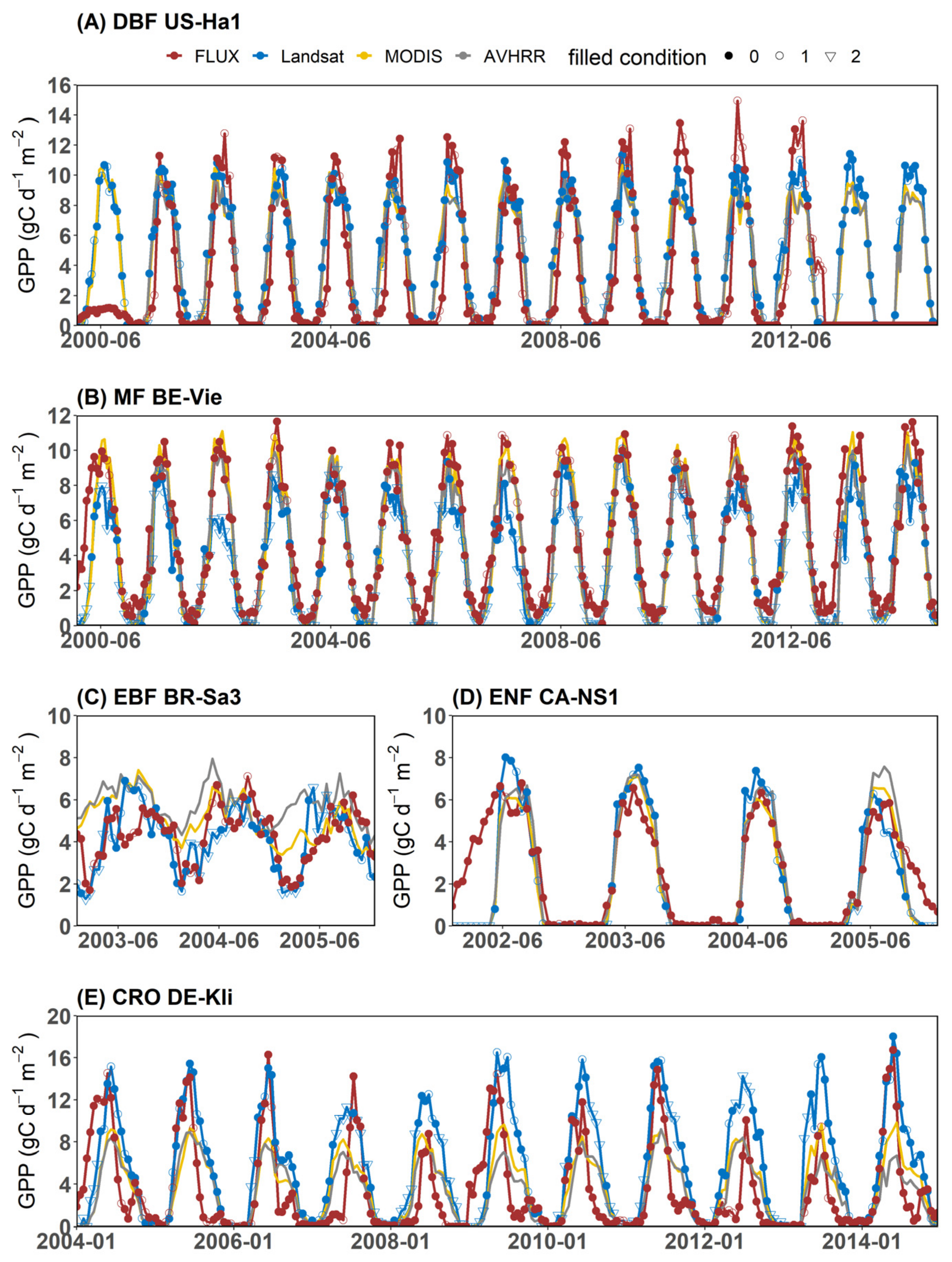
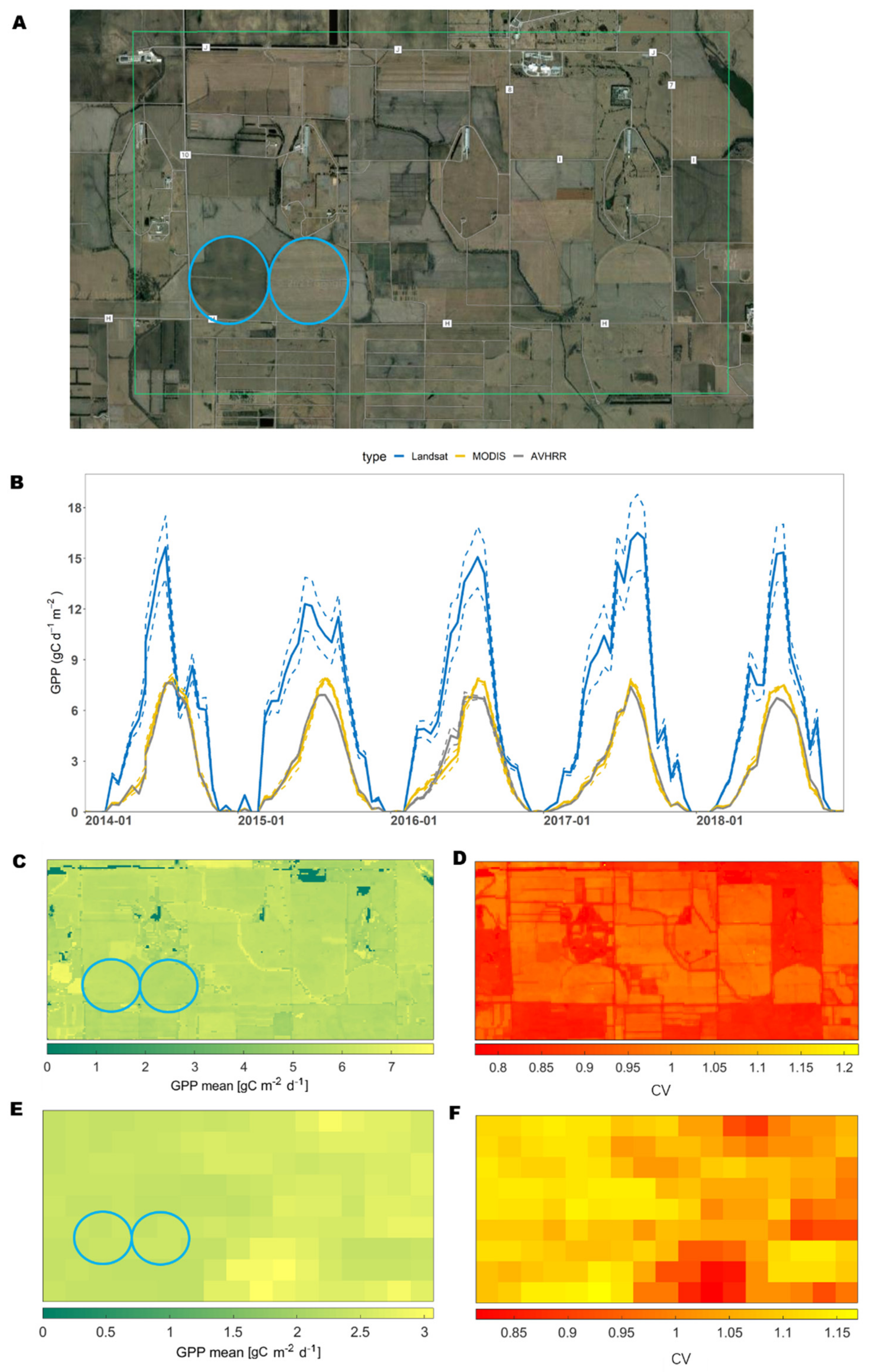
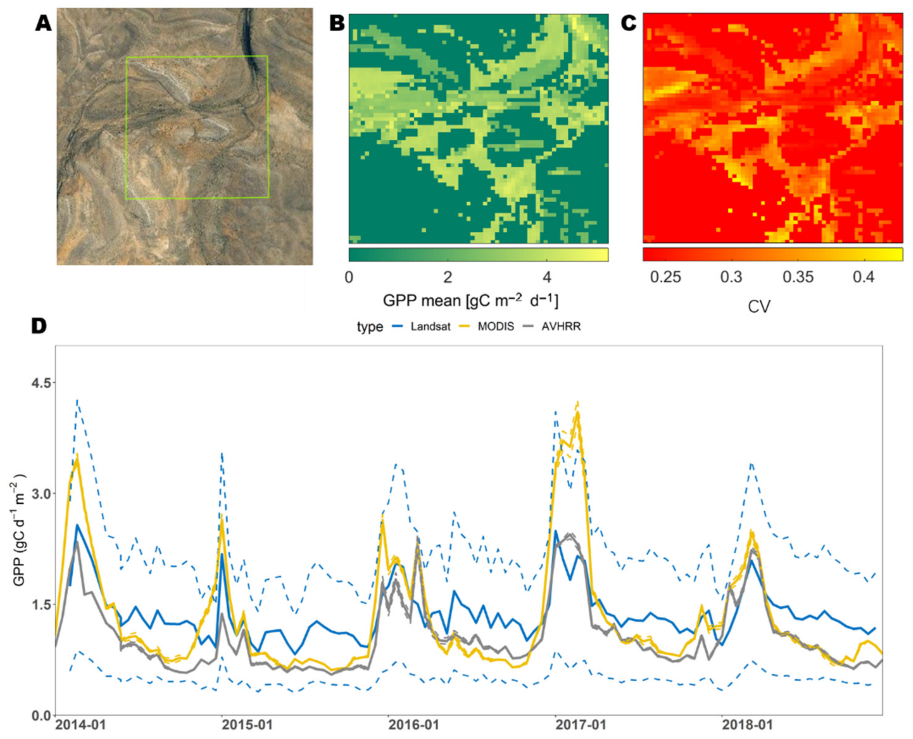
3.2. Comparison of GPP Estimates at Three Spatial Resolutions

In order to derive the intercomparison results from the three resolution GPP products, we compared 193 sites’ GPPFLUX with three resolutions of GPP product in constant dates. Compared to the other coarse-resolution GPP products (Figure 2), the GPPL had higher R2 and lower RMSE than the GPPM (R2 = 0.56, RMSE = 2.58 g C m−2 d−1) driven by the 500-meter-spatial-resolution MODIS data. The GPPA driven by the 0.05°AVHRR data had the lowest accuracy, with an R2 equal to 0.45 and an RMSE equal to 2.88 g C m−2 d−1. Moreover, the GPPL showed the least bias (−0.09 g C m−2 d−1) compared to the GPPM (0.21 g C m−2 d−1) and the GPPA (0.60 g C m−2 d−1). Most of the observed and modeled GPP were close to the 1:1 line. The GPPL showed higher R2 than the GPPM and GPPA in five of the nine individual vegetation types (Table 4). The GPPL significantly improved the GPP modeling, especially for cropland, savanna, and wetland, explaining more than 16%, 6%, and 16% of the variance in the coarse-spatial-resolution GPP, respectively. The GPPL also corrected the high bias of the GPP (>1 g C m−2 d−1) for cropland and shrub in the GPPM and GPPA. The coarse-spatial-resolution GPP (GPPM, GPPA) also followed the seasonal change in the GPP but could not reproduce the low GPP of January (Figure 4C). For the dryland vegetation types (SHR, SAV), however, the GPPM and GPPA were not able to reproduce the seasonal cycle of the GPPFLUX. The GPPM and GPPA showed overestimations of GPP in the Mediterranean dryland (Figure 4G)
The GPPL captured the spatial and temporal change in GPP better than the coarse-resolution GPP in agroecosystems (Figure 5). The coarse-resolution GPP (GPPM and GPPA) showed less spatial variance than the fine-resolution GPP. The highest standard deviation of the GPP (GPPSTD) in the GPPL occurred in August 2017 (4.561 g C m−2 d−1). At the same time, the GPPM and GPPA had a GPPSTD of 0.381 and 0.045 g C m−2 d−1, respectively (Figure 5B). Moreover, the GPPL during the peak of the growing season (~17 g C m−2 d−1) was much higher than the GPPM (~9 g C m−2 d−1) and GPPA (~9 g C m−2 d−1). The GPPL also showed that the annual mean GPP was higher in the irrigated regions (blue circles in Figure 5A,C,E) compared to the GPPM. Overall, the GPPL reproduced the GPP (0 g C m−2 d−1 at some northern pixels) of roads and non-planted areas (Figure 5C), but the GPPM did not indicate these conditions (Figure 5E). The fine-spatial-resolution GPP also characterized the spatial heterogeneity of the seasonal change in GPP. The GPPL showed that the overall CV of the GPP ranged from 0.75 to 1.23 in this region, but the GPPM showed that the CV of the GPP ranged from 0.81 to 1.16. In the irrigated region, the highest CVs of the GPPL and GPPM were 1.2 and 1.15, respectively (Figure 5D,F). Moreover, the GPPM showed almost no significant spatial difference in this region.
Dryland ecosystems include savanna, open shrubland, and deserts. In savanna ecosystems, the landscape includes random areas of grass and trees, which leads to high spatial heterogeneity in the GPP. Although the mean values of the GPP were similar to the GPPL, GPPM, and GPPA at the research site (Figure 6), the spatial variance in the GPP was quite different. The GPPL showed the highest GPPSTD, of around 3.378 g C m−2 d−1, while the GPPSTD in the GPPM and GPPA were 0.134 and 0.005 g C m−2 d−1, respectively (Figure 6D). The seasonal variations in the GPP showed different patterns (Figure 6C) of pixels representing trees (CV ~0.25) and pixels predominantly representing grass (CV~0.4). For the desert, the GPPL captured the seasonal change in GPP in an oasis (Figure 7). However, since the GPP driven by MODIS data misclassified the vegetation type in this region, the GPP in this region was close to zero. The GPPM had a maximum GPP of only around 0.002 g C m−2 d−1 in 2016, which suggested a significant underestimation compared to the GPPL.

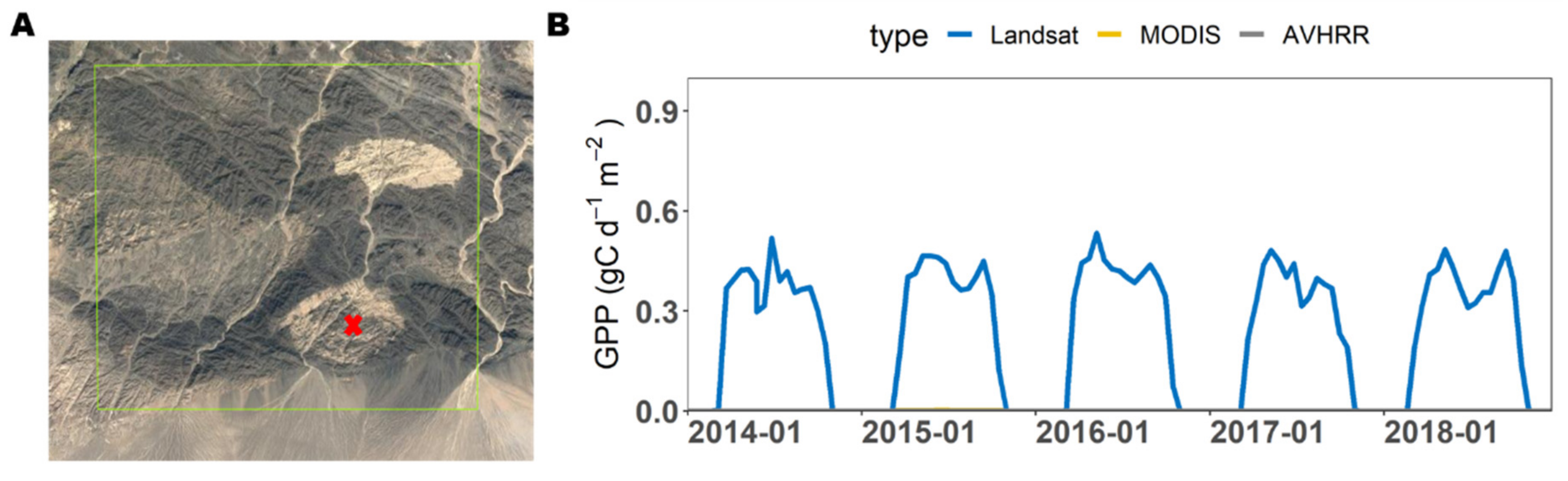
3.3. The Acquisition of Landsat Data Affects GPP Estimation

The data acquisition of Landsat NDVI strongly affected the fine-spatial-resolution GPP modeling accuracy. Figure 8A shows that the proportions of cloud-free NDVI observations in the total data acquisition ranged from 26% to 43% over all nine ecosystem types. The DBF, SHR, and WET had higher proportions (>40%) of cloud-free NDVI observations than the other vegetation types. A low proportion of cloud-free NDVI was found in CRO and EBF, and therefore, more than 56% of the periods of the NDVI values were reconstructed. In each vegetation type, the RPE in the GPPL based on observed NDVI (GPPL0) and the GPPL based on the reconstructed NDVI from short-term gap-filling (GPPL1) were similar (Figure 8B), ranging from -5% (ENF) to 22% (CRO). Conversely, the RPE in the GPPL based on reconstructed NDVI from long-term gap-filling (GPPL2) was higher than the RPE of the GPPL0. Apart from the EBF, the lowest absolute RPE was 5% (DBF) and the highest was 49%, in the CRO. The differences between the GPPL0 and the GPPL2 were much greater (>30%) in the SHR and CRO than in the other vegetation types. The R2 was much higher in the GPPL0 than in the GPPL2 in most vegetation types (Figure 8C). Meanwhile, the RMSE was similar among the GPPL0, GPPL1, and GPPL2 (Figure 8D). This is because the mean value of the GPP was higher in the GPPL0 when it was under clear sky, and the incident PAR was much higher than the GPPL2 when it was under cloudy sky. Thus, the higher RMSE in the GPPL0 was not linked to higher uncertainties in the GPPL0 compared to the GPPL2. Generally, our results showed that the GPPL0 was less uncertain than the GPPL2 for most of the vegetation types.

4. Discussion

4.1. Benefits of the One-Step Process of GPP

In this study, we provided a web APP for generating fine-spatial-resolution (30-m) GPP (Figure A1), which allows users to derive the GPP at any given study area around the world. This tool can be used to obtain and download the GPP on demand, providing one-step GPP processing. This APP has three advantages: high efficiency, workload reduction, and open access. First, we used this APP to generate 15 years of fine-spatial-resolution GPP from 193 sites in less than 3 h. Second, since this APP reduces the workload by eliminating data download and image preprocessing, it easily obtains spatiotemporally continuous GPP simulations. Third, since GEE is an open-access platform, this APP can be accessed by all users. For specific applications, users can use this platform to compare the fine-spatial-resolution GPP to other data. This helps cross-comparisons of GPP models, as well as the comparison of GPP to any given bio-physiological variable (e.g., soil water content, ozone concentration). Specifically, to our knowledge, this is the first APP to provide access to fine-spatial-resolution GPPs for any selected location around the world. Therefore, with this APP, users can easily evaluate GPP changes, especially in heterogeneous regions such as deserts, savanna, and cropland.

4.2. Fine-Spatial-Resolution Remote Sensing Data Improves GPP Estimations

The fine-spatial-resolution GPP product (GPPL) showed good agreement with the GPP observed at the flux sites (Figure 3 and Figure 4; Table 4), which indicated that the GPPL could characterize the spatial and temporal change in GPP better than the coarse-spatial-resolution GPP products. The GPPL significantly improved the accuracy of the GPP simulations in the cropland and dryland ecosystems [20]. Our results suggested that the GPPL provided more detailed information with which to delineate the GPP distribution (Figure 5, Figure 6 and Figure 7). Fine-resolution images can be used to characterize the spatial heterogeneity of roads, buildings, farmland in cropland ecosystems, and grass and trees in savanna ecosystems. The improved consideration of the seasonal change in GPP in savanna may improve our understanding of its dynamic carbon sequestration [20,21]. Furthermore, the GPPL of evergreen broadleaf forest can represent the GPP decrease in the dry season better than coarse spatial GPP products (Figure 4C). Therefore, the GPPL characterizes the complexity of GPP [10] and supports specific applications in spatially heterogeneous regions [4].
The GPPL represented the magnitude of the GPP because we reparametrized the coefficients in the fine-spatial-resolution EC-LUE model. On the one hand, Nguy-Robertson et al. (2015) reported that at the Nebraska extension cropland experiment site (Figure 5) [22], the maximal daily GPP of soybean could reach 18 g C m−2 d−1, but both the GPPM and the GPPA significantly underestimated this condition. After optimizing the coefficients in the EC-LUE model, the peak of the GPPL was 17.5 g C m−2 d−1, which was close to the observed GPP [8]. Thus, using the GPPL to evaluate the amount of GPP in a cropland area can better characterize the growing condition of crops and precisely estimate their yield [23]. On the other hand, in desert regions, vegetation begins to grow after rainfall, but its distribution is sparse. The land-cover classification in coarse-spatial-resolution data may identify these areas as non-vegetated, so the GPP is set to zero. However, fine-spatial-resolution data can be used to detect very small changes in vegetation growth, as indicated by NDVI, in the form of pixels covered by vegetation [24]. Moreover, although the total amount of GPP in dryland may be lower, its expansion leads to substantial changes in GPP [25]. Therefore, the GPPL product can precisely simulate the total amount of photosynthesis over a large region.

4.3. Challenges and Future Work

Even though the fine-spatial-resolution GPP can reflect the spatial heterogeneity of the GPP, its modeling accuracy is affected by the acquisition of remote sensing data. Unlike the coarse-spatial-resolution remote sensing data, which have more than two observations at any given location of the land surface each day, the Landsat series satellite produces sparse observations. On average, for each Landsat satellite had 23 observations at the same location each year, but due to cloud cover, 50% of the cloud-free data were missing [14,15,26]. Our results showed that the total amount of reconstructed NDVI based on the long-term gap-filling method is around 50% for most of the vegetation types (Figure 8A), which leads to high uncertainties in the GPPL (Figure 8B). Similarly, a recent study showed that around 50% of Landsat data are cloud-covered, leading to uncertainties in crop yield estimations [27,28].
This indicates that the modeling accuracy of fine-spatial-resolution GPP is highly affected by the data gaps in the time series of fine-spatial-resolution remote sensing data. There are some solutions for this: first, different sources of fine-scale data can be harmonized, such as in the harmonization of Landsat and Sentinel-2 data [29], but this approach is limited by the shorter availability of Sentinel-2 data; second, researchers use data fusion methods with coarse-spatial-resolution remote sensing data [30,31], as in the case of MODIS-Landsat data generation, but this approach requires the recalibration of the reflectance at each channel [32,33]; third, researchers use a data assimilation method to generate Landsat time-series data with climate data [34], but this approach needs huge amounts of computing resources, so it is not available for large-scale evaluation on the cloud platform. Therefore, future work on mapping the GPP on a continental scale should apply fine-scale spatio-temporally reconstructed cloud-free remote sensing data.

5. Conclusions

We presented a web application for generating fine-spatial-resolution GPP driven by 30-m Landsat time-series data (i.e., GPPL). The GPPL precisely characterized the spatial heterogeneity and the seasonal variations in the GPP of complex landscapes, while the coarse-spatial-resolution remote sensing data could not reproduce these conditions. Significant improvements in GPPL were found in agroecosystems and dryland ecosystems, such as shrubland and savanna, compared to the coarse-spatial-resolution GPP products. The EC-LUE model driven by fine spatial resolution with optimized coefficients also corrected the GPP estimation biases for the cropland and dryland, which could be used to reproduce the total amount of plant photosynthesis. Furthermore, the acquisition of the Landsat data strongly affected the estimation accuracy of the GPPL. Therefore, future work should apply spatio-temporally continuous reconstructed fine-spatial-resolution remote sensing data to the GPP product. Furthermore, since the land-cover map on the GEE platform changes every five years, future work on GPP mapping should apply the dynamic land-cover map, which can capture the GPP changes caused by annual land cover changes. With our online APP on GEE, users can generate GPP at any given location and for any year since 1984 on demand. This will help with the development of further applications that investigate the relationship between GPP and other parameters.

Author Contributions

Conceptualization, S.L. and W.Y.; methodology, X.H., Y.Z. and X.Z.; software, S.L. and X.Z.; validation, S.L. and X.H.; resources, Y.Z.; writing—original draft preparation, S.L. and W.Y.; writing—review and editing, S.L., Y.Z. and W.Y.; visualization, S.L.; funding acquisition, S.L. and W.Y. All authors have read and agreed to the published version of the manuscript.

Funding

This research was funded by National Natural Science Foundation of China, grant number No. 42141020, National Natural Science Foundation of China, grant number No. 42101319, China Postdoctoral Science Foundation Funded Project, grant number 2021M703658, and the Fundamental Research Funds for the Central Universities, Sun Yet-sen University (2021qntd29). The APC was funded by China Postdoctoral Science Foundation Funded Project (2021M703658).

Acknowledgments

This work used eddy covariance data acquired and shared by the FLUXNET community, including the following networks: AmeriFlux, AfriFlux, AsiaFlux, CarboAfrica, CarboEuropeIP, CarboItaly, CarboMont, ChinaFlux, Fluxnet-Canada, GreenGrass, ICOS, KoFlux, LBA, NECC, OzFlux-TERN, Swiss FluxNet, TCOS-Siberia, and USCCC. The ERA-Interim reanalysis data were provided by ECMWF and processed by LSCE. The FLUXNET eddy covariance data processing and harmonization was carried out by the European Fluxes Database Cluster, AmeriFlux Management Project, and the Fluxdata project of FLUXNET, with the support of CDIAC and ICOS Ecosystem Thematic Center, and the OzFlux, ChinaFlux, and AsiaFlux offices. This work was also supported by the Ministry of Education, Youth and Sports of the Czech Republic within the National Sustainability Programme I (NPU I), grant number LO1415 and by the project for national infrastructure support CzeCOS/ICOS, reg. no. LM2015061.

Conflicts of Interest

The authors declare no conflict of interest.

Appendix A

The online APP is available at the following link: https://shangrong-lin.users.earthengine.app/view/ec-lue-gpp-landsat-v0, accessed on 19 May 2022.
Figure A1. Platform image.
Remotesensing 14 02651 g0a1

References

  1. Yuan, W.; Cai, W.; Xia, J.; Chen, J.; Liu, S.; Dong, W.; Merbold, L.; Law, B.; Arain, A.; Beringer, J.; et al. Global comparison of light use efficiency models for simulating terrestrial vegetation gross primary production based on the LaThuile database. Agric. For. Meteorol. 2014, 192–193, 108–120. [Google Scholar] [CrossRef]
  2. Lin, S.; Li, J.; Liu, Q.; Gioli, B.; Paul-Limoges, E.; Buchmann, N.; Gharun, M.; Hörtnagl, L.; Foltýnová, L.; Dušek, J.; et al. Improved global estimations of gross primary productivity of natural vegetation types by incorporating plant functional type. Int. J. Appl. Earth Obs. Geoinf. ITC J. 2021, 100, 102328. [Google Scholar] [CrossRef]
  3. Zheng, Y.; Shen, R.; Wang, Y.; Li, X.; Liu, S.; Liang, S.; Chen, J.M.; Ju, W.; Zhang, L.; Yuan, W. Improved estimate of global gross primary production for reproducing its long-term variation, 1982–2017. Earth Syst. Sci. Data 2020, 12, 2725–2746. [Google Scholar] [CrossRef]
  4. Gelybó, G.; Barcza, Z.; Kern, A.; Kljun, N. Effect of spatial heterogeneity on the validation of remote sensing based GPP estimations. Agric. For. Meteorol. 2013, 174–175, 43–53. [Google Scholar] [CrossRef]
  5. Chen, B.; Ge, Q.; Fu, D.; Yu, G.; Sun, X.; Wang, S.; Wang, H. A data-model fusion approach for upscaling gross ecosystem productivity to the landscape scale based on remote sensing and flux footprint modelling. Biogeosciences 2010, 7, 2943–2958. [Google Scholar] [CrossRef] [Green Version]
  6. Huang, X.; Zheng, Y.; Zhang, H.; Lin, S.; Liang, S.; Li, X.; Ma, M.; Yuan, W. High spatial resolution vegetation gross primary production product: Algorithm and validation. Sci. Remote Sens. 2022, 5, 100049. [Google Scholar] [CrossRef]
  7. Xie, X.; Li, A. An Adjusted Two-Leaf Light Use Efficiency Model for Improving GPP Simulations Over Mountainous Areas. J. Geophys. Res. Atmos. 2020, 125, 1–19. [Google Scholar] [CrossRef]
  8. Gitelson, A.A.; Peng, Y.; Masek, J.G.; Rundquist, D.C.; Verma, S.; Suyker, A.; Baker, J.M.; Hatfield, J.L.; Meyers, T. Remote estimation of crop gross primary production with Landsat data. Remote Sens. Environ. 2012, 121, 404–414. [Google Scholar] [CrossRef] [Green Version]
  9. Balzarolo, M.; Peñuelas, J.; Veroustraete, F. Influence of Landscape Heterogeneity and Spatial Resolution in Multi-Temporal In Situ and MODIS NDVI Data Proxies for Seasonal GPP Dynamics. Remote Sens. 2019, 11, 1656. [Google Scholar] [CrossRef] [Green Version]
  10. Robinson, N.P.; Allred, B.W.; Smith, W.K.; Jones, M.O.; Moreno, A.; Erickson, T.A.; Naugle, D.E.; Running, S.W. Terrestrial primary production for the conterminous United States derived from Landsat 30 m and MODIS 250 m. Remote Sens. Ecol. Conserv. 2018, 4, 264–280. [Google Scholar] [CrossRef]
  11. Wulder, M.A.; Loveland, T.R.; Roy, D.P.; Crawford, C.J.; Masek, J.G.; Woodcock, C.E.; Allen, R.G.; Anderson, M.C.; Belward, A.S.; Cohen, W.B.; et al. Current status of Landsat program, science, and applications. Remote Sens. Environ. 2019, 225, 127–147. [Google Scholar] [CrossRef]
  12. Yuan, W.; Zheng, Y.; Piao, S.; Ciais, P.; Lombardozzi, D.; Wang, Y.; Ryu, Y.; Chen, G.; Dong, W.; Hu, Z.; et al. Increased atmospheric vapor pressure deficit reduces global vegetation growth. Sci. Adv. 2019, 5, eaax1396. [Google Scholar] [CrossRef] [PubMed] [Green Version]
  13. Liang, S.; Cheng, J.; Jia, K.; Jiang, B.; Liu, Q.; Xiao, Z.; Yao, Y.; Yuan, W.; Zhang, X.; Zhao, X.; et al. The Global Land Surface Satellite (GLASS) Product Suite. Bull. Am. Meteorol. Soc. 2021, 102, E323–E337. [Google Scholar] [CrossRef]
  14. Ju, J.; Roy, D.P. The availability of cloud-free Landsat ETM+ data over the conterminous United States and globally. Remote Sens. Environ. 2008, 112, 1196–1211. [Google Scholar] [CrossRef]
  15. Zhu, Z.; Woodcock, C.E.; Holden, C.; Yang, Z. Generating synthetic Landsat images based on all available Landsat data: Predicting Landsat surface reflectance at any given time. Remote Sens. Environ. 2015, 162, 67–83. [Google Scholar] [CrossRef]
  16. Roy, D.P.; Kovalskyy, V.; Zhang, H.K.; Vermote, E.F.; Yan, L.; Kumar, S.S.; Egorov, A. Characterization of Landsat-7 to Landsat-8 reflective wavelength and normalized difference vegetation index continuity. Remote Sens. Environ. 2016, 185, 57–70. [Google Scholar] [CrossRef] [PubMed] [Green Version]
  17. Zhang, X.; Liu, L.; Chen, X.; Gao, Y.; Xie, S.; Mi, J. GLC_FCS30: Global land-cover product with fine classification system at 30 m using time-series Landsat imagery. Earth Syst. Sci. Data 2021, 13, 2753–2776. [Google Scholar] [CrossRef]
  18. Pastorello, G.; Trotta, C.; Canfora, E.; Chu, H.; Christianson, D.; Cheah, Y.; Poindexter, C.; Chen, J.; Elbashandy, A.; Humphrey, M.; et al. The FLUXNET2015 dataset and the ONEFlux processing pipeline for eddy covariance data. Sci. Data 2020, 7, 225. [Google Scholar] [CrossRef]
  19. Huang, X.; Xiao, J.; Wang, X.; Ma, M. Improving the global MODIS GPP model by optimizing parameters with FLUXNET data. Agric. For. Meteorol. 2021, 300, 108314. [Google Scholar] [CrossRef]
  20. Abreu, R.C.R.; Hoffmann, W.A.; Vasconcelos, H.L.; Pilon, N.A.; Rossatto, D.R.; Durigan, G. The biodiversity cost of carbon sequestration in tropical savanna. Sci. Adv. 2017, 3, e1701284. [Google Scholar] [CrossRef] [Green Version]
  21. Grace, J.; Jose, J.S.; Meir, P.; Miranda, H.; Montes, R.A. Productivity and carbon fluxes of tropical savannas. J. Biogeogr. 2006, 33, 387–400. [Google Scholar] [CrossRef]
  22. Nguy-Robertson, A.; Suyker, A.; Xiao, X. Modeling gross primary production of maize and soybean croplands using light quality, temperature, water stress, and phenology. Agric. For. Meteorol. 2015, 213, 160–172. [Google Scholar] [CrossRef] [Green Version]
  23. Dong, J.; Lu, H.; Wang, Y.; Ye, T.; Yuan, W. Estimating winter wheat yield based on a light use efficiency model and wheat variety data. ISPRS J. Photogramm. Remote Sens. 2019, 160, 18–32. [Google Scholar] [CrossRef]
  24. Villarreal, M.L.; Norman, L.M.; Buckley, S.; Wallace, C.S.; Coe, M.A. Multi-index time series monitoring of drought and fire effects on desert grasslands. Remote Sens. Environ. 2016, 183, 186–197. [Google Scholar] [CrossRef] [Green Version]
  25. Yao, J.; Liu, H.; Huang, J.; Gao, Z.; Wang, G.; Li, D.; Yu, H.; Chen, X. Accelerated dryland expansion regulates future variability in dryland gross primary production. Nat. Commun. 2020, 11, 1665. [Google Scholar] [CrossRef] [Green Version]
  26. Yan, L.; Roy, D.P. Spatially and temporally complete Landsat reflectance time series modelling: The fill-and-fit approach. Remote Sens. Environ. 2020, 241, 111718. [Google Scholar] [CrossRef]
  27. Dong, J.; Fu, Y.; Wang, J.; Tian, H.; Fu, S.; Niu, Z.; Han, W.; Zheng, Y.; Huang, J.; Yuan, W. Early-season mapping of winter wheat in China based on Landsat and Sentinel images. Earth Syst. Sci. Data 2020, 12, 3081–3095. [Google Scholar] [CrossRef]
  28. Fu, Y.; Huang, J.; Shen, Y.; Liu, S.; Huang, Y.; Dong, J.; Han, W.; Ye, T.; Zhao, W.; Yuan, W. A Satellite-Based Method for National Winter Wheat Yield Estimating in China. Remote Sens. 2021, 13, 4680. [Google Scholar] [CrossRef]
  29. Claverie, M.; Ju, J.; Masek, J.G.; Dungan, J.L.; Vermote, E.F.; Roger, J.-C.; Skakun, S.V.; Justice, C. The Harmonized Landsat and Sentinel-2 surface reflectance data set. Remote Sens. Environ. 2018, 219, 145–161. [Google Scholar] [CrossRef]
  30. Zhou, F.; Zhong, D. Kalman filter method for generating time-series synthetic Landsat images and their uncertainty from Landsat and MODIS observations. Remote Sens. Environ. 2020, 239, 111628. [Google Scholar] [CrossRef]
  31. Li, X.; Yuan, W.; Dong, W. A Machine Learning Method for Predicting Vegetation Indices in China. Remote Sens. 2021, 13, 1147. [Google Scholar] [CrossRef]
  32. Steven, M.D.; Malthus, T.J.; Baret, F.; Xu, H.; Chopping, M.J. Intercalibration of vegetation indices from different sensor systems. Remote Sens. Environ. 2003, 88, 412–422. [Google Scholar] [CrossRef]
  33. Masek, J.G.; Gao, F.; Wolfe, R.; Huang, C. Building a consistent medium resolution satellite data set using moderate resolution imaging spectroradiometer products as reference. J. Appl. Remote Sens. 2010, 4, 043526. [Google Scholar] [CrossRef]
  34. Yu, W.; Li, J.; Liu, Q.; Zhao, J.; Dong, Y.; Zhu, X.; Lin, S.; Zhang, H.; Zhang, Z. Gap Filling for Historical Landsat NDVI Time Series by Integrating Climate Data. Remote Sens. 2021, 13, 484. [Google Scholar] [CrossRef]
Figure 1. Workflow for generating fine-spatial-resolution GPP by the EC-LUE model.
Remotesensing 14 02651 g001
Figure 2. Workflow of reconstructed NDVI.
Remotesensing 14 02651 g002
Figure 3. Three-spatial-resolution GPP data compared to GPP observed at flux sites. The three series of GPP data: Landsat (A), MODIS (B), and AVHRR (C) were consistent with the date at 16-day intervals. The dashed line is the 1:1 line.
Remotesensing 14 02651 g003
Figure 4. Time series of GPP (flux), GPPL (Landsat), GPPM (MODIS), and GPPA (AVHRR) at eight typical vegetation sites. The symbols ●, ○, and ▽ in GPPL represent the GPP driven by observed short-term gap-filled reconstructed NDVI and long-term gap-filled reconstructed NDVI, respectively. The symbols ● and ○ in the flux-tower-based GPP (red curve) are the observed GPP and gap-filled GPP, respectively.
Remotesensing 14 02651 g004aRemotesensing 14 02651 g004b
Figure 5. A typical agroecosystem near Mead, Nebraska, USA (41.1651 N, 96.4766 W). The research area is in the green box of subplot (A). Subplot (B) shows the seasonal change in GPPL, GPPM, and GPPA from 2014–2018. The dashed line represents the standard deviation of each pixel GPP in the research area. Subplots (C,E) are the mean GPP for five years of each pixel from GPPL and GPPM, respectively. Subplots (D,F) are the temporal change in GPP, which is quantified by the coefficient of variation (CV) of each pixel.
Remotesensing 14 02651 g005
Figure 6. A savanna ecosystem near Gregory, Queensland, Australia (139.34 E, 18.89 S). The research region is in the green box of subplot (A). Subplots (B,C) show the mean GPP and seasonal change in GPP at each pixel from 2014 to 2018, respectively. Subplot (D) shows the seasonal change in GPPL, GPPM, and GPPA, while the dashed curves represent the ±1 standard deviation of GPP in the entire research region in each series.
Remotesensing 14 02651 g006
Figure 7. Subplot (A) shows an oasis in the desert at Qiancaozi, Xinjiang, China (94.65°E, 42.63°N). Subplot (B) shows the seasonal change in GPPL, GPPM, and GPPA, while the GPPM and GPPA are close to 0 at the red cross representing an oasis (Figure 7A).
Remotesensing 14 02651 g007
Figure 8. (A) Proportion of three types of reconstructed NDVI data and (B) relative prediction error (RPE), (C) R2, and (D) RMSE of GPP driven by different reconstructed NDVI among nine vegetation types. All the NDVI and GPP data were collected from the 193 investigated sites.
Remotesensing 14 02651 g008aRemotesensing 14 02651 g008b
Table 1. Data quality tag of gap-filled and reconstructed NDVI.
Quality DefinitionData Gap (x in days) between Two
Nearest Observed NDVI in
16 Days Intervals
QCtagNDVI-Filled Method
Reconstructed NDVI based on observation00Not applied
Reconstructed NDVI based on short-term gap-filling0 < x ≤ 481Linearly interpolated from the nearest two available NDVI
Reconstructed NDVI based on long-term gap-filling48 < x2Linearly interpolated from the nearest two available NDVI
Table 2. Data sources for generating GPP on the GEE platform.
DataSpecific NameTransferred
Unit
Spatial
Resolution
Data Source or Reference
NDVINormalized-difference vegetation indexUnitless30 mThis study
Shortwave radiationDownward short-wave radiation Flux surface 6-h averageMJ m−2 day−10.5°NCEP
Surface pressureSurface pressurePa0.5°NCEP
2-m air temperatureMean 2-m air temperature°C0.25°ERA5
2-m dewpoint temperatureDewpoint 2-m temperature°C0.25°ERA5
CO2Global monthly mean CO2ppm/https://gml.noaa.gov/ccgg/trends/gl_trend.html, accessed on 31 December 2021
Vegetation classification mapGLC-FCS30 30 m[17]
Table 3. Model coefficients of the fine-spatial-resolution GPP from the GEE APP. Model coefficients are linked to Equations (1), (4) and (5).
Vegetation Typeεmax (g C m−2 MJ−1) ϑ VPD0 (kPa)
DBF3.2671.091.16
EBF2.5049.420.94
ENF2.8945.690.81
MF2.9366.870.86
GRA3.3770.111.05
SAV2.3353.241.89
SHR1.2337.211.30
WET2.9476.791.28
CRO4.5064.001.50
Table 4. GPP validation for different vegetation types. Bold indicates the best statistic. The unit of RMSE and bias is g C m−2 d−1.
Landsat
R2
MODIS
R2
AVHRR
R2
Landsat
RMSE
MODIS RMSEAVHRR
RMSE
Landsat
bias
MODIS
bias
AVHRR
bias
CRO0.530.370.404.845.595.47−0.813.083.28
DBF0.730.720.612.382.392.85−0.31−0.030.74
EBF0.310.350.402.392.332.240.52−0.070.32
ENF0.660.710.411.801.672.38−0.140.110.59
GRA0.620.630.522.312.282.61−0.080.410.80
MF0.650.650.641.981.972.010.16−0.53−0.44
SAV0.720.660.501.331.461.78−0.020.690.78
SHR0.700.680.510.971.011.240.11−1.35−1.62
WET0.600.440.502.182.592.46−0.01−0.06−0.17
Publisher’s Note: MDPI stays neutral with regard to jurisdictional claims in published maps and institutional affiliations.

