A Nyström-Based Low-Complexity Algorithm with Improved Effective Array Aperture for Coherent DOA Estimation in Monostatic MIMO Radar

Abstract

In this paper, we propose a computationally efficient algorithm with improved effective aperture for coherent angle estimation in a monostatic multiple-input multiple-output (MIMO) radar. First, the direction matrix of MIMO radar is mapped into a low-dimensional matrix of virtual uniform linear array (ULA). Then, an augmented data expansion matrix with improved effective aperture is obtained by exploiting the Vandermonde-like structure of the low-dimensional direction matrix and radar cross section (RCS) matrix to enlarge the aperture of the array. Next, a unitary transformation is used to transform the augmented matrix into a real value and the approximate signal subspace of the augmented matrix is obtained by the Nyström method, which can reduce the computational complexity. The eigenvectors of the approximate signal subspace are used to reconstruct the matrix for direct decorrelation processing. Finally, direction of arrivals (DOAs) can be estimated faster by utilizing the unitary ESPRIT algorithm since the rotation invariance of the extended reconstruction matrix still exists. The proposed algorithm has a lower total computational complexity, and the estimation accuracy is improved by utilizing real values and enlarging the array aperture for estimation. Several theoretical analyses and simulation results confirm the effectiveness and advantages of the proposed method.

1. Introduction

As a new radar system, the multiple-input multiple-output (MIMO) radar was developed by combining MIMO communication technology with digital array technology [1]. Due to its excellent detection performance, it has attracted increasing attention in recent years. For the MIMO radar, the transmitter emits orthogonal waveforms, and different transmitting and receiving array arrangements are utilized, which leads to waveform diversity and spatial diversity to obtain better detection and estimation performance than the phase-array radar [2]. The MIMO radar can be grouped into two classes based on the spacing of each element in the transmitting and receiving antenna array. One is called the colocated MIMO radar [3]; the other is the statistical MIMO radar [4]. The spacing of the transmitting and receiving antennas in the colocated MIMO radar is generally close. It can obtain a virtual aperture that is larger than the real aperture, which creates advantages such as a narrower beamwidth, higher angular resolution, and angular estimation accuracy [3]. The colocated MIMO radar can be classified into a bistatic and monostatic MIMO radar based on whether the transmitting and receiving arrays are placed in the same place. The statistical MIMO radar takes advantage of widely spaced transmitting/receiving antennas to achieve spatial diversity to solve the target scintillation problem [4]. Although the statistical MIMO radar has better target detection and parameter estimation performance than the colocated MIMO radar, the engineering implementation of the statistical MIMO radar is challenging. The colocated MIMO radar structure is easier to implement in engineering and has a wider practical application [5].

Angle estimation (i.e., the direction of arrival (DOA) and the direction of departure (DOD)) is one of the important issues for the MIMO radar to obtain target information. In the past decade, various methods have been proposed. For example, high-resolution subspace-based algorithms in array signal processing are applied in the MIMO radar, such as multiple signal classification (MUSIC) [6,7] and estimation signal parameters via rotational invariance techniques (ESPRIT) [8,9]. These algorithms can provide a better estimation performance for uncorrelated signals. Usually, MUSIC has a heavy computational burden owing to the spectrum searching. In order to avoid spectrum searching, some MUSIC variants are proposed and applied in the MIMO radar, such as Root-MUSIC [10]. This reduces complexity via computing the roots of the polynomials of a spatial spectrum. To further reduce the computational complexity, unitary transformation is used to convert complex-valued operations into real-valued operations, such as UMUSIC [11] or URoot-MUSIC [12]. The ESPRIT algorithm also avoids spectrum searching but is subject to certain array configuration requirements and somewhat reduces the array’s degrees of freedom (DOF). Thus, its performance is a little worse than that of MUSIC and its variants. Unitary transformation can also be used for ESPRIT, such as unitary ESPRIT. However, the above algorithms need to calculate the covariance and its eigen-decomposition of all the matched filtered outputs to obtain the signal or noise subspace for the angle estimation. Hence, these subspace-based algorithms are still rather computationally expensive, especially when the array size is large or receives a large number of pulses, which are not conducive to real-time signal processing. Moreover, the maximum-likelihood (ML) method [13] and methods based on compressive sensing (CS) [14] or tensors that were proposed [15] in recent years can also be applied in the MIMO radar. Although these algorithms can provide better performance, the ML method has a high computational complexity and CS-based methods are still necessary for ‘off-grid’ problems [16]. Meanwhile, CS-based methods and some tensor-based methods are iterative solutions, whose computational complexity is still not lower.

In order to reduce the computational burden, some rapid parameter estimation methods are proposed. For example, the propagator method (PM) [17] and its variants [18], the multistage Wiener filtering (MSWF)-based method [19]. The signal subspace and noise subspace can be obtained indirectly by these methods, avoiding the direct eigen-decomposition of the matched filtered outputs’ covariance. However, the PM-based method has a better estimation performance only in the case of high signal-to-noise ratio (SNR) [20]. In addition, the reference signals should be known based on the MSWF method, which leads to a limitation on practical application. In recent years, a method called Nyström has been used for angle estimation in the array signal processing field [21,22,23]. It was originally applied in the field of kernel machine learning [24]. It could also be used to approximate the eigenvector of corresponding data in discrete space—that is, the matrix representation of the Nyström method. At present, the Nyström method is one of the most popular low-rank matrix approximation algorithms. The Nyström-based method for angle estimation can obtain the signal subspace without calculating the covariance of all the array outputs and its eigendecomposition. Instead, an equivalent approximate signal subspace is obtained from the partial block matrices of array outputs, which greatly reduces the computational complexity [25,26].

In the presence of coherent or highly correlated targets, some algorithms for angle estimation suffer serious performance degradation owing to the errors that exist in the signal subspace due to the rank loss of the covariance matrix of array outputs. To solve this problem, decorrelation processing is needed. The usual methods are spatial smoothing preprocessing (SSP) [27,28], Toeplitz-based methods [29,30], and Hankel matrix reconstruction [31]. In traditional array signal processing, the basic idea of SSP is to partition the total array into several groups containing overlapping subarrays and take the average of the subarray covariance matrices with restored full rank for decorrelation. The basic idea of Toeplitz or Hankel matrix reconstruction is to reconstruct the matrix by outputs; the rank of this matrix is only related to the DOAs of signals. The methods that are exploited in the MIMO radar are similar in traditional array signal processing. In contrast, the steering vectors for the MIMO radar are virtual steering vectors composed of the Kronecker product of the transmit and receive steering vectors. In [32], a transmission diversity smoothing method is proposed. In [33,34], forward spatial smoothing is exploited of the outputs for joint coherent DOA and Doppler frequency estimation. On the basis of [33], the PM is exploited to rapidly estimate the signal subspace, thus forming a low-complexity algorithm in [34]. In [35,36], two different schemes of joint transmission and reception diversity smoothing were proposed; these approaches lead to more covariance matrices being available for spatial smoothing operation, which results in a better estimation performance than the TDS method. Another difference is that, in [36], the array aperture is enlarged by exploiting the centrosymmetric property of the virtual direction matrix. In [37], a group of spatial difference smoothing (SDS) techniques in the MIMO radar were proposed to facilitate the angle estimation of coherent signals under unknown correlated noise. A recent study [38] proposed a smoothing matrix set (SMS) scheme, which performs transmission diversity smoothing to form transmission subvectors (TSVs) and then perform reception diversity smoothing for each TSV. That is, each TSV consists of some reception subvectors (RSVs). By rearranging the elements of the covariance submatrix of each TSV along the vertical direction, both the forward-only SMS (FO-SMS) and forward–backward SMS (FB-SMS) methods are derived. This scheme can be simply understood as exploiting multiple smoothing on transmission diversity and reception diversity for decorrelation. Although SSP and its variants for the MIMO radar [32,33,34,35,36,37,38] can provide a better decorrelation performance, part of the array aperture may be lost and the operations can be complicated. In addition, the CS-based method has the advantage of decorrelation and generally does not require additional preprocessing [39].

In this paper, a low-complexity algorithm based on the Nyström method with an improved effective array aperture for coherent DOA estimation in monostatic MIMO radar is proposed. First, the steering vectors of the monostatic MIMO radar can be transformed into low-dimensional vectors of virtual uniform linear array (ULA) due to the received signal property. Thus, the subsequent angle estimation operations are carried out in the low-dimensional signal space to reduce redundant calculation. Then, an augmented data matrix with an improved effective aperture is obtained thanks to the RCS matrix and a low-dimensional virtual direction matrix based on a Vandermonde-like structure. After that, unitary transformation is used to transform data into real valued data, and the approximate signal subspace of the augmented matrix is obtained by the Nyström method for lower computational complexity. Next, we directly reconstruct the matrix by the eigenvectors of the approximate signal subspace for decorrelation. Finally, the angle estimation can be calculated more quickly by utilizing the unitary ESPRIT algorithm, since the rotation invariance of the extended reconstruction matrix still exists. The proposed algorithm improves the estimation accuracy due to the expanded array aperture. Furthermore, our scheme makes full use of the Nyström method, which can rapidly obtain the approximate signal subspace, and directly uses the approximate eigenvectors for decorrelation processing. This makes the total algorithm much simpler and means it has a lower computational complexity.

Nomenclature: Bold capital letters, e.g., $\mathbf{X}$, and bold lowercase letters, e.g., $\mathbf{x}$, denote matrices and vectors, respectively. (·)^∗, (·)^T, (·)^H, (·)⁻¹ and (·)^† represent conjugate, transpose, conjugate-transpose, inverse, and pseudo-inverse, respectively. $\otimes ,\odot$ indicate the Kronecker product and Khatri-Rao product. $\mathrm{diag}(\cdot )$ represents the diagonalization operation. $\mathrm{angle}(\cdot )$ stands for the phase angles for each element of the array. ${\mathbf{I}}_K$ denotes a $K\times K$ identity matrix. ${\mathbf{\Pi }}_K$ denotes an antidiagonal identity matrix.

2. Monostatic MIMO Radar Echo Model

Considering the monostatic MIMO radar system configured with ULA: Assume that the transmitting array and the receiving array are in the same place and the space between the two arrays is so small that the receiving angle of the echo is almost the same as the transmitting angle of the transmitted wave to the target. Therefore, the direction of arrival (DOA) and the direction of departure (DOD) are both ${\theta }_K$. The structure of the monostatic MIMO radar is as shown in Figure 1; the transmitting and receiving antenna array adopt $M$ and $N$ elements that are all calibrated. The spacing of the array elements is $d=\lambda /2$, where $\lambda$ is the carrier wavelength. In the transmitter, each transmit antenna emits M orthogonal-coded waveforms, and the length of symbols per pulse duration is $Q$. Suppose there are $K$ far-field targets located in the directions ${\theta }_1,{\theta }_2,\dots ,{\theta }_K$. Echo signals reflected by the targets are collected by the receive antennas, and the reflection coefficients of the targets fulfil the Swerling model I. Consider a coherent processing interval (CPI) consisting of $L$ pulses. The received array signal at the $l\mathrm{-th} (l=1,2,\dots ,L)$ period can be expressed as follows [19,40]:

$${\mathbf{X}}_l={\mathbf{A}}_R\mathrm{diag}({\mathbf{b}}_l){\mathbf{A}}_T^T\mathbf{S}+{\mathbf{N}}_l,$$

(1)

where ${\mathbf{A}}_R=[{\mathbf{a}}_r({\theta }_1),{\mathbf{a}}_r({\theta }_2),\dots ,{\mathbf{a}}_r({\theta }_K)]\in {ℂ}^{N\times K}$ represents the receive direction matrix with the receive steering vectors given by ${\mathbf{a}}_r({\theta }_k)={[1,\dots ,e^{j\pi (N-1)\sin {\theta }_k}]}^T$; ${\mathbf{A}}_T=[{\mathbf{a}}_t({\theta }_1),{\mathbf{a}}_t({\theta }_2),\dots ,{\mathbf{a}}_t({\theta }_K)]\in {ℂ}^{M\times K}$ represents the transmit direction matrix with the transmit steering vectors given by ${\mathbf{a}}_t({\theta }_k)={[1,\dots ,e^{j\pi (M-1)\sin {\theta }_k}]}^T$; ${\mathbf{b}}_l={[{\alpha }_1{e}^{j2\pi l{f}_1/f_s},\dots ,{\alpha }_K{e}^{j2\pi l{f}_K/f_s}]}^T$ denotes the $l\mathrm{-th}$ echo coefficient vector. Here, ${\alpha }_k,f_k(k=1,2,\dots ,K)$ and $f_s$ represent the radar cross section (RCS) coefficients, the Doppler frequency, and the pulse repeat frequency, respectively. If the $K$ far-field sources are coherent, their Doppler frequency and RCS coefficients are assumed to be identical. $\mathbf{S}={[{\mathbf{s}}_1,{\mathbf{s}}_2,\dots ,{\mathbf{s}}_M]}^T\in {ℂ}^{M\times Q}$ denotes the transmit code matrix. Due to the orthogonality of the transmit baseband code waveforms, we have $(1/Q){\mathbf{s}}_m{\mathbf{s}}_m^H=1,{\mathbf{s}}_i{\mathbf{s}}_j^H=0(i,j=1,2,\dots ,M,i\ne j)$; ${\mathbf{N}}_l$ denotes the additive Gaussian white noise matrix of the zero mean and covariance matrix ${\sigma }^2\mathbf{I}$. The received signals are matched by $M$ transmitted waveforms generally, i.e., ${\mathbf{s}}_m^H/Q,m=1,2,\dots ,M$. After match filtering and stacking the output along the pulse direction, we can obtain the outputs in matrix form as follows:

$$\mathbf{Y}=[{\mathbf{A}}_R\odot {\mathbf{A}}_T]\mathbf{B}+\mathbf{W},$$

(2)

where the direction matrix $[{\mathbf{A}}_R\odot {\mathbf{A}}_T]$ can be expressed as follows:

$$\mathbf{A}=[{\mathbf{A}}_R\odot {\mathbf{A}}_T]=\left[\begin{array}{c}{\mathbf{A}}_T{\mathrm{diag}}_1({\mathbf{A}}_R)\\ {\mathbf{A}}_T{\mathrm{diag}}_2({\mathbf{A}}_R)\\ ⋮\\ {\mathbf{A}}_T{\mathrm{diag}}_N({\mathbf{A}}_R)\end{array}\right],$$

(3)

where ${\mathrm{diag}}_i({\mathbf{A}}_R)$ denotes the diagonal matrix composed of the $i\mathrm{-th}$ row of the matrix ${\mathbf{A}}_R$. So, the virtual direction matrix $\mathbf{A}$ can be represented by the Kronecker product of the transmit steering vectors and the receive steering vectors as $\mathbf{A}=\left[{\mathbf{a}}_r({\theta }_1)\otimes {\mathbf{a}}_t({\theta }_1),\dots ,{\mathbf{a}}_r({\theta }_K)\otimes {\mathbf{a}}_t({\theta }_K)\right]$. It can also indicate that the number of virtual elements is $MN$; $\mathbf{B}=\left[{\mathbf{b}}_1,{\mathbf{b}}_2,\dots ,{\mathbf{b}}_L\right]$ denotes the echo coefficient matrix with all $L$ pulses; and $\mathbf{W}=\left[{\mathbf{w}}_1,{\mathbf{w}}_2,\dots ,{\mathbf{w}}_L\right]$ denotes the matched noise matrix with ${\mathbf{w}}_l=\mathrm{vec}({\mathbf{N}}_l{\mathbf{S}}^H/Q)$, where its covariance matrix still satisfies ${\sigma }^2{\mathbf{I}}_{MN}$.

3. The Proposed Algorithm

3.1. Reduced Dimension Transformation for Direction Vector of MIMO Radar

Due to the structure of virtual direction matrix $\mathbf{A}$ for the monostatic MIMO radar and the property of the Khatri–Rao product in Equation (3), redundant virtual elements exist. We can perform a mapping transformation to map it into the low-dimensional matrix of virtual ULA, so that the effective number of virtual elements is only $N_e=M+N-1$. That is, the $MN\times 1$ dimensional virtual direction vector can be reduced to $N_e\times 1$ dimension by linear transformation [34].

$$\mathbf{a}({\theta }_k)={\mathbf{a}}_r({\theta }_k)\otimes {\mathbf{a}}_t({\theta }_k)=\mathbf{G}\mathbf{c}({\theta }_k),$$

(4)

where $\mathbf{c}({\theta }_k)={[1,e^{-j\pi \sin {\theta }_k},\dots ,e^{-j\pi (N_e-1)\sin {\theta }_k}]}^T$, transformation matrix $\mathbf{G}\in {ℝ}^{MN\times (M+N-1)}$ can be expressed as follows:

$$\mathbf{G}={\left[{\mathbf{F}}_0^T,{\mathbf{F}}_1^T,\dots ,{\mathbf{F}}_{M-1}^T\right]}^T,$$

(5)

where ${\mathbf{F}}_m=[{\mathbf{0}}_{N\times m},{\mathbf{I}}_N,{\mathbf{0}}_{N\times (M-m-1)}],m=0,1,\dots ,M-1$. Then we define ${\mathbf{W}}_T={\mathbf{G}}^H\mathbf{G}$ as follows:

$${\mathbf{W}}_T=\mathrm{diag}(1,2,\cdots ,\underset{|M-N|+1}{\underbrace{\min (M,N),\cdots ,\min (M,N)}},\cdots ,2,1).$$

(6)

Via the outputs left multiplied by the reduced dimension transformation matrix $\mathbf{V}={\mathbf{W}}_T^{-1}{\mathbf{G}}_T^H$, we obtain

$$\begin{array}{ll}\hfill {\mathbf{Y}}_T& =\mathbf{V}\mathbf{Y}={\mathbf{W}}_T^{-1}{\mathbf{G}}^H\mathbf{Y}\hfill \\ & ={\mathbf{W}}_T^{-1}{\mathbf{G}}^H(\mathbf{G}[\mathbf{c}({\theta }_1),\dots ,\mathbf{c}({\theta }_K)]\mathbf{B}+\mathbf{W})\\ & =\mathbf{C}\mathbf{B}+{\mathbf{W}}_T^{-1}{\mathbf{G}}^H\mathbf{W}\\ & =\mathbf{C}\mathbf{B}+{\mathbf{W}}^{\prime }\end{array}.$$

(7)

In Equation (7), ${\mathbf{Y}}_T$ can be regarded as the received signal by a virtual ULA composed of $N_e$ elements. $\mathbf{C}=[\mathbf{c}({\theta }_1),\dots ,\mathbf{c}({\theta }_K)]\in {ℂ}^{N_e\times K}$ is the virtual low-dimensional direction matrix. ${\mathbf{W}}^{\prime }$ is the low-dimensional additive noise matrix after mapping transformation, and its covariance is ${\mathbf{W}}_T^{-1}{\sigma }^2\mathbf{I}$. After this mapping transformation, the output $\mathbf{Y}$ in Equation (2) is transformed into the low-dimensional signal space, and the DOA estimation of the target can be completed in this signal space.

3.2. Virtual Array Aperture Expansion

In this part, the low-dimensional virtual array aperture in Equation (7) is enlarged. According to [41,42], this is due to the Vandermonde-like structure of the direction matrix of ULA, which is centrosymmetric. With this property in mind, an augmented matrix of the received data is constructed. It improves the effective array aperture, making it twice as large as before. Inspired by this, our scheme can also be used.

In Equation (7), low-dimensional direction matrix C with a Vandermonde-like structure has a centro-symmetric property. Therefore,

$${\mathbf{\Pi }}_{Ne}{\mathbf{C}}^{\ast }=\mathbf{C}\overline{\mathbf{\Omega }},$$

(8)

where $\overline{\mathbf{\Omega }}={\mathrm{diag}(\mathrm{e}}^{j\pi (N_e-1)\sin {\theta }_1},\dots ,{\mathrm{e}}^{j\pi (N_e-1)\sin {\theta }_K})$ is a unitary diagonal matrix that satisfies ${\overline{\mathbf{\Omega }}}^H\overline{\mathbf{\Omega }}={\overline{\mathbf{\Omega }}}^{-1}\overline{\mathbf{\Omega }}$. The RCS matrix $\mathbf{B}$ contains target information and can be expressed as follows:

$$\mathbf{B}=\left[\begin{array}{cccc}{\alpha }_1{e}^{j2\pi f_1/f_s}& {\alpha }_1{e}^{j4\pi f_1/f_s}& \cdots & {\alpha }_1{e}^{j2L\pi f_1/f_s}\\ {\alpha }_2{e}^{j2\pi f_2/f_s}& {\alpha }_2{e}^{j4\pi f_2/f_s}& \cdots & {\alpha }_2{e}^{j2L\pi f_2/f_s}\\ ⋮& ⋮& \ddots & ⋮\\ {\alpha }_K{e}^{j2\pi f_K/f_s}& {\alpha }_K{e}^{j4\pi f_K/f_s}& \cdots & {\alpha }_K{e}^{j2L\pi f_K/f_s}\end{array}\right].$$

(9)

It can be seen that $\mathbf{B}$ also has a Vandermonde-like structure without considering the RCSs. Homoplastically, the form is as follows:

$${\mathbf{B}}^{\ast }{\mathbf{\Pi }}_L=\stackrel{⌢}{\mathbf{\Omega }}\mathbf{B},$$

(10)

where $\stackrel{⌢}{\mathbf{\Omega }}=\mathrm{diag}(({\alpha }_1^{\ast }/{\alpha }_1)e^{j2\pi f_1(L+1)/f_s},\mathrm{\dots },({\alpha }_K^{\ast }/{\alpha }_K)e^{j2\pi f_K(L+1)/f_s})$. Therefore, both $\mathbf{C}$ and $\mathbf{B}$ have such structural properties, so we exploit these structures to expand the data matrix ${\mathbf{Y}}_T$ to construct an augmented matrix:

$$\begin{array}{ll}\hfill {\mathbf{Y}}_{aug}& =\left[\begin{array}{c}{\mathbf{Y}}_T\\ {\mathbf{\Pi }}_{Ne}{\mathbf{Y}}_T^{\ast }{\mathbf{\Pi }}_L\end{array}\right]=\left[\begin{array}{c}\mathbf{C}\\ \mathbf{C}\overline{\mathbf{\Omega }}\stackrel{⌢}{\mathbf{\Omega }}\end{array}\right]\mathbf{B}+\left[\begin{array}{c}{\mathbf{W}}^{\prime }\\ {\mathbf{\Pi }}_{Ne}{\mathbf{W}}^{\prime }{\mathbf{\Pi }}_L\end{array}\right]\\ & ={\mathbf{C}}_{aug}\mathbf{B}+{{\mathbf{W}}^{\prime }}_{aug}\in {ℂ}^{2N_e\times L}\end{array}.$$

(11)

Here, ${\mathbf{C}}_{aug}\in {ℂ}^{2N_e\times K}$ is the direction matrix of a centro-symmetric array of size $2N_e$. This means that we have created a centro-symmetric array that has twice the number of elements as that in Equation (7). In other words, by expanding the data matrix ${\mathbf{Y}}_T$, the low-dimensional effective virtual array elements number of the MIMO radar is increased from $N_e$ to $2N_e$. Therefore, the virtual array aperture of the MIMO radar has enlarged and its DOF has increased. ${{\mathbf{W}}^{\prime }}_{aug}$ is the additive noise augmented matrix, and the covariance matrix of ${{\mathbf{W}}^{\prime }}_{aug}$ is $\mathrm{diag}\left(\mathrm{diag}\right({\mathbf{W}}_T^{-1}),\mathrm{diag}({\mathbf{W}}_T^{-1})){\sigma }^2{\mathbf{I}}_{2Ne}$. The augmented matrix ${\mathbf{Y}}_{aug}$ has the property of rotational invariance. See Appendix A for a brief illustration.

3.3. Approximate Signal Subspace Estimation

Next, we consider the computational efficiency, avoiding calculating the covariance of the augmented matrix ${\mathbf{Y}}_{aug}$ and eigendecomposition of the covariance directly, in order to obtain the signal subspace for the parameter estimation. As is well known, the computational complexity of calculating the covariance and its eigendecomposition is still expensive, especially when the array size is large or it receives a large number of pulses. According to [21,25], the approximate covariance of the matrix can be complemented by the Nyström method. The essence of this method is low-rank matrix approximation. The approximate signal subspace can be obtained directly by only computing the covariance that is formed by part of the outputs and eigendecomposition of these covariance matrices. This avoids calculating the covariance that is formed by all the outputs and its eigendecomposition, thus reducing the computational complexity. The approximate signal subspace can be obtained through following the Nyström method. We also note that ${\mathbf{Y}}_{aug}$ is a centro-Hermitian matrix; it satisfies the following identity

$${\mathbf{\Pi }}_{2N_e}{\mathbf{Y}}_{aug}^{\ast }{\mathbf{\Pi }}_L={\mathbf{Y}}_{aug}$$

(12)

A unitary transformation can be applied for achieving the real-valued data [42]. Compared with the calculation between complex-valued matrices, the calculation complexity of real-valued matrices is lower. We defined the unitary transformation matrix ${\mathbf{Q}}_m(m=2v\mathrm{or}m=2v+1,i\mathrm{is}\mathrm{imaginary}\mathrm{unit}\mathrm{here})$ as follows:

$$\begin{array}{c}{\mathbf{Q}}_{2v}=\frac{1}{\sqrt{2}}\left[\begin{array}{cc}{\mathbf{I}}_v& i{\mathbf{I}}_v\\ {\mathbf{\Pi }}_v& -i{\mathbf{\Pi }}_v\end{array}\right]\\ {\mathbf{Q}}_{2v+1}=\frac{1}{\sqrt{2}}\left[\begin{array}{ccc}{\mathbf{I}}_v& 0& i{\mathbf{I}}_v\\ {\mathit{0}}^T& \sqrt{2}& {\mathit{0}}^T\\ {\mathbf{\Pi }}_v& 0& -i{\mathbf{\Pi }}_v\end{array}\right].\end{array}$$

(13)

Then, the complex matrix ${\mathbf{Y}}_{Raug}$. can be transformed into a real-valued matrix as follows:

$${\mathbf{Y}}_{Raug}={\mathbf{Q}}_{2N_e}{\mathbf{Y}}_{aug}{\mathbf{Q}}_L.$$

(14)

Next, we exploit the unitary Nyström method to construct a low-rank approximate covariance matrix $\mathbf{R}$ of ${\mathbf{Y}}_{Raug}$. The real-value covariance matrix $\mathbf{R}$ is a symmetric matrix and can be partitioned in block form as follows:

$$\mathbf{R}=\left[\begin{array}{cc}{\mathbf{R}}_{11}& {\mathbf{R}}_{21}^T\\ {\mathbf{R}}_{21}& {\mathbf{R}}_{22}\end{array}\right],$$

(15)

where ${\mathbf{R}}_{11}$ and ${\mathbf{R}}_{21}$ can be expressed as follows:

$${\mathbf{Y}}_{Raug}=\left[\begin{array}{c}{\mathbf{Y}}_{Raug1}\\ {\mathbf{Y}}_{Raug2}\end{array}\right]$$

(16)

$${\mathbf{R}}_{11}\triangleq E\left[{\mathbf{Y}}_{Rang1}{\mathbf{Y}}_{Rang1}^H\right]=\frac{1}{L}\left[{\mathbf{Y}}_{Rang1}{\mathbf{Y}}_{Rang1}^H\right]$$

(17)

$${\mathbf{R}}_{21}\triangleq E\left[{\mathbf{Y}}_{Rang2}{\mathbf{Y}}_{Rang1}^H\right]=\frac{1}{L}\left[{\mathbf{Y}}_{Rang2}{\mathbf{Y}}_{Rang1}^H\right].$$

(18)

It can be seen that the real-valued augmented matrix ${\mathbf{Y}}_{Raug}$ is split into two submatrices: ${\mathbf{Y}}_{Rang1}\in {ℝ}^{q\times L}$ and ${\mathbf{Y}}_{Rang2}\in {ℝ}^{(2N_e-q)\times L}$. Here, $q$ is a user-defined parameter that needs to satisfy $K\le q\le \min (2N_e,L)$, which ensures that ${\mathbf{R}}_{11}$ must be a full rank matrix. In general, the value of $q$ does not need to increase with increases in matrix size. When the matrix size increases, a smaller value of $q$ can still be selected to decompose the matrix ${\mathbf{Y}}_{Raug}$, which is sufficient to ensure a more accurate approximate estimation of covariance and reduce the computational complexity at the same time. Then the eigendecomposition of ${\mathbf{R}}_{11}$ is expressed as ${\mathbf{R}}_{11}={\mathbf{U}}_{11}{\mathbf{\Lambda }}_{11}{\mathbf{U}}_{11}^T$, ${\mathbf{U}}_{11}$ is the eigenvector matrix and ${\mathbf{\Lambda }}_{11}$ is a diagonal matrix composed of corresponding eigenvalues in descending order. Meanwhile, the relationship between ${\mathbf{\Lambda }}_{11},{\mathbf{U}}_{11}$ and ${\mathbf{R}}_{21}$ is

$${\mathbf{R}}_{21}{\mathbf{U}}_{11}={\mathbf{U}}_{21}{\mathbf{\Lambda }}_{11}.$$

(19)

Hence, setting ${\mathbf{U}}_{21}\triangleq {\mathbf{R}}_{21}{\mathbf{U}}_{11}{\mathbf{\Lambda }}_{11}^{-1}$, the Nyström extension of the approximate eigenvectors can be written as follows:

$$\widehat{\mathbf{U}}=\left[\begin{array}{c}{\mathbf{U}}_{11}\\ {\mathbf{R}}_{21}{\mathbf{U}}_{11}{\mathbf{\Lambda }}_{11}^{-1}\end{array}\right].$$

(20)

Then, the approximation matrix of R is denoted as $\widehat{\mathbf{R}}$, which can be expressed as follows:

$$\begin{array}{ll}\hfill \widehat{\mathbf{R}}=\widehat{\mathbf{U}}{\mathbf{\Lambda }}_{11}{\widehat{\mathbf{U}}}^T& =\left[\begin{array}{c}{\mathbf{U}}_{11}\\ {\mathbf{R}}_{21}{\mathbf{U}}_{11}{\mathbf{\Lambda }}_{11}^{-1}\end{array}\right]{\mathbf{\Lambda }}_{11}\left[\begin{array}{cc}{\mathbf{U}}_{11}^H& {\mathbf{\Lambda }}_{11}^{-1}{\mathbf{U}}_{11}^H{\mathbf{R}}_{21}^H\end{array}\right]\hfill \\ & =\left[\begin{array}{cc}{\mathbf{R}}_{11}& {\mathbf{R}}_{21}^T\\ {\mathbf{R}}_{21}& {\mathbf{R}}_{21}{\mathbf{R}}_{11}^{-1}{\mathbf{R}}_{21}^T\end{array}\right]\hfill \end{array}.$$

(21)

In Equation (21), the Nyström approximation of the covariance matrix does not modify ${\mathbf{R}}_{11}$ and ${\mathbf{R}}_{21}$, but approximates ${\mathbf{R}}_{22}$ by using ${\mathbf{R}}_{21}{\mathbf{R}}_{11}^{-1}{\mathbf{R}}_{21}^T$. In general, the eigenvectors of a symmetrical matrix are orthogonal to each other. However, the approximate eigenvectors are not orthogonal, so they cannot be used for angle estimation. Therefore, the following orthogonalization operation is utilized. Define $\mathbf{G}=\widehat{\mathbf{U}}{\mathbf{\Lambda }}_{11}^{\frac{1}{2}}$, the eigendecomposition of ${\mathbf{G}}^T\mathbf{G}$ is represented as ${\mathbf{G}}^T\mathbf{G}={\mathbf{U}}_G{\mathbf{\Lambda }}_G{\mathbf{U}}_G^T$. Then we defined the new approximate eigenvector matrix as follows:

$$\mathbf{U}=\mathbf{G}{\mathbf{U}}_G{\mathbf{\Lambda }}_G^{-\frac{1}{2}}.$$

(22)

It satisfies

$$\begin{array}{ll}\hfill \mathbf{U}{\mathbf{\Lambda }}_G{\mathbf{U}}^T& =\mathbf{G}{\mathbf{U}}_G{\mathbf{\Lambda }}_G^{-\frac{1}{2}}{\mathbf{\Lambda }}_G{\mathbf{\Lambda }}_G^{-\frac{1}{2}}{\mathbf{U}}_G^T{\mathbf{G}}^T\hfill \\ & =\mathbf{G}{\mathbf{G}}^T=\widehat{\mathbf{U}}{\mathbf{\Lambda }}_{11}{\widehat{\mathbf{U}}}^T=\widehat{\mathbf{R}}\end{array}.$$

(23)

The analysis of the Nyström method shows that, in order to obtain an approximation of the covariance matrix $\mathbf{R}$, only the information from the block matrices ${\mathbf{R}}_{11}$ and ${\mathbf{R}}_{12}$ is needed, and the final $\widehat{\mathbf{R}}$ that is formed shows a comparable performance to the covariance matrix $\mathbf{R}$. This also shows that the eigenvalue ${\mathbf{\Lambda }}_G$ is the equivalent eigenvalue of the covariance matrix. It is easy to prove that the eigenvector matrix $\mathbf{U}$ in the above equation satisfies the mutually orthogonal property of column vectors, i.e., ${\mathbf{U}}^T\mathbf{U}=\mathbf{I}$. The signal subspace ${\mathbf{U}}_s$ that is obtained by the eigendecomposition of the covariance matrix $\mathbf{R}$ spans an equal space as the matrix consisting of the first $K$ columns of the approximate eigenvector matrix $\mathbf{U}$, i.e., $span\left\{{\mathbf{U}}_s\right\}=span\{\mathbf{U}(:,1:K)\}=\tilde{\mathbf{U}}$ [22]. The approximate real-valued signal subspace $\tilde{\mathbf{U}}$ and complex-valued signal subspace ${\mathbf{U}}^c$ that are obtained by the Nyström method satisfy ${\mathbf{U}}^c={\mathbf{Q}}_{2N_e}\tilde{\mathbf{U}}$.

3.4. Decorrelation Processing

In this section, decorrelation processing is performed. Instead of the conventional SSP technique [27,28] and its variants [32,33,34,35,36,37,38], or matrix reconstruction [29,30,31] on the covariance matrix $\mathbf{R}$ for decorrelation processing, the approximate signal subspace $\tilde{\mathbf{U}}$ can be used to directly reconstruct the matrix for decorrelation, which makes the algorithm simpler. There is no need for covariance of the received signals and any other relevant calculation, such as the spatial smoothing technique or the methods based on Toeplitz matrix reconstruction. In [43], there is a linear combination relationship between the signal subspace eigenvectors and the steering vector when the signal sources are coherent. Suppose the noise covariance matrix ${\mathbf{R}}_N$ is a full rank matrix and the rank of the signal covariance matrix is $C_R(C_R\le K)$. Then the linear forms are as follows:

$${\mathbf{R}}_N{\mathbf{e}}_c={\displaystyle \sum _{n=1}^K{\alpha }_c(n)\mathbf{a}(}{\theta }_n),1\le c\le C_R,$$

(24)

where ${\mathbf{e}}_c$ are eigenvectors corresponding to the first $C_R$ larger eigenvalues of covariance matrix $\mathbf{R}$ in decreasing order, ${\alpha }_c(n)$ is the linear combination factor, and $\mathbf{a}({\theta }_n)$ is the array steering vector. When the noise covariance matrix is an identity matrix, Equation (24) is simplified as follows:

$${\mathbf{e}}_c={\displaystyle \sum _{n=1}^K{\alpha }_c(n)\mathbf{a}}({\theta }_n),1\le c\le C_R.$$

(25)

When all signals are fully coherent, the rank of the signal covariance matrix is reduced to 1. Therefore, there is only one eigenvector corresponding to the maximum eigenvalue, which contains the information of all the signals, i.e.,

$${\mathbf{e}}_1={\displaystyle \sum _{n=1}^K{\alpha }_1(n)\mathbf{a}({\theta }_n)}.$$

(26)

Then, we used eigenvector ${\mathbf{e}}_1$ to construct the matrix $\mathbf{Y}$ for decorrelation:

$$\mathbf{Y}=\left[\begin{array}{cccc}{e}_{11}& e_{12}& \cdots & e_{1p}\\ e_{12}& e_{13}& \cdots & e_{1p+1}\\ ⋮& ⋮& \ddots & ⋮\\ e_{1m}& e_{1m+1}& \cdots & e_{1M}\end{array}\right],$$

(27)

where $p=M-m+1,m>K,p>K$ (suppose that the number of ULA array elements is $M$). Equation (27) can also be expressed as follows:

$$\mathbf{Y}={\mathbf{A}}_1{\mathbf{R}}_d{\mathbf{A}}_2^T,$$

(28)

where ${\mathbf{A}}_1$ is the $m\times K$ dimensional array steering matrix; ${\mathbf{A}}_2$ is the $p\times K$ dimensional array steering matrix; and ${\mathbf{R}}_d$ is a diagonal matrix composed of linear combination factors. The rank of these matrices is equal to the number of signal sources $K$. Thus, the rank is restored and the decorrelation processing is completed. Then, the signal subspace for the angle estimation can be obtained and some subspace-based algorithms can be combined to complete the coherent DOA estimation.

Obviously, such a decoherence method can still be used in our scheme. The transceiver array is transformed into a ULA by mapping transformation. After this transformation, the noise covariance is a definite diagonal matrix, which still obeys the rules of Equations (24)–(26). We can exploit the largest eigenvector of the approximate signal subspace that is obtained by the Nyström method to reconstruct the matrix for decoherence processing. Considering the expansion of array aperture, the following two reconstruction matrices are formed as follows:

$$\begin{array}{l}{\mathbf{Y}}_1=\left[\begin{array}{cccc}{e}_{11}^c& e_{12}^c& \cdots & e_{p^{\prime }}^c\\ e_{12}^c& e_{13}^c& \cdots & e_{p^{\prime }+1}^c\\ ⋮& ⋮& \ddots & ⋮\\ e_{m^{\prime }}^c& e_{m^{\prime }+1}^c& \cdots & e_{N_e}^c\end{array}\right]\\ {\mathbf{Y}}_2=\left[\begin{array}{cccc}{e}_{N_e+1}^c& e_{N_e+2}^c& \cdots & e_{N_e+p^{\prime }}^c\\ e_{N_e+2}^c& e_{N_e+3}^c& \cdots & e_{N_e+p^{\prime }+1}^c\\ ⋮& ⋮& \ddots & ⋮\\ e_{N_e+m^{\prime }}^c& e_{N_e+m^{\prime }+1}^c& \cdots & e_{2N_e}^c\end{array}\right]\end{array},$$

(29)

where $p^{\prime }=N_e-m^{\prime }+1,m^{\prime }>K,p^{\prime }>K$. $e_{ii}^c$ is the element of the largest eigenvector of the approximate signal subspace ${\mathbf{U}}^c$ and $ii$ denotes the index of an element.

3.5. Coherent DOA Estimation

Due to the rotation invariance property of the augmented direction matrix ${\mathbf{C}}_{aug}$ and Equations (28) and (29), it is easy to prove that there is a rotation invariant relationship between matrices ${\mathbf{Y}}_1$ and ${\mathbf{Y}}_2$. Given these relationships, we can exploit the ESPRIT algorithm for DOA estimation. Considering that the reconstruction matrices ${\mathbf{Y}}_1$ and ${\mathbf{Y}}_2$ are complex valued matrices, unitary transformation is used to transform complex values into real values for faster angle estimation, and then the unitary ESPRIT algorithm is exploited to estimate coherent DOA.

For convenience, matrix ${\mathbf{Y}}_y$ is defined as follows:

$${\mathbf{Y}}_y=\left[\begin{array}{c}{\mathbf{Y}}_1\\ {\mathbf{Y}}_2\end{array}\right].$$

(30)

Then, ${\mathbf{Y}}_y$ is transformed into a complex centro-Hermitian matrix ${\mathbf{Y}}_{cy}$ by expanding the matrix ${\mathbf{Y}}_y$ as follows:

$${\mathbf{Y}}_{cy}=[{\mathbf{Y}}_y,{\mathbf{\Pi }}_{{2m}^{\prime }}{\mathbf{Y}}_y^{\ast }{\mathbf{\Pi }}_{p^{\prime }}].$$

(31)

Next, ${\mathbf{Y}}_{cy}$ can be transformed into a real-valued matrix ${\mathbf{Y}}_r$ by unitary transformation:

$${\mathbf{Y}}_r={\mathbf{Q}}_{2m^{\prime }}{\mathbf{Y}}_{cy}{\mathbf{Q}}_{2p^{\prime }}.$$

(32)

${\mathbf{K}}_1=\mathrm{Re}\left\{{\mathbf{Q}}_{{}_{2(m^{\prime }-1)}}^H\mathbf{J}{\mathbf{Q}}_{{}_{2m^{\prime }}}\right\}$ and ${\mathbf{K}}_2=\mathrm{Im}\left\{{\mathbf{Q}}_{{}_{2(m^{\prime }-1)}}^H\mathbf{J}{\mathbf{Q}}_{{}_{2m^{\prime }}}\right\}$. $\mathbf{J}={\mathbf{I}}_2\otimes {\mathbf{J}}_t$ and ${\mathbf{J}}_t=[0_{(m^{\prime }-1)\times 1},{\mathbf{I}}_{m^{\prime }-1}]$. Then, the signal subspace ${\mathbf{U}}_{ds}$ for angle estimation can be obtained by the real-valued eigendecomposition of ${\mathbf{Y}}_r$. ${\mathbf{U}}_{ds}$ is a matrix composed of $K$ eigenvectors corresponding to $K$ large eigenvalues of ${\mathbf{Y}}_r$. In terms of rotation invariance property, the following relation can be obtained:

$$\begin{array}{l}{\mathbf{\Gamma }}_1={\mathbf{K}}_1{\mathbf{U}}_{ds}\\ {\mathbf{\Gamma }}_2={\mathbf{K}}_2{\mathbf{U}}_{ds}\\ {\mathbf{\Gamma }}_1\mathsf{\psi }={\mathbf{\Gamma }}_2\end{array}.$$

(33)

The real-valued matrix $\mathsf{\psi }$ can be obtained by the least squares or total least squares method. The matrix $\mathsf{\psi }$ contains the DOA information of all targets, and the final DOA estimate can be obtained by the real-valued eigendecomposition of $\mathsf{\psi }$. Assuming that the $k\mathrm{th}$ eigenvalue of $\mathsf{\psi }$ is ${\lambda }_k$, then the DOA of the $k\mathrm{th}$ target is estimated by the following equation:

$${\tilde{\theta }}_k=\arcsin \left(\frac{2\arctan ({\lambda }_k)}{\pi }\right),k=1,2,\dots ,K.$$

(34)

In this way, coherent DOA can be estimated quickly.

4. Complexity Analysis

Computational complexity is usually measured by complex multiplication between matrices. It is easy to determine that the computational complexity between real matrices is about $\frac{1}{4}$ of complex matrices [44]. After analysis, the computational burden of the proposed method is mainly for the calculation of the equivalent approximate signal subspace that is obtained by the Nyström method and the eigendecomposition of UESPRIT during real-valued DOA estimation. The computational complexity of mapping transformation and unitary transformation can be ignored. As for the decorrelation processing in our scheme, the complex multiplication between matrices isnot involved. Thus, the computational complexity of decorrelation processing can be ignored. We also know that the Nyström method only needs the covariance matrix formed by part of the data and its eigendecomposition to obtain the approximate signal subspace, thereby avoiding the direct computation of the covariance matrix and its eigendecomposition of all the data. Therefore, the computational complexity is reduced. In this step, the computational complexity of estimating the approximate signal subspace is $\frac{1}{2}{N}_{e}Lq+\frac{1}{2}{N}_e{q}^2$ [22]. Finally, the multiplication between complex matrices is converted into real-valued data during the DOA estimation, which further reduces the computational complexity. In this step, the computational complexity is about $\frac{1}{4}{(2m^{\prime })}^3+\frac{1}{2}{(2m^{\prime })}^2{K}^2$. We summarize the total computational loads of the proposed method, RD-FSS-ESPRIT [33], RD-FSS-PM [34], Wang’s method [36], FO-SMS, and the FB-SMS [38] algorithm in

Table 1. Comparison of the complexity.

Method	Computation load
Wang’s method	$O({(2(M-X_M+1)(N-X_N+1))}^2{X}_M{X}_{N}L+{(2(M-X_M+1)(N-X_N+1))}^3+6(M-X_M+1)(N-X_N+1)K^2+2K^3)$
RD-FSS-ESPRIT	$O(X(L-1){(2(M+N-X))}^2+{(2(M+N-X))}^3+5K^2(M+N-X)+3K^3+6K^2(M+N-X-1))$
RD-FSS-PM	$O(X(L-1){(2(M+N-X))}^2+4{(M+N-X)}^{2}K+13K^2(M+N-X)-6K^2+4K^3)$
FO-SMS/FB-SMS	$\mathrm{main}O(L{Q}_t{(p_{t}N)}^2+L{Q}_r{(p_{r}M)}^2+{(p_t{p}_r)}^2(p_t{Q}_{r}N+p_r{Q}_{t}M)+K^3)$
Proposed	$O(\frac{1}{2}{N}_{e}Lq+\frac{1}{2}{N}_e{q}^2+\frac{1}{4}{(2m^{\prime })}^3+\frac{1}{2}{(2m^{\prime })}^2{K}^2)$

. $X_M$ and $X_N$ denote the smoothing number of transmitter and receiver, respectively, in Wang’s method; $X$ denotes the smoothing number for partition of the reconstructed data matrix in RD-FSS-ESPRIT and RD-FSS-PM. The explanation for $Q_t,p_t,Q_r,p_r$ is this: divide the transmit array into $Q_t$ overlapping subarrays with $p_t$ sensors and divide the receive array into $Q_r$ overlapping subarrays with $p_r$ sensors in FO-SMS or FB-SMS. In addition to our algorithm, other algorithms need to perform multiple smoothing to compose a joint smoothing matrix or smoothing matrix set for decorrelation, especially in Wang’s method, FO-SMS, and FB-SMS. Furthermore, the calculation complexity of the covariance of the joint smoothing matrix and its eigendecomposition cannot be underestimated since the scale of a joint smoothing matrix or smoothing matrix set is generally large. Therefore, it is obvious that our algorithm has a lower computational complexity.

5. Simulation Results

In this section, some simulations are given to verify the effectiveness of our proposed algorithm. In the following simulations, we assume that the receive array and transmit array of the monostatic MIMO radar are both equipped with ULA, with $M=10$ transmit elements and $N=10$ receive elements that are separated by half a wavelength. The transmitter emits the orthogonal waveforms $\mathbf{S}=(1+i)/\sqrt{2}{\mathbf{H}}_M$, where ${\mathbf{H}}_M$ is composed of the first $M$ rows of the $Q\times Q$ Hadamard matrix and $Q=64$. The RCS coefficient of all targets is 1.

5.1. Demonstration of Equivalent Eigenvalues

Through the first simulation, we illustrated the relationship between the equivalent eigenvalues ${\mathbf{\Lambda }}_G$ that were obtained by the Nyström method in our scheme and coherent targets, as well as uncorrelated targets. There are $K=4$ targets with angles θ_k = 10°, 20°, 30°, 40°. These targets are all assumed to be coherent with Doppler frequency $f_k=667\mathrm{Hz}$, or uncorrelated with $f_1=667\mathrm{Hz},f_2=1333\mathrm{Hz},f_3=2000\mathrm{Hz},f_4=2667\mathrm{Hz}$, respectively. In the case of $\mathrm{SNR}=10\mathrm{dB}$, the number of pulses is $L=100$ and we set the parameters to $q=10,m^{\prime }=10$. Then, a DOA estimation was performed by our proposed scheme in incoherent and coherent scenarios, respectively. The first 10 values of ${\mathbf{\Lambda }}_G$ were as selected in Figure 2.

Figure 2 depicts the distribution of the values of ${\mathbf{\Lambda }}_G$ in the coherent scenario or incoherent scenario. In the incoherent scenario, the number of large approximate equivalent eigenvalues ${\mathbf{\Lambda }}_G$ is the same as the number of targets, and there is no rank deficit. In the coherent scenario, there is only one approximate equivalent large eigenvalue ${\mathbf{\Lambda }}_G$, resulting in a rank deficit. The eigenvector corresponding to the unique large eigenvalue contains all the angle information. The simulation results are consistent with the analysis in the last paragraph of Section 3.3. Therefore, the approximate eigenvector corresponding to the maximum eigenvalue that is obtained by the Nyström method can be used directly for decoherence.

5.2. Effectiveness of Estimation

Figure 3 and Figure 4 depict the coherent angle estimation of our proposed algorithm. There are also $K=3$ targets with angles ${\theta }_k=5^{\circ },{10}^{\circ },{15}^{\circ }$. In this simulation, two scenarios are considered: where $m^{\prime }=6,L=100,f_k=667\mathrm{Hz}$ and $q=10$ in Case (1), while $m^{\prime }=13,L=100,f_k=667\mathrm{Hz}\mathrm{and}q=10$ in Case (2). The difference between (a) and (b) lies in SNR, which is $\mathrm{SNR}=0\mathrm{dB}$ in Figure 3a and $\mathrm{SNR}=20\mathrm{dB}$ in Figure 3b. Figure 4 is similar. Then, the algorithm we proposed was run for 50 independent trials for DOA estimation.

It can be seen from Figure 3 and Figure 4 that the proposed algorithm can effectively estimate coherent DOA. The accuracy of the estimation increases with increases in SNR. Meanwhile, it can be observed that the value of $m^{\prime }$ (which denotes the number of rows in the reconstruction matrices ${\mathbf{Y}}_1$ and ${\mathbf{Y}}_2$) can also affect the estimation effect. The influence of $m^{\prime }$ on the estimation performance of the proposed algorithm will be discussed later.

5.3. RMSE Performance

Next, we present numerical examples to evaluate the performance of our proposed algorithm as compared with the RD-FSS-ESPRIT, RD-FSS-PM, Wang’s method, FO-SMS, and the FB-SMS algorithm in terms of the root-mean-square error (RMSE). In the following simulations, we select appropriate parameters for the rest of the algorithms to perform decorrelation. The RMSE of DOA estimation is defined to measure the estimation performance of the algorithm:

$$\mathrm{RMSE}=\sqrt{\frac{1}{K{M}_t}{\displaystyle \sum _{k=1}^K{\displaystyle \sum _{m_t}^{M_t}{\left[{\widehat{\theta }}_k(m_t)-{\theta }_k\right]}^2}}},$$

(35)

where $K$ is the total number of targets and $M_t$ is the number of Monte Carlo runs. ${\widehat{\theta }}_k(m_t)$ is the estimated DOA value of ${\theta }_k$ in the $m_t\mathrm{th}$ Monte Carlo experiment and ${\theta }_k$ is the true DOA value of the $k\mathrm{th}$ target.

Let us assume there are $K=3$ coherent targets with angles ${\theta }_k=5^{\circ },{10}^{\circ },{15}^{\circ }$ and $f_k=667\mathrm{Hz}$ in scenario 1. Considering that the end-fire direction (i.e., the angles are above ${45}^{\circ }$) scenario may degrade the accuracy of the angle estimation, ${\theta }_k={45}^{\circ },{50}^{\circ },{60}^{\circ }$ in scenario 2. In either scenario, the number of pulses is also $L=100$, the parameter $q$ is set to $q=10,20,30$, respectively, and the parameter $m^{\prime }$ is set to $m^{\prime }=10$. The simulation results depicted in Figure 5 show the RMSE of all algorithms versus the different SNRs using 300 Monte Carlo trials. The SNR varied from −10 dB to 20 dB.

It can be observed from Figure 5 that the RMSE of all algorithms gradually decreased with increasing SNR, in both scenarios. In either scenario, our proposed algorithm always had the lowest RMSE. This is because, by enlarging the array aperture, the DOF is increased and the target information is doubled. In addition, unitary transformation is used in Equations (31) and (32) for DOA estimation to increase the information about the angle. So, the estimation performance of the proposed algorithm is the best. Notably, the curves of different parameter $q$ are basically the same. That is to say, if parameter $q$ is selected within a reasonable range, it has basically no influence on the estimation performance. This, in turn, implies that the proposed scheme is not very sensitive to the selection of $q$, provided that $K\le q\le \min (2N_e,L)$. Therefore, when $M,N,\mathrm{and}L$ are fixed, we can choose a relatively small $q$ to save on computational costs. However, the estimation performance of the RD-FSS-PM algorithm becomes better only at a high SNR region. It does not even work in scenario 2. This is because this algorithm is based on PM and has the disadvantage of PM. Even if it has a lower computational complexity, the accuracy of the estimation can be low. Wang’s method and FB-SMS also have a good estimation performance due to the joint smoothing of transmitting and receiving diversity to fully use the received signals’ information. Among them, each TSV and RSV are smoothed twice by different approaches to compose the smoothing matrix set in FB-SMS to obtain more useful information. Wang’s method only performs 2D joint smoothing on the received data matrix, so relatively less information is obtained, but it improves performance through virtual array expansion. Compared with FB-SMS, the estimation performance of FO-SMS is inferior to FB-SMS because FO-SMS lacks half of the spatial smoothing information.

Figure 6 shows the RMSE versus pulses, where the Doppler frequency of each target is still $f_k=667\mathrm{Hz}$. There are still two scenarios for discussion. It can be observed in Figure 6 that, as $L$ increases, all methods achieve a better RMSE performance. However, our algorithm has the smallest estimation error of any scenario and still has a good estimation performance when the number of pulses is small. It is also obvious that our algorithm is insensitive to the value of the parameter $q$.

Then, we examined the performance against the angular separation between two target locations in Figure 7. We assumed four scenarios. In scenarios 1 and 2, where θ = 10°, 10° + Δ and $\theta ={60}^{\circ },{60}^{\circ }+\Delta$, respectively, the SNR of both scenarios is $\mathrm{SNR}=0\mathrm{dB}$. In scenarios 3 and 4, different from the first two scenarios, the SNR is $\mathrm{SNR}=20\mathrm{dB}$. $\Delta$ varies from $1^{\circ }$ to ${10}^{\circ }$ and $q=15,m^{\prime }=10,f_k=667\mathrm{Hz},L=100$ in each scenario. The number of Monte Carlo simulations is 300. It can be seen that the performance of our proposed scheme is better than that of the other methods; it can estimate DOA effectively in any scenario for a small angular separation, while some other algorithms lose their effective estimation performance at a low SNR or an end-fire direction situation for small angular separation. Therefore, the proposed algorithm has good robustness.

Next, we discuss the influence of $m^{\prime }$ on the performance of the proposed algorithm. Two scenarios were considered: ${\theta }_k={10}^{\circ },{20}^{\circ },{30}^{\circ },{40}^{\circ }$ in scenario 1, and ${\theta }_k={50}^{\circ },{60}^{\circ },{70}^{\circ }$ (i.e., end-fire direction) in scenario 2. In either scenario, the number of pulses was set to $L=100$, and $q=15$. $m^{\prime }$ varied from 4 to 17. Figure 8 shows the RMSE versus value of $m^{\prime }$ and the different SNRs. All the simulation results are based on the 300 Monte Carlo trials. It can be observed from Figure 8 that, when the value of $m^{\prime }$ was fixed, the estimation performance of our scheme improved with the increase in SNR. Moreover, it had better estimation performance for non-end-fire direction situations. All curves in the figure had a “U” shape, which implies that we should select a middle number within a reasonable range of $m^{\prime }$ to reconstruct matrices ${\mathbf{Y}}_1$ and ${\mathbf{Y}}_2$, in order to obtain a better estimation performance.

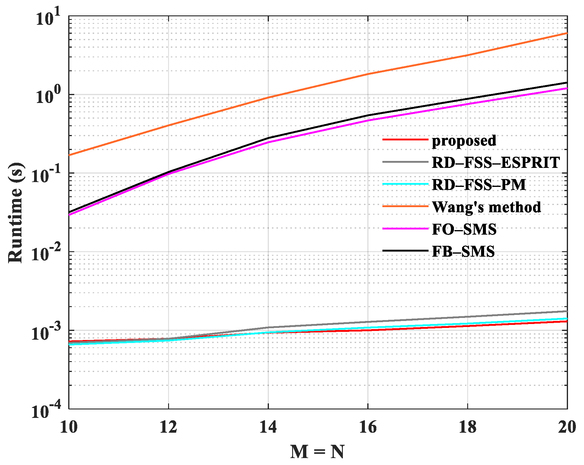
5.4. Runtime Comparison

Finally, we discuss the average runtime to illustrate the computational complexity of each algorithm. It is known from the analysis of the computational complexity that array elements $M$ and $N$ are the main factors that cause the computational time to vary. The simulation is executed on a personal computer with a high-performance Intel i7-9750 H 2.6 GHz processor. We recorded the runtime of each algorithm with MATLAB tools tic and toc. The computational efficiency is equivalently evaluated in terms of CPU time. Assuming that the number of array elements $M=N$ changes and SNR is fixed at 10 dB, there are $K=3$ coherent targets with angles ${\theta }_k=5^{\circ },{10}^{\circ },{15}^{\circ }$ and $f_k=667\mathrm{Hz}$. The number of pulses was $L=150$, and the parameters were $q=10$ and $m^{\prime }=10$ in our proposed algorithm. We also selected appropriate parameters for the rest of the algorithms. The average recording time was taken to obtain the time required for each algorithm to run one Monte Carlo simulation under the corresponding number of array elements. The number of Monte Carlo simulations was 500. Figure 9 depicts the average runtime of these algorithms. Even though RD-FSS-PM can perform the DOA estimation faster, our proposed algorithm requires a very short computation time and the upward trend of the curve is relatively gentle. Moreover, the comparison between the proposed and other algorithms is more obvious with the increase in the number of elements. The average runtime of FB-SMS is slightly longer than that of FO-SMS because more spatial smoothing information must be processed. It can therefore be predicted that the runtime of the proposed algorithm will be very short when the number of array elements is large.

6. Conclusions

In this paper, we have proposed an algorithm for coherent targets in the MIMO radar by considering both the computational burden and estimation accuracy. Our scheme achieves a trade-off between DOA estimation performance and computational complexity. Different from existing approaches, we enlarged the virtual array aperture by exploiting the property of the direction matrix after low-dimensional mapping, and the RCS matrix, which improved the DOF and estimation performance. Moreover, a real-valued approximate signal subspace was achieved by using the unitary Nyström method, which avoids the calculation of the received data covariance matrix and its eigendecomposition. Meanwhile, the real-valued operation had a lower computational complexity than the complex-valued operation. Furthermore, the eigenvector of the approximate signal subspace was used to reconstruct the matrix for direct decorrelation processing. Then, unitary ESPRIT was exploited to estimate the coherent DOAs. The simulation results confirmed the advantages of the proposed method.

References

1. Fishler, E.; Haimovich, A.; Blum, R.; Chizhik, D.; Cimini, L.; Valenzuela, R.A. MIMO Radar: An Idea Whose Time Has Come. In Proceedings of the 2004 IEEE Radar Conference, Philadelphia, PA, USA, 29 April 2004; pp. 71–78. [Google Scholar]
2. Li, J.; Stoica, P.; Xu, L.; Roberts, W. On parameter identifiability of MIMO radar. IEEE Signal Process. Lett. 2007, 14, 968–971. [Google Scholar]
3. Li, J.; Stoica, P. MIMO radar with colocated antennas. IEEE Signal Process. Mag. 2007, 24, 106–114. [Google Scholar] [CrossRef]
4. Haimovich, A.; Blum, R.; Cimini, L. MIMO radar with widely separated antennas. IEEE Signal Process. Mag. 2008, 25, 116–129. [Google Scholar] [CrossRef]
5. Zhai, H.; Meng, X.T.; Yan, F.G. Overview on the target angle estimation technologies for MIMO radar. Radar Sci. Technol. 2021, 19, 144–151. [Google Scholar]
6. Yan, H.D.; Li, J.; Liao, G.S. Multitarget identification and localization using bistatic MIMO radar systems. EURASIP J. Adv. Signal Process. 2007, 2008, 283483. [Google Scholar] [CrossRef] [Green Version]
7. Zhang, X.F.; Xu, L.Y.; Xu, L.; Xu, D.Z. Direction of departure (DOD) and direction of arrival (DOA) estimation in MIMO radar with reduced-dimension MUSIC. IEEE Commun. Lett. 2010, 14, 1161–1163. [Google Scholar] [CrossRef]
8. Jinli, C.; Hong, G.; Weimin, S. Angle estimation using ESPRIT without pairing in MIMO radar. Electron. Lett. 2008, 44, 1422–1423. [Google Scholar] [CrossRef]
9. Duofang, C.; Baixiao, C.; Guodong, Q. Angle estimation using ESPRIT in MIMO radar. Electron. Lett. 2008, 44, 770–771. [Google Scholar] [CrossRef]
10. Qin, G.D.; Bao, D.; Liu, G.G.; Li, P. Cross-correlation matrix Root-MUSIC algorithm for bistatic multiple-input multiple-output radar. Sci. China Inf. Sci. 2015, 58, 1–10. [Google Scholar] [CrossRef] [Green Version]
11. Li, J.F.; Zhang, X.F. Unitary subspace-based method for angle estimation in bistatic MIMO radar. Circuits Syst. Signal Process. 2014, 33, 501–513. [Google Scholar] [CrossRef]
12. Wang, W.; Wang, X.P.; Li, X.; Song, H.R. DOA estimation for monostatic MIMO radar based on unitary root-MUSIC. Int. J. Electron. 2013, 100, 1499–1509. [Google Scholar] [CrossRef]
13. Tang, B.; Tang, J.; Zhang, Y.; Zheng, Z. Maximum likelihood estimation of DOD and DOA for bistatic MIMO radar. Signal Process. 2013, 93, 1349–1357. [Google Scholar] [CrossRef]
14. Liu, B.Y.; Gui, G.; Matsushita, S.Y.; Xu, L. Adaptive filtering algorithm for direction-of-arrival (DOA) estimation with small snapshots. Digit. Signal Process. 2019, 94, 84–95. [Google Scholar] [CrossRef]
15. Chen, H.Y.; Ahmad, F.; Vorobyov, S.; Porikli, F. Tensor decompositions in wireless communications and MIMO radar. IEEE J. Sel. Top. Signal Process. 2021, 15, 438–453. [Google Scholar] [CrossRef]
16. Liu, T.; Wen, F.; Zhang, L.; Wang, K. Off-grid DOA estimation for colocated MIMO radar via reduced-complexity sparse Bayesian learning. IEEE Access 2019, 7, 99907–99916. [Google Scholar] [CrossRef]
17. Zhang, X.F.; Wu, H.L.; Li, J.F.; Xu, D.Z. Computationally efficient DOD and DOA estimation for bistatic MIMO radar with propagator method. Int. J. Electron. 2012, 99, 1207–1221. [Google Scholar] [CrossRef]
18. Shen, C.; Dong, F.; Wen, F.Q.; Gong, Z.H.; Zhang, K. An improved propagator estimator for DOA estimation in monostatic MIMO radar in the presence of imperfect waveforms. IEEE Access 2019, 7, 148771–148778. [Google Scholar] [CrossRef]
19. Gong, J.; Guo, Y.D.; Wan, Q. An improved spatial difference smoothing method based on multistage wiener filtering. Math. Probl. Eng. 2019, 2019, 8515606. [Google Scholar] [CrossRef]
20. Li, J.F.; Jiang, D.F. Performance analysis of propagator-based ESPRIT for direction of arrival estimation. IET Signal Process. 2018, 12, 481–486. [Google Scholar] [CrossRef]
21. Fowlkes, C.; Belongie, S.; Chung, F.; Malik, J. Spectral grouping using the Nystrom method. IEEE Trans. Pattern Anal. Mach. Intell. 2004, 26, 214–225. [Google Scholar] [CrossRef] [Green Version]
22. Qian, C.; Huang, L.; So, H.C. Computationally efficient ESPRIT algorithm for direction-of-arrival estimation based on Nyström method. Signal Process. 2014, 94, 74–80. [Google Scholar] [CrossRef]
23. Veerendra, D. A new approach to achieve a trade-off between direction-of-arrival estimation performance and computational complexity. IEEE Commun. Lett. 2021, 25, 1183–1186. [Google Scholar]
24. Drineas, P.; Mahoney, M.W. On the Nyström method for approximating a Gram matrix for improved kernel-based learning. J. Mach. Learn. Res. 2005, 6, 2153–2175. [Google Scholar]
25. Wang, X.P.; Huang, M.X.; Cao, C.J.; Li, H. Angle estimation noncircular source MIMO radar via unitary Nystrom method. Lect. Notes Electr. Eng. 2019, 463, 339–346. [Google Scholar]
26. Liu, B.B.; Xue, T.; Xu, C.; Liu, Y.J. Computationally efficient unitary ESPRIT algorithm in bistatic MIMO radar. Math. Probl. Eng. 2021, 2021, 5584688. [Google Scholar] [CrossRef]
27. Ye, Z.F.; Luo, D.W.; Wei, J.Q.; Xu, X. Review for coherent DOA estimation technique. J. Data Acquis. Process. 2017, 32, 258–265. [Google Scholar]
28. Pan, J.J.; Sun, M.; Wang, Y.D.; Zhang, X.F. An enhanced spatial smoothing technique with ESPRIT algorithm for direction of arrival estimation in coherent scenarios. IEEE Trans. Signal Process. 2020, 68, 3635–3643. [Google Scholar] [CrossRef]
29. Li, C.C.; Liao, G.S.; Zhu, S.Q.; Wu, S.Y. An ESPRIT-like algorithm for coherent DOA estimation based on data matrix decomposition in MIMO radar. Signal Process. 2011, 91, 1803–1811. [Google Scholar] [CrossRef]
30. Zhang, F.; Jin, A.S.; Hu, Y. Two-dimensional DOA estimation of MIMO radar coherent source based on Toeplitz matrix set reconstruction. Secur. Commun. Netw. 2021, 2021, 6631196. [Google Scholar] [CrossRef]
31. Zheng, Z.D.; Zhang, J.Y.; Wang, T. Coherent angle estimation based on Hankel matrix construction in bistatic MIMO radar. Int. J. Electron. 2013, 100, 190–195. [Google Scholar] [CrossRef]
32. Tabrikian, J.; Bekkerman, I. Transmission Diversity Smoothing for Multi-Target Localization. In Proceedings of the IEEE International Conference on Acoustics, Speech, and Signal Processing, Philadelphia, PA, USA, 23 March 2005; Volume 4, pp. IV-1041–IV-1044. [Google Scholar]
33. Cao, R.Z.; Zhang, X.F. Joint angle and Doppler frequency estimation of coherent targets in monostatic MIMO radar. Int. J. Electron. 2015, 102, 792–814. [Google Scholar] [CrossRef]
34. Cao, R.Z.; Zhang, X.F. Computation efficient joint angle and doppler frequency estimation of coherent targets in monostatic MIMO radar. J. Data Acquis. Process. 2018, 33, 826–836. [Google Scholar]
35. Zhang, W.; Liu, W.; Wang, J.; Wu, S.L. Joint transmission and reception diversity smoothing for direction finding of coherent targets in MIMO radar. IEEE J. Sel. Top. Signal Process. 2014, 8, 115–124. [Google Scholar] [CrossRef] [Green Version]
36. Wang, X.P.; Wang, W.; Ma, Y.H.; Wang, J.X. Joint DOD and DOA estimation for MIMO radar with lower snapshots. J. Harbin Eng. Univ. 2014, 35, 1129–1134. [Google Scholar]
37. Hong, S.; Wan, X.R.; Ke, H.Y. Spatial difference smoothing for coherent sources location in MIMO radar. Signal Process. 2015, 109, 69–83. [Google Scholar] [CrossRef]
38. Shi, J.P.; Hu, G.P.; Zhang, X.F.; Jin, S.S. Smoothing matrix set-based MIMO radar coherent source localization. Int. J. Electron. 2018, 105, 1345–1357. [Google Scholar] [CrossRef]
39. Xenaki, A.; Gerstoft, P.; Mosegaard, K. Compressive beamforming. J. Acoust. Soc. Am. 2014, 136, 260–271. [Google Scholar] [CrossRef] [Green Version]
40. Wen, F.Q.; Zhang, Z.J.; Zhang, G.; Zhang, Y.; Wang, X.H.; Zhang, X.Y. A tensor-based covariance differencing method for direction estimation in bistatic MIMO radar with unknown spatial colored noise. IEEE Access 2017, 5, 18451–18458. [Google Scholar] [CrossRef]
41. Thakre, A.; Haardt, M.; Giridhar, K. Single snapshot spatial smoothing with improved effective array aperture. IEEE Signal Process. Lett. 2009, 16, 505–508. [Google Scholar] [CrossRef]
42. Liu, H.M.; Yang, X.J.; Wang, R.; Jin, W.; Jin, W.M. Transmit/Receive spatial smoothing with improved effective array aperture for angle and mutual coupling estimation in bistatic MIMO Radar. Int. J. Antennas Propag. 2016, 2016, 6271648. [Google Scholar] [CrossRef] [Green Version]
43. Ma, T.; Du, J.; Qiao, L.Y. A Low-Complexity DOA Estimation Algorithm Based on Nyström Method for Mixed Signals. In Proceedings of the 2021 IEEE International Conference on Signal Processing, Communications and Computing (ICSPCC), Xi’an, China, 17–19 August 2021. [Google Scholar]
44. Xu, L.Q.; Li, Y. Low-complexity root-MUSIC algorithm for angle estimation in monostatic MIMO radar. Syst. Eng. Electron. 2017, 39, 2434–2440. [Google Scholar]
Figure 1. The structure of a monostatic MIMO radar.
Remotesensing 14 02646 g001
Figure 2. The distribution of Λ G .
Remotesensing 14 02646 g002
Figure 3. Coherent DOA estimation results over 50 trails in Case 1. (a) SNR = 0 dB; (b) SNR = 20 dB.
Remotesensing 14 02646 g003
Figure 4. Coherent DOA estimation results over 50 trails in Case 2. (a) SNR = 0 dB; (b) SNR = 20 dB.
Remotesensing 14 02646 g004
Figure 5. RMSE versus SNR. (a) Scenario 1: three coherent targets are located at θ k = 5 , 10 , 15 ; (b) Scenario 2: θ k = 45 , 50 , 60 .
Remotesensing 14 02646 g005
Figure 6. RMSE versus snapshots (pulses). (a) Scenario 1: three coherent targets are located at θ k = 10 , 20 , 30 ,   SNR = 10   dB ; (b) Scenario 2: θ k = 45 , 55 , 65 ,   SNR = 20   dB .
Remotesensing 14 02646 g006
Figure 7. RMSE versus the angular separation. (a) Scenario 1: two coherent targets are located at θ k = 10 , 10 + Δ ,   SNR = 0   dB ; (b) Scenario 2: θ k = 60 , 60 + Δ ,   SNR = 0   dB ; (c) Scenario 3: two coherent targets are located at θ k = 10 , 10 + Δ ,   SNR = 20   dB ; (d) Scenario 4: θ k = 60 , 60 + Δ ,   SNR = 20   dB .
Remotesensing 14 02646 g007aRemotesensing 14 02646 g007b
Figure 8. RMSE versus value of m .
Remotesensing 14 02646 g008
Figure 9. Runtime comparison versus array elements M = N .
Remotesensing 14 02646 g009