
Robust Space–Time Joint Sparse Processing Method with Airborne Active Array for Severely Inhomogeneous Clutter Suppression


Abstract
:
1. Introduction
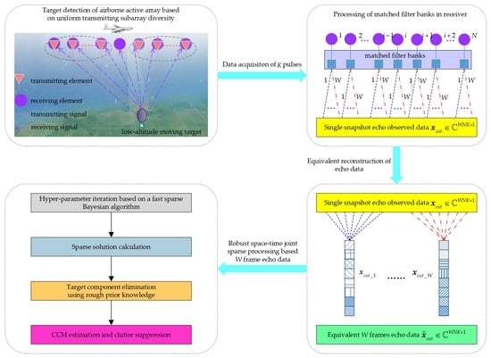
- (1)
- Subarray division on the radar transmitter. The transmitting elements can be divided into several subarrays with the same number of elements in each subarray. In order to realize the spatial diversity of the transmitting subarrays, the orthogonal waveform signals are transmitted among different subarrays. Furthermore, the coherent waveform signal is transmitted within each subarray. In the case of this transmitting form, it can not only acquire the orthogonal transmitting waveform and reduce the dimension of the receiving data, but also utilize the directional gain and the coherence processing gain inside the transmitting subarray. Therefore, greater transmitting domain selectivity is provided for inhomogeneous clutter suppression.
- (2)
- Echo data acquisition of CUT. Multi-group echo data corresponding to different transmitting subarrays can be obtained by a single matched filter bank in each receiving element. Simultaneously, equivalent multi-frame echo data corresponding to all of the transmitting subarrays can be obtained in the whole receiving array.
- (3)
- Sparse spectrum calculation of CUT. Combined with a fast sparse Bayesian learning algorithm, the sparse spectrum of CUT is calculated by the joint sparse processing of the multi-frame echo data.
- (4)
- CCM estimation and clutter suppression. According to the approximate prior information of the target under test, it is removed from the sparse spectrum of CUT. Then, CCM is effectively estimated and the filtering weights are obtained.
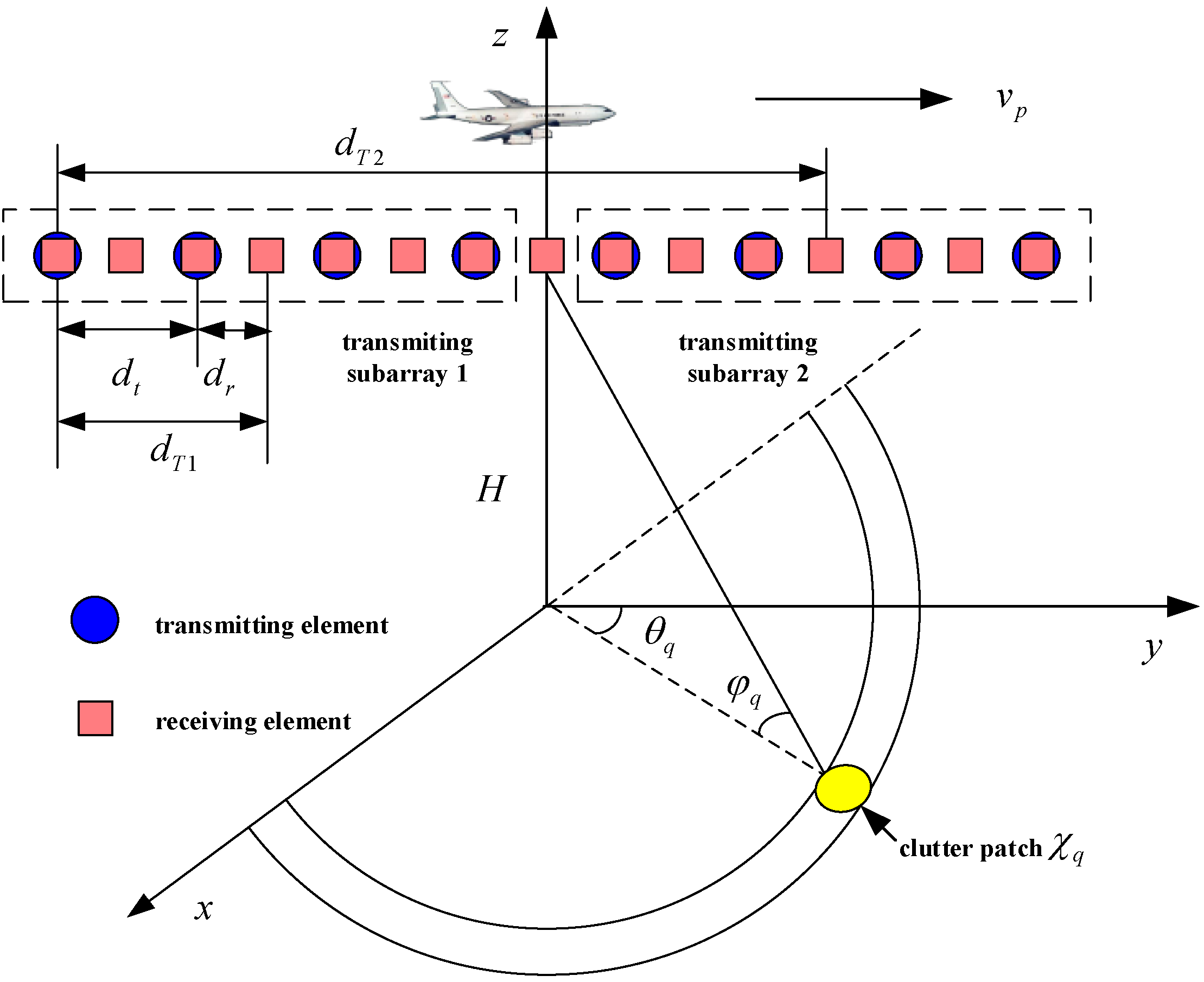
2. Signal Model of Uniform Transmitting Subarray Diversity
3. Space–Time Joint Sparse Processing Based on One Snapshot Echo Observed Data and SBL
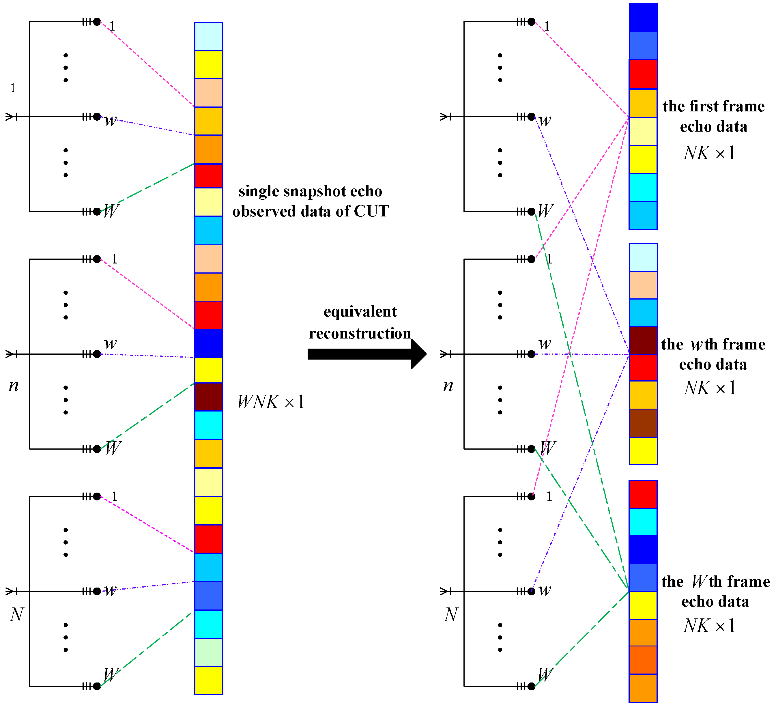
3.1. Equivalent Conversion of the Single Snapshot Echo Observed Data
3.2. Fast Equivalent Multi-Frame Echo Data Joint Sparse Processing Based on SBL
3.2.1. Sparse Solution Calculation of CUT
3.2.2. Clutter Suppression of STAP
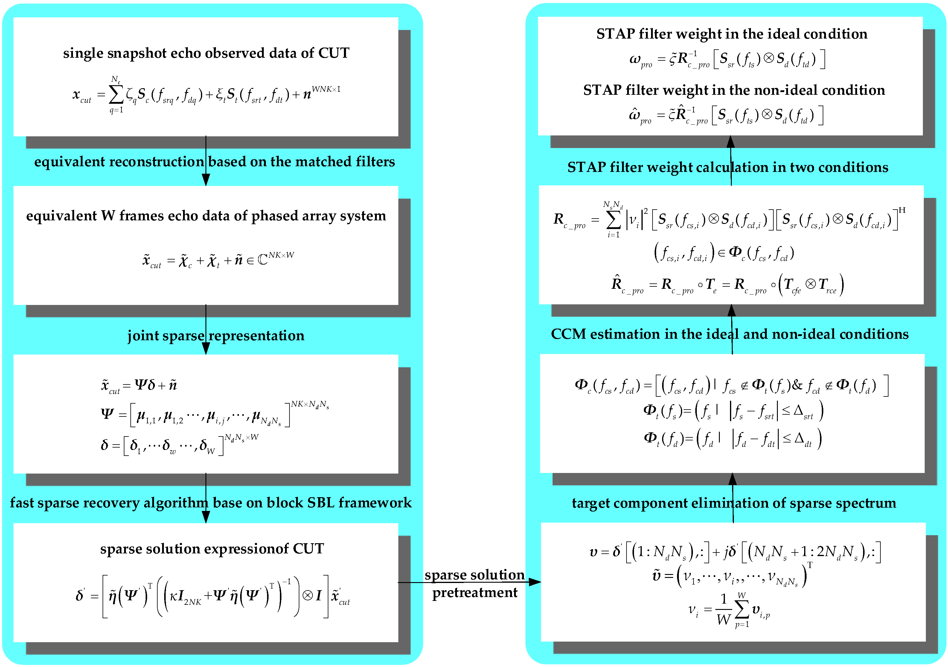
- (1)
- The single snapshot echo observed data of CUT are obtained;
- (2)
- The equivalent W frames’ echo data of the phased array system can be reconstructed;
- (3)
- W frames’ echo data are represented by the joint sparse recovery method;
- (4)
- A fast sparse recovery algorithm based on the block SBL framework is used to obtain the sparse solution expression of the multi-frame echo data of CUT;
- (5)
- The sparse solution should be previously treated so as to adequately utilize the sparse results of W frames’ echo data;
- (6)
- The target components in the sparse solution are eliminated based on the approximate prior knowledge;
- (7)
- CCM can be separately estimated in the ideal and non-ideal conditions;
- (8)
- The filter weight is calculated to realize clutter suppression in the two conditions.
4. Simulation Experiments and Comparative Analyses
4.1. STAP Performance Comparison Using Different Algorithms
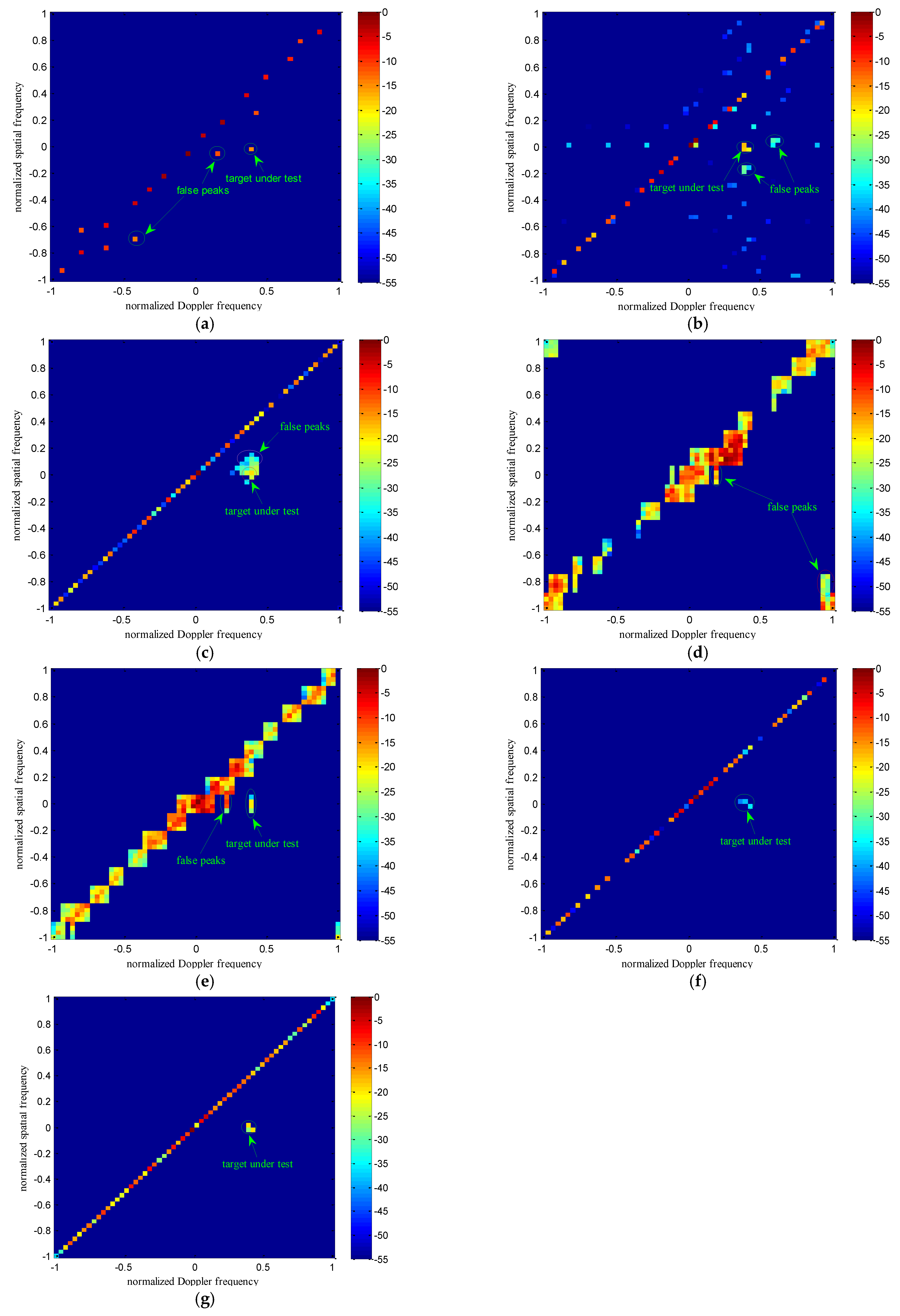
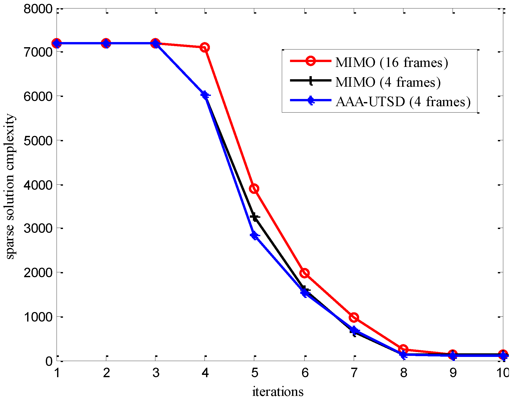
4.1.1. Simulation Results on the Sparse Spectrum
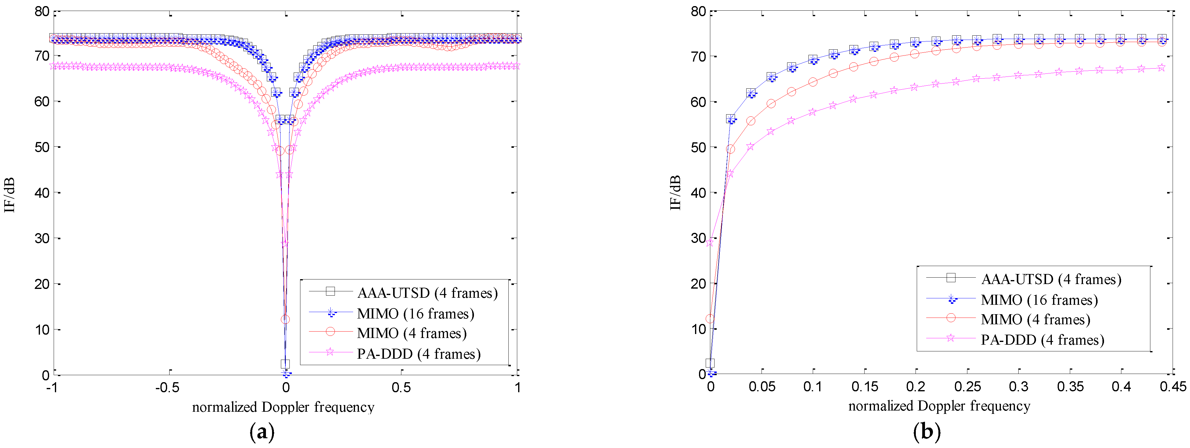
4.1.2. Simulation Results on Improved Factor
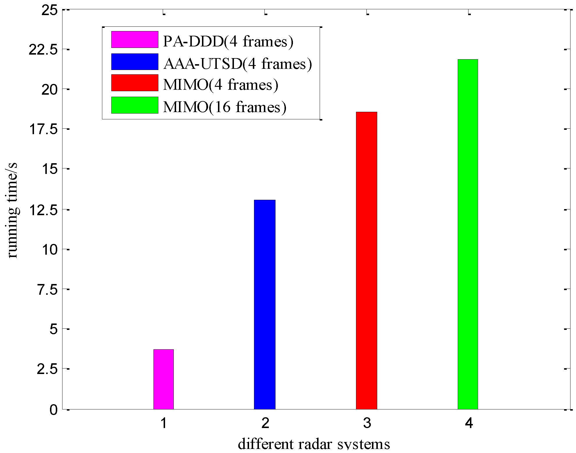
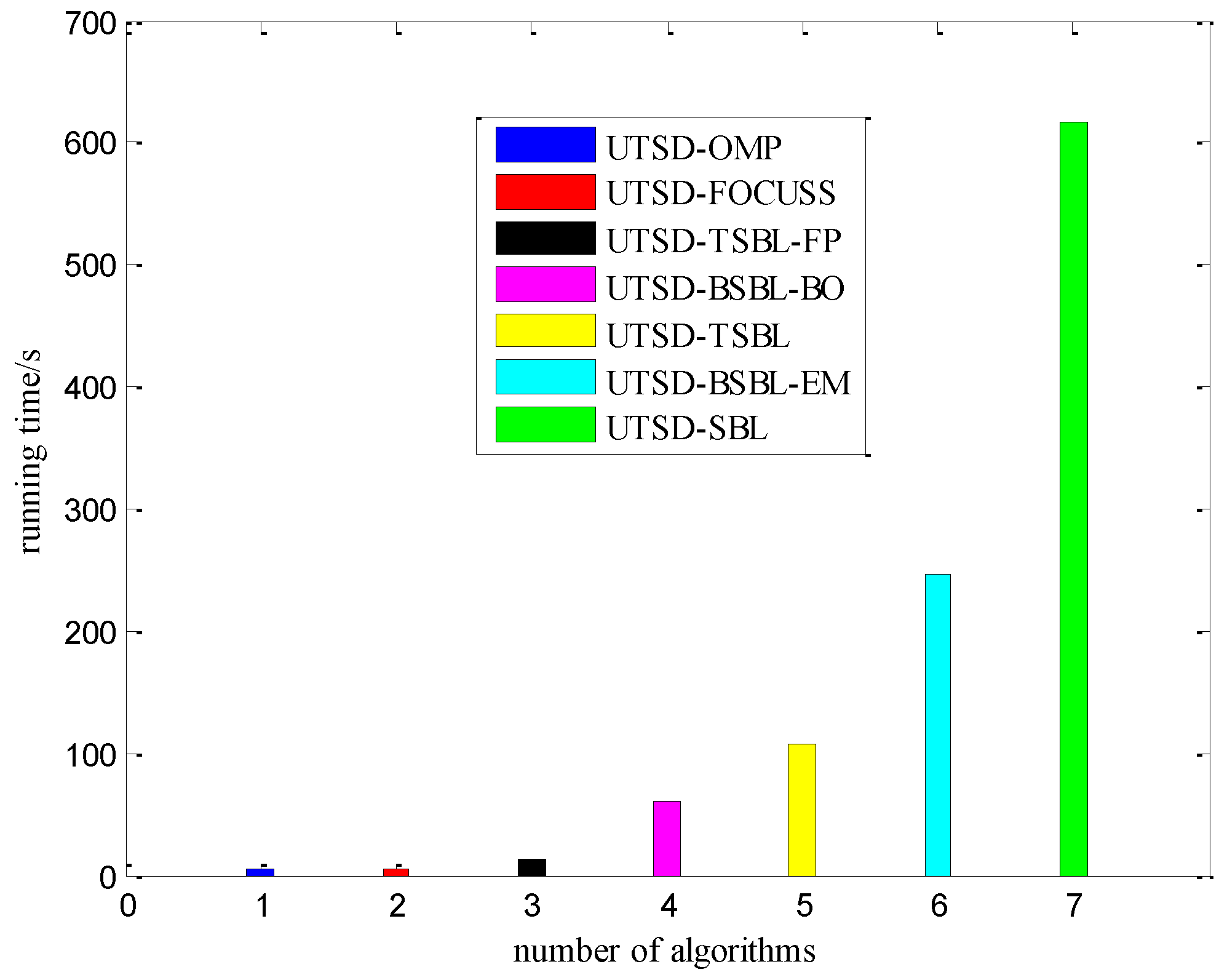
4.1.3. Simulation Results on Running Time
4.2. STAP Performance Comparison Using Different Radar Systems
4.2.1. Simulation Results on Improved Factor
4.2.2. Simulation Results on Running Time
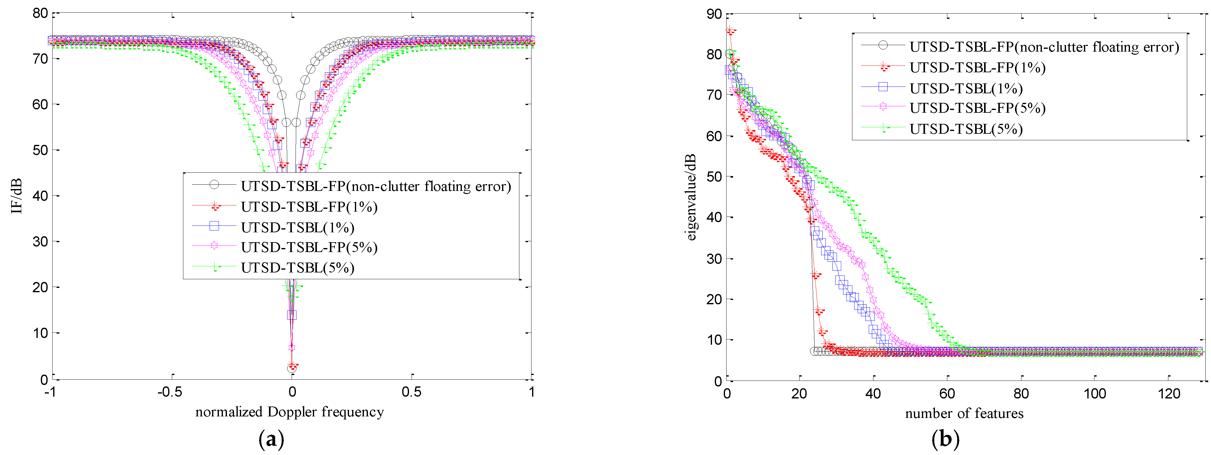
4.3. STAP Performance Comparison in Different Non-Ideal Conditions
5. Conclusions
Author Contributions
Funding
Conflicts of Interest
References
- Barbarossa, S.; Picardi, G. Predictive Adaptive Moving Target Indicator. Signal Process. 1986, 10, 83–97. [Google Scholar] [CrossRef]
- Chen, B.X. Modern Radar System Analysis and Design; Xidian University Press: Xi’an, China, 2012. [Google Scholar]
- Liu, Z.; Ho, D.K.C; Xu, X.Q.; Yang, J.Y. Moving Target Indication Using Deep Convolutional Neural Network. IEEE Access 2018, 6, 65651–65660. [Google Scholar] [CrossRef]
- Wang, Y.L.; Peng, Y.N. Space-Time Adaptive Processing; Tsinghua University Press: Beijing, China, 2000. [Google Scholar]
- Brennan, L.E.; Mallett, J.D.; Reed, I.S. Theory of Adaptive Radar. IEEE Trans. Aerosp. Electron. Syst. 1973, 9, 237–251. [Google Scholar] [CrossRef]
- Jia, F.D.; Sun, G.H.; He, Z.S.; Li, J. Grating-Lobe Clutter Suppression in Uniform Subarray for Airborne Radar STAP. IEEE Sens. J. 2019, 19, 6956–6965. [Google Scholar] [CrossRef]
- Reed, I.S.; Mallett, J.D.; Brennan, L.E. Rapid Convergence Rate in Adaptive Arrays. IEEE Trans. Aerosp. Electron. Syst. 1974, 10, 853–863. [Google Scholar] [CrossRef]
- Shi, J.X; Xie, L.; Cheng, Z.Y.; He, Z.S.; Zhang, W. Angle-Doppler Channel Selection Method for Reduced-Dimension STAP Based on Sequential Convex Programming. IEEE Commun. Lett. 2021, 25, 3080–3084. [Google Scholar] [CrossRef]
- Sui, J.X.; Wang, J.; Zuo, L.; Gao, J. Cascaded Least Square Algorithm for Strong Clutter Removal in Airborne Passive Radar. IEEE Trans. Aerosp. Electron. Syst. 2022, 58, 679–696. [Google Scholar] [CrossRef]
- Chen, N.K.; Wei, P.; Ai, X.Y. A Robust STAP Method Based on Alternating Projection and Clutter Cancellation. IEEE Access 2017, 7, 179880–179890. [Google Scholar] [CrossRef]
- Yang, Z.C.; Wang, X.Y. Reduced-Rank Space-Time Adaptive Processing Algorithm Based on Multistage Selections of Angle-Doppler Filters. IET Radar Sonar Navig. 2022, 16, 327–345. [Google Scholar] [CrossRef]
- Cao, C.H.; Zhang, J.; Meng, J.M.; Zhang, X.; Mao, X.P. Clutter Suppression and Target Tracking by the Low-Rank Representation for Airborne Maritime Surveillance Radar. IEEE Access 2020, 8, 160774–160789. [Google Scholar] [CrossRef]
- Huang, P.H.; Zou, Z.H.; Xia, X.G.; Liu, X.Z.; Liao, G.S. A Novel Dimension-Reduced Space-Time Adaptive Processing Algorithm for Spaceborne Multichannel Surveillance Radar Systems Based on Spatial-Temporal 2-D Sliding Window. IEEE Trans. Geosci. Remote Sens. 2022, 60, 5109721. [Google Scholar] [CrossRef]
- Wang, X.Y.; Yang, Z.C.; Huang, J.J.; Lamare, R.C.D. Robust Two-Stage Reduced-Dimension Sparsity-Aware STAP for Airborne Radar with Coprime Arrays. IEEE Trans. Signal Process. 2020, 68, 81–96. [Google Scholar] [CrossRef]
- Shi, B.; Hao, C.P.; Hou, C.H.; Ma, X.C.; Peng, C.Y. Parametric Rao Test for Multichannel Adaptive Detection of Range-Spread Target in Partially Homogeneous Environments. Signal Process. 2015, 108, 421–429. [Google Scholar] [CrossRef]
- Jiang, C.S.; Li, H.B.; Rangaswamy, M. Conjugate Gradient Parametric Detection of Multichannel Signals. IEEE Trans. Aerosp. Electron. Syst. 2012, 48, 1521–1536. [Google Scholar] [CrossRef]
- Zhao, Y.; Wan, S.H.; Lu, S.T.; Sun, J.P.; Lei, P. Exploiting the Persymmetric Property of Covariance Matrices for Knowledge-Aided Space-Time Adaptive Processing. IEEE Access 2018, 6, 68001–68012. [Google Scholar] [CrossRef]
- Sun, G.H.; He, Z.S.; Tong, J.; Zhang, X.J. Knowledge-Aided Covariance Matrix Estimation via Kronecker Product Expansions for Airborne STAP. IEEE Geosci. Remote Sens. Lett. 2018, 15, 527–531. [Google Scholar] [CrossRef]
- Zhang, W.; He, Z.S.; Li, H.Y. Space Time Adaptive Processing Based on Sparse Recovery and Clutter Reconstructing. IET Radar Sonar Navig. 2019, 13, 789–794. [Google Scholar] [CrossRef]
- Hu, J.F.; Xia, Y.Y.; Li, H.Y.; Liang, J.; Lin, T. A Joint Sparse Space-time Adaptive Processing Method. IEEE Access. 2016, 4, 1–7. [Google Scholar] [CrossRef]
- Liu, M.X.; Zou, L.; Yu, X.L.; Zhou, Y.; Wang, X.G.; Tang, B. Knowledge Aided Covariance Matrix Estimation via Gaussian Kernel Function for Airborne SR-STAP. IEEE Access 2020, 8, 5970–5978. [Google Scholar] [CrossRef]
- Guo, L.; Deng, W.B.; Yao, D.; Yang, Q.; Ye, L.; Zhang, X. A Knowledge-Based on Auxiliary Channel STAP for Target Detection in Shipborne HFSWR. Remote Sens. 2021, 13, 621. [Google Scholar] [CrossRef]
- Liu, K.; Wang, T.; Wu, J.X.; Chen, J.M. A Two-Stage STAP Method Based on Fine Doppler Localization and Sparse Bayesian Learning in the Presence of Arbitrary Array Errors. Sensors 2022, 22, 77. [Google Scholar] [CrossRef] [PubMed]
- Cui, N.; Xing, K.; Duan, K.Q.; Yu, Z.J. Knowledge-Aided Block Sparse Bayesian Learning STAP for Phased-Array MIMO Airborne Radar. IET Radar Sonar Navig. 2021, 15, 1628–1642. [Google Scholar] [CrossRef]
- Cristallini, D.; Bürger, W. A Robust Direct Data Domain Approach for STAP. IEEE Trans. Signal Process. 2012, 60, 1283–1294. [Google Scholar] [CrossRef]
- Yang, Z.C.; Fa, R.; Qin, Y.L.; Li, X.; Wang, H.Q. Direct Data Domain Sparsity-Based STAP Utilizing Subaperture Smoothing Techniques. Int. J. Antenna Propag. 2015, 2015, 171808. [Google Scholar] [CrossRef] [Green Version]
- Li, M.; Sun, G.H.; He, Z.S. Direct Data Domain STAP Based on Atomic Norm Minimization. In Proceedings of the 2019 IEEE Radar Conference, Boston, MA, USA, 22–26 April 2019; pp. 1–6. [Google Scholar]
- Gao, Z.Q.; Tao, H.H. Knowledge-Aided Direct Data Domain STAP Algorithm for Forward-looking Airborne Radar. In Proceedings of the 2019 IEEE International Conference on Signal, Information and Data Processing (ICSIDP), Chongqing, China, 11–13 December 2019; pp. 1–6. [Google Scholar]
- Xiao, H.; Wang, T.; Wen, C.; Ren, B. A Generalized Eigenvalue Reweighting Covariance Matrix Estimation Algorithm for Airborne STAP Radar in Complex Environment. IET Radar Sonar Navig. 2021, 15, 1309–1324. [Google Scholar] [CrossRef]
- Bil, R.; Holpp, W. Modern Phased Array Radar Systems in Germany. In Proceedings of the 2016 IEEE International Symposium on Phased Array Systems and Technology (PAST), Waltham, MA, USA, 18–21 October 2016; pp. 1–7. [Google Scholar]
- Alkhafaji, N.; Campbell, R.L.; Roche, M. Microwave Modulated Scatter Active Array Distortion Sidelobes. IEEE Trans. Microw. Theory Tech. 2020, 68, 328–338. [Google Scholar] [CrossRef]
- Kinghorn, T.; Scott, I.; Totten, E. Recent Advances in Airborne Phased Array Radar Systems. In Proceedings of the 2016 IEEE International Symposium on Phased Array Systems and Technology (PAST), Waltham, MA, USA, 18–21 October 2016; pp. 1–7. [Google Scholar]
- Burger, W.K. Sidelobe Forming for Ground Clutter and Jammer Suppression for Airborne Active Array Radar. In Proceedings of the IEEE International Symposium on Phased Array Systems and Technology, Boston, MA, USA, 14–17 October 2003; pp. 271–276. [Google Scholar]
- Rose, P.S.; Finlay, C.D. Reducing Clutter in Airborne Radars Equipped with Active Electronically Steered Array Antennas by Using a Novel Receive Aperture Weighting. In Proceedings of the 2008 IEEE Radar Conference, Rome, Italy, 26–30 May 2008; pp. 573–577. [Google Scholar]
- Wijenayake, C.; Madanayake, A.; Belostotski, L.; Xu, Y.; Bruton, L. All-Pass Filter-Based 2-D IIR Filter-Enhanced Beamformers for AESA Receivers. IEEE Trans. Circuits Syst. I-Regul. Pap. 2014, 61, 1331–1342. [Google Scholar] [CrossRef]
- Buerger, W.; Perna, I. Knowledge Aided STAP/GMTI with Subarrayed AESA Radar. In Proceedings of the EUSAR 2016: 11th European Conference on Synthetic Aperture Radar (EUSAR), Hamburg, Germany, 7–9 June 2016; pp. 220–225. [Google Scholar]
- Zhang, X.C.; Xie, W.C.; Zhang, Y.S.; Wang, Y.L. Modeling and Analysis of the Clutter on Airborne MIMO Radar with Arbitrary Waveform Correlation. J. Electron. Inf. Technol. 2011, 33, 646–651. [Google Scholar] [CrossRef]
- Zhang, X.C.; Zhang, Y.S.; Xie, W.C.; Wang, Y.L. Research on the Estimation of Clutter Rank for Coherent Airborne MIMO Radar. J. Electron. Inf. Technol. 2011, 33, 2125–2131. [Google Scholar] [CrossRef]
- Feng, W.K.; Zhang, Y.S. MMV-JSR Based STAP Method Using MIMO Radar. IEICE Comm. Express. 2016, 5, 163–168. [Google Scholar] [CrossRef] [Green Version]
- Gan, F.P.; Wang, H.B.; Fang, Y.; Zhang, K.; Qin, G.-J.; Zhao, X. Reconstruction of Heart Sound Based on CS and BSBL. Comput. Eng. Des. 2016, 37, 1037–1041. [Google Scholar]
- Jiang, K.; Wang, H.F.; Shahidehpour, M.; He, B.T. Block-Sparse Bayesian Learning Method for Fault Location in Active Distribution Networks with Limited Synchronized Measurements. IEEE Trans. Power Syst. 2021, 36, 3189–3203. [Google Scholar] [CrossRef]
- Zhang, Z.L.; Rao, B.D. Sparse Signal Recovery with Temporally Correlated Source Vectors Using Sparse Bayesian Learning. IEEE J. Sel. Top. Signal Process. 2011, 5, 912–926. [Google Scholar] [CrossRef] [Green Version]
- Song, Q.J. Research on Sparse Bayesian Learning Base Sparse Channel Estimation in Underwater Acoustic OFDM Communication. Ph.D. Thesis, Harbin Engineering University, Harbin, China, 2020. [Google Scholar]
- Qiao, G.; Song, Q.J.; Ma, L.; Liu, S.Z.; Sun, Z.; Gan, S. Sparse Bayesian Learning for Channel Estimation in Time-Varying Underwater Acoustic OFDM Communication. IEEE Access 2018, 6, 56675–56684. [Google Scholar] [CrossRef]
- Zhang, Z.L.; Rao, B.D. Recovery of Block Sparse Signals Using the Framework of Block Sparse Bayesian Learning. In Proceedings of the 2012 IEEE International Conference on Acoustics, Speech and Signal Processing (ICASSP), Kyoto, Japan, 25–30 March 2012; pp. 3345–3348. [Google Scholar]
- MacKay, D.J.C. Bayesian Interpolation. Neural Comput. 1992, 4, 131–134. [Google Scholar] [CrossRef]
- Tropp, J.A.; Gilbert, A.C. Signal Recovery from Random Measurements via Orthogonal Matching Pursuit. IEEE Trans. Info. Theory 2007, 53, 4655–4666. [Google Scholar] [CrossRef] [Green Version]
- Gorodnitsky, I.F.; Rao, B.D. Sparse Signal Reconstruction from Limited Data Using FOCUSS: A Re-Weighted Minimum Norm Algorithm. IEEE Trans. Signal Process. 1997, 45, 600–616. [Google Scholar] [CrossRef] [Green Version]
- Balkan, O.; Kreutz-Delgado, K.; Makeig, S. Localization of More Sources than Sensors via Jointly Sparse Bayesian Learning. IEEE Signal Process. 2014, 21, 131–134. [Google Scholar] [CrossRef]
- Shi, J.P.; Yang, Z.; Liu, Y.X. On Parameter Identifiability of Diversity-Smoothing-Based MIMO Radar. IEEE Trans. Aerosp. Electron. Syst. 2021, in press. [CrossRef]
- Wang, X.P.; Yang, L.T.; Dong, M.X.; Ota, K.; Wang, H.F. Multi-UAV Cooperative Localization for Marine Targets Based on Weighted Subspace Fitting in SAGIN Environment. IEEE Internet Things J. 2022, 9, 5708–5718. [Google Scholar] [CrossRef]


| Parameter | Value | Parameter | Value |
|---|---|---|---|
| transmitting element size | 16 | number of coherent pulses | 8 |
| receiving element size | 16 | airborne velocity (m/s) | 140 |
| radar wavelength (m) | 0.23 | airborne height (m) | 8000 |
| number of transmitting subarrays | 4 | target velocity (m/s) | 28 |
| number of elements in each subarray | 4 | signal-to-noise ratio (dB) | 20 |
| transmitting element interval (m) | 0.115 | clutter-to-noise ratio (dB) | 60 |
| receiving element interval (m) | 0.115 | normalized temporal frequency | 0.4 |
| pulse repetition frequency (Hz) | 2434.8 | normalized spatial frequency | 0 |
Publisher’s Note: MDPI stays neutral with regard to jurisdictional claims in published maps and institutional affiliations. |
© 2022 by the authors. Licensee MDPI, Basel, Switzerland. This article is an open access article distributed under the terms and conditions of the Creative Commons Attribution (CC BY) license (https://creativecommons.org/licenses/by/4.0/).
Share and Cite
Wang, Q.; Xue, B.; Hu, X.; Wu, G.; Zhao, W. Robust Space–Time Joint Sparse Processing Method with Airborne Active Array for Severely Inhomogeneous Clutter Suppression. Remote Sens. 2022, 14, 2647. https://doi.org/10.3390/rs14112647
Wang Q, Xue B, Hu X, Wu G, Zhao W. Robust Space–Time Joint Sparse Processing Method with Airborne Active Array for Severely Inhomogeneous Clutter Suppression. Remote Sensing. 2022; 14(11):2647. https://doi.org/10.3390/rs14112647
Chicago/Turabian StyleWang, Qiang, Bin Xue, Xiaowei Hu, Guangen Wu, and Weihu Zhao. 2022. "Robust Space–Time Joint Sparse Processing Method with Airborne Active Array for Severely Inhomogeneous Clutter Suppression" Remote Sensing 14, no. 11: 2647. https://doi.org/10.3390/rs14112647
APA StyleWang, Q., Xue, B., Hu, X., Wu, G., & Zhao, W. (2022). Robust Space–Time Joint Sparse Processing Method with Airborne Active Array for Severely Inhomogeneous Clutter Suppression. Remote Sensing, 14(11), 2647. https://doi.org/10.3390/rs14112647