Article

Remote Sensing Phenology of the Brazilian Caatinga and Its Environmental Drivers

by
Rodolpho Medeiros
1,
João Andrade
2,
Desirée Ramos
3,
Magna Moura
4,
Aldrin Martin Pérez-Marin
5,
Carlos A. C. dos Santos
1,
Bernardo Barbosa da Silva
1 and
John Cunha
6,*
1
Academic Unity of Atmospheric Sciences, Technology and Natural Resources Center, Federal University of Campina Grande, Campina Grande 58109-970, Brazil
2
Centre for Technology and Geosciences, Department of Civil Engineering, Federal University of Pernambuco, Recife 50740-550, Brazil
3
Phenology Lab, Department of Botany, Institute of Biosciences, São Paulo State University (UNESP), Rio Claro, SP 14884-900, Brazil
4
Empresa Brasileira de Pesquisa Agropecuária, Embrapa Semiárido, Petrolina 56302-970, Brazil
5
National Institute of Semi-Arid, Campina Grande 58429-970, Brazil
6
Centre for the Sustainable Development of the Semi-Arid, Federal University of Campina Grande, Campina Grande 58429-900, Brazil
*
Author to whom correspondence should be addressed.
Remote Sens. 2022, 14(11), 2637; https://doi.org/10.3390/rs14112637
Submission received: 30 April 2022 / Revised: 30 May 2022 / Accepted: 30 May 2022 / Published: 31 May 2022
(This article belongs to the Special Issue Remote Sensing of Land Surface Phenology)

Abstract

:
The Caatinga is the largest nucleus of Seasonally Dry Tropical Forests (SDTF) in the Neotropics. The leafing patterns of SDTF vegetation are adapted to the current environmental and climate variability, but the impacts of climate change tend to alter plants’ phenology. Thus, it is necessary to characterise phenological parameters and evaluate the relationship between vegetation and environmental drivers. From this information, it is possible to identify the dominant forces in the environment that trigger the phenological dynamics of the Caatinga. In this way, remote sensing represents an essential tool to investigate the phenology of vegetation, particularly as it has a long series of vegetation monitoring and allows relationships with different environmental drivers. This study has two objectives: (i) estimate phenological parameters using an Enhanced Vegetation Index (EVI) time-series over 20 years, and (ii) characterise the relationship between phenologic dynamics and environmental drivers. TIMESAT software was used to determine four phenological parameters: Start Of Season (SOS), End Of Season (EOS), Length Of Season (LOS), and Amplitude (AMPL). Boxplots, Pearson’s, and partial correlation coefficients defined relationships between phenologic dynamics and environmental drivers. The non-parametric test of Fligner–Killeen was used to test the interannual variability in SOS and EOS. Our results show that the seasonality of vegetation growth in the Caatinga was different in the three experimental sites. The SOS was the parameter that presented the greatest variability in the days of the year (DOY), reaching a variation of 117 days. The sites with the highest SOS variability are the same ones that showed the lowest EOS variation. In addition, the values of LOS and AMPL are directly linked to the annual distribution of rainfall, and the longer the rainy season, the greater their values are. The variability of the natural cycles of the environmental drivers that regulate the ecosystem’s phenology and the influence on the Caatinga’s natural dynamics indicated a greater sensitivity of the phenologic dynamics to water availability, with precipitation being the limiting factor of the phenologic dynamics. Highlights: The EVI time series was efficient in estimating phenological parameters. The high variability of the start of season (SOS) occurred in sites with low variability of end of the season (EOS) and vice versa. The precipitation and water deficit presented a higher correlation coefficient with phenological dynamics. Length of Season (LOS) and amplitude (AMPL) are directly linked to the annual distribution of rainfall.

1. Introduction

The Seasonally Dry Tropical Forests (SDTF) are characterised by a strong seasonal and irregular distribution of rainfall throughout the year, resulting in long dry season periods [1,2]. The Brazilian Caatinga, with an area of approximately 900,000 km2, is the largest nucleus of SDTF in the Neotropics [The tropical New World biogeographic region comprises Central America, the Caribbean, and South America] [3]. Moreover, with 3347 plant species, of which 526 are endemic, the Caatinga is the richest nucleus of SDTF in the Neotropics [4]. Its remarkable floristic diversity makes the Caatinga twice as rich as the Amazon rainforest when considering the species/area relationship [4]. Phenology studies recurring life-cycle events such as bird migration, flower blooming, or leaf emergence and senescence and the causes of their timing by biotic and abiotic forces [5,6]. The leafing patterns of Caatinga vegetation are adapted to the intense climate and water seasonality, being highly dependent on the climate interannual variability [7,8]. Most leaves fall during the dry season, and the first rainfall pulses trigger a quick leaf flush in the wet season [7,8,9].
Precipitation and soil moisture are the leading environmental drivers for the leaf changes in the Caatinga [8,9]. Still, the temperature can also be a driver for species presenting scheduled phenology in dry ecosystems [10]. The Intergovernmental Panel on Climate Change [11] forecasts an increase of 1.5 °C in the global mean air temperature for the next two decades in an optimistic scenario, considering the reduction of current emissions of CO2. Besides the temperature increases, climate changes are likely to alter the precipitation regimes in the following decades [12,13]. The consequences of these changes are, among others, the projected drying out of surface soils [12] and prolonged dry seasons, with an increase of 47% of the area of the Northeast Region of Brazil (NEB) subjected to extreme drought events until 2070 [13]. Thus, understanding the past and current vegetation’s response to the environmental drivers is paramount to predicting its behaviour in climate change scenarios, allowing the detection of changes in the timing of leaf patterns and their causes.
The ability to monitor global vegetation phenology, or Land Surface Phenology (LSP), has increased with the validated Remote Sensing (RS) and modelling approaches to mapping phenology [14,15]. Long-term data from satellite products are useful tools for understanding the phenological responses of vegetation to current environmental drivers using Vegetation Indices (VIs), allowing it to predict its responses to climate change scenarios. VIs time series has received the attention given its potential to characterise interactions between climate and vegetation with broad applications in different ecosystems [16,17,18]. Several VIs are calculated based upon different spectral bands and, therefore, evidence of different components of the environment [19]. The Enhanced Vegetation Index (EVI) has been widely used to characterise vegetation phenology [20,21] due to its sensitivity to high biomass and reduced atmospheric and soil effects. EVI is calculated from the near-infrared (NIR), Red, and Blue bands and can be derived for different satellite platforms, such as Landsat, Sentinel, and MODIS. The use of algorithms to determine the main phenological metrics from the VIs time series has favoured the representation of the phenological stages of each cropping system, allowing a crop-type classification based on their phenological metrics [22]. However, the studies driving this on a global scale have been primarily focused on forest ecosystems, associating phenological changes in vegetation with climate patterns, particularly with rainfall data [23]. These studies showed that the phenological dynamics strongly depend on the seasonality of rainfall [21,24]. Still, the studies on a regional scale indicate that other environmental drivers also trigger phenological changes [25,26,27,28].
The LSP applied to an ecosystem scale seems to offer the best opportunities to advance understanding of environmental triggers and determinants for phenological dynamics, given the possibility to understand it on a broad scale, encompassing areas in a range of contrasting environmental conditions. For instance, the early greening or pre-rain green-up, a phenomenon where trees produce leaves before the rain starts, was registered in the woodlands and savannas of southern Africa through RS satellite techniques [29,30]. Furthermore, the application of the LSP at a continental scale and using long-term time-series (2002–2014) allowed us to measure the variability in leaf flushing (i.e., greening) among years and to identify the photoperiod as the environmental cue for early greening [30].
The use of LSP and their drivers will be significant for SDTFs where interannual rainfall variability and rainy season duration change on a spatial and temporal scale [31,32], factors that are expected to influence the phenological strategies of plant communities in this vegetation [10]. There was also great regional variability and interannual fluctuation in vegetation phenology, and the overall phenological trends shifted later [21]. By following the studies for dry forests, Tong et al. [15] reported that the interannual rainfall variability was a more dominant force than fire events and land-use change in the phenological trend in tropical areas. For example, Jesus et al. [25] noticed changes in the phenological patterns for dense and open vegetation areas of the Caatinga, suggesting that factors that vary at spatial scales, such as the vegetation structure, would also be necessary for the phenological responses of the vegetation. In an experimental area in the Caatinga, the phenological response was directly related to soil water availability [9].
Despite advances in the analysis of phenological patterns and their associated environmental drivers, mainly observed in studies at the ecosystem scale, the application of long-term time series of vegetation indices in studies of the Caatinga vegetation is scarce. In addition, there are limitations to the diversity of sites studied for the Caatinga. For example, when analysing the dominant environmental drivers for the phenology of seasonally dry ecosystems (Caatinga, Cerrado), Alberton et al. [33] observed that the dominant drivers in these ecosystems were distinct, with light (measured as day-length) being more relevant in explaining leafing patterns in Cerrado communities than rainfall for Caatinga communities. Therefore, comparing sites of the same ecosystem can better define the environmental drivers associated with the phenological dynamics. There are also limitations to the number of environmental drivers analysed in the studies carried out for the Caatinga. Analysis with more environmental drivers could reveal meaningful soil–plant–atmosphere interactions, which may occur to a lesser extent.
Given the above, this study proposes to evaluate the Caatinga phenological sensitivity to environmental drivers in three Caatinga ecoregions. The seasonality of vegetation will be observed from the EVI time series over 20 years (2000–2019) and environmental drivers (precipitation, air temperature, soil moisture, and water deficit) from global databases. This study has two objectives: (i) estimate phenological parameters using an EVI time-series over 20 years, and (ii) characterise the relationship between phenologic dynamics and environmental drivers. The results will also be expected to serve as a baseline against which to compare future changes in Caatinga phenology due to natural or anthropogenic causes.

2. Material and Methods
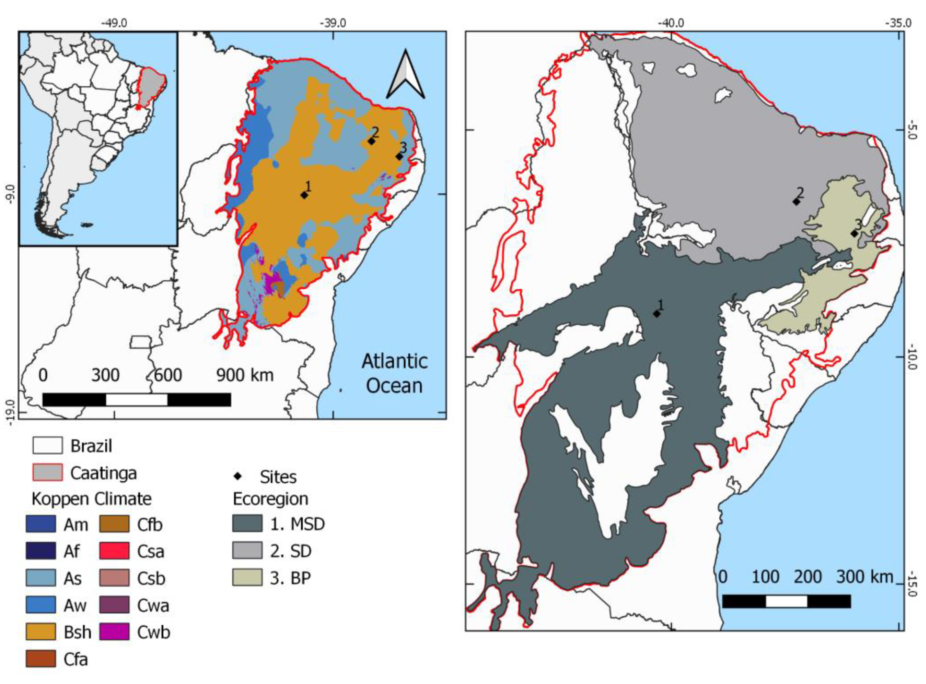
2.1. Study Areas

The semi-arid climate (Köppen’s BSh) [34], where the Caatinga is located, presents accumulated precipitation below 600 mm and an average air temperature of 25 °C to 30 °C throughout the year [35]. However, seasonally, the average annual rainfall varies widely from 300 mm to 1000 mm annually, mainly concentrated in a period of 3 to 4 months, during summer and autumn, followed by a prolonged dry season lasting 8 to 9 months during winter and spring [36]. The Caatinga is characterised by high interannual precipitation variability, with droughts that can last for years and high potential evapotranspiration rates of between 1500 mm and 2000 mm annually [37]. The Caatinga region has different soil categories, ranging from shallow, rocky, and relatively fertile to deep with high natural fertility and sedimentary or sandy, deep, and non-fertile [35]. In the Caatinga, the typical vegetation comprises deciduous and thorny forests or small forests that grow mainly in exposed crystalline rocky terrains, such as the Depression Sertaneja [38]. The region’s geomorphology ranges from lowlands of 300 m, mountains, plateaus, and plateaus with an altitude of up to 1000 m [35].
The study was carried out at three SDTF protected sites, each area being in a different ecoregion (Figure 1): (i) Meridional Sertaneja Depression (MSD) ecoregion experimental site located Embrapa Semi-arid, Petrolina, Pernambuco; (ii) Sertanejas Depressions (SD) ecoregion experimental site located at Seridó Ecological Station, Serra Negra do Norte, Paraíba; (iii) Borborema Plateau (BP) ecoregion experimental site located at Semi-arid National Institute, Campina Grande, Paraíba. The MSD experimental site’s geographic coordinates are 9°02′47″ S, 40°19′16″ W, 395 m altitude, and its vegetation is dry xerophilous forest, with trees and shrubs that average five metres in height [39]. The average annual temperature is 26.2 °C, and the rainfall is 387 mm [39], concentrated mainly from January to April. The predominant soil type in the experimental site is Red-Yellow Argisol, followed by Haplossol and Hydromorphic Vertisol [40]. The SD experimental site’s geographic coordinates are 6°34′42″ S, 37°15′05″ W, and 203 m altitude. Its area is characterised by dry xerophilous forest with deciduous plant species and the predominance of small, widely dispersed trees and shrubs up to 10 metres high, which develop and grow only in the rainy season between January and May [41]. The average annual precipitation varies between 400 and 700 mm, and the average yearly temperature ranges from 28 to 30 °C. The dominant soil is Neosol Litolic, shallow (about 40 cm), stony, and low fertility [42]. The BP experimental site’s geographic coordinates are 7°16′49″ S, 35°58′34″ W, and 492 m altitude. The vegetation present in the experimental site is composed of dense Caatinga, with tree heights between three and seven metres. The region experiences a rainy season starting in March/April and extending until August, while the dry season lasts for five to six months [43]. The average annual rainfall of Campina Grande is about 750 mm, and the average annual air temperature is 23.3 °C [44]. The soil is nitric planosol [45].

2.2. Data Processing

The processes for obtaining geospatial images and data were performed using the Google Earth Engine (GEE) tool [46]. Cloud computing platforms, such as GEE, facilitate the processing of satellite images globally. With access and analysis of several petabytes of images and a broad set of geospatial data, dating from 40 years of Earth observation data, updated and expanded daily, the tool allows viewing, manipulating, editing, and creating spatial data [46]. The EVI vegetation indices derived from the Moderate Resolution Imaging Spectroradiometer (MODIS) sensor reflectance data were used to represent the variability of native vegetation, investigating some biophysical mechanisms that involve soil–plant–atmosphere relationships in the natural dynamics of the Caatinga. The MODIS sensor images and the TerraClimate and CHIRPS data sets’ environmental drivers were evaluated from 2000 to 2019. The environmental drivers were made up of monthly precipitation, air temperature, soil moisture, and water deficit time series for the three experimental areas.

2.2.1. MODIS Data

This research used the surface reflectance data of the MODIS 16-day nadir BRDF-Adjusted Reflectance product (MCD43A4); the dataset is produced daily using 16 days of Terra and Aqua MODIS data at 500 metres resolution. The reflectance bands were used to obtain the EVI vegetation index [47]. The first available images of MODIS date from February 2000, and this study had its period limited to including images until December 2019. The EVI series were assembled for each studied site, with the value of the MCD43A4 product pixel corresponding to the geographic coordinates of each testing location. After that, the EVI time series was converted into a monthly EVI time series, using the mean value of each month.

2.2.2. TerraClimate e CHIRPS Data

The air temperature, precipitation, soil moisture, and water deficit are some of the potential environmental drivers for the leaf exchange strategies of Caatinga plant species [33]. These possible environmental drivers acting on the Caatinga vegetation were observed in three different sites of the Caatinga. All the variables mentioned were obtained monthly from the TerraClimate data set [48], except for precipitation data. Monthly precipitation data were obtained from the Climate Hazards Group InfraRed Precipitation with Stations (CHIRPS) database [49]. The exact centre pixels used to construct the EVI time series were used to obtain the environmental drivers’ time series.

2.2.3. Phenological Metrics

The phenological metrics represent the characteristics of the vegetation within its phenological cycle, or phenophases, corresponding to dimensionless output parameters and can be calculated based on the EVI time series. In this study, the TIMESAT software [50,51] was used to analyse 20 years of EVI time series (from 2000 to 2019) and to compute 4 phenological metrics: Start of Season (SOS), End Of Season (EOS), Length of the season (LOS), and Amplitude (AMPL) difference between the peak and the base level value. After applying the Savitzky-Golay filter [52] in TIMESAT, a seasonality parameter per year was chosen, representing a phenological cycle with a start and end level of 20% of the seasonal amplitude. This threshold value was used in several studies and is known to be accurate in registering the plant’s phenological transitions [53,54,55,56,57,58]. The four phenological metrics are shown in boxplot graphics for each ecoregion studied and used for correlations with environmental drivers.

2.2.4. Seasonal Variability Analysis

Interannual variability in phenological metrics across sites—To test if the interannual variability in SOS and EOS (i.e., the variances in phenological transition dates) differs among the three sites, we used the non-parametric test Fligner–Killeen [59]. The Fligner–Killeen test compares the homogeneity of variances among samples [59]. The same analysis was performed to test if the variability of SOS differs from the EOS within each site. To test if the LOS and the AMPL of EVI differ among sites, we performed a one-way analysis of variance (ANOVA) followed by the Tukey post-hoc test. In addition, we used box plots to compare the three experimental sites’ seasonal data on EVI, phenological metrics, and environmental drivers for 20 years.
Influence of environmental drivers on phenological metrics—The environmental drivers were also observed monthly to assess their influence on phenological parameters. This study analysed these relationships through scatter plots with smoothed (r) correlation curves from Pearson’s classification (P) between the EVI and environmental drivers. Pearson’s correlation between EVI time series and monthly environmental drivers was submitted to different monthly lag periods (0–3). The lag monthly of each environmental driver with the highest Pearson’s correlation was applied to the partial correlation method. Then the partial correlation method was used to analyse the environmental drivers in the monthly EVI time series [60]. Data analysis was carried out in R [61].

3. Results

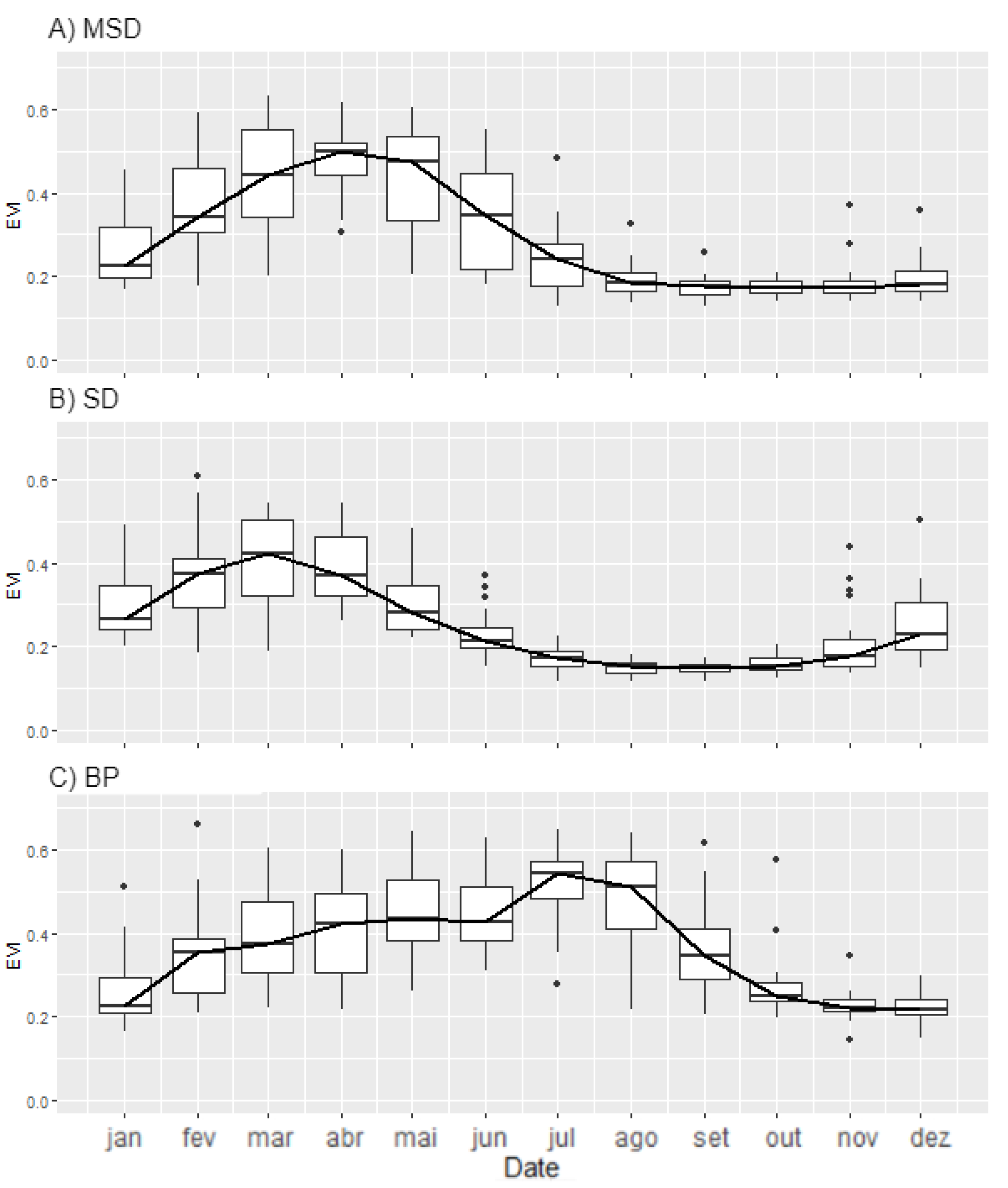
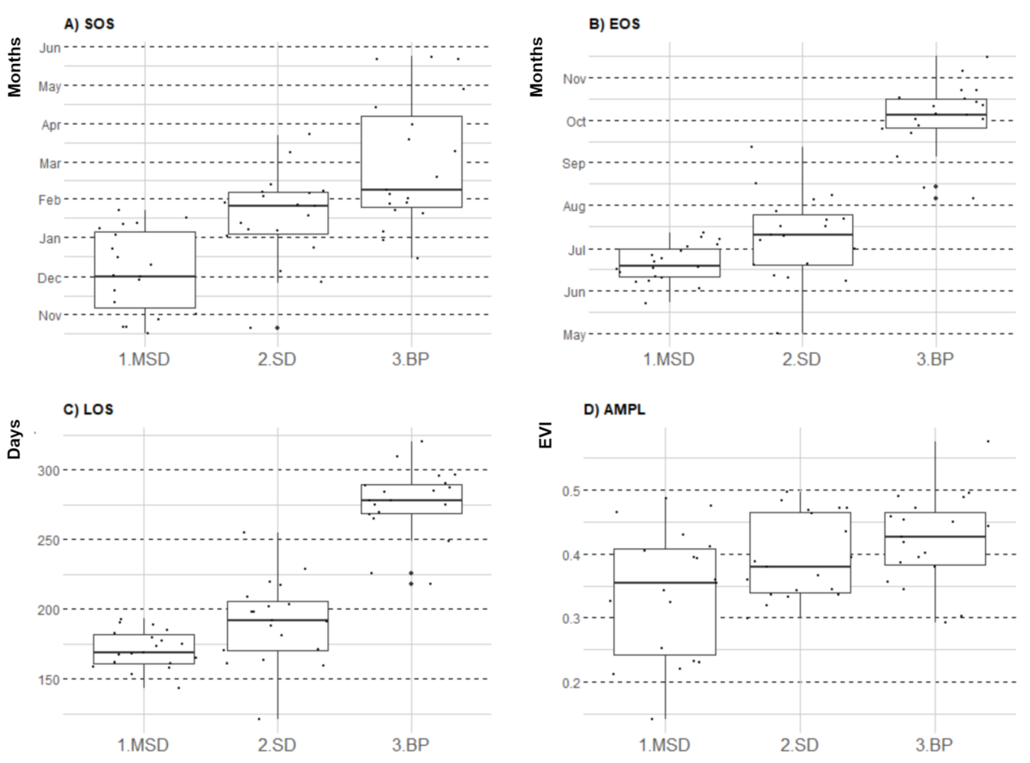
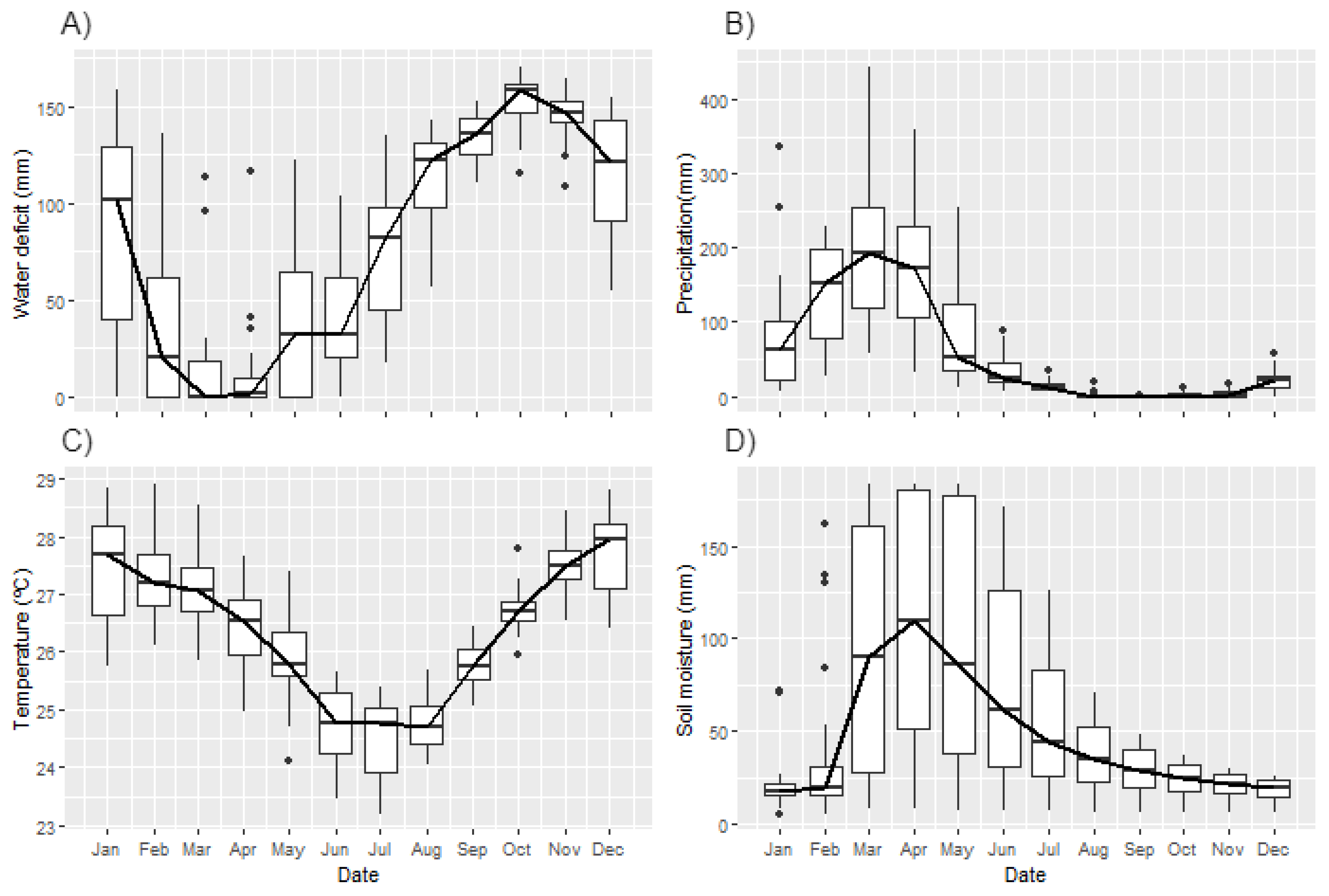
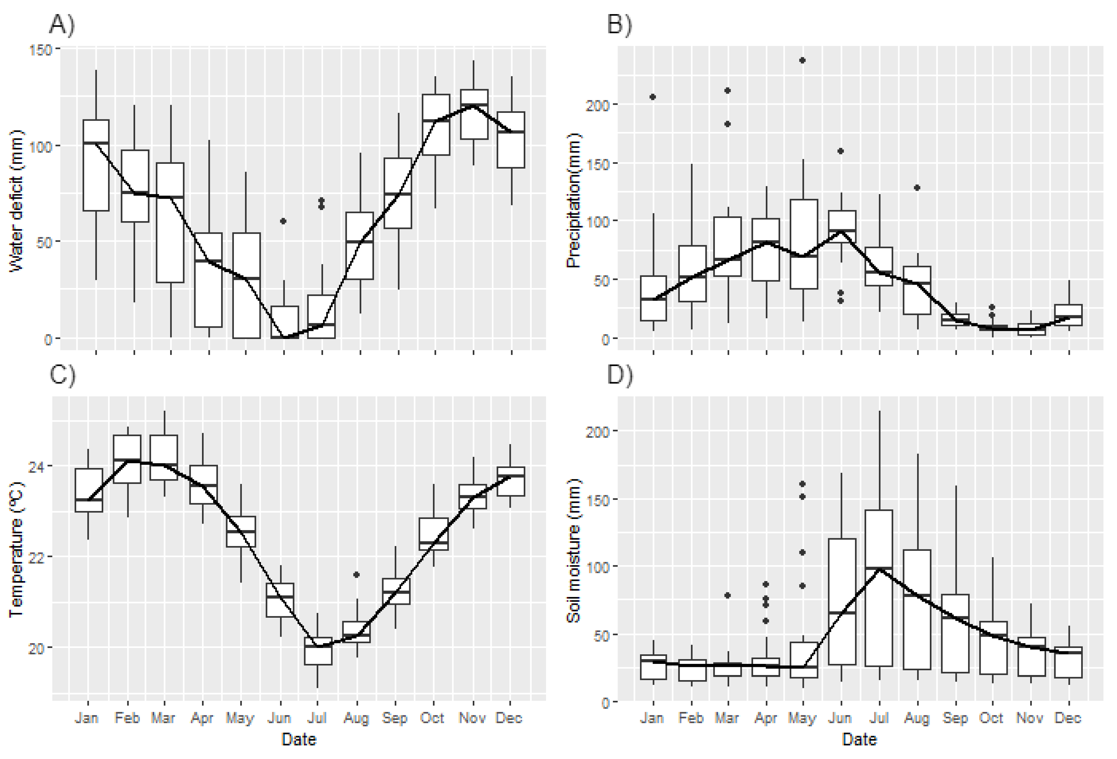
3.1. Seasonal Profiles and Phenology of SDTF Studied Sites

The interannual variability did not differ among sites for the SOS (X2 = 1.0; df = 2; p-value = 0.606) nor the EOS (X2 = 1.3; df = 2; p-value = 0.520). The variability was higher for the SOS than the EOS at MSD (X2 = 10.6; df = 1; p-value = 0.001) and BP (X2 = 11.1; df = 1; p-value = 0.0008) but not for SD (X2 = 0.8; df = 1; p-value = 0.363). The LOS differed among sites (F2,54 = 4.1; p-value = 0.02), with SD presenting a shorter LOS than BP (p-value = 0.01) but with no differences between MSD vs. BP (p-value = 0.37) and MSD vs. SD (p-value = 0.28). The amplitude of EVI also differed among sites (F2,54 = 5.2; p-value = 0.008), with MSD presenting lower amplitude than BP (p-value = 0.006) but with no differences between SD vs. BP (p-value = 0.52) and MSD vs. SD (p-value = 0.10).
The monthly values of the seasonal EVI profile for each ecoregion studied using 20 years of time series are presented in the box plot of Figure 2. The continuous line on the boxplot indicates the median of the monthly values for 20 years of the EVI time series. It can be seen in Figure 2 that the median values are always between 0.2 and 0.5. Despite the similarity in the amplitude of the EVI values, the graph of the median of the monthly values has different temporal behaviour for the different ecoregions studied. The maximum values on the MSD experimental site are similar in February and March. The monthly median presents a well-defined maximum value for the SD experimental site, occurring in April. The maximum EVI values occur in May and June at the BP experimental site. For MSD and SD studied ecoregions, the minimum values occur between six and seven months after the maximum values are observed, while for BP, it happens after four to five months.
Although the graphs with the monthly EVI values presented in Figure 2 understand the temporal behaviour, they do not reveal as many characteristics about the vegetation as the graphs with the phenological metrics presented in Figure 3. When analysing the SOS, it is noticed that the BP and MSD experimental sites present a greater interquartile range when compared to the SD experimental site. For most observations, the SOS from the SD experimental site has taken place between January and February. On the MSD experimental site, it is observed that SOS occurs most frequently between November and January. At BP, it is observed that the highest frequency of SOS occurs between January and May (117 days).
Interestingly, the interquartile range observed for the SOS is not for the EOS and LOS metrics for the MSD and BP experimental sites. For the EOS and LOS, it was observed that the MSD and BP sites have a smaller interquartile range than the SD experimental site, with interquartile range values of less than 30 days for both situations. For the SD experimental site, the variation in the interquartile range in the EOS is similar to that observed for SOS, with a variation slightly greater than 30 days interval and the LOS reaching an interquartile range of 60 days. A relationship of the amplitude with the other metrics, SOS, EOS, and LOS, was not observed. The amplitude’s highest values were observed for the BP and SD experimental sites, with 25% of the observations above 0.46. The amplitude values for the MSD experimental area had 75% of the observations below 0.31.

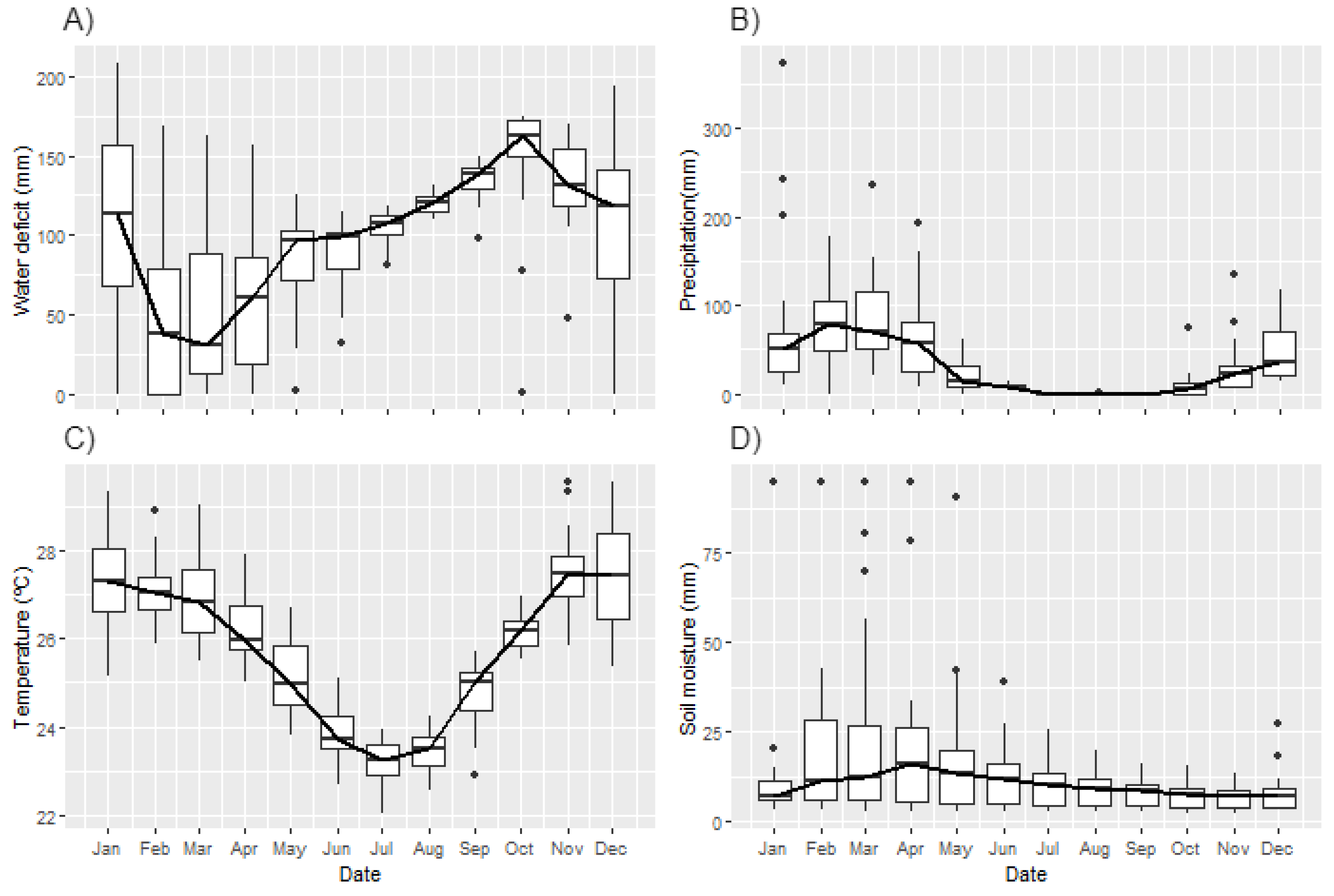
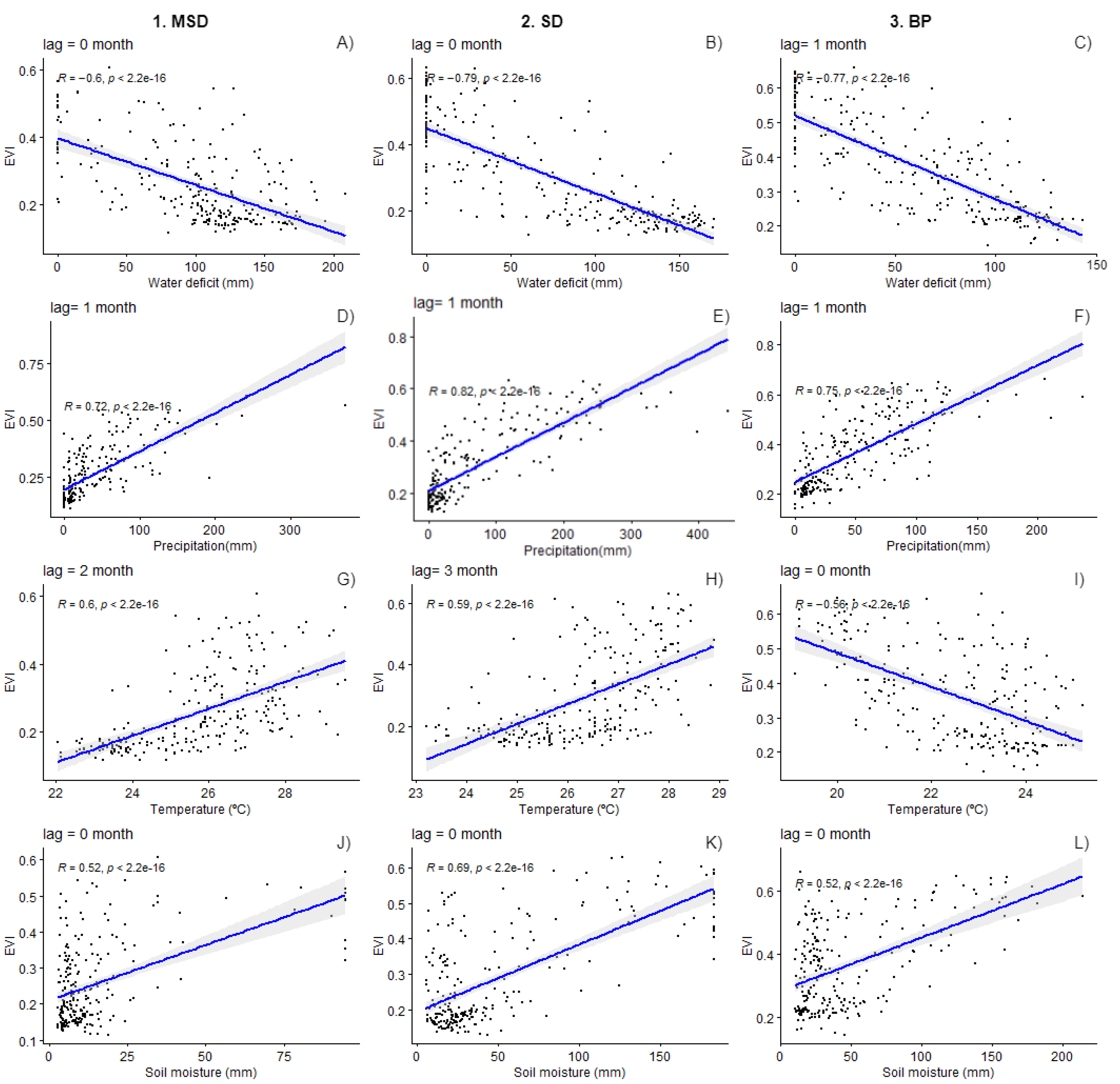
3.2. Environmental Drivers

Due to the high number of deciduous species, the SDTF, such as the Caatinga, presents high variability in plant biomass in the annual cycle. Figure 4, Figure 5 and Figure 6 present the environmental drivers’ boxplots that may influence the triggers of phenological changes in the Caatinga. When observing the shape of the graphs of the median behaviour of each environmental driver, it can be seen that there is a similarity in the water deficit, precipitation, and soil moisture behaviour. Pearson’s correlation coefficient for the environmental drivers and time series EVI is presented in Figure 7. Figure 7 only presents the lag (0–3 months) environmental drivers with the highest Pearson’s correlation. With the application of Pearson’s correlation, this study allowed for analysis of each environmental driver and identified their action times on vegetation. These results reinforce the importance of precipitation as the environmental driver that best reflects plant biomass production in the Caatinga. Thus, it is the environmental driver that presents the highest coefficient correlation among all: MSD (r = 0.7258; p < 0.05, lag = 1), SD (r = 0.8267; p < 0.05, lag = 1), and BP (r = 0.7546; p < 0.05, lag = 1). Subsequently, water deficit and soil moisture had the highest correlation values. The water deficit’s correlations were: MSD (r = −0.6, p < 0.01, lag = 0); SD (r = −0.79, p < 0.01, lag = 0); BP (r = −0.69, p < 0.01, lag = 1). Soil moisture is one of the main environmental triggers of the Caatinga, and in shallow soils, there is a tendency to saturate and also dry out more quickly, not allowing, in many cases, a long-term response from the vegetation: MSD (r = 0.52; p < 0.05, lag = 0), SD (r = 0.69; p < 0.05, lag = 0) and BP (r = 0.52; p < 0.05, lag = 0). Pearson’s correlation coefficient between the EVI and air temperature time series showed the weakest but most significant correlation. While MSD and SD presented positive relations between EVI and temperature (r = 0.6; p < 0.05, lag = 2) and (r = 0.59; p < 0.05, lag = 3), BP (r = −0.56; p < 0.05, lag = 0) showed a negative association.
In Pearson’s correlation, environmental drivers were analysed one by one. However, the observed behaviour may not reflect the actual effects on vegetation represented by the EVI time series. There may be an association of impact between the analysed environmental drivers. Partial correlation analysis is a way to solve this problem, allowing the analysis of multiple variables. The partial correlation analysis between the environmental drivers and EVI is presented in Table 1 with five scenarios. Scenario 1 considers all environmental drivers to calculate partial correlations, and in the other scenarios, the effect of one of the drivers is retained. Precipitation and soil moisture always showed a positive partial correlation. In contrast, the water deficit showed negative correlations, with r values ranging from −0.25 to −0.62. Only at the BP site, the partial correlation with temperature was negative. In scenario 1, with all environmental drivers, precipitation was the environmental driver that presented the highest correlation, with r values ranging from 0.48 to 0.51. The other environmental drivers are better perceived when precipitation is removed from the analysis (scenario 2). In scenario 2, the highest correlations were for temperature in MSD (0.46), water deficit and soil moisture for SD (0.40), and water deficit for BP (−0.62). This dependence relationship becomes evident when the drivers with the highest partial correlation identified in scenario 2 are removed from the analysis. Thus, the highest values of r for precipitation are seen in scenarios 5, 3, and 4 for MSD, SD, and BP sites, respectively.

4. Discussion

Compared to the following season, the greater rainfall variability at the beginning of the wet season may be the primary driver for the interquartile range of the SOS to be greater than that observed for the EOS and LOS (Figure 3). The higher frequency and accumulation are the main characteristics of rainfall contributing to the higher AMPL and LOS values at the BP experimental site. The partial coefficient of air temperature in the BP experimental site was always lower. In tropical regions, the air temperature variability is low, with about four degrees of annual amplitude difference from the monthly normal. However, in the MSD experimental site, there was a greater partial correlation between air temperature (scenario 2). The climatological water deficit is calculated from the reference evapotranspiration and precipitation, providing an efficient measure of the water availability and demand of the environment. Air temperature, directly related to water vapour-pressure deficit, is one of the climatic factors contributing to the variability of reference evapotranspiration [62]. The average monthly precipitation is quite variable in the annual cycle, which has a greater impact on the water deficit.
In the Caatinga, vegetation’s phenology and photosynthetic activity are associated with water availability [9]. In drier regions such as MSD and SD, intra-annual water availability is lower, leading to shorter growing season periods. The water stress makes the environmental conditions (Figure 2 and Figure 3) harsh for leaf maintenance for vegetation. In contrast, BP with more regular water availability (Figure 2 and Figure 3) shows larger LOS, which means more water and carbon exchange time at the soil–vegetation–atmosphere interface [63]. Carbon assimilation was related to EVI at Caatinga by Mendes et al. [64], demonstrating that the vegetation presents more significant photosynthetic activity and productivity (seasonal and total) during high EVI value periods. The vegetation at BP showed a higher senescence rate than in the other areas. The phenological parameter is related to leaf loss in the dry season and the maximum use of water availability for its recovery after the dry period with accelerated regrowth and increased metabolic processes in the rainy season [65]. These vegetation strategies are adaptive to optimise the phenological, vegetative, and reproductive processes [10]. The study areas showed similarities in the seasonality of phenological parameters, corroborating the high association level with water availability.
Many studies have shown that rainfall seasonality regulates SDTF canopy seasonality [24,66], but there is a complex relationship between environmental drivers and the vegetation response [9,28], mainly for the Caatinga where the plant physiology is adapted to drought and elevated temperatures [67]. As expected for the Caatinga vegetation, the months with the highest water deficit have the lowest leaf cover (lowest EVI values), a result previously found by other studies in the region [7,33,68]. About 70% of the year has a water deficit [69]. According to Flerchinger et al. [70], about 90% of the rainwater in arid and semi-arid regions returns to the atmosphere through evapotranspiration. As there is not such a significant variability in the average air temperature between the tropics, the annual constancy provides a high evaporative demand from the atmosphere throughout the year [69], conditioning the water deficit to the seasonal fluctuation of the rainfall, adjusting the Caatinga phenological cycle to the water availability. Phenological transitions are an excellent indicator of climate change [71], and future scenarios estimate greater water demand from plants and the occurrence of droughts, providing a more significant water deficit [72,73], and with that, being able to alter the phenology of the plants. The water deficit slows down plants’ growth, causes leaves, fruits, and flowers to fall, and, in the short term, tends to anticipate flowering and the beginning of fruiting, reducing plant cycles. In contrast, they tend to extend or even prevent the regular completion of the plant cycle [74].
The months with the highest spectral response of vegetation occurred in the rainy season when rain and soil moisture were predominantly distributed. The peak of the EVI was preceded by the month of greatest precipitation at SD and MSD. The rain at the BP experimental site shows a smoother and more regular distribution than in other areas, with the EVI closely following seasonal fluctuations in precipitation. The ecosystem accumulates sufficient water reserves in the soil and biomass for both sites under study, resulting in slower leaf fall during the dry season. The EVI followed the monthly rainfall distributions linearly, as shown in Figure 4. Likewise, the air temperature is observed after the maximum peak of the EVI. The air temperature also decreases the vegetation response, resulting in greater water stress for the research areas. Because of the high diversity of species at the Caatinga, the studied sites could present plants at different stages of adaptation or with physiological aspects related to water uptake or leaf abscission. The fact that MSD and SD present shorter LOS than BP could be related to vegetation strategies to use the water more efficiently during the available period. The peak of EVI values was higher at MSD and SD, and this would be related to more biomass production resulting from the water use efficiency (WUE) of the species composition.

5. Conclusions

This study observed that using the EVI time series efficiently estimated phenological parameters. The determination of the phenological parameters for 20 years allowed the evaluation of their seasonality. The seasonality of Caatinga vegetation growth differed between the three experimental sites. The SOS was the parameter that presented the greatest variability in the days of the year (DOY), reaching a variation of 117 days. The high variability of SOS occurred in sites with low variability of EOS and vice versa. The relationship between air temperature and vegetation was insignificant for the two experimental sites and presented a significant value for the site drier (MSD). At the experimental site where the highest vegetative peak co-occurred with the low air temperature, the highest LOS and AMPL were observed. In addition, the values of LOS and AMPL are directly linked to the annual distribution of rainfall, and the longer the rainy season, the greater their values are. The variability of the natural cycles of the environmental drivers that regulate the ecosystem’s phenology and the influence on the Caatinga’s natural dynamics indicated a greater sensitivity of the vegetation to water availability, with the water deficit being the limiting factor of the vegetation. There is a greater need for new research and studies aiming to reduce the impact of climatic risks by characterising and quantifying species’ response patterns to likely climate change. There will be changes in phenological patterns, production, and spatial distribution. Quantifying these impacts and devising appropriate actions to minimise such adversities represent significant research challenges in the coming decades.

Author Contributions

Formal analysis, R.M., J.A., M.M., A.M.P.-M. and C.A.C.d.S.; Investigation, R.M., J.A., M.M. and B.B.d.S.; Methodology, D.R. and J.C.; Software, R.M., J.A. and D.R.; Supervision, J.C.; Visualization, A.M.P.-M., C.A.C.d.S. and B.B.d.S.; Writing—original draft, R.M., J.A., D.R. and B.B.d.S.; Writing—review & editing, D.R., M.M., C.A.C.d.S. and J.C. All authors have read and agreed to the published version of the manuscript.

Funding

The study was financed by the Pró-Reitoria de Pós-Graduação e Pesquisa of the Federal University of Campina Grande (PRPG-UFCG), through of grant FAPESQ/Edital 04/2022, Paraíba State Research Foundation (FAPESQ).

Acknowledgments

The authors thank the Coordenação de Aperfeiçoamento de Pessoal de Nível Superior-Brazil (CAPES)-Finance Code 001 for the as a Brazilian CAPES scholarship to the first and second author, the project Nova geração de modelos para estimativas de evapotranspiração para o Semiárido Brasileiro (CNPq Proc. 409341/2021-5). This work forms part of the project Evolução na representação do balanço de energia por meio da integração de dados de campo e satélite aplicados a computação em nuvem para o semiárido brasileiro (FAPESQ under startup grant number #010/2021). The authors are also grateful to CNPq for the PQ (Productivity and Research) grants to the sixth autor (Proc. 304493/2019-8).

Conflicts of Interest

The authors declare no conflict of interest.

References

  1. Pennington, R.T.; Lehmann, C.; Rowland, L.M. Tropical savannas and dry forests. Curr. Biol. 2018, 28, R541–R545. [Google Scholar] [CrossRef] [PubMed] [Green Version]
  2. Moro, M.F.; Nic Lughadha, E.; de Araújo, F.S.; Martins, F.R. A Phytogeographical Metaanalysis of the Semiarid Caatinga Domain in Brazil. Bot. Rev. 2016, 82, 91–148. [Google Scholar] [CrossRef]
  3. De Queiroz, L.P.; Cardoso, D.; Fernandes, M.F.; Moro, M.F. Diversity and Evolution of Flowering Plants of the Caatinga Domain. Caatinga 2017, 23–63. [Google Scholar] [CrossRef]
  4. Fernandes, M.F.; Cardoso, D.; de Queiroz, L.P. An updated plant checklist of the Brazilian Caatinga seasonally dry forests and woodlands reveals high species richness and endemism. J. Arid Environ. 2020, 174, 104079. [Google Scholar] [CrossRef]
  5. Leith, H. Phenology and Seasonality Modeling. Soil Sci. 1974, 120, 461. [Google Scholar] [CrossRef]
  6. Morisette, J.T.; Richardson, A.D.; Knapp, A.K.; Fisher, J.I.; Graham, E.A.; Abatzoglou, J.; Wilson, B.E.; Breshears, D.D.; Henebry, G.M.; Hanes, J.M.; et al. Tracking the rhythm of the seasons in the face of global change: Phenological research in the 21st century. Front. Ecol. Environ. 2009, 7, 253–260. [Google Scholar] [CrossRef] [Green Version]
  7. Machado, I.C.S.; Barros, L.M.; Sampaio, E.V.S.B. Phenology of Caatinga Species at Serra Talhada, PE, Northeastern Brazil. Biotropica 1997, 29, 57–68. [Google Scholar] [CrossRef]
  8. Alberton, B.; Torres, R.D.S.; Cancian, L.F.; Borges, B.D.; Almeida, J.; Mariano, G.C.; dos Santos, J.; Morellato, P. Introducing digital cameras to monitor plant phenology in the tropics: Applications for conservation. Perspect. Ecol. Conserv. 2017, 15, 82–90. [Google Scholar] [CrossRef]
  9. Paloschi, R.; Ramos, D.; Ventura, D.; Souza, R.; Souza, E.; Morellato, L.; Nóbrega, R.; Coutinho, I.A.C.; Verhoef, A.; Körting, T.; et al. Environmental Drivers of Water Use for Caatinga Woody Plant Species: Combining Remote Sensing Phenology and Sap Flow Measurements. Remote Sens. 2020, 13, 75. [Google Scholar] [CrossRef]
  10. Vico, G.; Thompson, S.E.; Manzoni, S.; Molini, A.; Albertson, J.D.; Almeida-Cortez, J.S.; Fay, P.A.; Feng, X.; Guswa, A.J.; Liu, H.; et al. Climatic, ecophysiological, and phenological controls on plant ecohydrological strategies in seasonally dry ecosystems. Ecohydrology 2015, 8, 660–681. [Google Scholar] [CrossRef] [Green Version]
  11. Riahi, K.; Schaeffer, R.; Arango, J.; Calvin, K.; Guivarch, C.; Hasegawa, T.; Jiang, K.; Kriegler, E.; Matthews, R.; Peters, G.P.; et al. Mitigation pathways compatible with long-term goals. In IPCC, 2022: Climate Change 2022: Mitigation of Climate Change. Contribution of Working Group III to the Sixth Assessment Report of the Intergovernmental Panel on Climate Change; Shukla, P.R., Skea, J., Slade, R., Al Khourdajie, A., van Diemen, R., McCollum, D., Pathak, M., Some, S., Vyas, P., Fradera, R., et al., Eds.; Cambridge University Press: Cambridge, UK; New York, NY, USA, 2022. [Google Scholar] [CrossRef]
  12. Torres, R.R.; Lapola, D.M.; Gamarra, N.L.R. Future Climate Change in the Caatinga. Caatinga 2017, 383–410. [Google Scholar] [CrossRef]
  13. Marengo, J.A.; Cunha, A.P.M.A.; Nobre, C.A.; Neto, G.G.R.; Magalhaes, A.R.; Torres, R.R.; Sampaio, G.; Alexandre, F.; Alves, L.M.; Cuartas, L.A.; et al. Assessing drought in the drylands of northeast Brazil under regional warming exceeding 4 °C. Nat. Hazards 2020, 103, 2589–2611. [Google Scholar] [CrossRef]
  14. Xu, L.; Myneni, R.; Iii, F.S.C.; Callaghan, T.V.; Pinzon, J.E.; Tucker, C.J.; Zhu, Z.; Bi, J.; Ciais, P.; Tømmervik, H.; et al. Temperature and vegetation seasonality diminishment over northern lands. Nat. Clim. Chang. 2013, 3, 581–586. [Google Scholar] [CrossRef] [Green Version]
  15. Tong, X.; Tian, F.; Brandt, M.; Liu, Y.; Zhang, W.; Fensholt, R. Trends of land surface phenology derived from passive microwave and optical remote sensing systems and associated drivers across the dry tropics 1992–2012. Remote Sens. Environ. 2019, 232. [Google Scholar] [CrossRef]
  16. Brando, P.M.; Goetz, S.J.; Baccini, A.; Nepstad, D.C.; Beck, P.S.A.; Christman, M.C. Seasonal and interannual variability of climate and vegetation indices across the Amazon. Proc. Natl. Acad. Sci. USA 2010, 107, 14685–14690. [Google Scholar] [CrossRef] [Green Version]
  17. Olmos-Trujillo, E.; González-Trinidad, J.; Júnez-Ferreira, H.; Pacheco-Guerrero, A.; Bautista-Capetillo, C.; Avila-Sandoval, C.; Galván-Tejada, E. Spatio-Temporal Response of Vegetation Indices to Rainfall and Temperature in A Semiarid Region. Sustainability 2020, 12, 1939. [Google Scholar] [CrossRef] [Green Version]
  18. Andrade, J.; Cunha, J.; Silva, J.; Rufino, I.; Galvão, C. Evaluating single and multi-date Landsat classifications of land-cover in a seasonally dry tropical forest. Remote Sens. Appl. Soc. Environ. 2021, 22, 100515. [Google Scholar] [CrossRef]
  19. Huete, A.; Didan, K.; Miura, T.; Rodriguez, E.P.; Gao, X.; Ferreira, L.G. Overview of the radiometric and biophysical performance of the MODIS vegetation indices. Remote Sens. Environ. 2002, 83, 195–213. [Google Scholar] [CrossRef]
  20. Adole, T.; Dash, J.; Atkinson, P. A systematic review of vegetation phenology in Africa. Ecol. Inform. 2016, 34, 117–128. [Google Scholar] [CrossRef]
  21. Suepa, T.; Qi, J.; Lawawirojwong, S.; Messina, J. Understanding spatio-temporal variation of vegetation phenology and rainfall seasonality in the monsoon Southeast Asia. Environ. Res. 2016, 147, 621–629. [Google Scholar] [CrossRef] [Green Version]
  22. Htitiou, A.; Boudhar, A.; Lebrini, Y.; Hadria, R.; Lionboui, H.; Elmansouri, L.; Tychon, B.; Benabdelouahab, T. The Performance of Random Forest Classification Based on Phenological Metrics Derived from Sentinel-2 and Landsat 8 to Map Crop Cover in an Irrigated Semi-arid Region. Remote Sens. Earth Syst. Sci. 2019, 2, 208–224. [Google Scholar] [CrossRef]
  23. Pastor-Guzman, J.; Dash, J.; Atkinson, P. Remote sensing of mangrove forest phenology and its environmental drivers. Remote Sens. Environ. 2018, 205, 71–84. [Google Scholar] [CrossRef] [Green Version]
  24. De Jesus, J.B.; Kuplich, T.M.; Barreto, D.D.C.; da Rosa, C.N.; Hillebrand, F.L. Temporal and phenological profiles of open and dense Caatinga using remote sensing: Response to precipitation and its irregularities. J. For. Res. 2021, 32, 1067–1076. [Google Scholar] [CrossRef]
  25. Songsom, V.; Koedsin, W.; Ritchie, R.J.; Huete, A. Mangrove Phenology and Environmental Drivers Derived from Remote Sensing in Southern Thailand. Remote Sens. 2019, 11, 955. [Google Scholar] [CrossRef] [Green Version]
  26. Wang, G.; Huang, Y.; Wei, Y.; Zhang, W.; Li, T.; Zhang, Q. Inner Mongolian grassland plant phenological changes and their climatic drivers. Sci. Total Environ. 2019, 683, 1–8. [Google Scholar] [CrossRef]
  27. Huang, J.-G.; Ma, Q.; Rossi, S.; Biondi, F.; Deslauriers, A.; Fonti, P.; Liang, E.; Mäkinen, H.; Oberhuber, W.; Rathgeber, C.B.K.; et al. Photoperiod and temperature as dominant environmental drivers triggering secondary growth resumption in Northern Hemisphere conifers. Proc. Natl. Acad. Sci. USA 2020, 117, 20645–20652. [Google Scholar] [CrossRef]
  28. Godoy-Veiga, M.; Cintra, B.B.L.; Stríkis, N.M.; Cruz, F.W.; Grohmann, C.H.; Santos, M.S.; Regev, L.; Boaretto, E.; Ceccantini, G.; Locosselli, G.M. The value of climate responses of individual trees to detect areas of climate-change refugia, a tree-ring study in the Brazilian seasonally dry tropical forests. For. Ecol. Manag. 2021, 488, 118971. [Google Scholar] [CrossRef]
  29. Whitecross, M.; Witkowski, E.; Archibald, S. No two are the same: Assessing variability in broad-leaved savanna tree phenology, with watering, from 2012 to 2014 at Nylsvley, South Africa. S. Afr. J. Bot. 2016, 105, 123–132. [Google Scholar] [CrossRef]
  30. Ryan, C.M.; Williams, M.; Grace, J.; Woollen, E.; Lehmann, C.E.R. Pre-rain green-up is ubiquitous across southern tropical Africa: Implications for temporal niche separation and model representation. New Phytol. 2016, 213, 625–633. [Google Scholar] [CrossRef] [Green Version]
  31. Sampaio, E.V. Overview of the Brazilian caatinga. Seas. Dry Trop. For. 1995, 1, 35–63. [Google Scholar] [CrossRef]
  32. Gutiérrez, A.P.A.; Engle, N.L.; De Nys, E.; Molejón, C.; Martins, E.S. Drought preparedness in Brazil. Weather Clim. Extremes 2014, 3, 95–106. [Google Scholar] [CrossRef] [Green Version]
  33. Alberton, B.; Torres, R.D.S.; Silva, T.S.F.; da Rocha, H.R.; Moura, M.S.B.; Morellato, L.P.C. Leafing Patterns and Drivers across Seasonally Dry Tropical Communities. Remote Sens. 2019, 11, 2267. [Google Scholar] [CrossRef] [Green Version]
  34. Alvares, C.A.; Stape, J.L.; Sentelhas, P.C.; Moraes, G.J.L.; Sparovek, G. Köppen’s climate classification map for Brazil. Meteorol. Z. 2013, 22, 711–728. [Google Scholar] [CrossRef]
  35. Sampaio, E.V.S.B. Características e potencialidades. In Uso Sustentável e Conservação dos Recursos Florestais da Caatinga; Gariglio, M.A., Sampaio, E.V.S.B., Cestaro, L.A., Kageyama, P.Y., Eds.; Serviço Florestal Brasileiro: Brasília, Brazil, 2010; pp. 29–48. [Google Scholar]
  36. Prado, D. As caatingas da América do Sul. In Ecologia e Conservação da Caatinga; Leal, I.R., Tabarelli, M., Silva, J.M.C., Eds.; Universitária da UFPE: Recife, Brazil, 2003; pp. 3–73. [Google Scholar]
  37. Nimer, E. Climatologia da região Nordeste do Brasil. Introdução à climatologia dinâmica. Rev. Bras. Geogr. 1972, 34, 3–51. [Google Scholar]
  38. Velloso, A.L.; Sampaio, E.V.S.B.; Giulietti, A.M.; Barbosa, M.R.V.; Castri, A.A.J.F.; Queiroz, L.P.; Fernandes, A.; Oren, D.C.; Cestaro, L.A.; Carvalho, A.J.E.; et al. Ecorregiões: Propostas para o Bioma Caatinga. In Associação Plantas do Nordeste; The Nature Conservancy do Brasil: Recife, Brazil, 2002; p. 75. [Google Scholar]
  39. Souza, R.; Feng, X.; Antonino, A.; Montenegro, S.; Souza, E.; Porporato, A. Vegetation response to rainfall seasonality and interannual variability in tropical dry forests. Hydrol. Process. 2016, 30, 3583–3595. [Google Scholar] [CrossRef]
  40. Kill, L.H.P. Caracterização da vegetação da Reserva Legal da Embrapa Semiárido. Embrapa Semiárido Pet. 2017, 1, 1–27. [Google Scholar]
  41. Tavares-Damasceno, J.P.; Silveira, J.L.G.D.S.; Câmara, T.; Stedile, P.D.C.; Macario, P.; Toledo-Lima, G.S.; Pichorim, M. Effect of drought on demography of Pileated Finch (Coryphospingus pileatus: Thraupidae) in northeastern Brazil. J. Arid Environ. 2017, 147, 63–70. [Google Scholar] [CrossRef]
  42. Althoff, T.D.; Menezes, R.; de Carvalho, A.L.; Pinto, A.D.S.; Santiago, G.A.C.F.; Ometto, J.; Von Randow, C.; Sampaio, E.V.D.S.B. Climate change impacts on the sustainability of the firewood harvest and vegetation and soil carbon stocks in a tropical dry forest in Santa Teresinha Municipality, Northeast Brazil. For. Ecol. Manag. 2016, 360, 367–375. [Google Scholar] [CrossRef]
  43. Cunha, J.E.B.L.; Rufino, I.A.A.; Ideião, S.M.A. Determinação da temperatura da superfície na cidade de Campina Grande-PB a partir de imagens do satélite Landsat 5-TM. In Anais XIV Simpósio Brasileiro de Sensoriamento Remoto; INPE: Natal, Brazil, 2009. [Google Scholar]
  44. INMET, National Institute of Meteorology of Brazil, 2021. Available online: https://bdmep.inmet.gov.br/# (accessed on 1 October 2021).
  45. Embrapa, Empresa Brasileira de Pesquisa Aagropecuária. Centro Nacional de Pesquisa de Solos. Sistema Brasileiro de Classificação de Solo, 2nd ed.; Embrapa Solos: Rio de Janeiro, Brazil, 2006. [Google Scholar]
  46. Gorelick, N.; Hancher, M.; Dixon, M.; Ilyushchenko, S.; Thau, D.; Moore, R. Google Earth Engine: Planetary-scale geospatial analysis for everyone. Remote Sens. Environ. 2017, 202, 18–27. [Google Scholar] [CrossRef]
  47. Guerschman, J.P.; Scarth, P.F.; McVicar, T.R.; Renzullo, L.J.; Malthus, T.J.; Stewart, J.B.; Rickards, J.E.; Trevithick, R. Assessing the effects of site heterogeneity and soil properties when unmixing photosynthetic vegetation, non-photosynthetic vegetation and bare soil fractions from Landsat and MODIS data. Remote Sens. Environ. 2015, 161, 12–26. [Google Scholar] [CrossRef]
  48. Abatzoglou, J.T.; Dobrowski, S.; Parks, S.A.; Hegewisch, K.C. TerraClimate, a high-resolution global dataset of monthly climate and climatic water balance from 1958–2015. Sci. Data 2018, 5, 170191. [Google Scholar] [CrossRef] [PubMed] [Green Version]
  49. Funk, C.; Peterson, P.; Landsfeld, M.; Pedreros, D.; Verdin, J.; Shukla, S.; Husak, G.; Rowland, J.; Harrison, L.; Hoell, A.; et al. The climate hazards infrared precipitation with stations—A new environmental record for monitoring extremes. Sci. Data 2015, 2, 150066. [Google Scholar] [CrossRef] [PubMed] [Green Version]
  50. Jönsson, P.; Eklundh, L. TIMESAT—A program for analyzing time-series of satellite sensor data. Comput. Geosci. 2004, 30, 833–845. [Google Scholar] [CrossRef] [Green Version]
  51. Jönsson, P.; Eklundh, L. TIMESAT 3.1—Software Manual; Lund University: Lund, Sweden, 2012; p. 82. Available online: http://web.nateko.lu.se/timesat/timesat.asp (accessed on 1 May 2021).
  52. Savitzky, A.; Golay, M.J.E. Smoothing and Differentiation of Data by Simplified Least Squares Procedures. Anal. Chem. 1964, 36, 1627–1639. [Google Scholar] [CrossRef]
  53. Kong, F.; Li, X.; Wang, H.; Xie, D.; Li, X.; Bai, Y. Land Cover Classification Based on Fused Data from GF-1 and MODIS NDVI Time Series. Remote Sens. 2016, 8, 741. [Google Scholar] [CrossRef] [Green Version]
  54. Streher, A.S.; Sobreiro, J.F.F.; Morellato, P.; Silva, T. Land Surface Phenology in the Tropics: The Role of Climate and Topography in a Snow-Free Mountain. Ecosystems 2017, 20, 1436–1453. [Google Scholar] [CrossRef] [Green Version]
  55. Diem, P.K.; Pimple, U.; Sitthi, A.; Varnakovida, P.; Tanaka, K.; Pungkul, S.; Leadprathom, K.; LeClerc, M.Y.; Chidthaisong, A. Shifts in Growing Season of Tropical Deciduous Forests as Driven by El Niño and La Niña during 2001–2016. Forests 2018, 9, 448. [Google Scholar] [CrossRef] [Green Version]
  56. Wang, Y.; Zang, S.; Tian, Y. Mapping paddy rice with the random forest algorithm using MODIS and SMAP time series. Chaos Solitons Fractals 2020, 140. [Google Scholar] [CrossRef]
  57. Ramírez-Cuesta, J.; Minacapilli, M.; Motisi, A.; Consoli, S.; Intrigliolo, D.; Vanella, D. Characterization of the main land processes occurring in Europe (2000–2018) through a MODIS NDVI seasonal parameter-based procedure. Sci. Total Environ. 2021, 799, 149346. [Google Scholar] [CrossRef]
  58. Doussoulin-Guzmán, M.-A.; Pérez-Porras, F.-J.; Triviño-Tarradas, P.; Ríos-Mesa, A.-F.; Porras, A.G.-F.; Mesas-Carrascosa, F.-J. Grassland Phenology Response to Climate Conditions in Biobio, Chile from 2001 to 2020. Remote Sens. 2022, 14, 475. [Google Scholar] [CrossRef]
  59. Conover, W.J.; Johnson, M.E.; Johnson, M.M. A Comparative Study of Tests for Homogeneity of Variances, with Applications to the Outer Continental Shelf Bidding Data. Technometrics 1981, 23, 351–361. [Google Scholar] [CrossRef]
  60. Zhu, W.; Zheng, Z.; Jiang, N.; Zhang, D. A comparative analysis of the spatio-temporal variation in the phenologies of two herbaceous species and associated climatic driving factors on the Tibetan Plateau. Agric. For. Meteorol. 2018, 248, 177–184. [Google Scholar] [CrossRef]
  61. R Development Core Team. R: A Language and Environment for Statistical Computing; R Foundation for Statistical Computing: Vienna, Austria, 2019; Available online: https://www.r-project.org (accessed on 20 February 2019).
  62. De Souza, L.S.B.; Silva, M.T.L.; Alba, E.; de Moura, M.S.B.; Neto, J.F.D.C.; de Souza, C.A.A.; da Silva, T.G.F. New method for estimating reference evapotranspiration and comparison with alternative methods in a fruit-producing hub in the semi-arid region of Brazil. Arch. Meteorol. Geophys. Bioclimatol. Ser. B 2022, 1–10. [Google Scholar] [CrossRef]
  63. Dos Santos, C.A.C.; Mariano, D.A.; Nascimento, F.D.C.A.D.; Dantas, F.R.D.C.; de Oliveira, G.; Silva, M.T.; da Silva, L.L.; da Silva, B.B.; Bezerra, B.G.; Safa, B.; et al. Spatio-temporal patterns of energy exchange and evapotranspiration during an intense drought for drylands in Brazil. Int. J. Appl. earth Obs. Geoinf. ITC J. 2019, 85, 101982. [Google Scholar] [CrossRef]
  64. Mendes, K.R.; Campos, S.; Da Silva, L.L.; Mutti, P.R.; Ferreira, R.R.; Medeiros, S.S.; Perez-Marin, A.M.; Marques, T.V.; Ramos, T.M.; Vieira, M.M.D.L.; et al. Seasonal variation in net ecosystem CO2 exchange of a Brazilian seasonally dry tropical forest. Sci. Rep. 2020, 10, 1–16. [Google Scholar] [CrossRef] [PubMed]
  65. Bezerra, M.V.C.; Da Silva, B.B.; Bezerra, B.G. Avaliação dos efeitos atmosféricos no albedo e NDVI obtidos com imagens de satélite. Rev. Bras. Eng. Agrícola Ambient. 2011, 15, 709–717. [Google Scholar] [CrossRef] [Green Version]
  66. Allen, K.; Dupuy, J.M.; Gei, M.G.; Hulshof, C.; Medvigy, D.; Pizano, C.; Salgado-Negret, B.; Smith, C.M.; Trierweiler, A.; Van Bloem, S.J.; et al. Will seasonally dry tropical forests be sensitive or resistant to future changes in rainfall regimes? Environ. Res. Lett. 2017, 12, 023001. [Google Scholar] [CrossRef] [Green Version]
  67. Trovão, D.M.D.B.M.; Fernandes, P.D.; De Andrade, L.A.; Neto, J.D. Variações sazonais de aspectos fisiológicos de espécies da Caatinga. Rev. Bras. Eng. Agrícola Ambient. 2007, 11, 307–311. [Google Scholar] [CrossRef] [Green Version]
  68. Miranda, R.D.Q.; Nóbrega, R.L.B.; de Moura, M.S.B.; Raghavan, S.; Galvíncio, J.D. Realistic and simplified models of plant and leaf area indices for a seasonally dry tropical forest. Int. J. Appl. Earth Obs. Geoinf. ITC J. 2020, 85, 101992. [Google Scholar] [CrossRef]
  69. Marengo, J.A.; Torres, R.R.; Alves, L.M. Drought in Northeast Brazil—past, present, and future. Theor. Appl. Climatol. 2016, 129, 1189–1200. [Google Scholar] [CrossRef]
  70. Flerchinger, G.N.; Hanson, C.L.; Wight, J.R. Modeling Evapotranspiration and Surface Energy Budgets across a Watershed. Water Resour. Res. 1996, 32, 2539–2548. [Google Scholar] [CrossRef]
  71. Langvall, O.; Löfvenius, M.O. Long-term standardized forest phenology in Sweden: A climate change indicator. Int. J. Biometeorol. 2021, 65, 381–391. [Google Scholar] [CrossRef] [PubMed] [Green Version]
  72. Marin, F.R.; Assad, E.D.; Barbarisi, B.F.; Pilau, F.G.; Pacheco, L.R.F.; Zullo, J.J.; Pinto, H.S. Efeito das mudanças climáticas sobre a aptidão climática para cana-de-açúcar no Estado de São Paulo. In Congresso Brasileiro de Agrometeorologia; Embrapa/SBAgro: Aracaju, Brazil, 2007; Volume 15. [Google Scholar]
  73. Nepomuceno, A.L.; Farias, J.R.B.; Salinet, L.H.; Polizel, A.M.; Neumaier, N.; Beneventi, M.A.; Stolf, R.; Rolla, A.A.P. Engenharia genética como ferramenta no desenvolvimento de plantas de soja adaptadas a cenários futuros de mudanças climáticas. In Congresso Brasileiro de Agrometeorologia; Embrapa/SBAgro: Aracaju, Brazil, 2007. [Google Scholar]
  74. Bergamaschi, H. O clima como fator determinante da fenologia das plantas. In Fenologia: Ferramenta para Conservação, Melhoramento e Manejo de Recursos Vegetais Arbóreos; Embrapa Florestas: Colombo, Brazil, 2007; Volume 1, pp. 291–310. [Google Scholar]
Figure 1. Map of the Caatinga with the physical boundaries of the ecoregions and the locations under study. Koppen’s climate classification for Brazil from ALVARES et al. [34] emphasizes the semi-arid (BSh) climate of Caatinga SDTF in orange. Location of sites in ecoregions: 1. MSD (Meridional Sertaneja Depression ecoregion); 2. SD (Sertanejas Depressions ecoregion); 3. BP (Borborema Plateau ecoregion).
Remotesensing 14 02637 g001
Figure 2. Monthly EVI values for 20 years of time series in (A) MSD ecoregion experimental, (B) SD ecoregion experimental, and (C) BP ecoregion experimental.
Remotesensing 14 02637 g002
Figure 3. Caatinga phenological metrics of the three ecoregions studied, (A) SOS, (B) EOS, (C) LOS, and (D) Amplitude.
Remotesensing 14 02637 g003
Figure 4. Environment drivers for MSD in (A) Water Deficit, (B) Precipitation, (C) Air Temperature, and (D) Soil moisture.
Remotesensing 14 02637 g004
Figure 5. Environment drivers for SD in (A) Water Deficit, (B) Precipitation, (C) Air Temperature, and (D) Soil moisture.
Remotesensing 14 02637 g005
Figure 6. Environment drivers for BP in (A) Water Deficit, (B) Precipitation, (C) Air Temperature, and (D) Soil moisture.
Remotesensing 14 02637 g006
Figure 7. Correlation between EVI and environment drivers for MSD, SD, and BP in water deficit (AC), precipitation (DF), air temperature (GI), and (D) Soil moisture (JL). The lag months have the highest (r2) between the environmental drivers and the EVI monthly time series.
Remotesensing 14 02637 g007
Table 1. Partial correlation coefficients between the EVI and environment drivers across MSD, SD, and BP sites. Scenario 1 considers all environmental drivers to calculate partial correlations. For the other scenarios, the effect of one of the variables is removed: scenarios 2 (without precipitation), 3 (without soil moisture), 4 (without water deficit), and 5 (without temperature). “-” indicates that the environment driver was not used to calculate the partial correlation. Only for statistical significance (p < 0.05). Missing estimates (NS) are not significant.
SiteScenariosAir Temperature (°C)Water Deficit (mm)Soil Moisture (mm)Precipitation (mm)
1. MSD10.28−0.25NS0.48
20.46−0.270.26-
30.26−0.34-0.52
40.34-0.260.49
5-−0.32NS0.58
2. SD10.09−0.410.110.51
20.26−0.400.40-
30.06−0.50-0.61
40.36-0.330.51
5-−0.520.080.55
3. BP1NS−0.290.180.48
2NS−0.620.16-
3−0.14−0.32-0.47
4−0.28-0.230.69
5-−0.390.220.48
Publisher’s Note: MDPI stays neutral with regard to jurisdictional claims in published maps and institutional affiliations.

