Mapping Climate Zones of Iran Using Hybrid Interpolation Methods

Abstract

Climate plays a key role in ecosystem services. Understanding microclimate change can be a significant help in making the right decision for ecosystems and buffering the effects of global warming. Given the large distances between meteorological stations and the changes in the climate variables within short distances, such variations cannot be detected just by using observed meteorological data. This study aimed at determining the spatial structure of the mean annual temperature, the annual average precipitation, and the climate zoning of Iran using data from 3825 stations from 2002 to 2016.The multivariate regression demonstrated the dependence of these variables on longitude, latitude, and elevation. Regression-kriging indicated a decline in temperature from east to west and northwest in high-altitude areas, while most precipitation values were observed over the Caspian Sea coastline and the Zagros Mountains. Climatic zoning showed that using auxiliary variables was very effective in detecting 24 climatic classes and understating the climate diversity in Iran. Hot to very hot and arid to very arid climate classes occupy the largest part of Iran, including the southeastern and southern desert regions. According to the generated climatic map, the large climatic diversity of Iran needs accurate policymaking regarding cultivation patterns and biodiversity. Visual comparisons of climatic zones with four remotely sensed agricultural-related variables showed that using such carefully produced climatic maps would be beneficial in classifying, assessing, and interpreting the remote sensed agricultural-related variables.

1. Introduction

Nearly one-third of Iran’s territory is covered by mountains. The main characteristics of the precipitation regimes in Iran include low annual precipitation, severe annual and seasonal fluctuations in precipitation, short precipitation periods, and heavy rainstorms. Precipitation does not follow a specific pattern in Iran and varies with location. Differences depend on the direction and origin of the air masses affecting Iran, as well as the mountain aspect [1]. The air temperature in Iran is considerably dependent on elevation, longitude, and latitude, the effect of elevation being considerably greater than that of the latitude. The climate in mountainous regions with a heterogeneous topography significantly changes due to the large elevation gradient over a short distance [2]. Large-scale temperature variations in the mountains are mainly dependent on physical processes such as airflow; solar radiation; and interactions with topographic complexities including aspect, roughness, and shape of the terrain [3]. Vegetation and geographical dispersion of humans locally affect the temperature [4]. Different climates have been formed in Iran due to the wide latitude and vegetation variations and different terrains, such as deserts, dense forests, coastal regions, and high mountains.

Depending on the development level, between 20 and 80% of the changes in annual agricultural products are due to weather fluctuations, so between 1 and 5% of agricultural products are lost because of changes in the weather, in addition to severe losses from indirect negative effects, such as pests and diseases [5].

Macroclimate data may be sufficient for plain physiographic units with small changes in land use, but the borders of climatic regions should be accurately delineated to explain the behaviors of animals and plants [6].

Fine-resolution climate data is required for the correct prediction of plant species and their behavior in natural and anthropogenic environments. It has been found that spatial nonuniformity in climate variables makes temperature calculated from the direct local measurements to be twice as much as that calculated through global interpolation techniques [7]. Spatial distribution models (SDMs) are increasingly growing around the world to respond to ecological questions ranging from climate changes to management challenges [4]. However, SDM predictions mainly rely on the conditions of coarse resolution synoptic stations and fail to consider fine-resolution climate classes, because most climate variations in large-scale mountainous regions act as fine-resolution models. Accordingly, it is necessary to combine data collected from synoptic stations with auxiliary variables to achieve a finer spatial variability of climate variables. In a study of spatial variability of daily weather variables in the High Plains of the USA that was undertaken in a multivariable network, it is shown that, to explain more than 90% of the variation in the maximum temperatures between sites, a spacing of 60 km was sufficient on a year-round basis, while the minimum temperature required closer spacing (~30 km) to achieve this criterion. The spacing of precipitation gauges, for this criterion, would be less than 5 km [8]. In another study, to eliminate the effect of uneven stations, using 736 meteorological station data (from 1961 to 2010) and the Inverse Weighted Distance (IDW) method, researchers detected the trends in climatic variables, including average precipitation, air temperature, solar radiation, and wind speed, for the whole of China and showed that there are three large-scale instrument replacements that increase the uncertainties of the trend analysis [9].

Given the large distance between small-scale synoptic and climatological stations and the climate, class variations are smaller than these distances, and despite the need for accurate temperature and precipitation data, these stations cannot present microclimatic classes adequately. Moreover, establishing denser meteorological stations, even mobile stations or individual sensors, will be costly. To access more correct data, a change in scale towards a finer scale, known as interpolation, may be necessary [10]. Multiple climate parameters used in traditional methods fail to represent the real climate classes. Many efforts have recently been made to provide a more realistic picture of the regional climate using geographical parameters. Additionally, the selection of auxiliary variables to increase the accuracy of climate zoning should result in a finer spatial resolution to take into account the mean, borders, and nonuniformity of the climatic variables [4].

Geostatistical interpolation methods are often used for the interpolation of climatic variables [11]. The kriging method models the spatial correlation of regional climatic variables (such as temperature and precipitation) using a semi-variogram. Changes in patterns of the spatial autocorrelation of the maximum temperatures of Iran were investigated in a study using 125 synoptic stations’ data (from 2010 to 1980) and kriging interpolation and showed areas with positive and negative spatial autocorrelations [12]. Regression-kriging(RK) combines climatic variable observations with auxiliary variables such as height for the optimal estimations [13]. The superiority of the regression-kriging method over conventional geostatistical methods in the interpolation of climatic variables has been shown in several studies [14,15,16]. In the Jalisco state of Mexico, seven geostatistical interpolation methods were evaluated in predicting the monthly maximum temperature and monthly mean precipitation, and the results showed that the regression-kriging and thin-plate spline were the most efficient methods [17]. In Extremadura, a region of Southwestern Spain, different geostatistical approaches to map climate variables were evaluated. In this study, the ordinary kriging (OK), simple kriging (SK), and universal kriging (universal kriging) methods were compared with three multivariate algorithms that take into account the altitude: collocated ordinary cokriging (OCK), simple kriging with varying local means (SKV), and regression-kriging (RK). The different techniques were applied to monthly and annual precipitation data measured at 136 meteorological stations in the region. Cross-validation showed that prediction performances vary among algorithms. SKV and RK provide the smallest MSE of estimates and, therefore, performed better. The SKV and RK maps are influenced by the DEM pattern and showed more details than the co-kriged maps [18]. To determine the best interpolation method for the annual and seasonal precipitation of the Mashhad Plain in Iran, rainfall data from 63 stations (from 2004 to 2013) were collected. Five interpolation methods, namely Kriging, co-Kriging, Regression, regression-kriging, and Inverse Weighted Distance (IDW), were used. The root mean square error (RMSE) and mean bias error (MBE) were considered to select the best interpolation method. The results revealed that the regression-kriging and three-variable regression (x, y, z) methods were the most accurate models to interpolate the annual precipitation over the study area [19]. In another study, regression-kriging was used to map the winter chilling hours of mainland Spain. Temperature data from 72 meteorological stations (from 1975 to 2015) were used. The results showed that elevation and latitude are related to the chilling hours, enabling their use as auxiliary variables to better estimate unsampled locations and generate more accurate maps [20].

Despite the vastness and nonuniformity of temperature and precipitation, climate studies in Iran have been conducted using limited meteorological stations. In a study, using some meteorological data such as temperature and precipitation, as well as solar radiation from 43 synoptic stations and multivariate statistics, Iran was divided into 6 homogenous climate zones and 12 climate subzones [21]. In another research, underlying variables in the climate zoning of Iran were identified through factor analysis, decomposition of the main components, and monthly data collected from 41 synoptic stations [22]. The most recent comprehensive study on climate zoning in Iran was conducted using meteorological data measured at 126 stations, through which, based on the UNESCO method and three indices of the humid regime, winter type, and summer type, a total of 28 climate zones were identified in Iran [23]. Doostkamian and Mirmousavi [24] divided Iran into four regions, according to the precipitation thresholds. The first zone is located along the Zagros Mountains and some parts of the southwest, which are influenced by the Mediterranean low-pressure and Sudanese systems. The second zone includes some regions of the southeast and the northern and the southwestern belts (except for the Caspian Sea coastline). Under the influence of a deep trough in the northeast of Europe and its extension into the Caspian Sea, this zone causes the advection of the Siberian air masses from northern latitudes in the Caspian Sea. The cooccurrence of these factors, and an increase in the maximum temperature difference between the cold polar air and the sea surface, significantly increases the precipitation rate in this region [25]. The third zone includes the Caspian Sea coastline, where the negative vorticity of the sea at lower levels of the atmosphere, along with dominant, intense north–south currents, cause precipitation [26]. The fourth zone is a low-precipitation area including the central, southeastern, and parts of the southern and southwestern areas of Iran.

According to the literature, domestic studies in Iran have mainly focused on a single or two climate parameters. Even in studies using different parameters, only limited regions in Iran have been investigated for certain land uses, and there has been no study on the identification of the basic climate situation, regardless of certain land uses. This study then aimed at the climate zoning of Iran, with a reasonable spatial resolution, by combining two important climate parameters (annual mean temperature and annual average precipitation, which were generated with all possible station data, carefully mapped, and classified using proper thresholds) and geographical auxiliary variables.

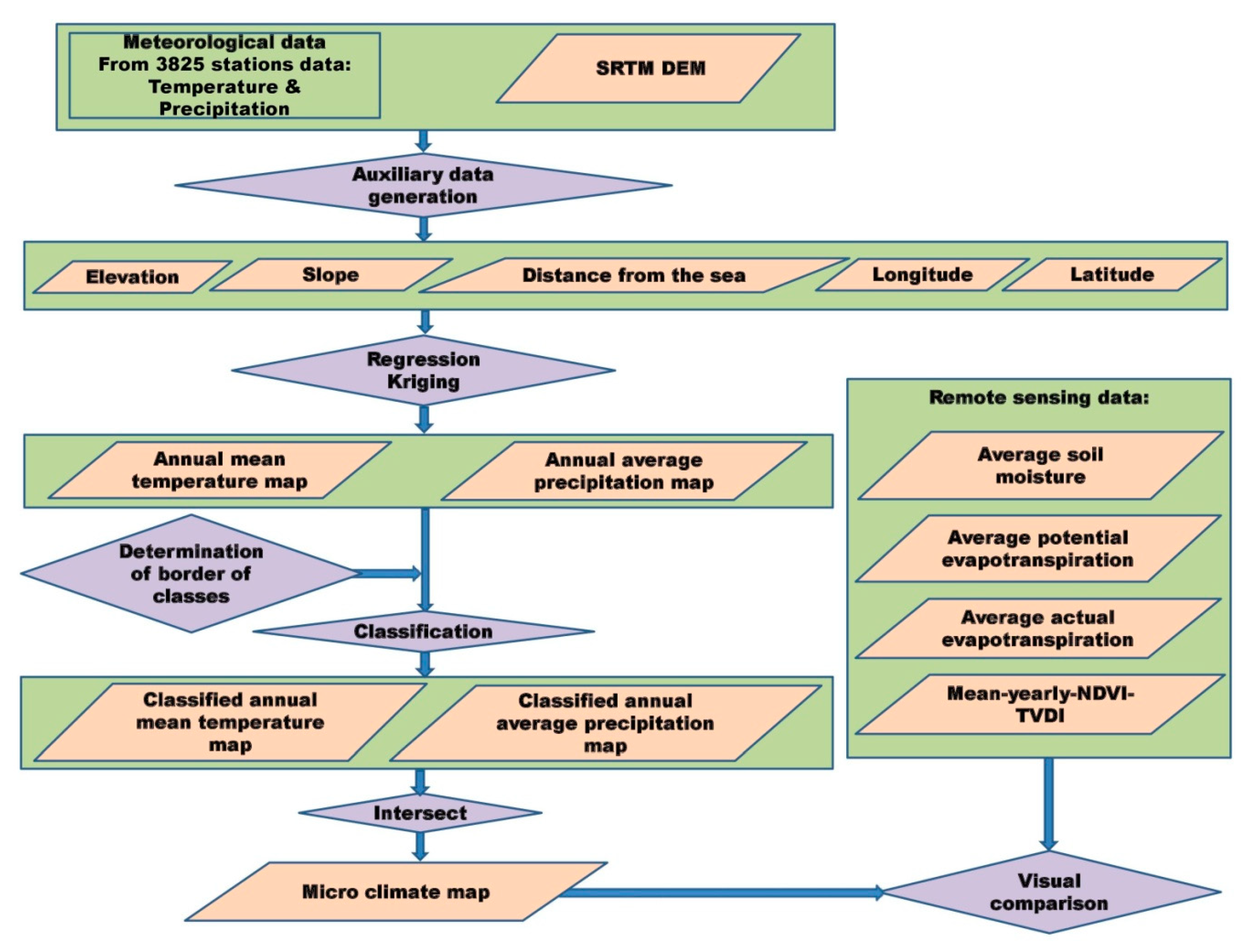
2. Materials and Methods

The methodology of the study is illustrated in Figure 1.

2.1. Description of the Study Area

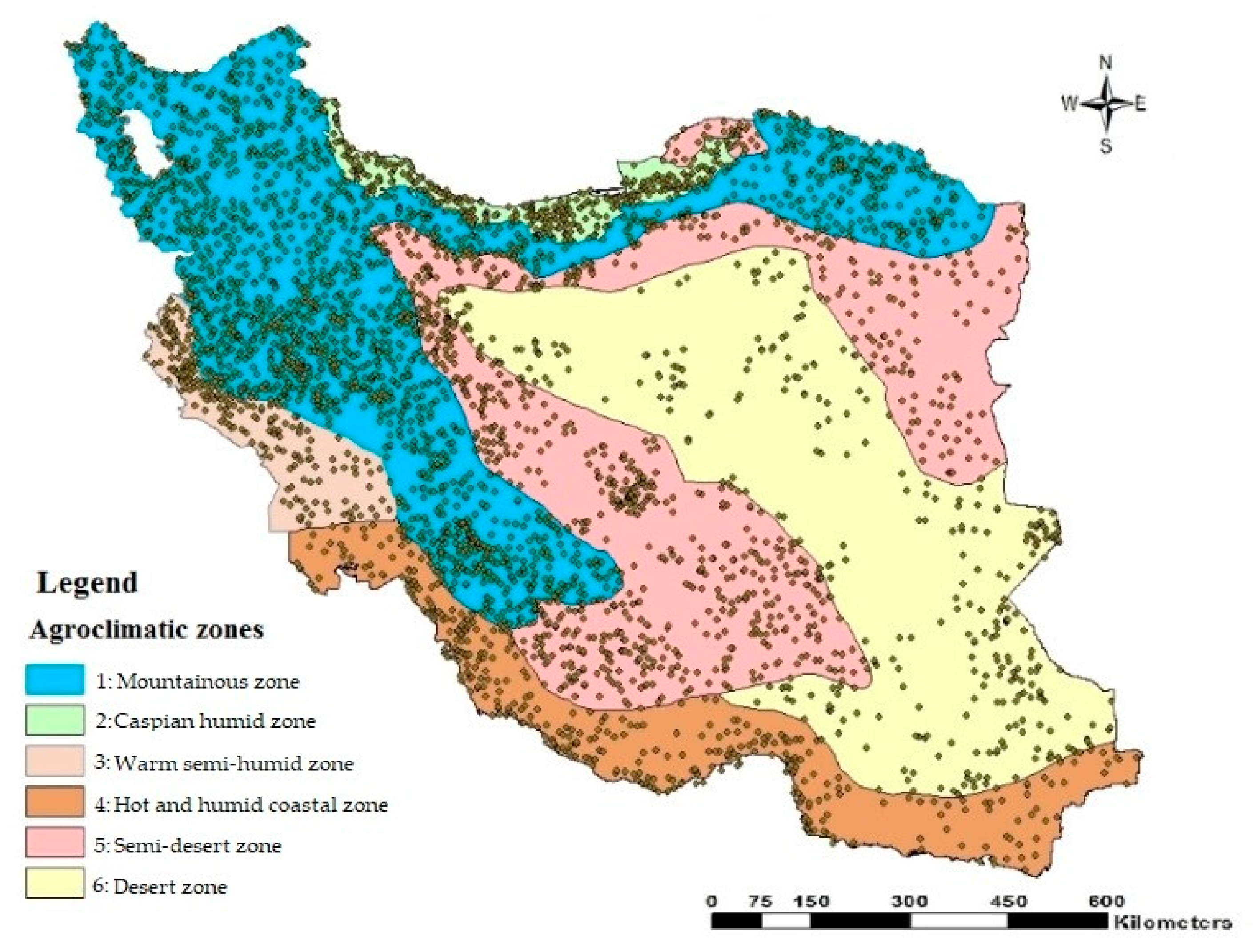
Iran, with an area of 1,648,195 km², is located in the arid belt of the Eastern Hemisphere, in West Asia, between the northern latitudes of 25–45° and the eastern longitudes of 44–63°. The country borders the Caspian Sea in the north and the Persian Gulf and Oman Sea in the south. Two ranges of high mountains, the Alborz in the north and the Zagros in the west, have a vital role in preventing the Mediterranean and the Caspian Sea winds near the central plateau of Iran. Based on atmospheric pressure, Iran is located in a low-pressure area, and accordingly, air currents form in the north and the northwest regions. The country has a variable climate. It is mild and quite wet on the coast of the Caspian Sea, continental and arid on the plateau, cold in the high mountains, and hot on the southern coast and in the southeastern region. The weather conditions of Iran are controlled by various factors. The relatively constant weather features in different regions of Iran have been formed because of different latitudes, reliefs, and proximity to large water bodies. The variable features are, however, influenced by the performances of atmospheric systems. Iran Meteorological Organization presented an agro-climatic classification for the country to organize and update the agricultural meteorological activities. In this classification, based on the major meteorological and agricultural characteristics of different areas, Iran was divided into six agro-climatic zones, including (1) the mountainous zone, (2) the Caspian humid zone, (3) the warm semi-humid zone, (4) the hot and humid coastal zone, (5) the semi-desert zone, and (6) the desert zone [27]. This agro-climatic zoning was used as the basis for the initial division in this study (desert zone, Figure 2).

2.2. Meteorological Data

Annual mean temperature and annual average precipitation data were calculated using data that were recorded from 2002 to 2016 at 185 synoptic stations and 3400 hydrometric stations from Iran Meteorological Organization (IRIMO) and 240 evaporation stations from the Ministry for Energy, which were used after being analyzed by the cumulative deviation test and quality control (Figure 2). The annual mean temperature is calculated by averaging the whole period of daily temperature averages, and the annual average precipitation is calculated by averaging the annual summation of the daily precipitation data for each year.

2.3. Auxiliary Data

At first, using NASA’s Shuttle Radar Topography Mission (SRTM) instrument in a 90 m × 90 m raster network, the digital elevation model (DEM) was produced. Then, in ArcMap (Arc GIS 10.30 software, Redlands, CA, USA), slopes derived from DEM and two separate raster layers for longitude and latitude were generated with the same extent and resolution to be used. In addition, a raster of distance from water bodies was generated with the Euclidian Distance tool using the sea boundary shapefile in ArcMap. Then, the values of these rasters were extracted for all stations.

2.4. Remote Sensing Data

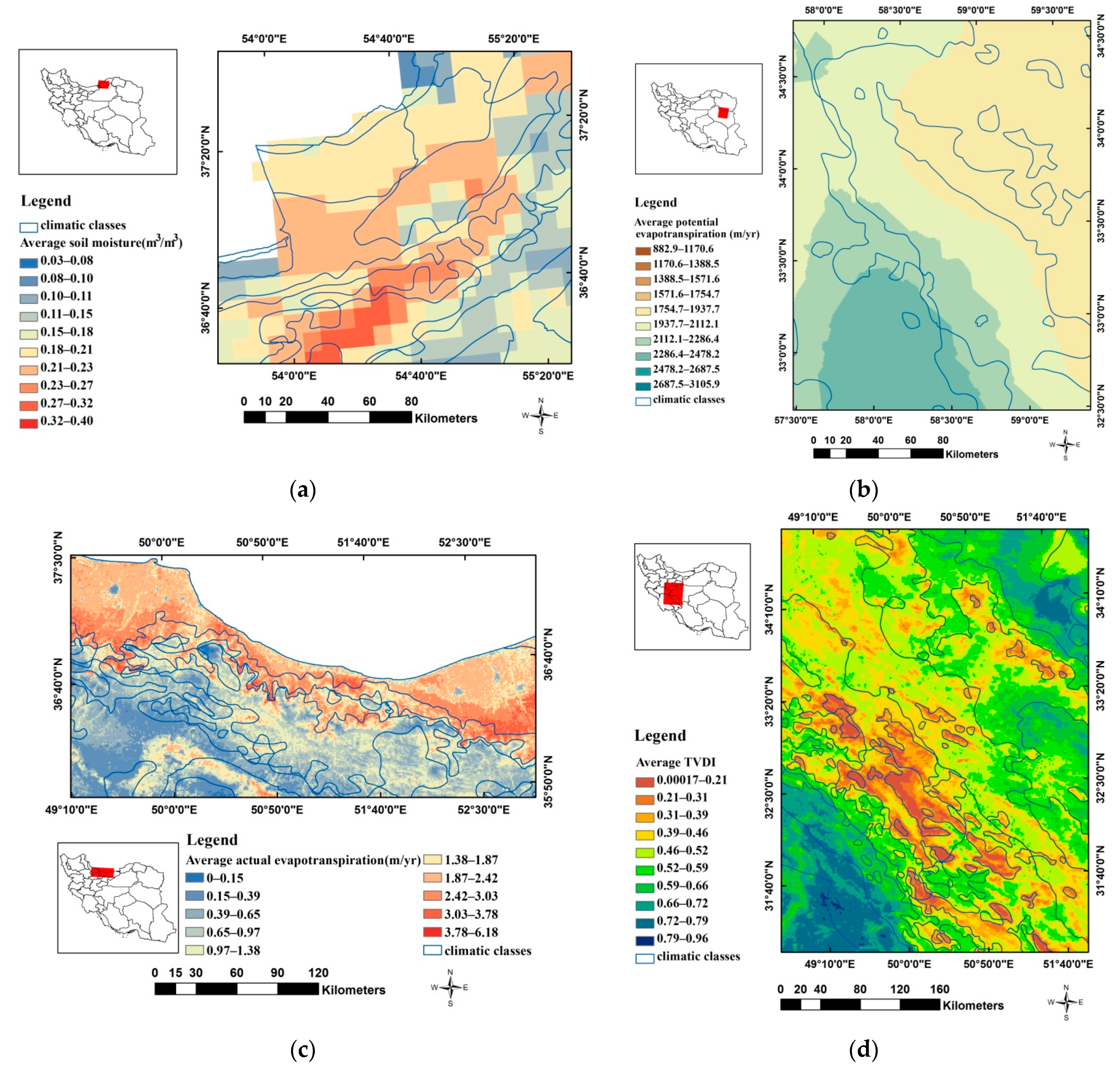
Four raster maps related to remotely sensed agricultural-related variables were prepared: (1) the average soil moisture (m³/m³), which is related to the moisture content of 5 cm of the soil surface, for which the data of 4 SAMP satellites (statistical period from 2015 to 2021) were used. Then, to calculate it, three-hour data were intercepted, and its resolution was 9 km [28] (2). The average potential evapotranspiration (m/year), which is the annual evapotranspiration of the statistical period from 2009 to 2021 and was retrieved from the WaPORdatabase, and their average was calculated. Its resolution was 250 m (3).The average actual evapotranspiration (m/year), which is produced from the WaPORdatabase and is published by the FAO; ten-day data for the statistical period from 2009 to 2021 were downloaded, and the average statistical period was calculated. Its resolution was 250 m [29] (4). The mean yearly TVDI (Temperature Vegetation Dryness Index) is one of the agricultural drought indexes and is calculated based on the NDVI and land surface temperature. Its resolution was1 km [30]. Each of the components was downloaded from the MODIS satellite for a statistical period from 2000 to 2021; then, the index was calculated for each year, and finally, the total average for 22 years was calculated.

2.5. Descriptive Statistics

The minimum, maximum, average, median, standard deviation, skewness, kurtosis, and the coefficient of variation (CV) of the annual average precipitation and annual mean temperature data were determined. The normal frequency distribution of the studied variables was evaluated by the skewness and kurtosis significance tests. The CV was classified according to CV ≤ Md − Ps, Md − Ps < CV ≤ Md + Ps, and CV > Md + Ps, respectively, representing the low, moderate, and high classes where Md and Ps, respectively, represent the median and the pseudo sigma standard deviation, where the latter can be written as:

$$\mathrm{PS}=\frac{Q3-Q1}{1/35}$$

(1)

where Q1 and Q3 denote the first and third quartiles, respectively [31].

2.6. Regression-Kriging

Regression-kriging is a hybrid geostatistical method that combines multiple linear regression between the target variable and secondary parameters with geostatistical methods, such as ordinary kriging or simple kriging, on the residuals of the regression. This method is done to optimize the prediction of the target variable in unsampled locations [13] based on the assumption that the deterministic component of the target variable is accounted for by the regression model, while the model residuals represent the spatially varying but dependent component [32].

SPSS software was used for statistical and regression analysis. To achieve greater comprehensiveness and to determine more significant variables in each agro-climatic zone, a stepwise regression method was used to develop multivariate linear regression. In this method, the linear correlation of variables was first determined, and after entering a new variable, variables that decreased their significance when adding other variables were excluded. The accuracy of the regression fitting was evaluated using the adjusted coefficient determination (R²a).

To reduce the temperature extrapolation error (as much as possible), a 10-km buffer was created around each agro-climatic zone, and the stations located in the buffer were also involved in the interpolation of the relevant zone. The equations obtained in each zone were applied to the whole zone and the surrounding buffer, and finally, by merging the zones and averaging the buffer zones, a particular thematic map was created for the whole country.

The independent variables were the digital elevation model (DEM) components, including the latitude (UTM), longitude (UTM), elevation (m), slope (%), and distance from the sea border (m), for all the stations. The dependent variables included the annual mean temperature and the annual average precipitation.

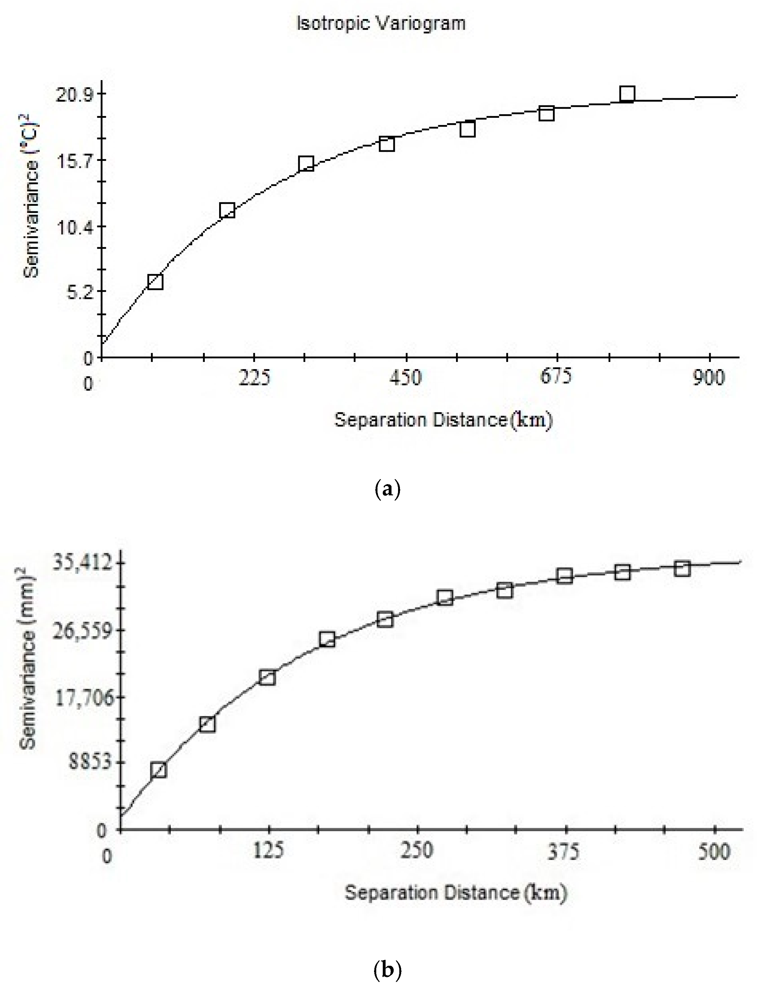
2.7. Geostatistics and Mapping

The climate zones were identified in various geographical environments by the simultaneous use of data processing techniques and tools employed in spatial data analyses and geographical studies.

To evaluate the spatial structure, variables lacking a normal frequency distribution were first normalized by logarithmic transformation. The spatial structure was then evaluated using the experimental semi-variogram. The values obtained from the experimental semi-variogram were fitted to spherical, exponential, linear, and nugget effect (C0) semi-variogram models. The coefficient of determination (R²) and the residual sum of squares (RSS) were used to evaluate the accuracy of the fitted model. Each semi-variogram consists of three components, namely the nugget effect, sill (C0 + C1), and the range. To determine the size and intensity of the spatial structure, the Cambardella Index (Ic) was used, which is the ratio of the nugget to the sill and indicates how the dataset is spatially arranged. Thus, Ic less than 25 show a strong spatial dependence and small erratic variance, while Ic between 25 and 75 show a moderate spatial dependence, and Ic greater than 75 demonstrate random spatial distribution [33]. Additionally, the mean correlation distance (MCD) was used to calculate the distance in which a high spatial dependence occurred in the variogram. In fact, the MCD is an empirical index that provides some indication of the spatial structure [34], and it was originally derived for soil properties. The greater the MCD, the greater the spatial structure [35]. The index can be written as:

$$MCD=\frac{3}{8}\left(\frac{C}{C0+C}\right)\ast a \mathrm{for} \mathrm{a} \mathrm{spherical} \mathrm{model}$$

(2)

$$MCD=\left(1-e^{-3}\right)\frac{aC}{3\left(C0+C\right)} \mathrm{for} \mathrm{an} \mathrm{exponential} \mathrm{model}$$

(3)

where C0 is the nugget, C is the partial sill, C0 + C is the total sill, and a is the range. The nugget effect represents random nonsystematic variations, and the spatial dependence decreases as its contribution to the total variations increases. The range is a distance at which variables have spatial similarity and dependence. MCD is an empirical index that provides some indication of the spatial structure.

Regression-kriging was used for zoning the spatial distribution of the parameters. It is a hybrid method that combines two approaches; that is, regression is used to fit the explanatory variation, and ordinary kriging, with an expected value of 0, is used to fit the residuals, i.e., unexplained variations [36]. The mean bias error (MBE), the mean absolute error (MAE), and the normalized root mean square error (NRMSE) were used to evaluate the accuracy of the interpolations. These three indicators can be written, respectively, as

$$MBE=\frac{{{\displaystyle \sum }}_{i=1}^n\left(P_i-O_i\right)}{n}$$

(4)

$$MAE=\frac{{{\displaystyle \sum }}_{i=1}^n\left|P_i-O_i\right|}{n}$$

(5)

$$NRMSE=\frac{100}{\overline{O}}\times \sqrt{\frac{{{\displaystyle \sum }}_{i=1}^n{\left(O_i-P_i\right)}^2}{n}}$$

(6)

where O_i is the observed value, P_i is the predicted value, $\overline{O}$ is the mean of the observed values, and n is the number of observations. The MBE is used to estimate the average bias in the model, and the closer it is to 0, the lower the bias is. Its positive values represent overestimations, and its negative values indicate underestimations. The MAE is one of the best overall measures for evaluating the agreement between observed and predicted data [37], and when it shifts to zero, the applied method simulates this fact well [38]. Moreover, a simulation is considered excellent if its NRMSE is less than 10%, good if it is greater than 10% and less than 20%, fair if it is greater than 20% and less than 30%, and poor if it is greater than 30% [39]. Based on the best interpolation method for the annual average precipitation and the annual mean temperature, the spatial distribution of the different parameters was generated for the whole country. The spatial patterns of data and fitting of the semi-variogram models were analyzed using geostatistical software GS+ version 5.1 for Windows (Gamma design, Inc., 2000, Cambridge, MA, USA). Then, Arc GIS 10.3 was employed for the interpolation methods and preparation of the annual mean temperature and annual average precipitation maps.

2.8. Classification of Produced Maps and Preparation of Climatic Maps

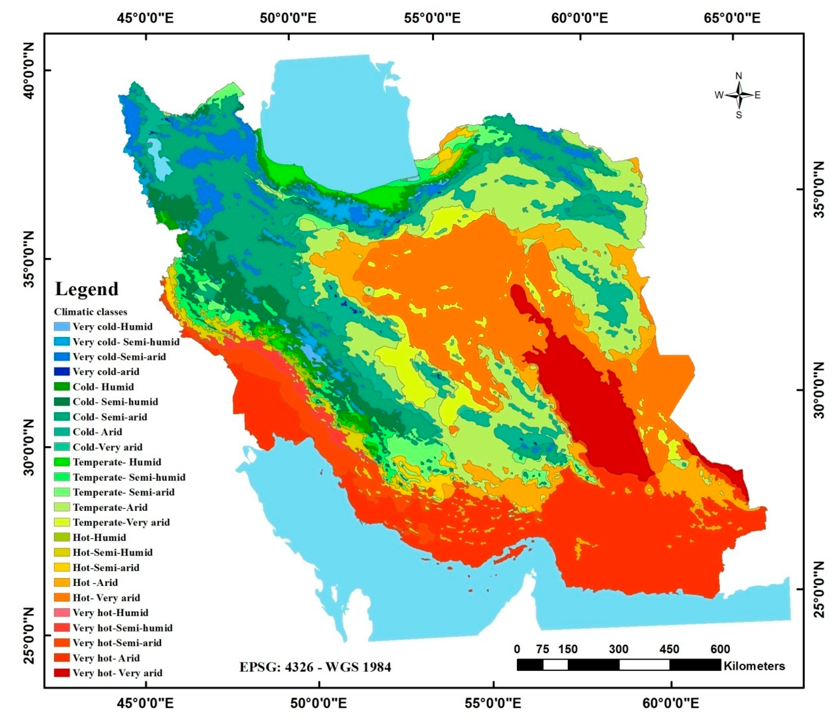
A great challenge facing climate classification is to delineate the borders of temperature and precipitation classes because of the continuous nature of both parameters. Additionally, every parameter should be classified in such a way that the classes generated in combination with other classes lead to significant classes. The use of mathematical and statistical indices such as quartiles in determining the classes of each parameter may lead to insignificant climate classes, which are uninterpretable. Therefore, the borders of the precipitation and temperature classes were determined and delineated in meetings with IRIMO and the Iran Ministry of Agriculture experts. Then, the classified temperature and precipitation were sent to the selected synoptic stations to receive the experts’ opinions and assessments regarding the accuracy and consistency between the map outputs and the local data, as well as some ecological items such as vegetation patterns using Google Earth or some available maps.

In the next step, using intersect tool in ArcMap, the two final classified maps (annual mean temperature and annual average precipitation) were overlayed to obtain a climatic map. To check the accuracy of the map, experts’ opinions were used.

2.9. Significance and Application of the Generated Climatic Map

Since a detailed quantitative comparison is beyond the objective of this study, just four raster maps related to remotely sensed agricultural-related variables, including the average soil moisture (m³/m³), average potential evapotranspiration (m/year), average actual evapotranspiration (m/year), and mean yearly TVDI (Temperature Vegetation Dryness Index), were visually compared with the generated climatic map to have a look at the qualitative significance of the generated map for future forthcoming studies.

3. Results

3.1. Descriptive Statistics

Table 1. Descriptive statistics of the annual mean temperature and annual average precipitation of Iran from 2002 to 2016.

Variable	Minimum	Maximum	Range	Mean	Quartile1	Median	Quartile3	Standard Deviation	Skewness	Kurtosis	CV (%)
annual mean temperature (°C)	1.5	30.9	29.4	19.2	16	18.4	23.5	5.2	−0.78	−0.48	27
Annual average precipitation (mm)	30.1	1580	1549.9	252.6	111	190.1	325.3	204.3	2.11	6.11	81

shows the descriptive statistics, including the annual mean temperature and the annual average precipitation, for the whole of Iran for the 15-year period.

The mean and the median annual temperatures in Iran are, respectively, 18.4 and 19.2 °C. In addition, the CV of the annual mean temperature (27%) based on the classification proposed by [31] is large.

The annual average precipitation in Iran equals 329 mm. The minimum precipitation in desert regions is 50 mm, which reduces even to zero in some years. The maximum annual precipitation over 1500 mm is observed in Bandar Anzali City, near the Caspian Sea, in the north of Iran.

3.2. Spatial Dependence

The optimum semi-variogram models fitted to the studied variables are shown in Figure 3, and their components are presented in

Table 2. Components of the best optimum semi-variogram model fitted to the two studied variables.

Variable	Model	Range (km)	Nugget Effect	Sill	Nugget effect/Sill (%)	MCD (km)	R2	RSS
Annual mean temperature (°C)	Exponential	258	0.85	21.2400	4.001	78.45	0.991	1.43
Annual average precipitation (mm)	Exponential	162	1400	37,040	3.78	49.37	0.998	1.22 × 106

. Both parameters follow the exponential semi-variogram model. The range indicates the distance at which the variable has spatial dependence.

According to Cambardella classification [33], both variables showed a strong spatial dependence, with a spatial dependence ratio (nugget effect to sill) equal to or less than 25%. Besides, MCD was used to consider the role of the range in the strength of the spatial structure.

3.3. Relationship of Annual Mean Temperature to Geographical Coordinates Components

Table 3. Relationship between the annual mean temperature and the components of the geographical coordinates in six agro-climatic zones.

Agro-Climatic Zones	Suggested Equation	R2a	RMSE	p-Value
Zone 1	T = 57.8 − 0.9949y − 0.005664h	0.76	1.56	<0.01
Zone 2	T = −8.0 + 0.4866x − 0.0043h	0.9	0.54	<0.01
Zone 3	T = −39.9 + 1.375x − 0.00545h	0.92	1.37	<0.01
Zone 4	T = 32.5 − 0.1935y − 0.00279h	0.48	1.05	<0.01
Zone 5	T = 62.9 − 0.131x − 0.905y − 0.00578h	0.77	1.38	<0.01
Zone 6	T = 49.8 − 0.7192y − 0.0054h	0.88	1.01	<0.01

T: annual mean temperature, x: longitude, y: latitude, and h: elevation of the meteorological stations considered.

shows the results of the stepwise multivariate regression fitting and the relationship between the annual mean temperature and DEM components for different agro-climatic zones. In fact, after using the stepwise method, from the DEM components, only the elevation remained in the equation. As seen, the temperature decreases with the increasing elevation and latitude.

Given the large range (107,946 m), the annual average precipitation in most regions exceeded the agro-climatic borders. No significant correlation was obtained separately for each region. However, the annual average precipitation in Iran was correlated with the latitude, longitude, and elevation of the meteorological stations:

$$P=638-15.53x+17.30y-0.0626h$$

(7)

R²a = 0.45

where p represents the annual average precipitation, x the longitude, y the latitude, and h the elevation.

3.4. Validation of Interpolation Methods

Evaluations of the interpolation accuracy of the annual mean temperature and the annual average precipitation are shown in

Table 4. Statistical indicators for validation of the interpolation methods for the annual mean temperature and annual average precipitation.

Statistical Index	Annual Mean Temperature	Annual Average Precipitation
MBE	−0.05	0.69
MAE	0.93	0.76
NRMSE	6.41	9.18

. In regression-kriging, for both target variables, the longitude, latitude, and elevation ofthe meteorological stations were used as auxiliary variables. Significant relationships between the auxiliary variables and target variables caused good MBE, MAE, and NRMSE for the predictions of both the annual mean temperature and annual average precipitation. The NRMSE was less than 10% for the two interpolated variables.

The annual mean temperature and the annual average precipitation obtained from regression-kriging aredisplayed in Figure 4 and Figure 5. The maps were prepared with a resolution of 5 km.

According to the spatial distribution of the variables, on the one hand, the annual mean temperature decreases from south to north and from east to west, and on the other hand, the mean temperature in the mountainous regions, such as the Zagros and the Alborz Mountains, is lower than that over the plain areas (Figure 4a). The temperature decline from east to west and from south to north is mainly due to the Zagros Mountains and the movement of the Siberian air masses towards the central desert of Iran. The lowest temperature was observed in Northwest Iran and over the Zagros Mountains. In contrast, the highest temperature was seen in the Oman Sea coastal region and the Strait of Hormoz. The temperature decreases from the southeast to the northwest and west of Iran, which correspond to very high altitudes. Consistent with the mountainous regions but with lower elevations than the very cold regions, most regions are cold from the southeast to the southwest and west of Iran. Temperate temperatures are observed in some regions of the east, the Caspian zone, center, and west of Iran. Some regions of Central and Eastern Iran correspond to the hot temperature class. These regions are mainly consistent with the desert areas and the Sistan Plain in Southeastern Iran. The southeastern areas and southern and southwestern coastlines are very hot (Figure 4b).

The evaluation of the spatial distribution of the annual average precipitation showed that the higher precipitation values are concentrated on the Caspian coastlines in the north and western hillsides of the middle of the Zagros, followed by other regions along the Alborz and the Zagros hillsides. The central and southeastern areas are among the regions with the lowest precipitation in Iran. A low-precipitation core is observed in the central deserts of Iran, with three high-precipitation cores in the Zagros (Figure 5a).

The eastern regions towards Central Iran are areas with very low precipitation (very arid), and precipitation is still much lower in the southeastern regions towards the southern coasts of Iran (arid). The southeastern regions towards the west and the southwest matching the Alborz and the Zagros foothills are semi-arid, and high-altitude regions with higher precipitation rates correspond to the semi-humid class. The high-precipitation (most humid) areas are located along the Caspian Sea coasts and some regions in the west of Iran (Kuhrang) (Figure 5b).

The annual mean temperature and annual average precipitation base maps were used for climate zoning (Figure 4 and Figure 5). Based on the IRIMO and the Iran Ministry of Agriculture’s expert opinions, the borders were determined, and each map was classified into five classes, representing certain precipitation or temperature situation. The temperature classes included very cold (<10 °C), cold (10.1–15 °C), temperate (15.1–18.5 °C), hot (18.6–22 °C), and very hot (>22.1 °C) areas. The precipitation classes also included very arid (<100 mm), arid (100.1–250 mm), semi-arid (250.1–400 mm), semi-humid (400.1–700 mm), and humid (>700.1 mm) areas. By combining these classes, 24 temperature–precipitation classes were then obtained.

The different climate classes obtained by combining the precipitation and temperature classes are shown in Figure 6, and the properties of the climatic classes in terms of the annual average precipitation, annual mean temperature, and elevation are listed in

Table 5. Characteristics of Iran’s climatic classes.

Climatic Classes	Annual Average Precipitation (mm)	Precipitation Classes	Annual Mean Temperature (°C)	Temperature Classes	Minimum Elevation (mm)	Maximum Elevation (m)	Median of Elevation (mm)	Area (km2)	Relative Area (%)
Very hot Arid	100.1–250	Arid	>22.1	Very hot	−82	2115	1020.5	266,769.3	16.47
Hot very arid	< 100	Very arid	18.6–22	Hot	433	2316	1349	232,878.5	14.38
Temperate Arid	100.1–250	Arid	15.1–18.5	Temperate	−50	4107	1950.5	215,553.7	13.31
Cold semi-arid	250.1–400	Semi-arid	10.1–15	Cold	205	3874	2016	183,679.1	11.34
Cold Arid	100.1–250	Arid	10.1–15	Cold	528	4209	2450	102,490.3	6.33
Hot Arid	100.1–250	Arid	18.6–22	Hot	3	3113	1492	98,980.1	6.11
Very hot Very arid	<100	Very arid	>22	Very hot	105	1502	800.5	81,956.5	5.060
Cold Semi-humid	400.1–700	Semi-humid	10.1–15	Cold	291	3662	1949	71,112.0	4.39
Temperate Very arid	<100	Very arid	15.1–18.5	Temperate	768	2868	1800.5	55,103.5	3.40
Very cold Semi-arid	250.1–400	Semi-arid	<10	Very cold	1091	5597	3212.5	53,710.2	3.32
Very hot Semi-arid	250.1–400	Semi-arid	>22	Very hot	−49	2225	1070	45,550.9	2.81
Temperate Semi-arid	250.1–400	Semi-arid	15.1–18.5	Temperate	−72	3534	1753	42,982.1	2.65
Temperate Semi-humid	400.1–700	Semi-humid	15.1–18.5	Temperate	−297	3487	1702.5	29,567.0	1.83
Very cold Semi-humid	400.1–700	Semi-humid	<10	Very cold	939	4794	2861	23,290.5	1.44
Temperate Humid	>700.1	Humid	15.1–18.5	Temperate	−90	2915	1397	23,016.1	1.42
Cold Humid	>700.1	Humid	10.1–15	Cold	24	3514	1752.5	22,505.8	1.39
Hot Semi-arid	250.1–400	Semi-arid	18.6–22	Hot	−14	3065	1497.5	20,080.9	1.24
Hot Semi-Humid	400.1–700	Semi-humid	18.6–22	Hot	−25	2780	1381	19,904.6	1.23
Very hot Semi-humid	400.1–700	Semi-humid	>22	Very hot	30	1914	954	15,974.1	0.99
Very cold Humid	>700.1	Humid	<10	Very cold	413	4178	2303.5	5825.0	0.36
Hot Humid	>700.1	Humid	18.6–22	Hot	34	2520	1232.5	4808.3	0.30
Cold Very arid	<100	Very arid	10.1–15	Cold	1352	3138	2231	2568.3	0.16
Very cold arid	100.1–250	Arid	<10	Very cold	1513	4042	2765.5	1352.6	0.084
Very hot Humid	>700.1	Humid	>22.1	Very Hot	355	1242	801	171.04	0.011

. The largest climate class area in Iran is the very hot arid class, followed by the hot very arid regions. The annual precipitation in these two classes is 100–250 mm and less than 100 mm, respectively. The corresponding mean temperature is above 22 °C and 18–22 °C, respectively. These two classes cover around 31% of Iran’s mainland. The hot arid climate classes mainly extend into the non-mountainous regions, including deserts and the southern and southeastern margins. These climate classes often have lower minimum and median elevations than other climate classes. The very cold humid to semi-arid climate classes cover the smallest area of Iran as a mosaic in the Alborz and the Zagros Mountains with higher minimum and median elevations. The temperate arid class showed the highest frequency among the moderate classes, which is extended to the southern margin of the Alborz Mountain chains and the eastern margin of the Zagros Mountain chain.

3.5. Significance and Application of the Generated Map

A visual comparison showed that there was a sort of agreement between the produced climate map and the remote sensing agricultural variable (Figure A1).

4. Discussion

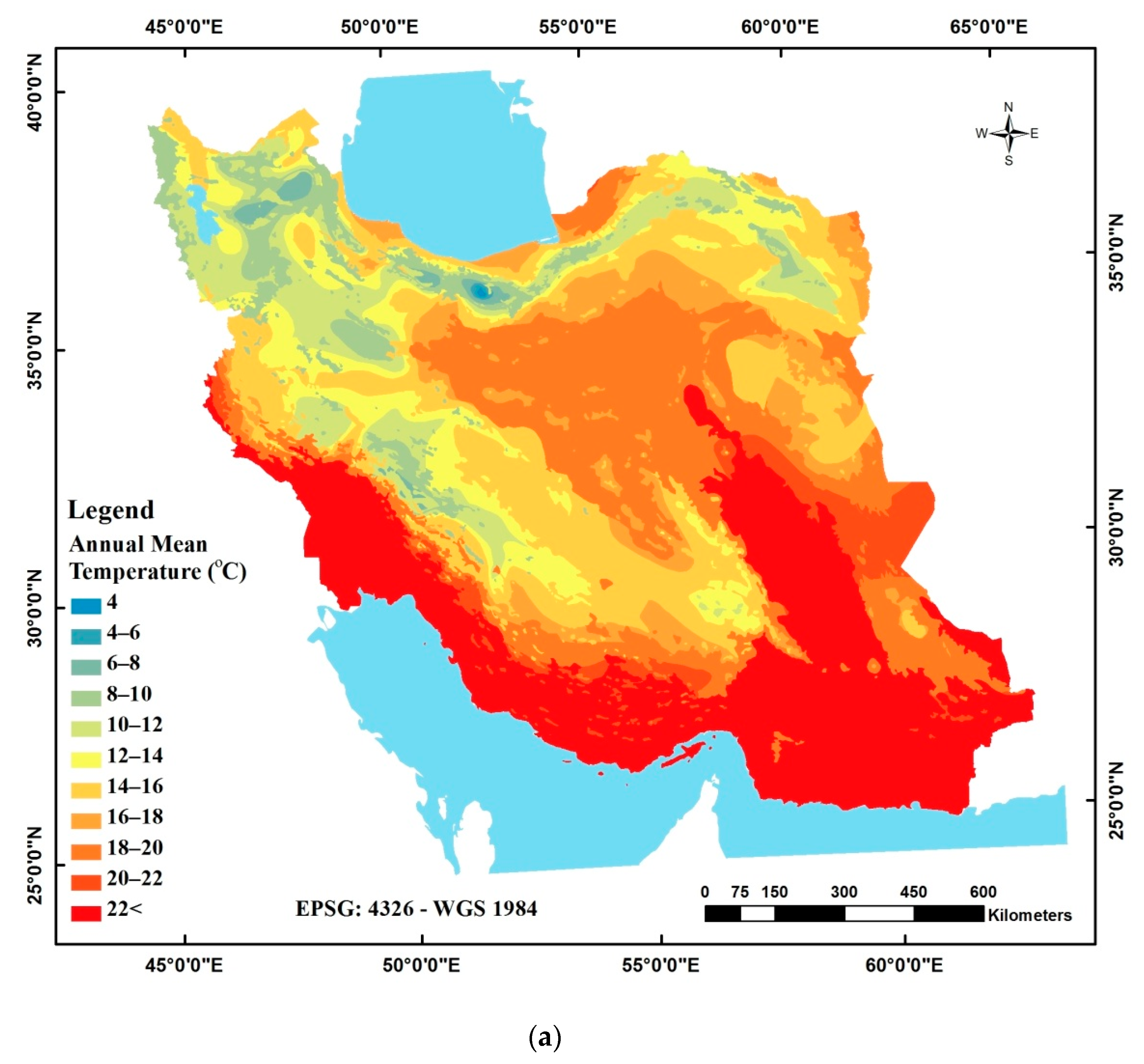
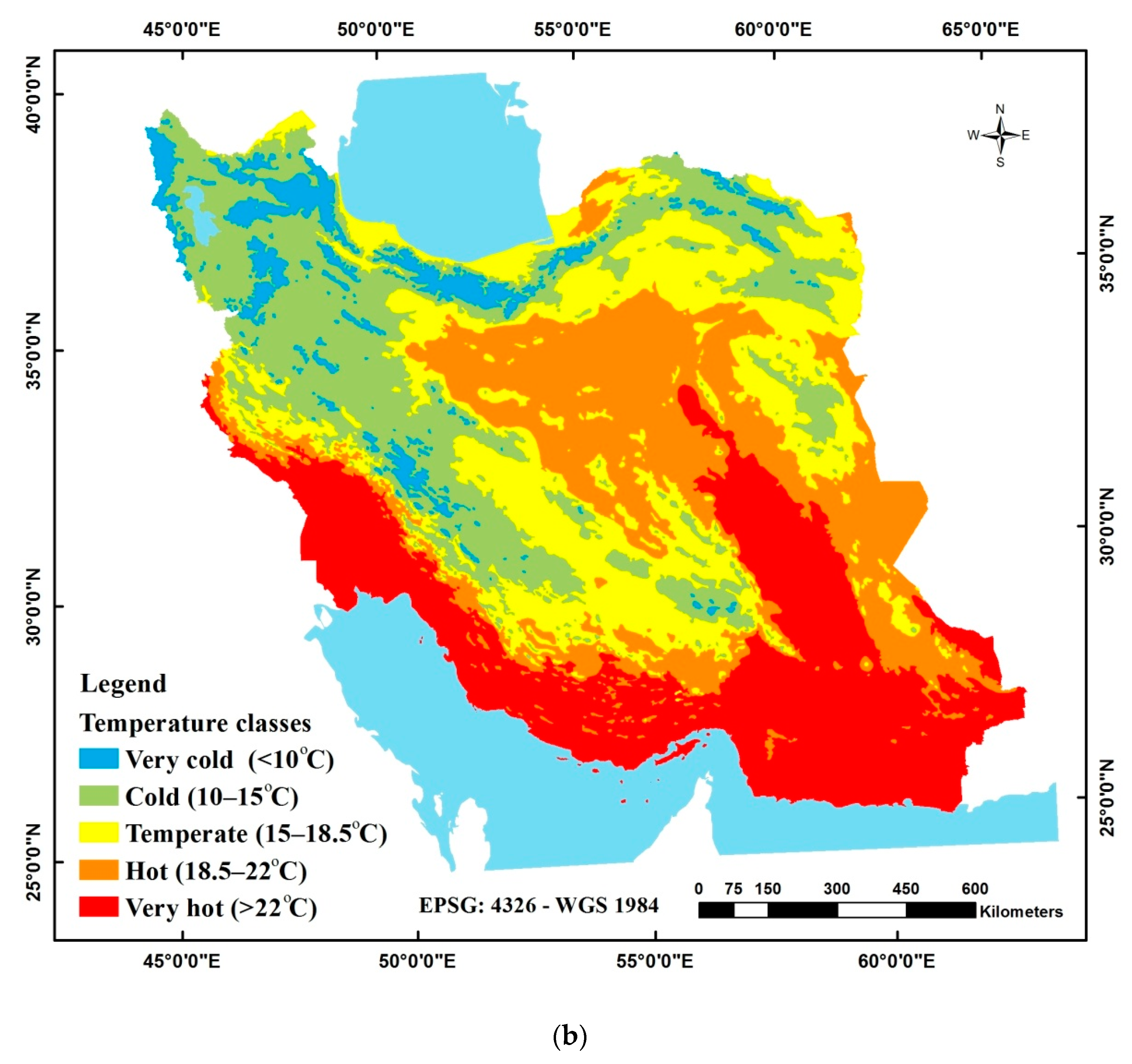
The large nonuniformity of the annual mean temperature is expected due to the vastness of Iran, large elevation variations, and proximity to the Persian Gulf and Oman Sea in the south and the Caspian Sea in the north.

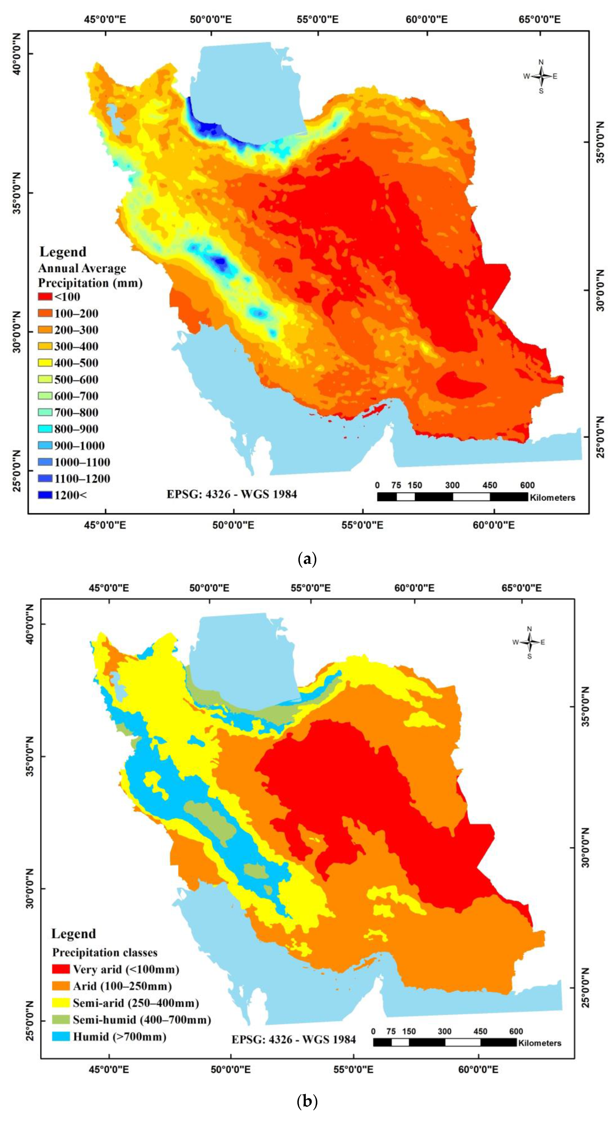
The annual average precipitation is a function of latitude and elevation. The maximum annual precipitation is mainly observed near the Caspian Sea in the north of Iran. Considering Equation (7), it can be concluded that relief plays a key role in the arrangement of different precipitation classes in Iran. The annual temperature increases by 2.6 °C from west to east per 10,000 km, whereas the temperature increases by 7.8 °C from north to south. However, increases in elevation have different impacts on precipitation. Precipitation usually increases as the elevation increases up to a certain amount, decreasing afterward. Furthermore, a change in the latitude of different regions may cause a change in the precipitation rate due to permanent rotation cycles of the atmosphere [40]. According to the calculated equation, precipitation increases with the increasing latitude, which is relatively connected to Iran’s topography. The precipitation system influencing Iran from the Mediterranean Sea causes the maximum precipitation in the Zagros Mountains, which gradually decreases with the increasing longitude towards the center and east of Iran. Precipitation also increases with the increasing elevation, except for the Caspian Sea coastline, with a negative elevation below the sea level, the zone that is rainier than other regions due to specific climatic and topographic conditions. Lower precipitation rates are usually recorded at the stations located at positive elevations above the sea level in other regions. The combination of these two factors leads to a negative regression coefficient with increasing elevation.

According to the semi-variogram model fitted to the studied variables, the annual mean temperature showed more spatial dependency than the annual average precipitation. It may be assumed that the decrease in spatial dependency in the annual average precipitation is due to the nonuniform topography, and most parts of the western and northern areas are more affected by the Mediterranean humid air masses than the central, eastern, and southern areas of Iran. Based on Cambardella classification [33] and MCD, the annual mean temperature showed a higher spatial dependency at larger distances.

The results of the stepwise multivariate regression fitting showed that the annual mean temperature follows the geographical coordinates and height in six agro-climatic zones. In fact, the temperature decreases with the increasing elevation and latitude. The changes in the atmospheric parameters, including temperature and precipitation, are consistent with the variations in the spatial and topographical characteristics. The lapse rate, the rate at which the temperature changes with the height in the atmosphere, is an indicator of the direct impact of elevation on the temperature. Due to the effect on the angle of solar radiation, the latitude causes a change in the temperatures of different regions. The air temperature decreases from east to west and from south to north. Latitude plays a much more significant role than longitude in the spatial variability of the temperature across Iran.

The generated map for the annual mean temperature is highly consistent with a previous study by Aliabadi and Roudbari [12], in which the combination of the spatial statistics methods and autocorrelation indices demonstrated a negative spatial autocorrelation of the maximum temperature (low-value temperature clusters) on the Caspian Sea coastline and the west, northwest, and southeast of Iran. In contrast, some regions in the center and southwest of Iran showed a positive spatial autocorrelation (high-value temperature clusters) [12]. Accordingly, most mountainous regions and highlands in Iran are dominated by lower temperature values. However, the southeast and southwest of Iran show the maximum temperature due to high humidity, and the Dasht-e Lut and Dasht-e Kavir with poor cloudiness.

The resulting zoning for precipitation is very similar to that reported by Doostkamian and Mirmousavi [24], who divided Iran into four regions according to precipitation thresholds.

Comparisons of the existing maps from previous studies such as Heidari and Alijani [21] and Ghaffari and Ghasemi [23] in Iran showed that the newly generated map has acceptable and more realistic classes thatare due to: (1) the use of the maximum data (3825 stations) to increase the spatial density of the stations and, thus, increase the spatial resolution, (2) the preparation of two temperature and precipitation rasters using the regression-kriging method, which provided a good basis for creating a microclimate map, and (3) Instead of using global thresholds, an attempt was made to use the opinions of experts to find the appropriate thresholds for classification, which resulted in the creation of more climatic classes. In fact, the 24 climate classes showed that using auxiliary variables and careful classification of the basic maps were very effective in detecting different climatic classes and, therefore, understating the climate diversity in Iran. Hot to very hot and arid to very arid climate classes were identified as the largest climatic classes of Iran, which cover Iran’s southeastern and southern desert regions. As a result, the generated map can be very beneficial for many environmental and agricultural studies, such as land evaluation studies, which consider soil and landscape characteristics and climatic parameters to suggest the most proper plant for each land to tackle the water shortage, preserve soil, and achieve sustainable agriculture.

The visual comparison of four raster maps related to remotely sensed agricultural-related variables, including average soil moisture (m³/m³), average potential evapotranspiration(m/year), average actual evapotranspiration (m/year), and meanyearly TVDI (Temperature Vegetation Dryness Index) with the generated climatic map, showed that there was a sort of agreement between these variables and the climatic generated map; thus, such high-resolution climatic maps can be a very good starting point to generate microclimatic maps, as well as it is suggested to use climatic maps to better classify, assess, and interpret remote sensing-based agricultural applications to be planned out in the close future.

5. Practical Application

Climatic information is of particular importance in any study and strategic planning of all environmental projects and the basis of many activities, especially in agriculture, animal husbandry, rangeland management, natural resources protection, and suitable cultivation pattern programs. In other words, a climatic map that is carefully classified can be a great basis for many ecological studies and decisions. It can also be used to better classify and interpret remote sensing-based agricultural rasters. As a result, the more accurate the climatic map with proper classification, the better.

The strengths of this study can be considered the generation of basic data maps (annual mean temperature and annual average precipitation) and then classification based on their thresholds in the country instead of using global ranges. Regression-kriging also helped to prepare a more accurate temperature and precipitation map. The validations showed that the prepared climatic map has acceptable accuracy. The accurate thresholds for both the annual mean temperature and the annual average precipitation resulted in a climatic map with 24 classes, which is a new and valuable achievement for the country. Therefore, it is suggested that these approaches be considered for other countries as well and not be limited to global classifications, which may result in the identification of a small number of climatic classes in a country.

6. Conclusions

In this study, using the long-term average precipitation and temperature measurements for the 2002–2016 period from 3825 meteorological stations, geographical auxiliary variables, regression-kriging, knowledge of Iran Meteorological Organization and Iran Ministry of Agriculture experts, all attempts have been made to generate new and precise maps of the temperature and precipitation for the country. Based on the CV, the annual average precipitation and the mean annual temperature, respectively, showed moderate and large variations. The generated annual mean temperature map indicated a decline in temperature from east to west and northwest in high-altitude areas, while the Caspian Sea coastline and the Zagros Mountains experienced the highestprecipitation values. By applying five delineation thresholds on the maps and intersecting the classified maps, Iran was divided into 24 climates (precipitation–temperature) zones. According to the evaluation statistics and matching generated maps with expert knowledge and some ecological items, the delineation and diversification of the climatic classes were really acceptable. According to the generated climatic map, hot to very hot and arid to very arid climate classes occupy the largest part of Iran, which are located in the southeastern and southern desert regions. The climatic diversity indicated that the regression-kriging method was useful for mapping climate zones, and the resulting map can be used for decoding natural selections andthe management of resources, especially water consumption, sustainable agricultural planning, determining the cultivation pattern, and optimizing agricultural and horticultural calendars. Furthermore, the simple visual comparison between the climatic zones from the generated climatic map and four remotely sensed agricultural variables clearly shows the usefulness of these carefully produced climatic maps for classifying, evaluating, and interpreting these and other remotely sensed agricultural-related variables and producing microclimatic maps using these types of remotely sensed variables.