Quantitative Evaluation of Grassland SOS Estimation Accuracy Based on Different MODIS-Landsat Spatio-Temporal Fusion Datasets

Abstract

Estimating the Start of Growing Season (SOS) of grassland on the global scale is an important scientific issue since it can reflect the response of the terrestrial ecosystem to environmental changes and determine the start time of grazing. However, most remote sensing data has coarse- temporal and spatial resolution, resulting in low accuracy of SOS retrieval based on remote sensing methods. In recent years, much research has focused on multi-source data fusion technology to improve the spatio-temporal resolution of remote sensing information, and to provide a feasible path for high-accuracy remote sensing inversion of SOS. Nevertheless, there is still a lack of quantitative evaluation for the accuracy of these data fusion methods in SOS estimation. Therefore, in this study, the SOS estimation accuracy is quantitatively evaluated based on the spatio-temporal fusion daily datasets through the Spatial and Temporal Adaptive Reflectance Fusion Model (STARFM) and other models in Xilinhot City, Inner Mongolia, China. The results show that: (1) the accuracy of SOS estimation based on spatio-temporal fusion daily datasets has been slightly improved, the average Root Mean Square Error (RMSE) of SOS based on 8d composite datasets is 11.1d, and the best is 9.7d ($f_{starfm}^8$); (2) the estimation accuracy based on 8d composite datasets ($\overline{RMSE}$ = 11.1d) is better than daily fusion datasets ($\overline{RMSE}$ = 18.2d); (3) the lack of the Landsat data during the SOS would decrease the quality of the fusion datasets, which ultimately reduces the accuracy of the SOS estimation. The $\overline{RMSE}$ of SOS based on all three models increases by 11.1d, and the STARFM is least affected, just increases 2.7d. The results highlight the potential of the spatio-temporal data fusion method in high-accuracy grassland SOS estimation. It also shows that the dataset fused by the STARFM algorithm and composed for 8 days is better for SOS estimation.

1. Introduction

As the most widely distributed vegetation type on the Earth, grassland covers about 4.5 billion hm², accounting for 24% of the total land area. As an important part of the terrestrial ecosystem, the grassland ecosystem which is composed of living things (plants, animals, and microorganisms) and the non-biological environment plays a critical role in material flow and energy exchange. China’s grassland ecosystem is a vital part of the temperate grassland ecosystem in Eurasia, accounting for about 1/10 of the world’s grassland area. It is essential for ecological regulation and ecological barriers.

The response of the grassland ecosystem to climate and environmental changes can be reflected by grassland vegetation monitoring, which is an important basis for grassland ecological regulation and grazing policy-making [1]. Vegetation phenology refers to the phenomenon of plants undergoing seasonal progression of activity—from germination to dormancy—associated with the changing climate during the year [2]. Additionally, grassland vegetation phenology is an essential ecological component to studying the relationship between grassland vegetation and climate and environmental changes. Furthermore, grassland vegetation changes (greening, withering) are more sensitive to climate change than woody plants [3,4,5,6]. Accurate monitoring of grassland vegetation changes can promote further research into the response degree and influence mechanism of the natural grassland ecosystem to climate change (temperature, precipitation, carbon cycle). Furthermore, the SOS is a sensitive indicator of climate change [7] and an important stage in the growth process of grassland vegetation, affecting seasonal variability in carbon, water, and energy [7,8,9,10]. Therefore, the study of grassland SOS monitoring is becoming increasingly important in vegetation phenology.

Traditional ground observation has obvious disadvantages, including the uneven distribution of ground observation stations, limited coverage, a large amount of manpower and material resources [11], and single observation species [12], which cannot meet the needs of large-scale regional monitoring for vegetation phenology. Remote sensing data is known for multi-temporal, wide-coverage, spatial continuity, and long-time series. It can be used for long-term and wide-range dynamic monitoring and trend analysis in vegetation growth [13]. A typical example is that the vegetation index of the multispectral remote sensing images can reflect the growth and changes of vegetation. Hence, remote sensing monitoring has become an effective way to reveal the response and feedback of vegetation to global climate change, which can promote the process of vegetation phenology [3,14,15,16,17,18].

At present, long time series but low spatial resolution remote sensing data (NOAA/AVHRR, SPOT VGT, MODIS) is mostly used in remote sensing vegetation SOS monitoring [9,13,14,19,20,21]. This may not only reduce the accuracy of vegetation SOS estimation but also reduce the objectivity of vegetation SOS inversion influenced by mixed pixels [22]. To reduce the impact of clouds, most researchers have used multi-day composited data, such as MODIS 16d, 10d, and 8d products [23]. In recent years, Landsat and other high spatial resolution data have gradually been applied in various related fields [24,25], but due to the disadvantages of small coverage and low frequency of revisit, it is difficult to track the seasonal change of vegetation [20,26].

Although data with higher temporal and spatial resolution can more accurately reflect vegetation growth and improve the accuracy of vegetation index reconstruction, the existing sensor technology struggles to obtain images with both high temporal resolution (or temporal frequency) and high spatial resolution [27]. Multisource remote sensing data fusion has become prevalent for improving spatio-temporal resolution [28]. It combines the advantages from two kinds of data (high spatial resolution or high temporal resolution) to generate high spatio-temporal resolution data [27,29,30,31,32,33,34,35,36,37]. Currently, many spatio-temporal fusion models have been developed, such as the Spatial and Temporal Adaptive Reflectance Fusion Model (STARFM) and the Spatial and Temporal Data Fusion Approach (STDFA). Gao et al. [27] presented STARFM for blending Landsat (high-resolution spatial information) and MODIS (high-frequency temporal information) imagery. This approach has been widely recognized in the field of vegetation phenology inversion. However, some problems include the patch effect and insensitivity to the change of heterogeneous ground objects in this algorithm. Therefore, Wu et al. [33] proposed the STDFA model to make up for the shortcomings of previous spatio-temporal fusion algorithms. After that, Xie et al. [35] proposed the Unmixing-based STARFM (USTARFM), which further solved the ‘image spot’ phenomenon in the STARFM algorithm and the difficulty in searching pure pixels. Based on the above spatio-temporal fusion results, many researchers applied it in vegetation phenology monitoring. Walker et al. [38] used STARFM to fuse Landsat and MODIS data, then constructed the 30 m daily reflectance data for dryland forest phenological inversion, and finally compared it with the inversion phenology of MODIS data. Gao et al. [39] used the Landsat and MODIS data fused by the STARFM to obtain the phenology of various crops. Compared with field observation data, the feasibility of the datasets obtained by using the spatio-temporal data fusion algorithm in crop phenology inversion was demonstrated. Onojegho et al. [40] successfully retrieved the rice phenology by using STARFM to integrate Landsat and MODIS vegetation index.

Although the spatio-temporal fusion technology has been widely used in vegetation phenology monitoring, there is still a lack of quantitative analysis about different fusion algorithms on SOS inversion. Therefore, this research used three models to fuse MODIS and Landsat data, constructed high spatio-temporal resolution (Normalized Difference Vegetation Index) NDVI data for grassland SOS inversion, and then quantitatively analyzed the SOS estimation accuracy. The goals of this study are as follows: (1) Evaluating whether spatio-temporal fusion data can improve SOS estimation accuracy compared to MODIS data; (2) Evaluating how the lack of the Landsat data during the SOS affects estimation accuracy.

2. Materials

2.1. Study Area

Figure 1 shows the study area of Xilinhot, which is located in the center of Inner Mongolia Autonomous Region, China (115°18′–117°06′E, 43°02′–44°52′N), and covers a total area of 14,785 km². The area is elevated in the south and low in the north, with an average altitude of 988.5 m. The climate in the study area is a mid-temperate semi-arid continental climate, and has annual precipitation of about 294.9 mm and a natural vegetation which is mainly grassland. The vegetation in the study area is dominated by typical grassland plants with abundant animal husbandry resources [41]. The available grassland covers an area of 13,787 km², including Warm steppes (WS), Temperate meadow-steppe (TM), Lowland meadow (LM), and Improved grassland, which has certain typicality and integrity. Therefore, the research of grassland vegetation phenology in the area is representative.

2.2. Data Resources

2.2.1. Remote Sensing Data

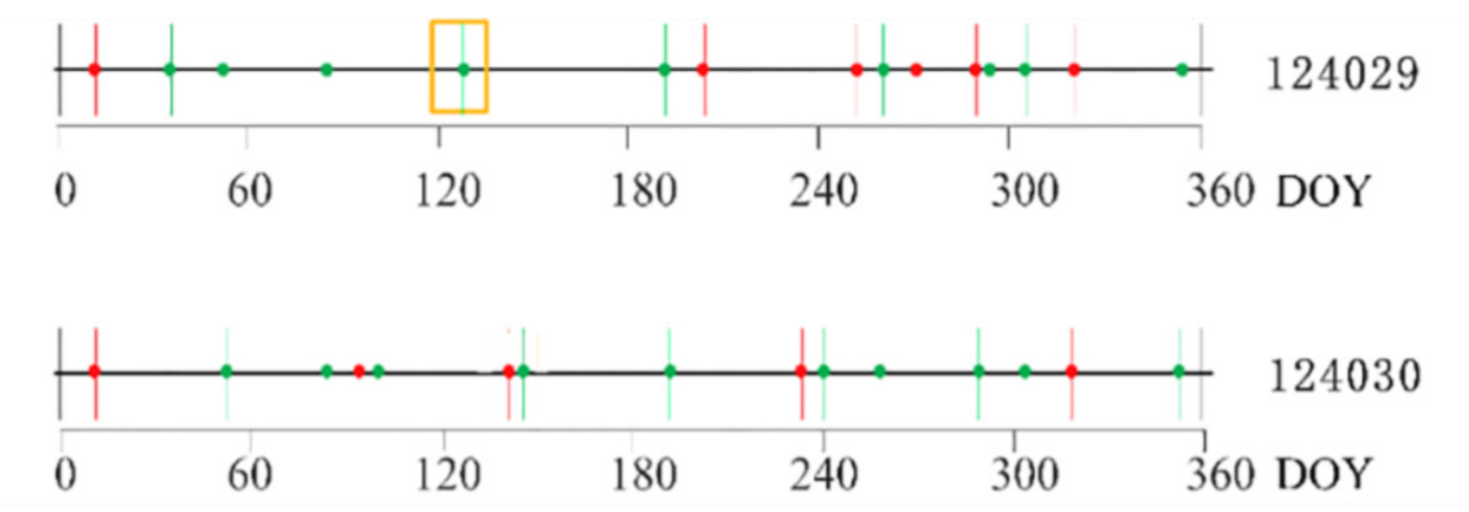
American EOS satellite MODIS MOD09GQ Level2 products (h25v03 h25v04, h26v03, h26v04) have red and near-infrared wavebands with 250 m and 1 day temporal resolution. NASA’s Landsat8 OLI Level1 products (PATH/ROW:124/029, 124/030) consist of nine bands, and the red and near-infrared bands with 30 m and 16 days temporal resolution were selected for the study. The less-cloud Landsat image (the vertical line dots in Figure 2) and the corresponding MODIS image were both selected to be the base data of Landsat-MODIS to produce the fusion images with 30 m resolution. In order to avoid the influence of clouds, we manually masked clouds for Landsat images, and MODIS images were processed with its own cloud mask data.

In this paper, radiometric calibration and atmospheric correction were carried out for the Landsat8 OLI Level1 image to obtain the real reflection image of the surface. Then, we directly used the USGS MODIS Reprojection Tool (MRT) to preprocess the MOD09GQ level 2 (represent the real reflectance of the ground surface) and converted its projection into Landsat UTM Projection (Zone 50N WGS84). In addition, for the STARFM algorithm, we used CUBIC_CONVOLUTION to resample MODIS data to obtain data with a spatial resolution of 30 m.

2.2.2. Ground Sampling Points Data

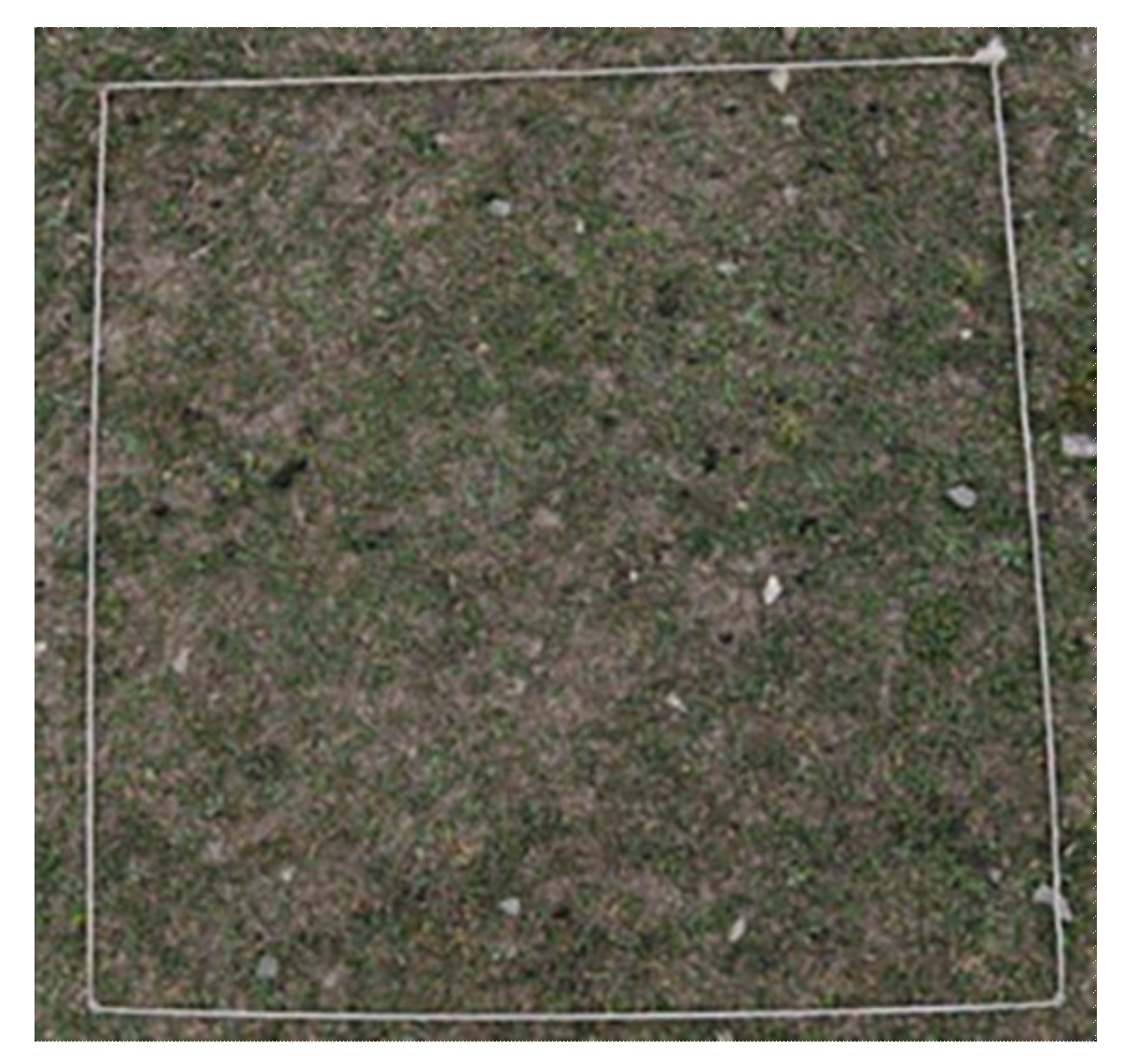
The ground sampling points (GSPs) data of Xilinhot in 2014 and 2015 were provided by the Institute of Agricultural Resources and Regional Planning, Chinese Academy of Agricultural Sciences. There were 3 sample plots and 9 GSPs in 2014, and 4 sample plots and 13 GSPs in 2015 (Figure 3). In the sample plots, each GSP should be separated by at least 250 m. The survey content mainly included sample plot number, GSP number, survey time, location, grassland type, terrain and altitude, latitude and longitude, dominant species, and SOS. As the basis of remote sensing application research, field observation plays a critical role in remote sensing modeling of vegetation phenology. The monitoring of the SOS in the field is mainly determined by the percentage of the plants (clumps) which begin to spread leaves and develop normally to the total plants (clumps) in the sample plot. The onset of SOS is indicated when the greening rate in the plot reaches 20%.

3. Methods

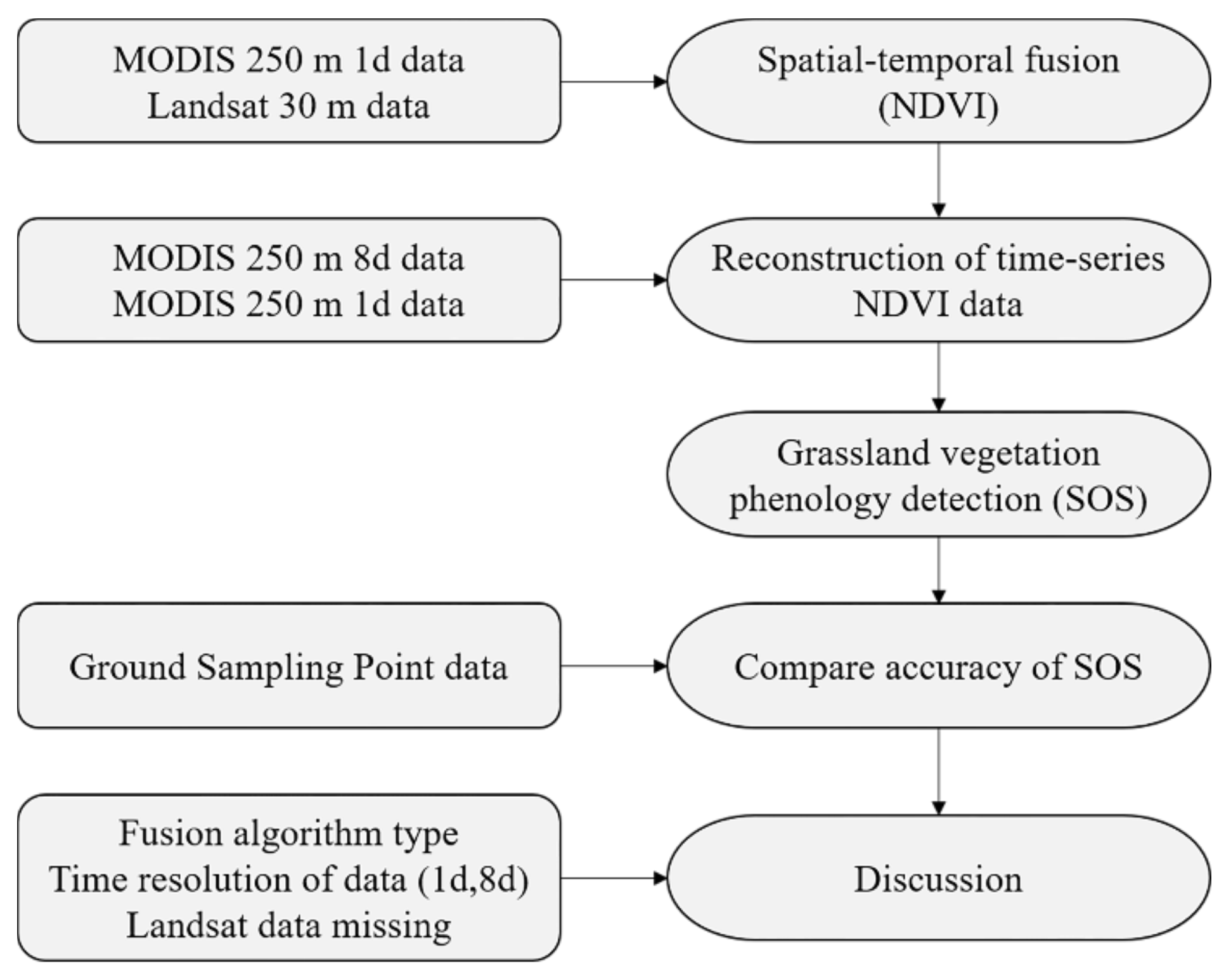
The goal of this paper is to evaluate the impact of different spatio-temporal fusion results for SOS estimation, and the related research work includes spatio-temporal fusion, time-series reconstruction, key phenology inversion, accuracy evaluation, etc. Figure 4 shows the research framework of this study.

3.1. MODIS NDVI-Landsat NDVI Spatio-Temporal Fusion

We used NDVI for fusion instead of traditional reflectance fusion. Compared with reflectance fusion (‘Blend then Index’), NDVI fusion (‘Index then Blend’) can save computing time and improve fusion accuracy [42]. As a sensitive indicator of vegetation leaf area and biomass, NDVI has been widely used in vegetation dynamic monitoring [43]. The calculation formula of NDVI is:

$$NDVI=\frac{r_{nir}-r_{red}}{r_{nir}+r_{red}}$$

(1)

where $r_{nir}$ and $r_{red}$ are the reflectance of the near-infrared and red bands, respectively.

STARFM uses a pair of Landsat-MODIS images of the base period ($T_1$) and a MODIS image of the prediction period ($T_p$) to obtain the images with 30 m resolution at the $T_p$ [27]. The formula is as follows:

$$F\left(x_{w/2},y_{w/2},t_p\right)={\displaystyle \sum }_{i=1}^w{\displaystyle \sum }_{j=1}^w{\displaystyle \sum }_{k=1}^n{w}_{ijk}\times \left(C\left(x_i,y_i,t_p\right)+F\left(x_i,y_i,t_1\right)-C\left(x_{\mathrm{i}},y_i,t_1\right)\right)$$

(2)

where $C\left(x_i,y_i\right)$ and $F\left(x_i,y_i\right)$ represent MODIS and Landsat pixels values, respectively. $w$ is the size of the sliding window, and was set as 37 × 37 (the number of Landsat pixels) by comparing the fusion accuracy of different window sizes. $\left(x_{w/2},y_{w/2},t_p\right)$ is the central pixel in the window, $w_{ijk}$ is a weight function constructed using the distance, spectral difference and temporal difference between similar image elements and target image elements to measure the influence of adjacent similar pixels to the central pixel. The formula is as follows:

$$S_{ijk}=\left|F\left(x_i,y_i,t_1\right)-C\left(x_i,y_i,t_1\right)\right|$$

(3)

$$T_{ijk}=\left|C\left(x_i,y_i,t_p\right)-C\left(x_i,y_i,t_1\right)\right|$$

(4)

$$D_{ijk}=1+\frac{\sqrt{{\left(x_{w/2}-x_i\right)}^2+{\left(y_{w/2}-y_i\right)}^2}}{750}$$

(5)

$$w_{ijk}=\frac{\left(1/\left(S_{ijk}\times T_{ijk}\times D_{ijk}\right)\right)}{{{\displaystyle \sum }}_{i=1}^w{{\displaystyle \sum }}_{j=1}^w{{\displaystyle \sum }}_{k=1}^n\left(1/\left(S_{ijk}\times T_{ijk}\times D_{ijk}\right)\right)}$$

(6)

where $S_{ijk}$ is the spectral difference used to measure the degree of heterogeneity of MODIS image elements, and $T_{ijk}$ is the temporal difference used to reflect the change in the spectra of MODIS image elements in the base period $T_1$ and the prediction period $T_p$, and $D_{ijk}$ denotes the distance between similar image elements and the central image element.

Considering the heterogeneity of MODIS pixels, USTARFM first decomposes mixed pixels of MODIS images at $T_1$ and $T_p$. Then it uses those data instead of the MODIS data in STARFM to address the problem that STARFM is difficult to search pure pixels in broken areas [35].

STDFA is based on a pair of Landsat-MODIS images of the base period ($T_1$), a final Landsat-MODIS image ($T_n$), and a MODIS image of the prediction period ($T_p$) to obtain the images with 30 m at the $T_p$ [33]. Firstly, it clustered the differential chart of Landsat images at $T_1$ and $T_n$ to capture the change information of ground objects and constitute the abundance matrix. And then, it decomposed and downscaled the MODIS images through the abundance matrix at $T_1$ ($T_n$) and $T_p$ to obtain the average value of pixel categories with the Landsat-scale at the corresponding time. Finally, assuming that the changes of the pixel values in the same type are consistent, the Landsat-scale image at $T_p$ can be expressed as:

$$r\left(c,t_p\right)=\overline{r}\left(c,t_1\right)+r\left(c,t_1\right)$$

(7)

where $r\left(c,t_p\right)$ and $\overline{r}\left(c,t_1\right)$ are the average values of the category $c$ at $T_p$ and $T_1$, respectively. $r\left(c,t_1\right)$ can be obtained from the Landsat image at the $T_1$.

We selected the Landsat images (dots with vertical lines) in Figure 2 and the MODIS image at the corresponding time to form the base period data. Next, we fused the images of the base period and the time-series MODIS images in its vicinity (where STDFA also needs to input s final Landsat image) to obtain the fusion images with Landsat-scale. Finally, the fusion images and the unused Landsat images constituted a time-series NDVI datasets with 30 m and 1 day temporal resolution in the Xilinhot for 2014–2015.

3.2. Times-Series NDVI Vegetation Index Reconstruction

The high spatio-temporal resolution NDVI datasets (30 m, 1d) were constructed by three fusion algorithms and then composited at 8d intervals by the Maximum Value Composites (MVC) algorithm [44]. Therefore, there were 6 types of fusion data which expressed as $f_{starfm}^1$, $f_{ustarfm}^1$, $f_{stdfa}^1$, $f_{starfm}^8$, $f_{ustarfm}^8$, and $f_{stdfa}^8$, where $f_n^i$ indicated the fusion data type, n indicated the fusion algorithm, and $i$ indicated the time resolution.

To reduce the noise of the time-series NDVI datasets, we fitted the datasets using the Double-Logistic (D-L) algorithm, which has good fidelity in curve fitting before the inversion of grassland SOS [45]. It can remove the pseudo-value points in the time-series curves so that the curves can better reflect the growth status of grassland vegetation. The D-L fitting function is:

$$g\left(t;a_1,\dots ,a_4\right)=\frac{1}{1+\exp \left(\frac{a_1-t}{a_2}\right)}-\frac{1}{1+\exp \left(\frac{a_3-t}{a_4}\right)}$$

(8)

where $g\left(t;a_1,\dots ,a_4\right)$ is the D-L function, $a_1$ and $a_2$ determine the inflection point of the left curve and its rate of change. $a_3$ and $a_4$ determine the inflection point of the right curve and its rate of change, respectively.

3.3. Inversion of Grassland Vegetation Phenology

This paper used the fitted NDVI datasets to acquire the SOS of grassland in 2014 and 2015 through the dynamic threshold method [46]. The dynamic threshold method defines the time when NDVI increases to a certain percentage of the current year’s NDVI amplitude as the SOS, and the time when NDVI decreases to a certain percentage as the end of the growing season (EOS). This dynamic ratio has better applicability than the absolute threshold and difference threshold [47]. The dynamic threshold method formula is:

$$NDV{I}_{lim}=\left(NDV{I}_{max}-NDV{I}_{min}\right)\times C$$

(9)

where $NDV{I}_{lim}$ is the dynamic threshold, $NDV{I}_{max}$ and $NDV{I}_{min}$ are the maximum and minimum values of NDVI in the annual growth NDVI curve, and $C$ is the coefficient that we set to 25%.

3.4. Accuracy Assessment

The correlation coefficient $R$ evaluates the correlation between the fusion data fitting NDVI vegetation index curve and the corresponding MODIS data fitting curve. The larger R indicates that the fusion data fitting curve is more similar to the MODIS fitting curve.

$$R=\frac{{{\displaystyle \sum }}_{j=1}^N\left(f_i-\overline{f}\right)\left(M_j-\overline{M}\right)}{\sqrt{{{\displaystyle \sum }}_{j=1}^N{\left(f_j-\overline{f}\right)}^2{{\displaystyle \sum }}_{j=1}^N{\left(M_j-\overline{M}\right)}^2}}$$

(10)

where $f_i$ and $M_j$ represent the value of the fusion data fitting curve and the corresponding MODIS data fitting curve at position $j$, $\overline{f}$ and $\overline{M}$ represent the mean of the fusion data fitting curve and the corresponding MODIS data fitting curve, and $N$ represents data dimensions.

The distribution characteristics of the deviations between the inversion of remote sensing images and the ground truth values, and the Root Mean Square Error (RMSE) is used to quantitatively analyze the SOS results. RMSE reflects the overall deviation between the SOS inversion from remote sensing images and the actual value of GSPs, the smaller the RMSE, the better the inversion accuracy.

$$RMSE=\sqrt{\frac{{{\displaystyle \sum }}_1^n{\left(R_i-L_i\right)}^2}{n}}$$

(11)

where $R_i$ is the SOS estimated by remote sensing method, and $L_i$ is the SOS measured at the ground sampling points.

4. Results

We compared the SOS retrieved from the fusion dataset (1d, 8d) with the SOS retrieved from the corresponding MODIS data in the study area (Figure 1), and evaluated the inversion effect of remote sensing datasets by measuring SOS on GSPs.

4.1. Grassland SOS from Remote Sensing Approaches

Although we use spatio-temporal fusion techniques to enhance the resolution of the vegetation index series, it is still difficult to accurately catch the rapid changes of vegetation over a short period using these fusion techniques. The existing spatio-temporal fusion techniques usually have an error of about 20d when performing vegetation SOS extraction [48]. Taking this issue into account, we fitted the data using the D-L algorithm. Then MVC method was used to highlight the characteristics of vegetation changes as much as possible in local time. Based on this, we compared the overall inversion results using 8d composite data with MODIS data.

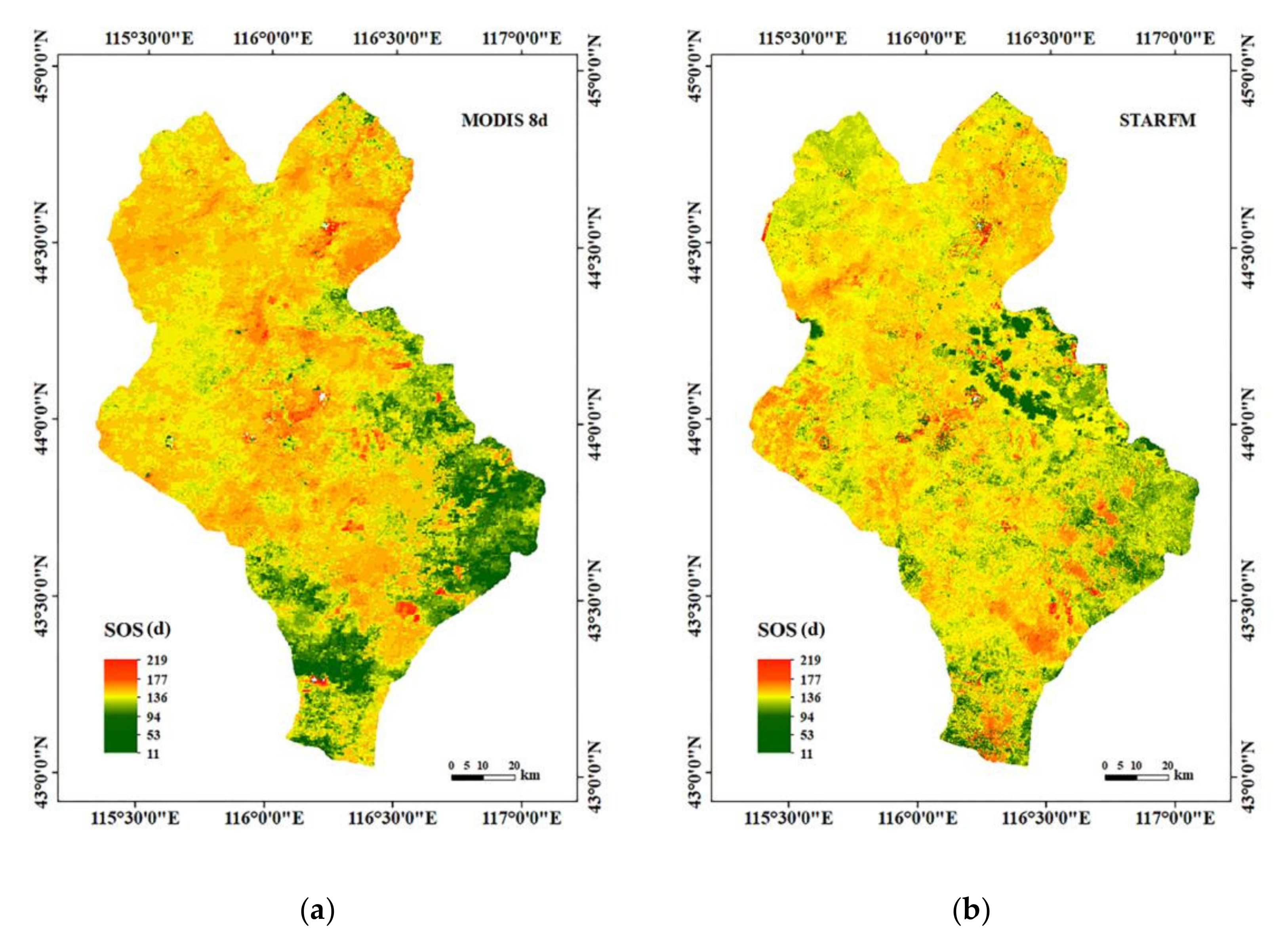
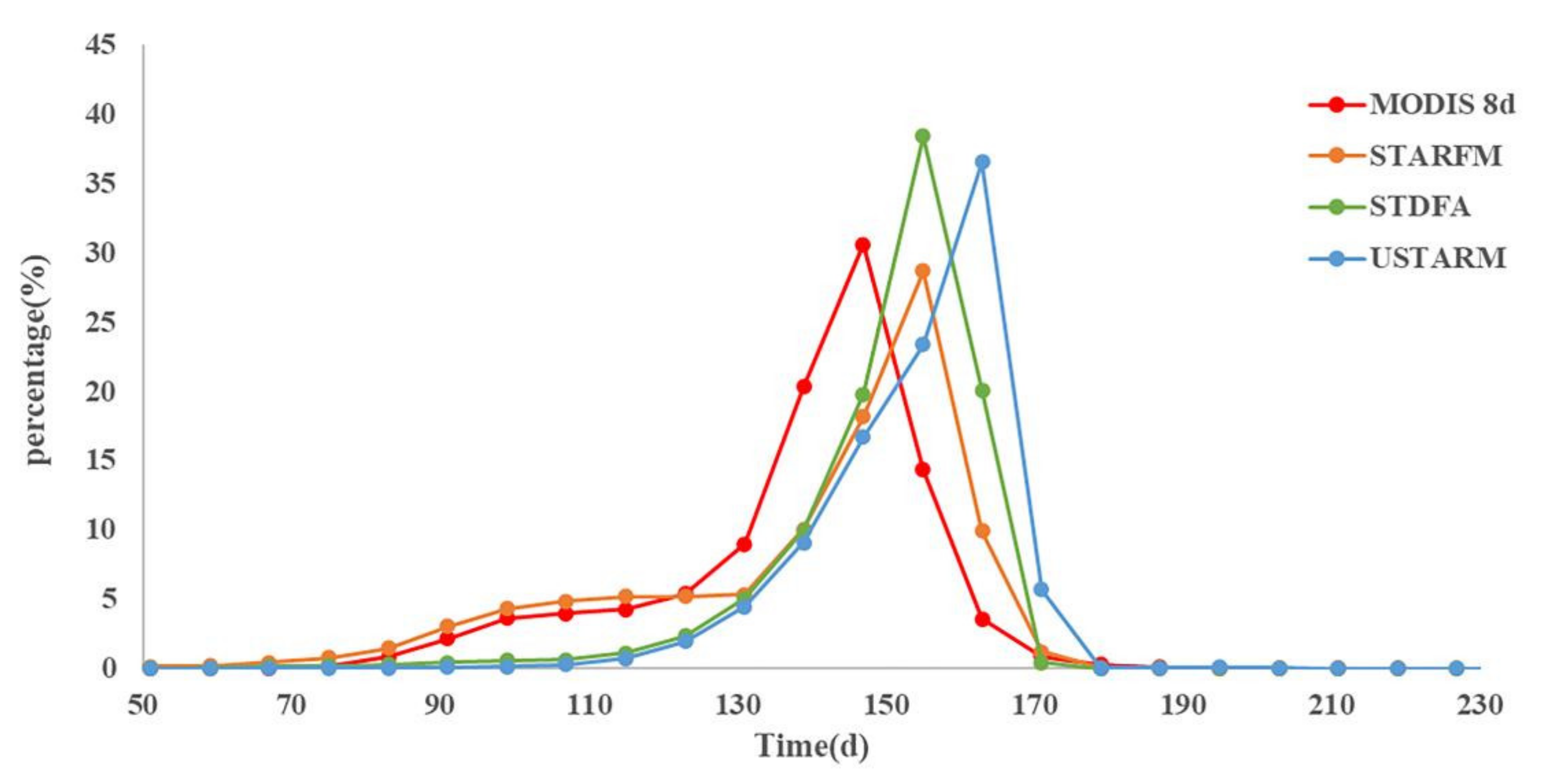
The overall trend of the SOS of inversion $f_{starfm}^8$ was consistent with the result of $M^8$, whereby Xilinhot East and Southwest are the first to return to green, while North is relatively late (Figure 5). In early April, part of the study areas began to re-green in the results of $f_{starfm}^8$ and $M^8$ (Figure 6). The SOS inversion of the four types of data lasted from mid-April to about mid-June. Compared with the MODIS inversion results, the SOS inversions of the three fusion data were delayed. Through the qualitative analysis of the inversion trend of the overall SOS in the study area, the results of the SOS using STARFM fusion data for Xilinhot may have a better inversion effect.

4.2. SOS Inversion Accuracy Analysis with Ground Sampling Data

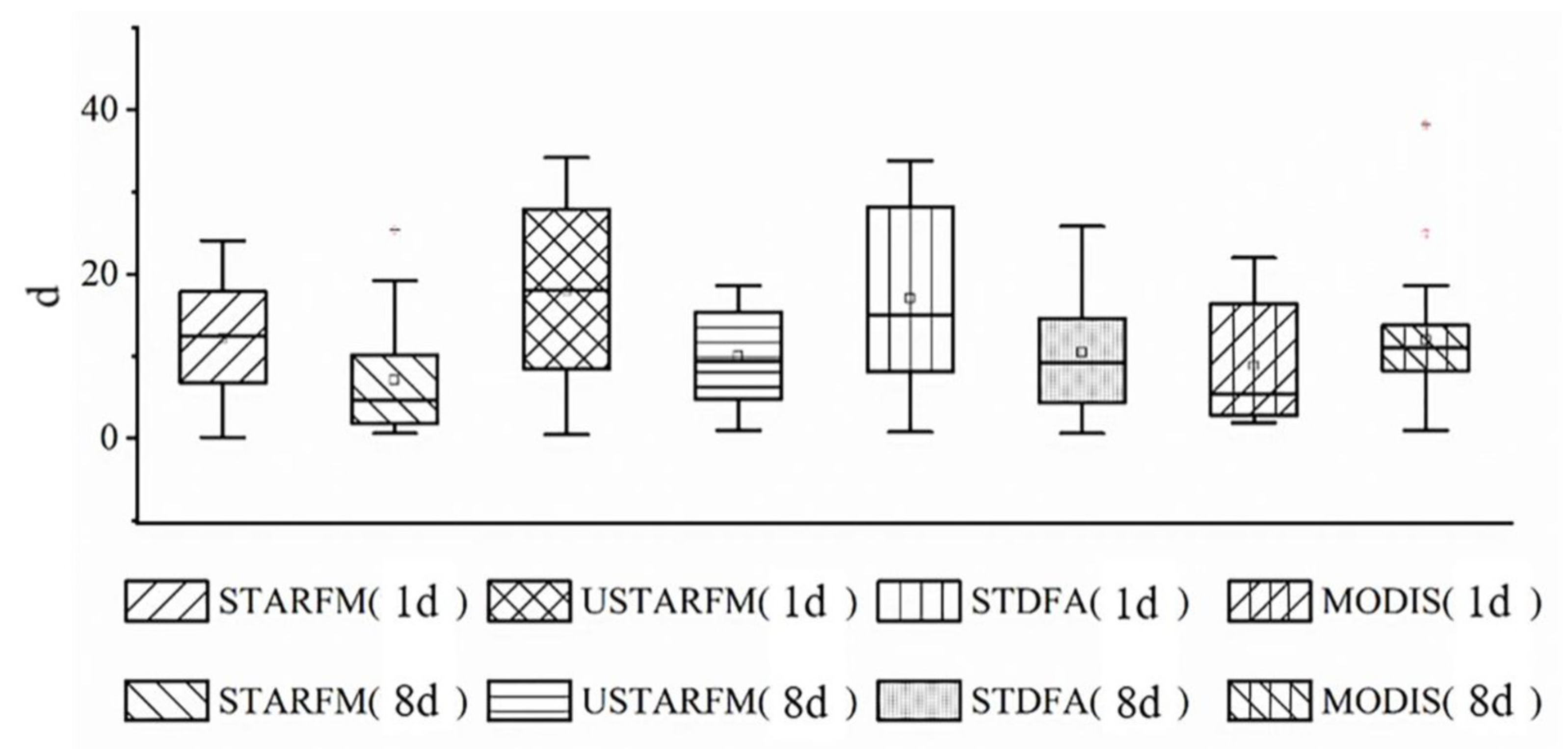
Figure 7 and

Table 1. RMSE between the SOS inversion and ground measured SOS at GSPs.

Datasets	${\mathit{f}}_{\mathit{s}\mathit{t}\mathit{a}\mathit{r}\mathit{f}\mathit{m}}^1$	${\mathit{f}}_{\mathit{s}\mathit{t}\mathit{a}\mathit{r}\mathit{f}\mathit{m}}^8$	${\mathit{f}}_{\mathit{u}\mathit{s}\mathit{t}\mathit{a}\mathit{r}\mathit{f}\mathit{m}}^1$	${\mathit{f}}_{\mathit{u}\mathit{s}\mathit{t}\mathit{a}\mathit{r}\mathit{f}\mathit{m}}^8$	${\mathit{f}}_{\mathit{s}\mathit{t}\mathit{d}\mathit{f}\mathit{a}}^1$	${\mathit{f}}_{\mathit{s}\mathit{t}\mathit{d}\mathit{f}\mathit{a}}^8$	${\mathit{M}}^1$	${\mathit{M}}^8$
RMSE	13.7d	9.7d	20.6d	11.0d	20.2d	12.6d	11.3d	14.3d

, the SOS retrieved from 8d dataset was generally closer to the ground measured value, and the deviation distribution was more concentrated than the daily fusion data. The most concentrated data of the deviation distribution was $M^8$, then $f_{starfm}^8$ and $f_{stdfa}^8$. The average absolute value of the deviation between the $f_{starfm}^8$ result and the measured value was the smallest at 8.7d, and the absolute value of the deviation of 50% of the sampling points was in the range of 3d–12.2d. Additionally, the absolute value of the deviation of the inversion using $f_{ustarfm}^1$ was the largest at 18d, and the absolute value of the deviation of 50% of the sampling points was concentrated in 8.5d–27.9d. The RMSE of $M^1$ and $M^8$ data were 11.3d and 14.3d respectively, which shown that remote sensing identification of vegetation SOS in Xilinhot based on MODIS data is feasible [48]. The RMSE of $f_{starfm}^8$ data inversion was the smallest, which was 9.7d, and the maximum RMES was 20.6d of the $f_{ustarfm}^1$ (Table 1). Among the fusion data, the inversion accuracy of the 8d data in the SOS was better than that of the daily fusion data and the $M^8$ data. The inversion accuracy of the $f_{starfm}^8$ and $f_{ustarfm}^8$ were higher than the $M^1$. However, the accuracy of the daily fusion data inversion of the three algorithms was lower than that of the $M^1$, while the accuracy of the $f_{starfm}^1$ was better than the $M^8$.

5. Discussion

5.1. Analysis of SOS Inversion Results for Different Algorithms

The USTARFM algorithm is an improvement on the STARFM algorithm, and it mainly eliminates image spots in STARFM fusion data and increases the probability of finding pure pixels in the window to improve the accuracy. Therefore, the fusion accuracy of STDFA and USTARFM algorithms was better than that of the STARFM algorithm in heterogeneous regions. However, we compared the overall inversion results using 8d composite data with MODIS data. By analyzing the spatial distribution of the SOS in the study area obtained by the inversion of different datasets, it was found that the inversion effect of STARFM data is relatively better (Figure 8), which may be related to the fact that the ground object type of the study area is mainly grassland, and most of them belong to the homogeneous area. Therefore, the fusion accuracy of the STARFM algorithm is relatively higher than the other two algorithms. In order to further analyze the inversion results of each fusion data, we compared the six fusion datasets with the measured SOS for quantitative analysis. The results shown that the NDVI datasets constructed by spatio-temporal fusion technology had better performance in the inversion of grassland SOS than MODIS data. Among these fusion algorithms, the STARFM was the best for the SOS inversion (Figure 8). The MODIS daily data are affected by uncontrollable factors such as climate, and the images have a lot of noise. Therefore, the fitting effect of D-L function on daily fusion data is poor, which will affect the accuracy of SOS. In addition, the results of daily fusion data cannot well capture the rapid changes of vegetation during the SOS, which is also one of the reasons for its low accuracy in SOS inversion. Multi-days composite data can offset the shortage of daily fusion data slightly, which improves the accuracy of SOS inversion.

5.2. Correlation Analysis of Different NDVI Time Series

Long time-series NDVI data can monitor the growth and change process of vegetation and are the basis for subsequent key phenology detection. Using fusion data and a curve fit of MODIS data, we then evaluated the effect of time-series NDVI fusion data that can reflect grassland vegetation status.

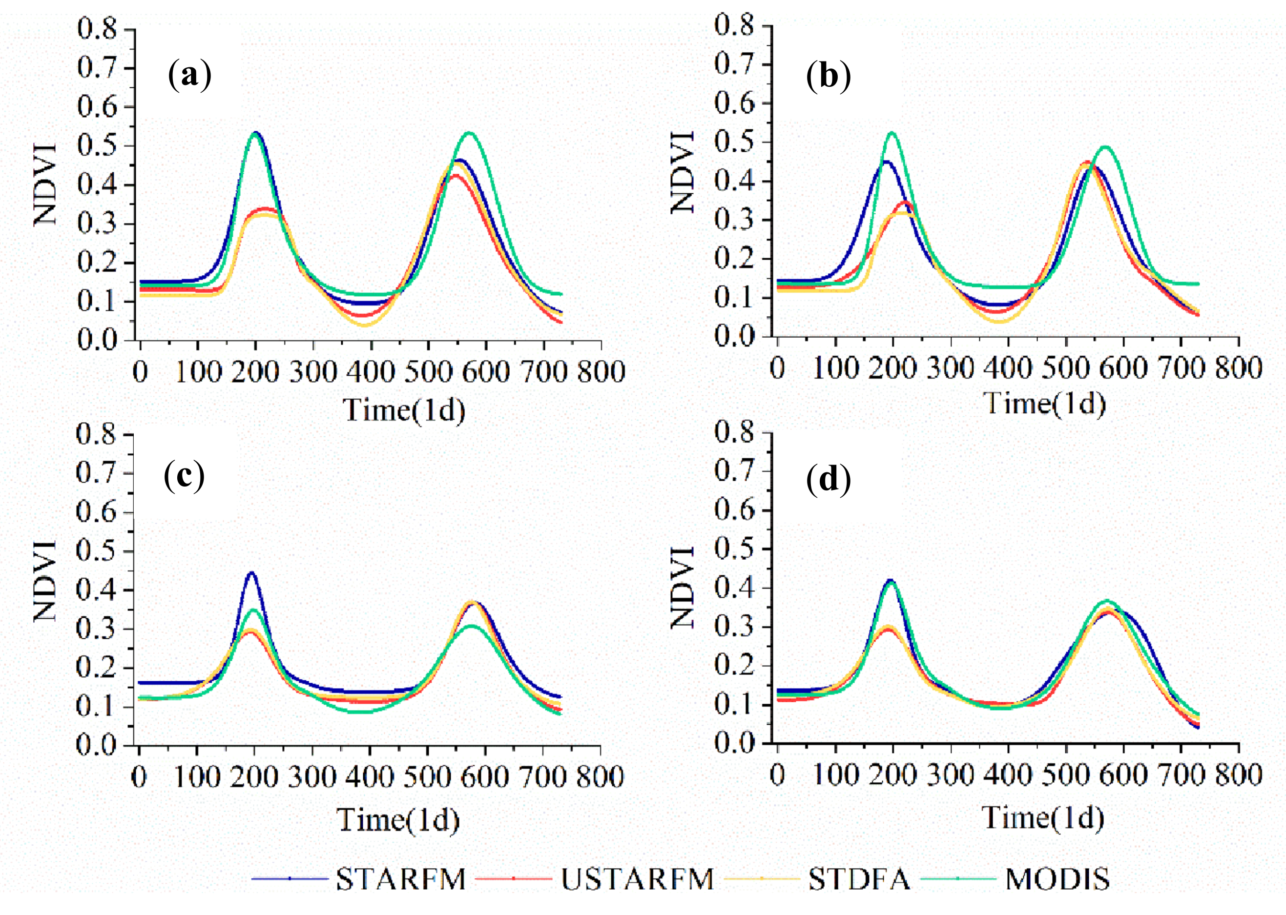
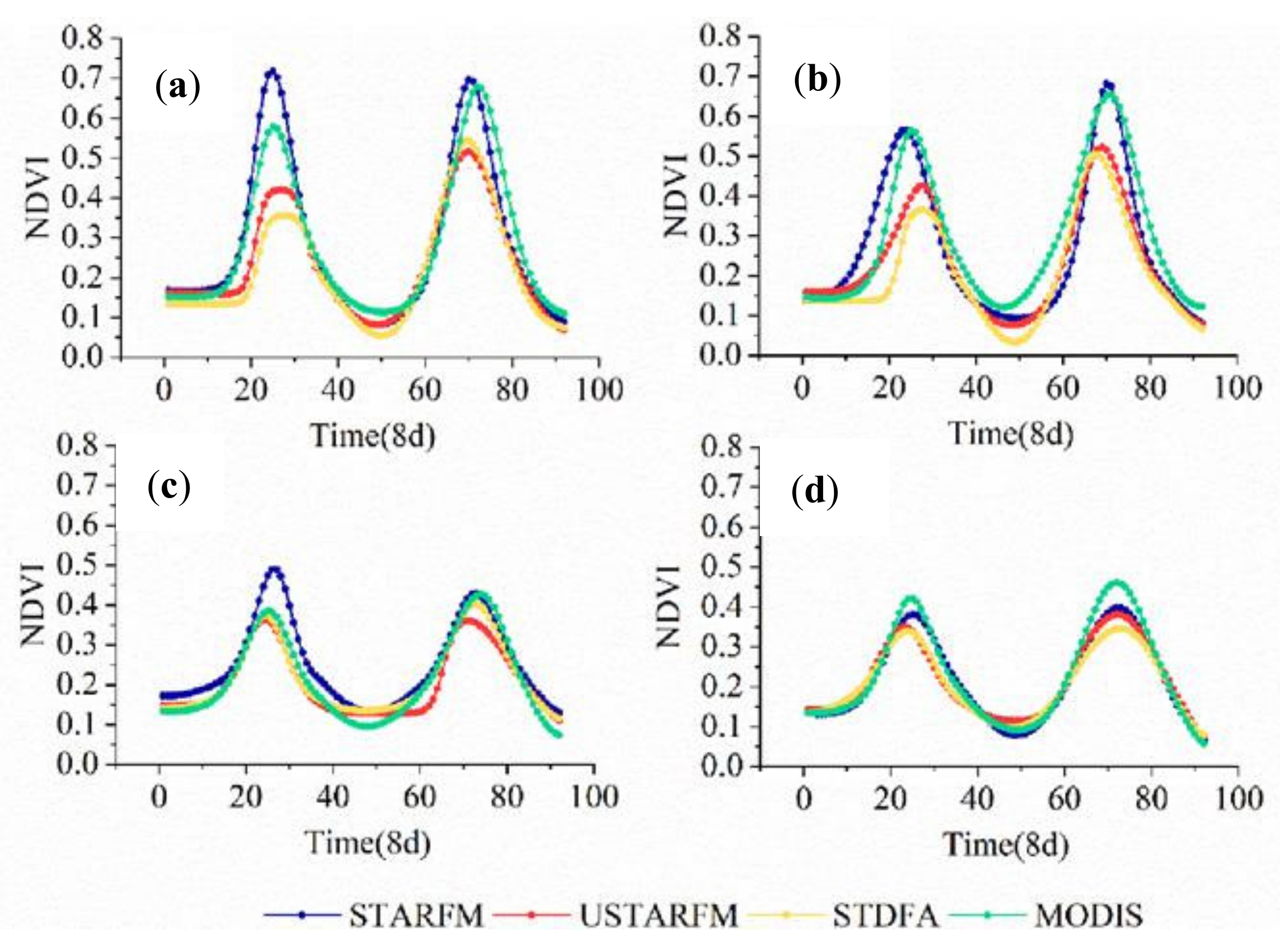
As shown in Figure 9 and Figure 10 and

Table 2. The R between the fitting curve of each fusion data and the corresponding MODIS.

GSP	${\mathit{f}}_{\mathit{s}\mathit{t}\mathit{a}\mathit{r}\mathit{f}\mathit{m}}^1$	${\mathit{f}}_{\mathit{s}\mathit{t}\mathit{a}\mathit{r}\mathit{f}\mathit{m}}^8$	${\mathit{f}}_{\mathit{u}\mathit{s}\mathit{t}\mathit{a}\mathit{r}\mathit{f}\mathit{m}}^1$	${\mathit{f}}_{\mathit{u}\mathit{s}\mathit{t}\mathit{a}\mathit{r}\mathit{f}\mathit{m}}^8$	${\mathit{f}}_{\mathit{s}\mathit{t}\mathit{d}\mathit{f}\mathit{a}}^1$	${\mathit{f}}_{\mathit{s}\mathit{t}\mathit{d}\mathit{f}\mathit{a}}^8$
a *	0.963	0.964	0.902	0.950	0.901	0.916
b *	0.915	0.917	0.846	0.941	0.846	0.931
c *	0.971	0.977	0.952	0.969	0.954	0.961
d *	0.981	0.993	0.995	0.983	0.968	0.982

* Sampling points a and b are from strip No. 124029 2014, while sampling points c and d are from strip No. 124030 2015.

, the six types of fitting curves of time-series NDVI data were consistent with the corresponding MODIS data fitting curves, and the R were all above 0.8, which could better describe the grassland vegetation status. Due to a large amount of noise in daily data, D-L fitting method cannot smooth the noise well, and the smoothness of the fitting curve was low, and the overall effect of the reconstructed curve ($\overline{R}$= 0.933) was lower than that of 8d data ($\overline{R}$= 0.957). In the NDVI data sets of the three algorithms, STARFM 8d data reconstruction curve ($\overline{R}$= 0.963) and daily data reconstruction curve ($\overline{R}$= 0.958) had better ability to describe grassland vegetation growth than the other two algorithms, and were closer to the vegetation growth curve fitted by MODIS data. The R between the fitting curves of fusion data and the corresponding MODIS data fitting curves of sampling points a and b was lower than those of sampling points c and d. In the first half of 2014, the fitting curves of the fusion data and the MODIS data for a and b sets of sampling points were quite different (Figure 9 and Figure 10). Due to the absence of Landsat base period data in the vicinity of the SOS at the two sampling sites in 2014, we can wonder whether the lack of base period data in the vicinity of the SOS will reduce the inversion accuracy of the fusion data.

5.3. The Impact of Missing Landsat Data during SOS

During data fusion, this paper used multi-period Landsat images and continuous MODIS images to construct continuous NDVI data, and then inverted the vegetation SOS. However, due to the influence of weather (cloud contamination), the acquisition interval of Landsat images was too long and the images were incomplete during the SOS (Figure 11), which resulted in possible failure to capture the changes in vegetation growth and reduced the constraints of fusion, making the poor fusion effect in one year.

For the two sampling points (a and b) in 2014, the overall NDVI time series curves reconstructed by using each fusion data showed some deviation from the reconstructed curves of MODIS data, and the RMSE were lower than those of c and d (Figure 9 and Figure 10, Table 2). To find the reason, we analyzed the original data from both years and found that the Landsat image in the vegetation SOS in 2014 was missing an image, which may lead to a poor fusion effect in this year, reducing the accuracy of the SOS inversion. To explore whether the absence of Landsat images during SOS will reduce the inversion accuracy, as well as to examine the differences in the predictive power of different fusion models for this sudden perturbation information. Therefore, based on different spatio-temporal fusion algorithms, this paper removed a Landsat image in the vicinity of the SOS in 2015 and then compared the accuracy of the two SOS inversion results.

Firstly, we removed the Landsat data at the time point of the yellow rectangular box in Figure 2 (NO. 124029, the green dot in 2015). Then used continuous MODIS data to fuse with it to build high spatio-temporal resolution NDVI data. Next, we obtained SOS inversion by using NDVI data and its MVC 8d data, and compared them with the SOS inversion by using the measured data and the full data.

When Landsat data was missing in SOS, the inversion accuracy of the fusion data would decrease by varying degrees (Figure 12,

Table 3. RMSE between the SOS inversion and ground measured SOS.

Data Source	STARFM		USTARFM		STDFA
Processing Method	Full *	Missing	Full	Missing	Full	Missing
Daily	14.8d	15.2d	23.6d	35.5d	23.6d	43.1d
8d data	9.5d	14.5d	12.7d	29.7d	15.6d	28.2d

* The base period data is not removed.

). The SOS inversion using the data fused by STARFM or STDFA was delayed by varying degrees; meanwhile, it was just the opposite with the SOS inversion using the data fused by USTARFM, which started to return to green early. When the Landsat data in SOS was incomplete, the STARFM was the least affected, $\overline{RMSE}$ increased by 2.7d; the STDFA was the most affected, $\overline{RMSE}$ increased by 16d (Table 3).

In spatio-temporal data fusion, when the Landsat data in the vicinity of the SOS is missing, the quality of the fusion image in the vicinity is reduced, resulting in a decrease in the inversion accuracy. The three algorithms of STARFM, USTARFM, and STDFA have poor predictive capabilities for this sudden disturbance information. However, the loss of Landsat image caused by the weather is unavoidable. At this time, we can choose the STARFM model to minimize the loss of accuracy caused by the lack of images.

6. Conclusions

This paper fused Landsat and MODIS data from 2014–2015 using three fusion algorithms (STARFM, USTARFM, and STDFA) to obtain the NDVI dataset. It was fitted using the D-L function, which could remove the pseudo-value points in the time-series curves, meaning that the NDVI curves can better reflect the growth status of grassland vegetation. Then, through the MVC method, we tried to ensure that the characteristics of vegetation changes can be highlighted to the maximum extent in local time. Finally, we compared the SOS obtained from various fused data with the ground truth to quantitatively analyze the effect of different algorithms. Based on this, the effects of different factors on SOS accuracy were analyzed and discussed.

Our study demonstrated that the SOS inversion of 8d data from the fusion of the three algorithms was better than that of daily data, and the SOS inversion accuracy of $f_{starfm}^8$ data was the best, which is closer to the ground measured data. Compared with USTARFM and STDFA, STARFM is more suitable for grassland vegetation phenology monitoring. Grassland vegetation grows and changes rapidly, especially in the SOS. When the SOS of vegetation lacks a Landsat image, it was difficult to capture the changes of vegetation, resulting in a decrease in the quality of the fusion data that year, thus affecting the SOS inversion accuracy. And the three models were affected differently by missing data, and the fusion data of the STARFM algorithm was least affected. This study exemplifies the potential of spatio-temporal fusion methods in improving the SOS inversion accuracy of grassland vegetation, and laid the foundation for future applications in spatio-temporal fusion techniques in grassland vegetation monitoring.

References

1. Altesor, A.; Oesterheld, M.; Leoni, E.; Lezama, F.; Rodriguez, C. Effect of grazing on community structure and productivity of a Uruguayan grassland. Plant Ecol. 2005, 179, 83–91. [Google Scholar] [CrossRef]
2. Lu, P.L.; Yu, Q.; He, Q.T. Responses of plant phenology to climatic change. Acta Ecol. Sin. 2006, 26, 929. [Google Scholar] [CrossRef]
3. Cleland, E.E.; Chiariello, N.R.; Loarie, S.R.; Mooney, H.A.; Field, C.B. Diverse responses of phenology to global changes in a grassland ecosystem. Proc. Natl. Acad. Sci. USA 2006, 103, 13740–13744. [Google Scholar] [CrossRef] [PubMed] [Green Version]
4. Yoshie, F. Effects of growth temperature and winter duration on leaf phenology of a spring ephemeral (Gagea lutea) and a summergreen forb (Maianthemum dilatatum). J. Plant Res. 2008, 121, 483–492. [Google Scholar] [CrossRef] [PubMed]
5. Hou, J.; Du, L.T.; Liu, K.; Hu, Y.; Zhu, Y.G. Characteristics of vegetation activity and its responses to climate change in desert/grassland biome transition zones in the last 30years based on GIMMS3g. Theor. Appl. Climatol. 2019, 136, 915–928. [Google Scholar] [CrossRef]
6. Wang, G.C.; Huang, Y.; Wei, Y.R.; Zhang, W.; Li, T.T.; Zhang, Q. Inner Mongolian grassland plant phenological changes and their climatic drivers. Sci. Total Environ. 2019, 683, 1–8. [Google Scholar] [CrossRef] [PubMed]
7. Lee, R.; Yu, F.; Price, K.P.; Ellis, J.; Shi, P. Evaluating vegetation phenological patterns in Inner Mongolia using NDVI time-series analysis. Int. J. Remote Sens. 2002, 23, 2505–2512. [Google Scholar] [CrossRef]
8. Myneni, R.B.; Keeling, C.D.; Tucker, C.J.; Asrar, G.; Nemani, R.R. Increased plant growth in the northern high latitudes from 1981 to 1991. Nature 1997, 386, 698–702. [Google Scholar] [CrossRef]
9. Garonna, I.; de Jong, R.; Schaepman, M.E. Variability and evolution of global land surface phenology over the past three decades (1982–2012). Glob. Change Biol. 2016, 22, 1456–1468. [Google Scholar] [CrossRef]
10. Gu, S.; Tang, Y.H.; Cui, X.Y.; Kato, T.; Du, M.Y.; Li, Y.N.; Zhao, X.Q. Energy exchange between the atmosphere and a meadow ecosystem on the Qinghai-Tibetan Plateau. Agric. For. Meteorol. 2005, 129, 175–185. [Google Scholar] [CrossRef]
11. Schwartz, M.D.; Ahas, R.; Aasa, A. Onset of spring starting earlier across the Northern Hemisphere. Glob. Change Biol. 2006, 12, 343–351. [Google Scholar] [CrossRef]
12. Menzel, A.; Sparks, T.H.; Estrella, N.; Roy, D.B. Altered geographic and temporal variability in phenology in response to climate change. Glob. Ecol. Biogeogr. 2006, 15, 498–504. [Google Scholar] [CrossRef]
13. Reed, B.C.; Brown, J.F. Trend analysis of time-series phenology derived from satellite data. In Proceedings of the 3rd International Workshop on the Analysis of Multi-Temporal Remote Sensing Images, Biloxi, MS, USA, 16–18 May 2005; pp. 166–168. [Google Scholar]
14. White, M.A.; Thornton, P.E.; Running, S.W. A continental phenology model for monitoring vegetation responses to interannual climatic variability. Glob. Biogeochem. Cycle 1997, 11, 217–234. [Google Scholar] [CrossRef]
15. Stockli, R.; Vidale, P.L. European plant phenology and climate as seen in a 20-year AVHRR land-surface parameter dataset. Int. J. Remote Sens. 2004, 25, 3303–3330. [Google Scholar] [CrossRef]
16. Zhou, J.H.; Cai, W.T.; Qin, Y.; Lai, L.M.; Guan, T.Y.; Zhang, X.L.; Jiang, L.H.; Du, H.; Yang, D.W.; Cong, Z.T.; et al. Alpine vegetation phenology dynamic over 16years and its covariation with climate in a semi-arid region of China. Sci. Total Environ. 2016, 572, 119–128. [Google Scholar] [CrossRef]
17. Zhang, Q.; Kong, D.D.; Shi, P.J.; Singh, V.P.; Sun, P. Vegetation phenology on the Qinghai-Tibetan Plateau and its response to climate change (1982–2013). Agric. For. Meteorol. 2018, 248, 408–417. [Google Scholar] [CrossRef]
18. Shen, X.J.; Liu, B.H.; Xue, Z.S.; Jiang, M.; Lu, X.G.; Zhang, Q. Spatiotemporal variation in vegetation spring phenology and its response to climate change in freshwater marshes of Northeast China. Sci. Total Environ. 2019, 666, 1169–1177. [Google Scholar] [CrossRef]
19. Reed, B.C.; Brown, J.F.; Vanderzee, D.; Loveland, T.R.; Merchant, J.W.; Ohlen, D.O. Measuring phenological variability from satellite imagery. J. Veg. Sci. 1994, 5, 703–714. [Google Scholar] [CrossRef]
20. Jeong, S.J.; Ho, C.H.; Gim, H.J.; Brown, M.E. Phenology shifts at start vs. end of growing season in temperate vegetation over the Northern Hemisphere for the period 1982–2008. Glob. Change Biol. 2011, 17, 2385–2399. [Google Scholar] [CrossRef]
21. Hmimina, G.; Dufrene, E.; Pontailler, J.Y.; Delpierre, N.; Aubinet, M.; Caquet, B.; de Grandcourt, A.; Burban, B.; Flechard, C.; Granier, A.; et al. Evaluation of the potential of MODIS satellite data to predict vegetation phenology in different biomes: An investigation using ground-based NDVI measurements. Remote Sens. Environ. 2013, 132, 145–158. [Google Scholar] [CrossRef]
22. Zhou, Q.; Rover, J.; Brown, J.; Worstell, B.; Howard, D.; Wu, Z.T.; Gallant, A.L.; Rundquist, B.; Burke, M. Monitoring Landscape Dynamics in Central US Grasslands with Harmonized Landsat-8 and Sentinel-2 Time Series Data. Remote Sens. 2019, 11, 328. [Google Scholar] [CrossRef] [Green Version]
23. Brown, J.F.; Howard, D.; Wylie, B.; Frieze, A.; Ji, L.; Gacke, C. Application-Ready Expedited MODIS Data for Operational Land Surface Monitoring of Vegetation Condition. Remote Sens. 2015, 7, 16226–16240. [Google Scholar] [CrossRef] [Green Version]
24. Kovalskyy, V.; Roy, D.P.; Zhang, X.; Ju, J.C. The suitability of multi-temporal web-enabled Landsat data NDVI for phenological monitoring—A comparison with flux tower and MODIS NDVI. Remote Sens. Lett. 2012, 3, 325–334. [Google Scholar] [CrossRef]
25. Snyder, K.A.; Huntington, J.L.; Wehan, B.L.; Morton, C.G.; Stringham, T.K. Comparison of Landsat and Land-Based Phenology Camera Normalized Difference Vegetation Index (NDVI) for Dominant Plant Communities in the Great Basin. Sensors 2019, 19, 1139. [Google Scholar] [CrossRef] [Green Version]
26. Yan, L.; Roy, D.P. Large-Area Gap Filling of Landsat Reflectance Time Series by Spectral-Angle-Mapper Based Spatio-Temporal Similarity (SAMSTS). Remote Sens. 2018, 10, 609. [Google Scholar] [CrossRef] [Green Version]
27. Gao, F.; Masek, J.; Schwaller, M.; Hall, F. On the blending of the Landsat and MODIS surface reflectance: Predicting daily Landsat surface reflectance. IEEE Trans. Geosci. Remote Sens. 2006, 44, 2207–2218. [Google Scholar] [CrossRef]
28. Zhu, X.L.; Cai, F.Y.; Tian, J.Q.; Williams, T.K.A. Spatiotemporal Fusion of Multisource Remote Sensing Data: Literature Survey, Taxonomy, Principles, Applications, and Future Directions. Remote Sens. 2018, 10, 527. [Google Scholar] [CrossRef] [Green Version]
29. Zhukov, B.; Oertel, D.; Lanzl, F.; Reinhackel, G. Unmixing-based multisensor multiresolution image fusion. IEEE Trans. Geosci. Remote Sens. 1999, 37, 1212–1226. [Google Scholar] [CrossRef]
30. Hilker, T.; Wulder, M.A.; Coops, N.C.; Linke, J.; McDermid, G.; Masek, J.G.; Gao, F.; White, J.C. A new data fusion model for high spatial- and temporal-resolution mapping of forest disturbance based on Landsat and MODIS. Remote Sens. Environ. 2009, 113, 1613–1627. [Google Scholar] [CrossRef]
31. Zhu, X.L.; Chen, J.; Gao, F.; Chen, X.H.; Masek, J.G. An enhanced spatial and temporal adaptive reflectance fusion model for complex heterogeneous regions. Remote Sens. Environ. 2010, 114, 2610–2623. [Google Scholar] [CrossRef]
32. Huang, B.; Song, H.H. Spatiotemporal Reflectance Fusion via Sparse Representation. IEEE Trans. Geosci. Remote Sens. 2012, 50, 3707–3716. [Google Scholar] [CrossRef]
33. Wu, M.Q.; Niu, Z.; Wang, C.Y.; Wu, C.Y.; Wang, L. Use of MODIS and Landsat time series data to generate high-resolution temporal synthetic Landsat data using a spatial and temporal reflectance fusion model. J. Appl. Remote Sens. 2012, 6, 063507. [Google Scholar] [CrossRef]
34. Song, H.H.; Huang, B. Spatiotemporal Satellite Image Fusion Through One-Pair Image Learning. IEEE Trans. Geosci. Remote Sens. 2013, 51, 1883–1896. [Google Scholar] [CrossRef]
35. Xie, D.F.; Zhang, J.S.; Zhu, X.F.; Pan, Y.Z.; Liu, H.L.; Yuan, Z.M.Q.; Yun, Y. An Improved STARFM with Help of an Unmixing-Based Method to Generate High Spatial and Temporal Resolution Remote Sensing Data in Complex Heterogeneous Regions. Sensors 2016, 16, 207. [Google Scholar] [CrossRef] [PubMed] [Green Version]
36. Song, H.H.; Liu, Q.S.; Wang, G.J.; Hang, R.L.; Huang, B. Spatiotemporal Satellite Image Fusion Using Deep Convolutional Neural Networks. IEEE J. Sel. Top. Appl. Earth Observ. Remote Sens. 2018, 11, 821–829. [Google Scholar] [CrossRef]
37. Liu, W.J.; Zeng, Y.N.; Li, S.N.; Pi, X.Y.; Huang, W. An Improved Spatiotemporal Fusion Approach Based on Multiple Endmember Spectral Mixture Analysis. Sensors 2019, 19, 2443. [Google Scholar] [CrossRef] [Green Version]
38. Walker, J.J.; de Beurs, K.M.; Wynne, R.H. Dryland vegetation phenology across an elevation gradient in Arizona, USA, investigated with fused MODIS and Landsat data. Remote Sens. Environ. 2014, 144, 85–97. [Google Scholar] [CrossRef]
39. Gao, F.; Anderson, M.C.; Zhang, X.Y.; Yang, Z.W.; Alfieri, J.G.; Kustas, W.P.; Mueller, R.; Johnson, D.M.; Prueger, J.H. Toward mapping crop progress at field scales through fusion of Landsat and MODIS imagery. Remote Sens. Environ. 2017, 188, 9–25. [Google Scholar] [CrossRef] [Green Version]
40. Onojeghuo, A.O.; Blackburn, G.A.; Wang, Q.M.; Atkinson, P.M.; Kindred, D.; Miao, Y.X. Rice crop phenology mapping at high spatial and temporal resolution using downscaled MODIS time-series. GISci. Remote Sens. 2018, 55, 659–677. [Google Scholar] [CrossRef] [Green Version]
41. Lyu, X.; Li, X.B.; Dang, D.L.; Dou, H.S.; Xuan, X.J.; Liu, S.Y.; Li, M.Y.; Gong, J.R. A new method for grassland degradation monitoring by vegetation species composition using hyperspectral remote sensing. Ecol. Indic. 2020, 114, 106310. [Google Scholar] [CrossRef]
42. Jarihani, A.A.; McVicar, T.R.; Van Niel, T.G.; Emelyanova, I.V.; Callow, J.N.; Johansen, K. Blending Landsat and MODIS Data to Generate Multispectral Indices: A Comparison of “Index-then-Blend” and “Blend-then-Index” Approaches. Remote Sens. 2014, 6, 9213–9238. [Google Scholar] [CrossRef] [Green Version]
43. Di Bella, C.; Faivre, R.; Ruget, F.; Seguin, B.; Guerif, M.; Combal, B.; Weiss, A.; Rebella, C. Remote sensing capabilities to estimate pasture production in France. Int. J. Remote Sens. 2004, 25, 5359–5372. [Google Scholar] [CrossRef]
44. Holben, B.N. Characteristics of maximum-value composite images from temporal AVHRR data. Int. J. Remote Sens. 1986, 7, 1417–1434. [Google Scholar] [CrossRef]
45. Guo, J.; Yang, X.C.; Niu, J.M.; Jin, Y.X.; Xu, B.; Shen, G.; Zhang, W.B.; Zhao, F.; Zhang, Y.J. Remote sensing monitoring of green-up dates in the Xilingol grasslands of northern China and their correlations with meteorological factors. Int. J. Remote Sens. 2019, 40, 2190–2211. [Google Scholar] [CrossRef]
46. Jonsson, P.; Eklundh, L. Seasonality extraction by function fitting to time-series of satellite sensor data. IEEE Trans. Geosci. Remote Sens. 2002, 40, 1824–1832. [Google Scholar] [CrossRef]
47. Jonsson, P.; Eklundh, L. TIMESAT—A program for analyzing time-series of satellite sensor data. Comput. Geosci. 2004, 30, 833–845. [Google Scholar] [CrossRef] [Green Version]
48. Xin, Q.C.; Broich, M.; Zhu, P.; Gong, P. Modeling grassland spring onset across the Western United States using climate variables and MODIS-derived phenology metrics. Remote Sens. Environ. 2015, 161, 63–77. [Google Scholar] [CrossRef]
Figure 1. Grass classification map and ground sampling point distribution map in the study area.
Remotesensing 14 02542 g001
Figure 2. The date of Landsat image acquisition. Where the dots on the horizontal axis of DOY (Day of Year) are the transit time of Landsat, 124029 and 124030 are the Landsat swath ID, and the red and green dots represent Landsat images in 2014 and 2015, respectively.
Remotesensing 14 02542 g002
Figure 3. Sample box with GSPs in ground measurement in mid-April 2015.
Remotesensing 14 02542 g003
Figure 4. Flowchart of exploring the effectiveness of different fusion algorithms in SOS inversion.
Remotesensing 14 02542 g004
Figure 5. Spatial distribution of SOS in Xilinhot inverted by using different datasets in 2015. (a) SOS inversion with MODIS 8d data;(bd) SOS inversion with STARFM, STDFA, USTARFM 8d data.
Remotesensing 14 02542 g005aRemotesensing 14 02542 g005b
Figure 6. The trend of SOS inversion with four types of data in 2015.
Remotesensing 14 02542 g006
Figure 7. The deviation distribution of the SOS inversion at GSPs. (a) Stands for ‘the data’ is daily data. (b) Stands for ‘the data’ is MVC 8d data.
Remotesensing 14 02542 g007
Figure 8. Box plot of AD (average deviation) distribution between the SOS inversion and ground measured SOS.
Remotesensing 14 02542 g008
Figure 9. Daily data fitting curve (x-axis scale interval is 1d, from 2014 to 2015). Sampling points (a,b) are from strip No. 124029 2014, while sampling points (c,d) are from strip No. 124030 2015.
Remotesensing 14 02542 g009
Figure 10. MVC 8d data fitting curve (x-axis scale interval is 8d, from 2014 to 2015). Sampling points (a,b) are from strip No. 124029 2014, while sampling points (c,d) are from strip No. 124030 2015.
Remotesensing 14 02542 g010
Figure 11. NDVI curve of vegetation for one year.
Remotesensing 14 02542 g011
Figure 12. The deviation distribution of the SOS inversion using the data and ground measured SOS in 2015 (NO. 124029). M in STARFM (M) means the Landsat data is missing.
Remotesensing 14 02542 g012